A Bearing Fault Diagnosis Method Using Multi-Branch Deep Neural Network

Abstract

Feature extraction from a signal is the most important step in signal-based fault diagnosis. Deep learning or deep neural network (DNN) is an effective method to extract features from signals. In this paper, a novel vibration signal-based bearing fault diagnosis method using DNN is proposed. First, the measured vibration signals are transformed into a new data form called multiple-domain image-representation. By this transformation, the task of signal-based fault diagnosis is transferred into the task of image classification. After that, a DNN with a multi-branch structure is proposed to handle the multiple-domain image representation data. The multi-branch structure of the proposed DNN helps to extract features in multiple domains simultaneously, and to lead to better feature extraction. Better feature extraction leads to a better performance of fault diagnosis. The effectiveness of the proposed method was verified via the experiments conducted with actual bearing fault signals and its comparisons with well-established published methods.

1. Introduction

Rolling element bearings are the most important components in rotary machines. The health condition of bearings has a profound effect on the performance of the machines. According to a literature review, about 40% of failure cases in large machinery systems and 90% in small rotary machines are caused by bearing defects [1]. In the industry, bearing faults can lead to massive losses of time and money; therefore, early detecting fault of bearings is a critical task in the industry.

Intelligent signal-based fault diagnosis is the most popular approach in machine health monitoring. The signal types used for diagnosing can be vibration signal [2,3], acoustic emission signal [4], or current signal [5,6]. Among those types of signals, vibration signal is exploited most extensively because vibration signal is easy to measure and can provide highly accurate information about the bearing health condition [7]. The fault diagnosis performance of the signal-based approach highly depends on the procedure of feature extraction in which discriminating features are extracted from vibration signals. After extracting the fault features from the fault signals, an intelligent decision-maker based on machine learning algorithms is exploited to determine the type of fault occurring.

Traditionally, feature extraction exploits signal processing techniques to extract information from the fault signal in the time domain, frequency domain, and time-frequency domain [8]. This traditional approach has some disadvantages, as follows. First, the diagnosing accuracy depends on the signal processing technique and requires expert knowledge [9]. Because of the expert knowledge requirement, it is difficult to propose a generalized framework for feature extraction. It means that features used to make predictions under certain circumstances cannot ensure accurate predictions under other circumstances; therefore, for each new fault diagnosis task, a new feature extractor must be redesigned manually.

Deep learning (DL) or deep neural network (DNN) is a branch of machine learning (ML) in which a neural network with many layers is exploited [10,11,12]. DL algorithms with deep structures have the ability to learn hierarchical representations directly from the input data. A huge number of DNN models had been introduced for many areas of research and application. DL has been extensively used in signal-based fault diagnosis as an effective feature learning tool [13,14,15]. DL-based fault diagnosis is an end-to-end fault diagnosis process in which the feature extractor is trainable; it can overcome the limitation of hand-crafted feature extractor in traditional signal-based fault diagnosis [16,17]. Currently, all DNN models can be considered as the extensions of five basic models: autoencoder (AE), restricted Boltzmann machine (RBM), recurrent neural network (RNN), generative adversarial network (GAN), and convolutional neural network (CNN). AE and RBM are classified as unsupervised learning methods. Multiple AE or RBM can be stacked together to construct deep models, named stacked autoencoder (SAE) and deep Boltzmann machine (DBM), respectively. SAE and DBM are often used as feature extractors, and they require additional classifiers in the classification tasks. RNN models are often applied to prognosis problems. GAN is a special case since it is categorized as a semi-supervised learning method [18]. CNN is a neural network that mimics the mammalian visual system [19]. Since the design concept of CNN possesses three key architectural ideas: local receptive fields, weight sharing, and pooling in spatial domain, CNN is suitable for the recognition of two-dimensional visual data [20,21]. As a result, CNN and its variants are extensively exploited in the image classification topic [22,23]. To apply CNN in the bearing fault diagnosis task, authors and researchers often try to represent or convert 1-D bearing signals into 2-D forms. In this way, the fault diagnosis task is transformed into an image classification task, which can exploit the advantage of CNN models. L. Wen et al. converted vibration signals into gray pixel images [24]. They simply rearranged each signal with a length of 4096 samples to form a 64 × 64 gray pixel image. J. Wang et al. used eight different time-frequency analysis methods to represent vibration signals under time-frequency images, including short-time Fourier transform, constant-Q Gabor transform, instantaneous frequency, fast kurtogram, Winger–Ville distribution, Hilbert–Huang transform, and Fourier synchrosqueezed transform [25]. Using a different approach, L. Eren proposed a 1-D CNN model to process bearing signals without converting them into the 2-D form [26].

In traditional signal-based fault diagnosis, extracting fault features from multiple domains of signals is a popular approach; however, it can be observed that one common point in current DL-based fault diagnosis methods is that their DNN models only attempt to extract features from a single domain of vibration signals, such as time domain [24], frequency domain [27], or time-frequency domain [25,28]. In literature, research that tries to extract features from multiple-domain image representation of vibration signals is rare. This point may be a drawback since the goal of feature extraction is to extract as much information as possible from the signal. Moreover, it is shown that multiple domain feature models can achieve better performance compared to single domain feature models [8]. Based on this observation, in this paper, a bearing fault diagnosis method based on the multiple domain feature model approach is proposed. First, a new method transforming vibration signals into high-dimensional data is proposed. In this method, vibration signals are simultaneously converted into time domain images and time-frequency images. This representation type of vibration signal is named here as multiple-domain image-representation (MDIR) data. A CNN-based deep model named multi-branch deep neural network (MB-DNN) is proposed to classify the MDIR data. The proposed MB-DNN has two main characteristics. Firstly, it inherits the deep learning ability of DL. Secondly, it has a multi-branch structure to extract features from multiple domains of signals simultaneously. More details of the MDIR data and the MB-DNN are explained in Section 2 and Section 3 of this paper. The task of signal-based fault diagnosis is now considered as the task of image classification. The effectiveness of the proposed method is verified through experiments with actual bearing fault data supplied by Case Western Reverse University [29]. The major contributions of this paper are summarized as follows:

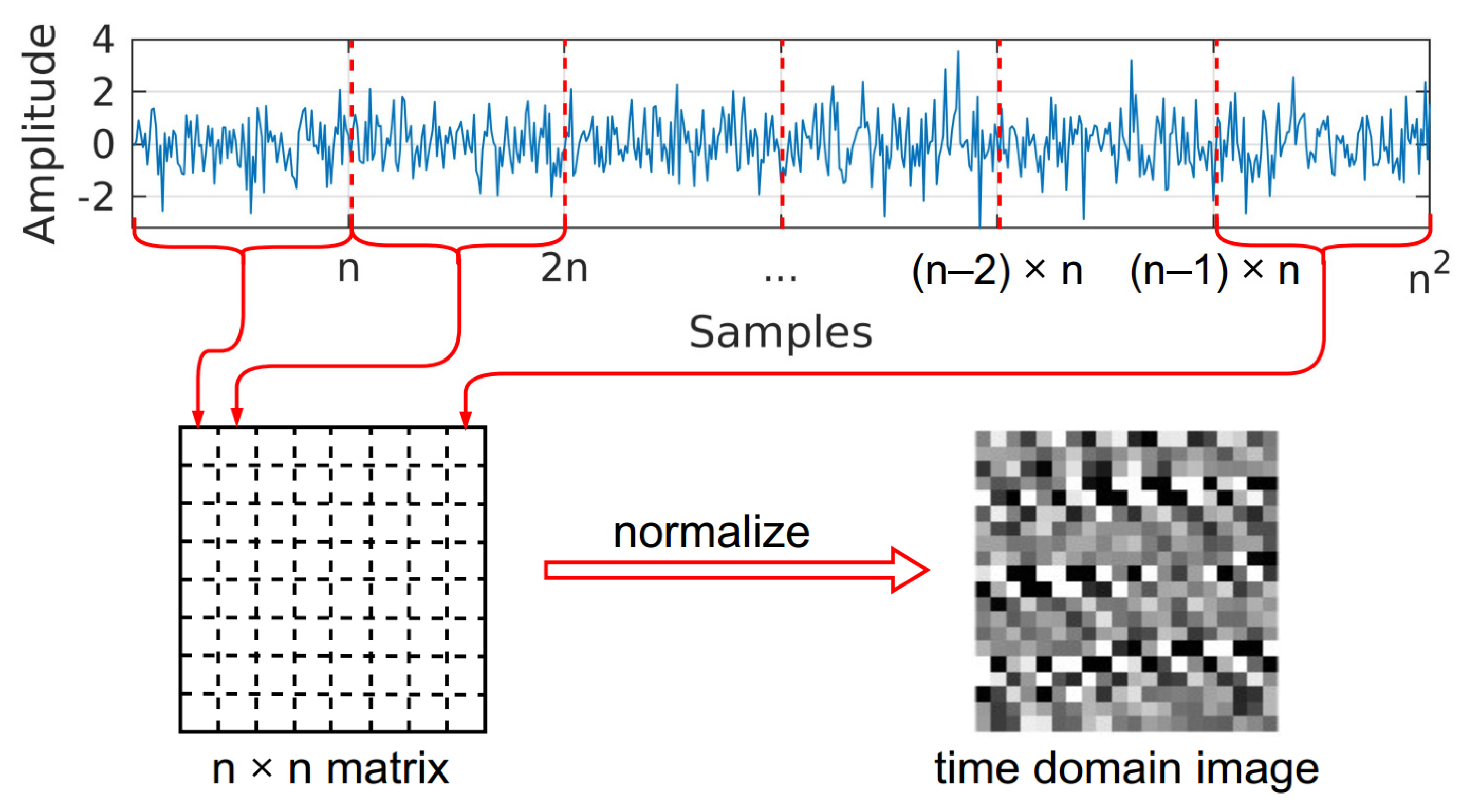
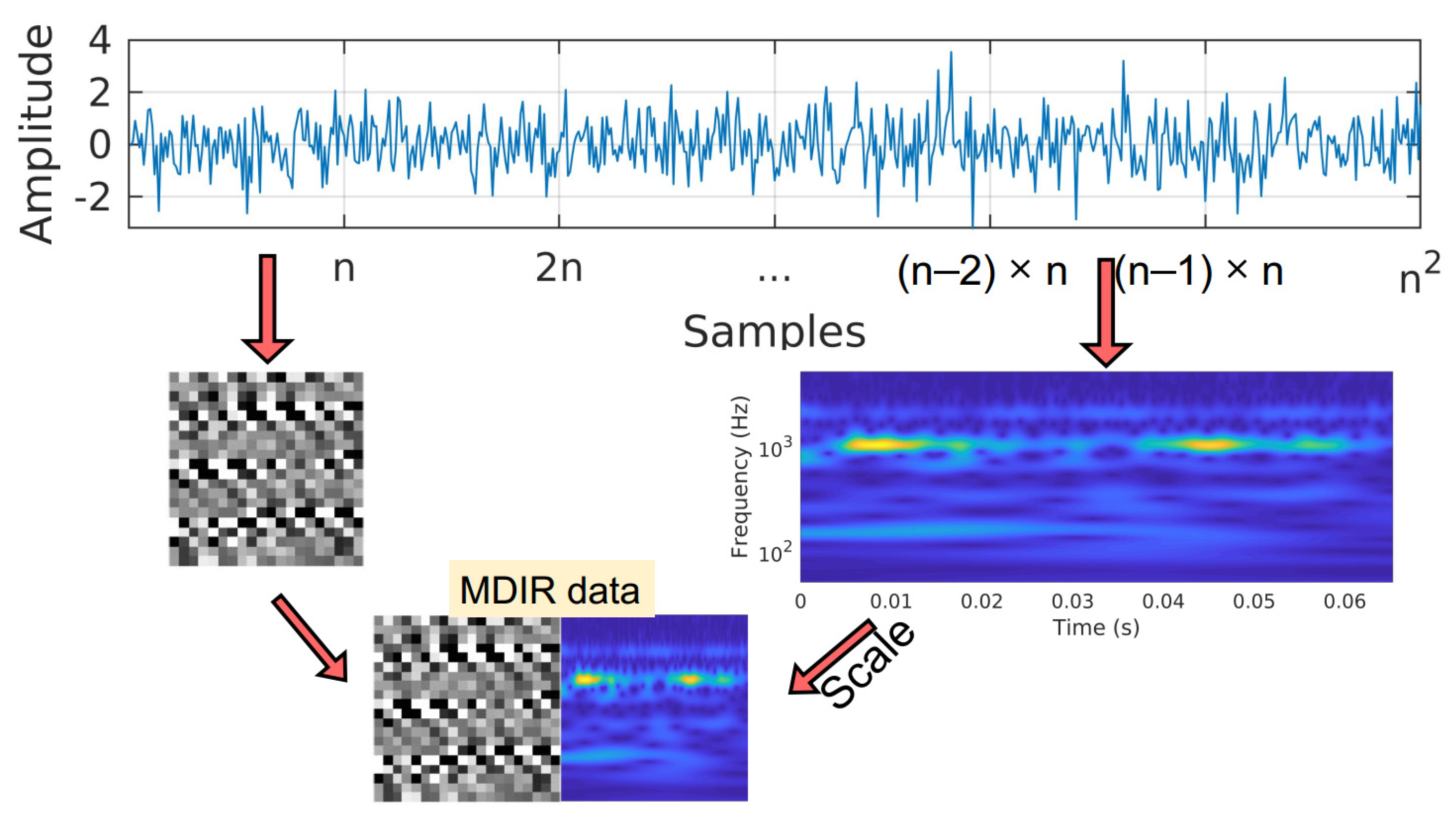
• Proposing a method to represent vibration signals in high dimensional form;
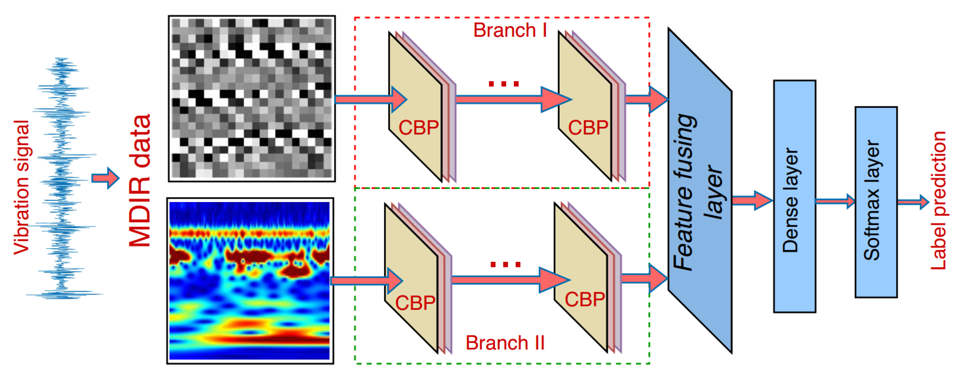
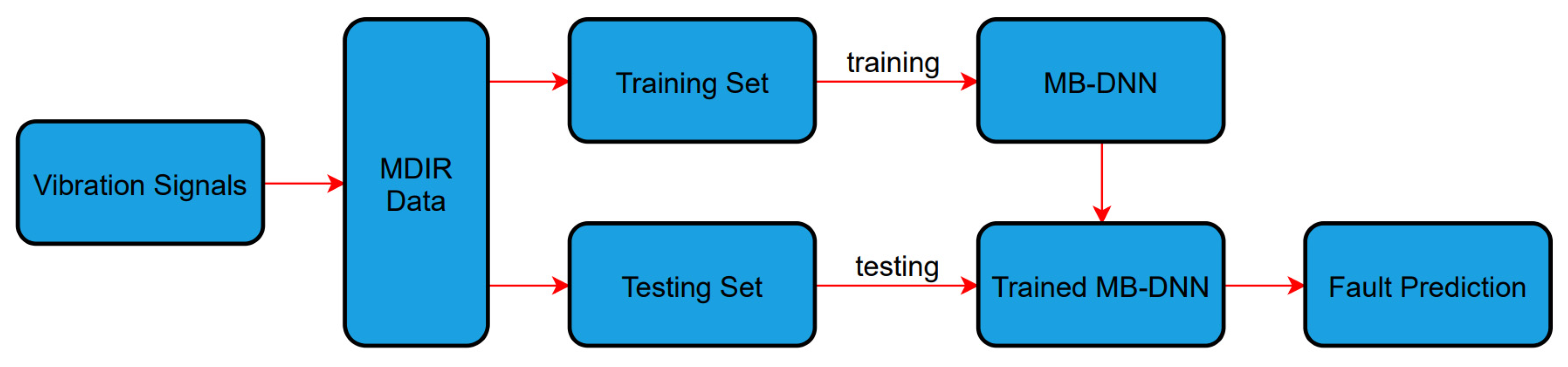
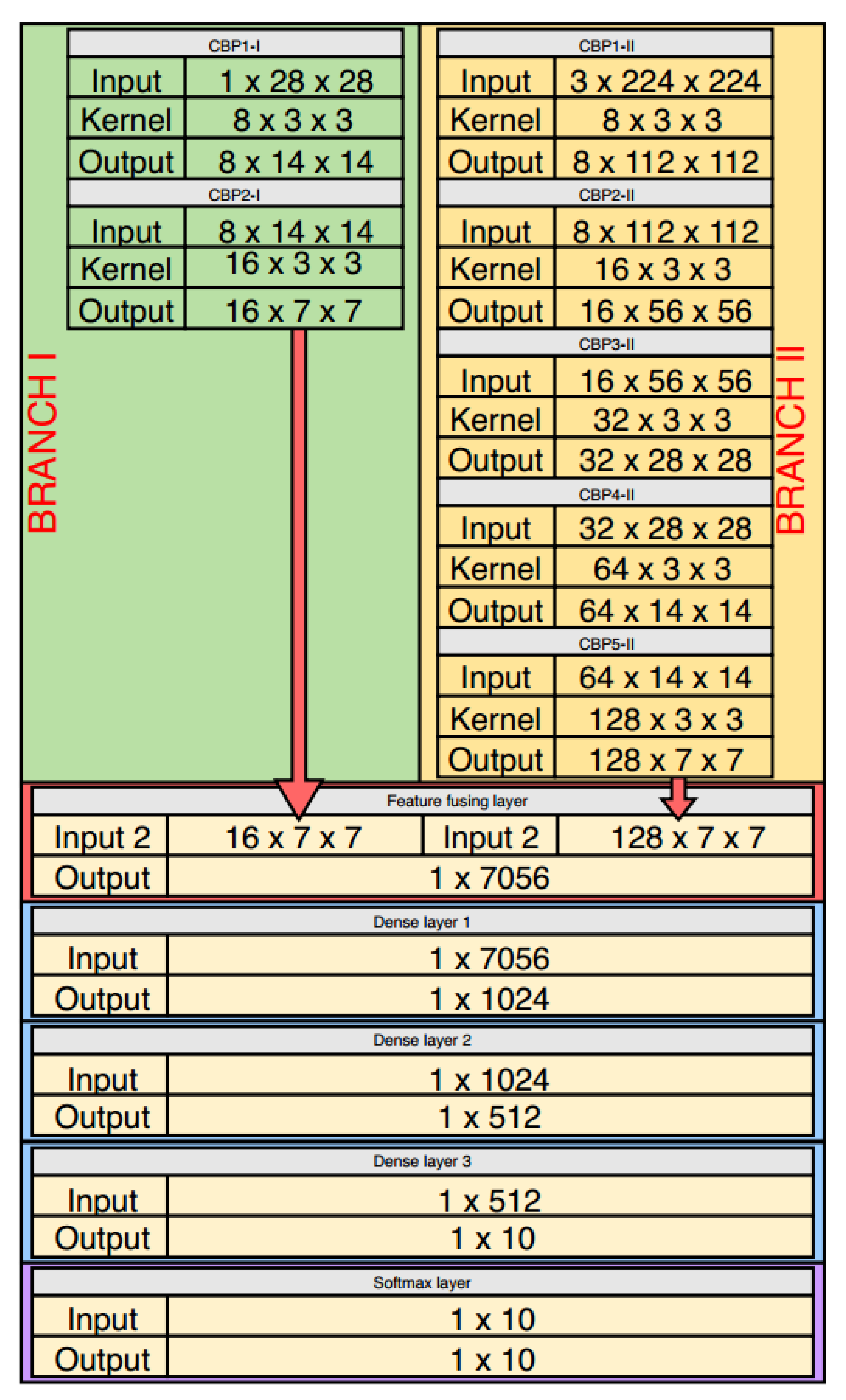
• Proposing an MB-DNN with a multi-branch structure to handle the new representation of vibration signal in the high-dimensional domain;
• Transforming the task of signal-based fault diagnosis into the task of image classification;
• The proposed fault diagnosis method achieves significant classification accuracy.

The remainder of the paper is constructed as follows. Section 2 describes the way of constructing MDIR data from vibration signals. Section 3 explains MB-DNN and its application in bearing fault diagnosis. Experiments with actual bearing data were conducted and are presented in Section 4. Section 5 concludes the paper.

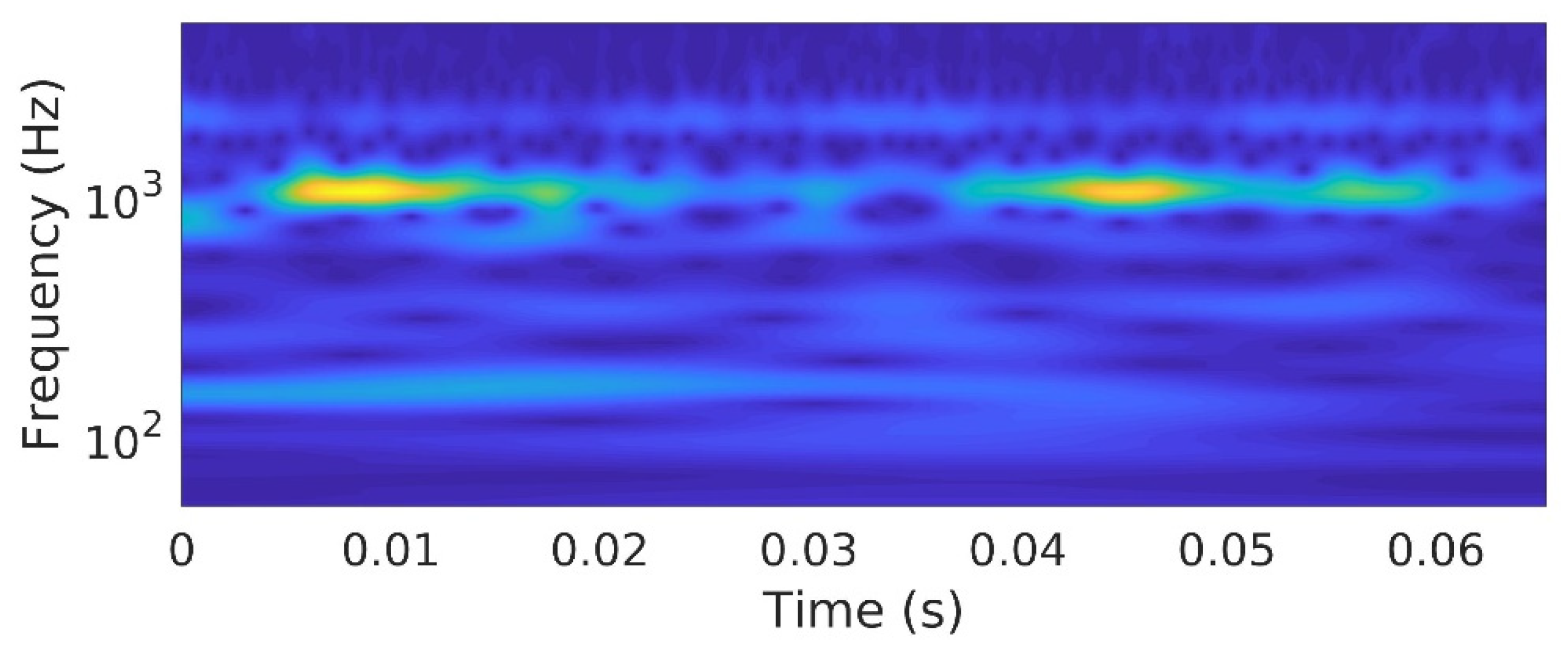
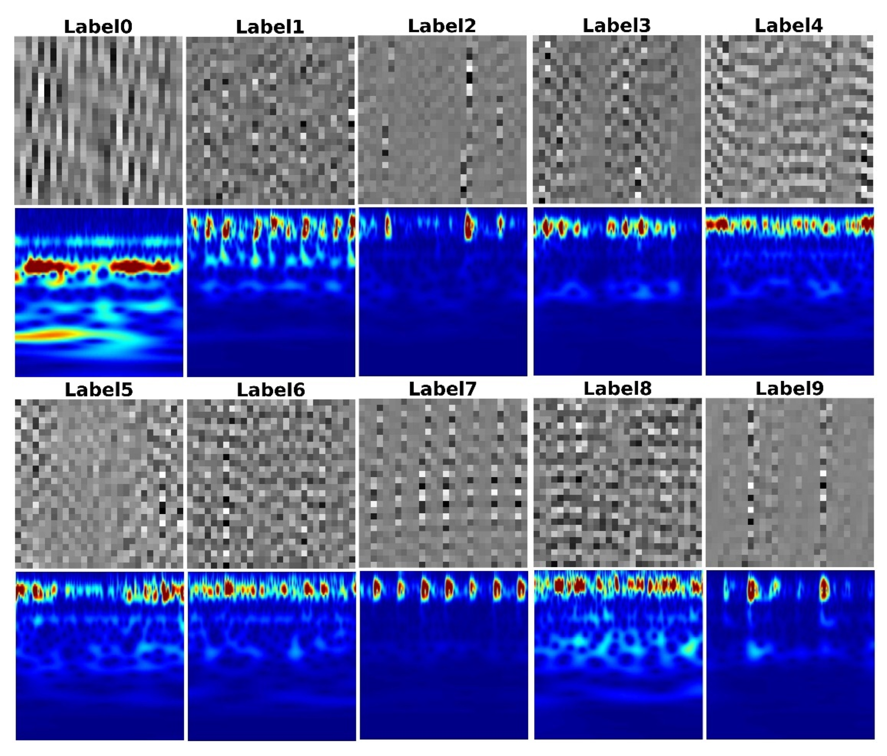
2. Multiple-Domain Image-Representation of Vibration Signal

Originally, vibration signal is time-series data, which is a 1-D data form. A new method to represent vibration signals in high dimensions is proposed. It is motivated by three following facts:

• It may be easier to understand and mine information in high-dimensional data [30].
• CNN and its variants are suitable for the task of recognizing two-dimensional visual patterns [31].
• By transforming the signal into visual data, the task of fault diagnosis can be converted into the task of image classification.

The vibration signal will be transformed into a time-domain image by a simple method proposed by D. Nguyen et al. in [32]. Consider a signal $x_l$ with the number of samples is $n^2$, all the samples in the signal are rearranged into a square matrix with a size of $n\times n$ as follows:

$$\left[\begin{array}{ccc}{x}_1& \dots & x_{n^2}\end{array}\right]\to \left[\begin{array}{cccc}{x}_1& x_2& \dots & x_n\\ x_{n+1}& x_{n+2}& \dots & x_{2n}\\ ⋮& ⋮& \ddots & ⋮\\ x_{\left(n-1\right)n+1}& \dots & \dots & x_{n^2}\end{array}\right]$$

(1)

Then the obtained square matrix is normalized to range $\left[0.0-1.0\right]$ by the linear normalization:

$$I_{ij}=\frac{X_{ij}-min\left(X\right)}{max\left(X\right)-min\left(X\right)}$$

(2)

The normalized sample $I_{ij}, i, j\in \left[0, n\right]$ is placed at the row $i$, column $j$ of the matrix. The corresponding time domain image consists of pixels that are normalized samples of the corresponding signal, as shown in Figure 1.

The time-frequency image representation is based on the continuous wavelet transform (CWT). The CWT uses the same length of time data as in the previous transformation. A mother wavelet is a function $\psi (t)$ with zero average (i.e., ${\int }_{\mathrm{R}}\psi -0$), normalized (i.e., $\Vert \psi \Vert =1$), and centered in the neighborhood of $t=0$ [33]. Scaling $\psi (t)$ by a positive quantity $s$, and translating it by $y\in \mathbf{R}$, a wavelet family can be defined as:

$${\psi }_{u,s}(t):=\frac{1}{\sqrt{s}}\psi \left(\frac{t-u}{s}\right), u\in \mathbf{R}, s>0$$

(3)

Given $x(t)\in L^2(\mathbf{R})$, the continuous wavelet transform of $x(t)$ at time $u$ and scale $s$ (which inversely relates to frequency) is defined as:

$$W(s,u):=\langle x(t), {\psi }_{s,u}\rangle =\frac{1}{\sqrt{s}}\int x\left(t\right)\psi *\left(\frac{t-u}{s}dt\right)$$

(4)

where $\psi *$ denotes the complex conjugate of $\psi$. CWT decomposes the input signal $x(t)$ into a series of wavelet coefficients. The scalogram of $x(t)$ is defined by the function:

$$\mathbf{S}(s):=\Vert W(s,u)\Vert =\sqrt{{{\int }_{-\infty }^{+\infty }\left|W(s,u)\right|}^{2}du}$$

(5)

If a time interval $\left[t_0, t_1\right]$ needs to be considered, the corresponding windowed scalogram is defined by the function:

$${\mathbf{S}}_{\left[t_0, t_1\right]}(s):={\Vert W(s,u)\Vert }_{\left[t_0, t_1\right]}=\sqrt{{{\int }_{t_0}^{t_1}\left|W(s,u)\right|}^{2}du}$$

(6)

In other words, the scalogram is the absolute value of the CWT of a signal, plotted as a function of time and frequency, as shown in Figure 2.

By combining two transformations, each vibration signal is transformed simultaneously into image form: the time domain image and the time-frequency domain image as shown in Figure 3. This representation of vibration signal is named multiple-domain image-representation (MDIR). By using MDIR data, the problem of fault diagnosis based on vibration signal can now be considered as a task of image classification.

3. Proposed Multi-Branch Deep Neural Network

In the previous section, the multiple-domain image-representation (MDIR) of vibration signal has been described. To handle the MDIR data, a multi-branch deep neural network (MB-DNN) is proposed. The structure of MB-DNN is shown in Figure 4.

The proposed MB-DNN consists of several types of layers, including convolutional layer, batch normalization layer, pooling layer, feature fusing layer, dense layers, and SoftMax layer.

The convolutional layer based on the convolution operation is the most important layer type, which has been employed in many well-known DNN models such as LeNet [34], AlexNet [35], VGGNet [36], ResNet [37], and DenseNet [38]. The convolutional layer convolves the input with its kernels and feeds the obtained result into the activate function to generate the output. Consider a convolutional layer with $m$ kernels, the input has $M$ feature maps. The output of that layer can be calculated as follows:

$$y_k=\mathit{f}\left({\displaystyle \sum _{i=1}^M{\omega }_k\otimes x_i+b_k}\right), k=1:m$$

(7)

where $\mathit{f}$ denotes the activate function. In this paper, the Rectified Linear Unit (ReLU) is used as the activate function since it is simple and easy to compute.

The batch normalization layer exploited the batch normalization technique proposed in [39] to improve the training process of DNNs. The batch normalization ensures the transformation inserted in the network by representing the identity transform. The pooling layer reduces the dimension of the input feature maps. The dimension reduction operation can be conducted by max or average operation. The pooling layer computes the max value or average value of a group of neurons at the previous layer.

For convenience in calling and easer in drawing the neural network structure, three layers, including one convolutional layer, one batch normalization layer, and one pooling layer, are grouped successively to construct a convolutional–batch normalization–pooling (CBP) module. Assume that a CBP module with a convolutional layer with $m$ kernels. With the input feature map $x^{M\times n\times n}$, the output of the CBP module will be $y^{m\times h\times h}$ where $h=n/2$.

As shown in Figure 4, the proposed MB-DNN has two branches. While branch I handles the time domain images, branch II handles the time-frequency domain images of the vibration signals. Each branch consists of several CBP modules. Two branches simultaneously extract features from the input MDIR data, generate two types of feature maps. After that, the feature fusing layer will fuse these feature maps to generate a single one and forward it to the next part of the network. The operation of the feature fusing layer is described as follows:

$$x=\mathit{C}\left(x_t,x_f\right)$$

(8)

where $\mathit{C}$ denotes the fusing operation of the layer; $x_t,x_f$ are the feature maps extracted by branch I and II, respectively. Assume that $x_t$ and $x_f$ has sizes $a_1\times \left(b_1\times b_1\right)$ and $a_2\times \left(b_2\times b_2\right)$, respectively. First, two feature maps will be flattened to have size $1\times \left(a_1\times b_1{}^2\right)$ and $1\times \left(a_2\times b_2{}^2\right)$, respectively. The output of this layer $x$ will have size $1\times \left(a_1\times b_1{}^2+a_2\times b_2{}^2\right)$.

The dense layer is a traditional perception neural network. The purpose of using a dense layer is to collect all features from the previous feature map. The generated feature map of this layer will be used for the classification task, which will be performed by the SoftMax layer. With an input feature map $x$, the SoftMax layer computes the probabilities:

$$p_r=\frac{\exp \left({\omega }_k\times x\right)}{{\displaystyle {\sum }_{r=1}^N\exp \left({\omega }_k\times x\right)}}$$

(9)

where $N$ is the number of classes in the classification task. The SoftMax function calculates the probabilities of each target class over all target classes.

The loss function of MB-DNN is calculated by cross-entropy loss as follows:

$$L\left(q,p\right)=-{\displaystyle \sum _r^N{q}_r\log (p_r)}$$

(10)

where $q$ is the true label of the input data, $p$ is the output of the SoftMax function.

Using the MDIR data and MB-DNN, the proposed fault diagnosis method is illustrated in Figure 5. As shown in the diagram, the original fault signals are transformed into MDIR data. Then the obtained dataset is split into a training set and a testing set. The MB-DNN is trained with the training set by the back-propagation algorithm. Using the stochastic gradient descent with momentum, the weights of MB-DNN are updated by the equations

$${\upsilon }_t=\beta {\upsilon }_{t-1}+(1-\beta ){\nabla }_{\omega }L$$

(11)

$$\omega =\omega -\alpha {\upsilon }_t$$

(12)

where $\alpha$ denotes the learning rate, $\alpha$ is the momentum parameter.

4. Experiments and Results

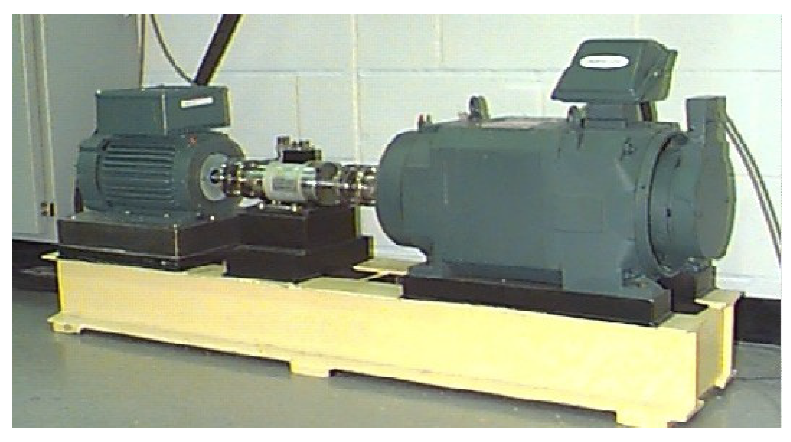
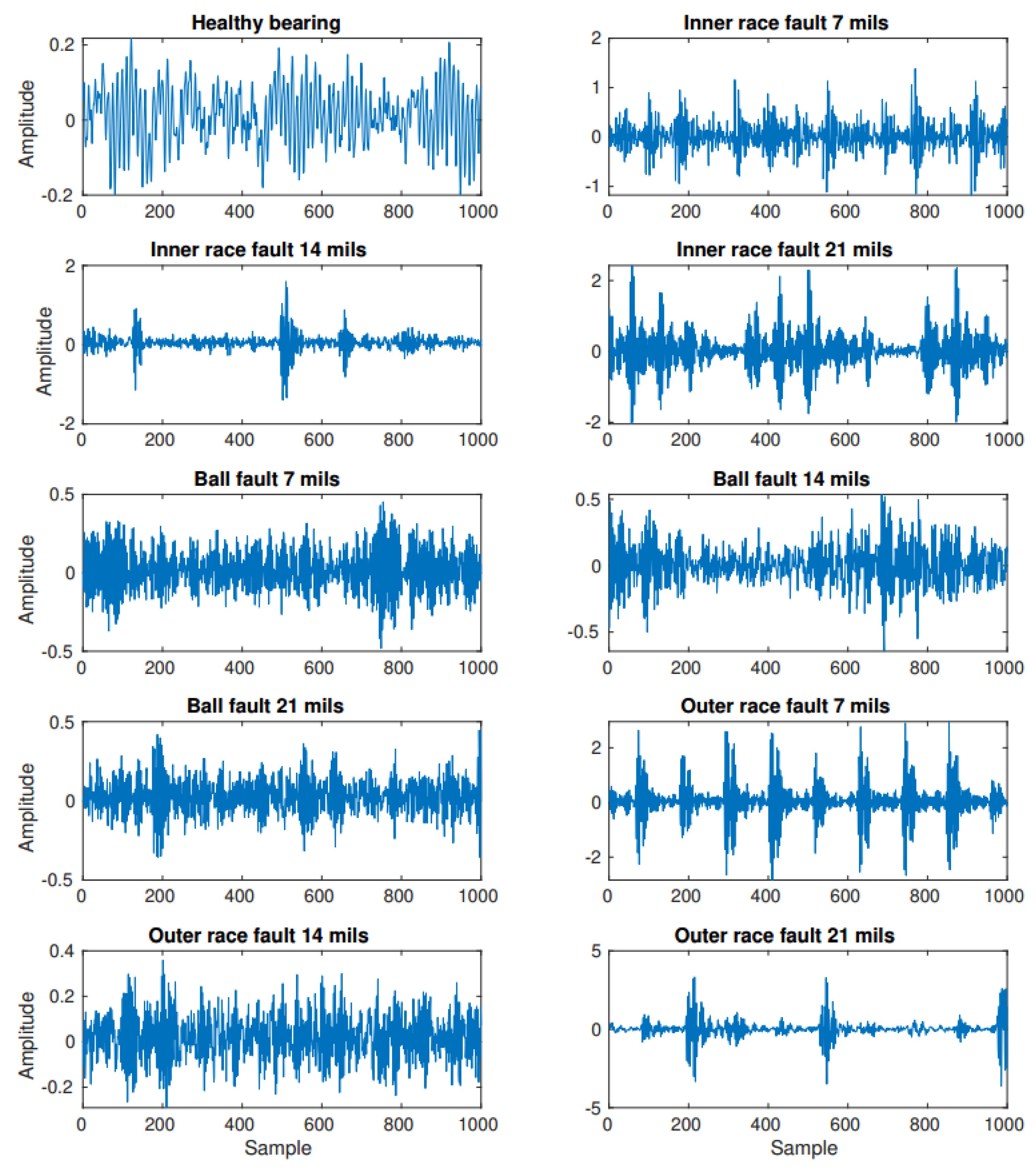
4.1. Data Preparation

The actual bearing fault data are supplied by the Bearing Data Center of Case Western Reserve University (CWRU) [40]. The bearing fault testbed is shown in Figure 6. The testbed consisted of a 2-hp motor (left), a torque transducer (center), and a dynamo-meter (right). The test bearings support the motor shaft. The test bearings were seeded with faults using electro-discharge machining (EMD).

The vibration signals in this paper are measured by an accelerometer and digitized with a sampling frequency of 12 kHz. The accelerometer is installed at the driver end with magnetic bases. There are four types of bearing conditions are considered, including no-fault condition, bearing with inner race fault, bearing with outer race fault, and bearing with fault at rolling elements (ball fault). Each type of bearing fault is introduced to the test bearings with different defect sizes, including 7 mils (mili-inches), 14 mils, and 21 mils. The types of bearing conditions with different fault diameters are shown in

Table 1. Vibration labels.

Bearing Fault	Fault Size (mils)	Label
No fault		0
Inner race fault	7	1
Inner race fault	14	2
Inner race fault	21	3
Ball fault	7	4
Ball fault	14	5
Ball fault	21	6
Outer race	7	7
Outer race	14	8
Outer race	21	9

and Figure 7. There are 10 types of bearing conditions labeled from 0 to 9, respectively. The bearing testbed can be operated under different load conditions. In this paper, four load conditions were considered, including 0 hp, 1 hp, 2 hp, and 3 hp.

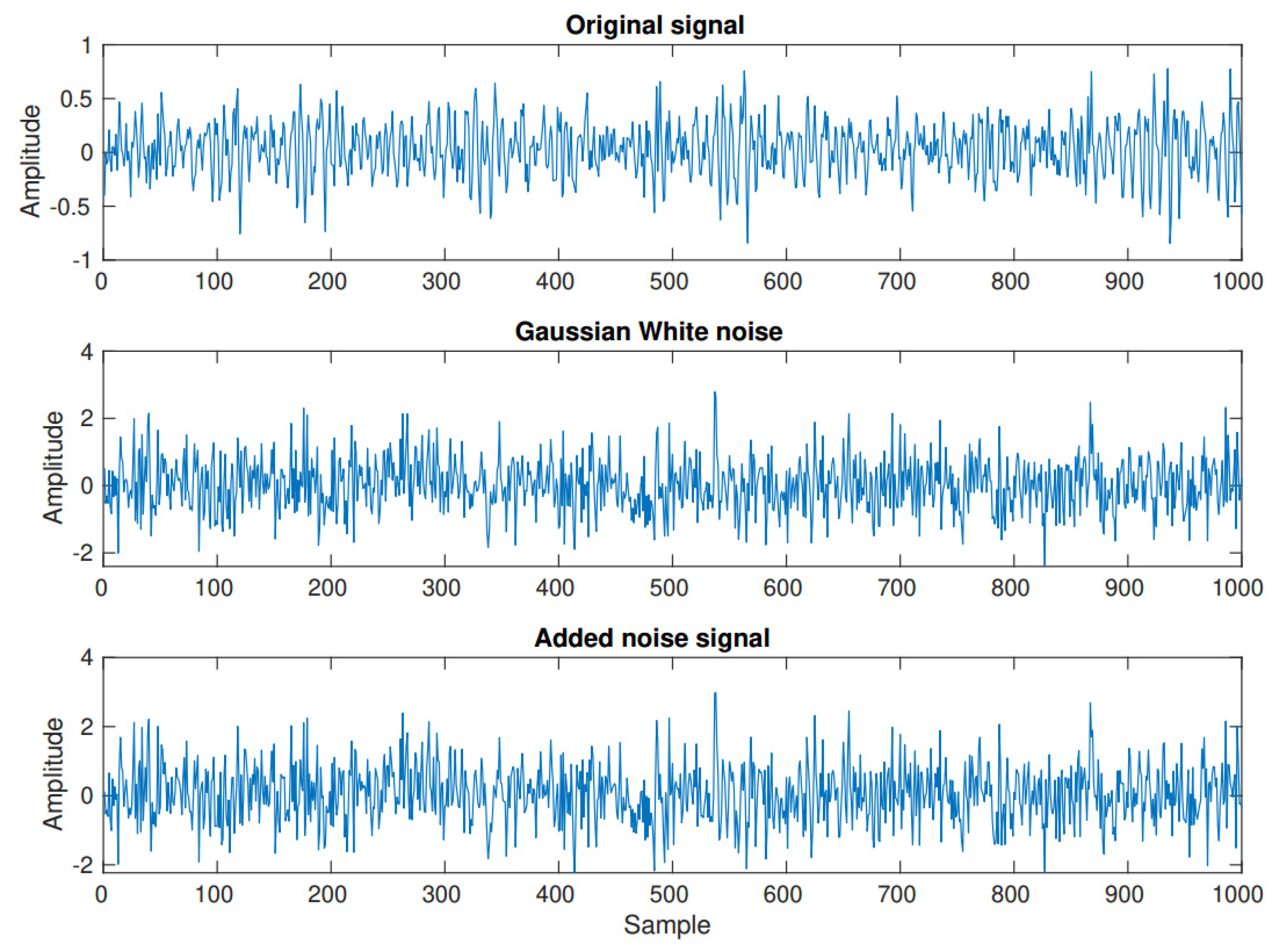
4.2. Signal Pre-Processing

In the data source supplied by CWRU, each bearing condition fault signal is measured and stored in a single file Matlab file; thus, there are 10 different signal files corresponding to 10 bearing conditions as in Table 1. In the intelligent fault diagnosis approach, classifiers require data samples to be trained; therefore, the original signal files are split into equal signal samples. Each signal sample must contain enough sampling points to convey the information of the bearing status; that is, if the length is too short, the signal sample cannot reflect the bearing health status. Normally, the sample length is selected to be equal to one revolution of the rotary shaft. In this work, the rotary speed of the shaft is $S=1796 \mathrm{rpm}$. Accordingly, the rotary frequency is $S_f=1796/60\approx 30 \mathrm{Hz}$. In the CWRU testbed, the sampling frequency $F=12,000 \mathrm{Hz}$. The minimum value of the sample length is $F/S_f=400$ (sampling point). As mentioned in Section 3, in the proposed method, there is a step where signal samples are transformed into gray images and apply CNN-like neural network to classify. So, we aim to make an MNIST-like data set where each image has a size of $1\times 28\times 28$; therefore, the length of signal samples is selected at the value of $28\times 28=784$. The time-domain image has the size of $1\times 28\times 28$.

The time-frequency domain image conversion exploits CWT using the Morse wavelet function. To deal with the time-frequency domain image, the obtained time-frequency images are scaled to a size of $3\times 224\times 224$. The MDIR data of the vibration signals with ten labels were obtained as shown in Figure 8.

From each original signal file, 300 data samples were obtained. Accordingly, the 10-class classification task is balanced since each class has 300 data samples. For each label, the image data were split randomly with the ratio 7:3 for the training set and the test set.

4.3. Design and Train the Proposed DNN

The structure of the proposed MB-DNN is designed as follows. First of all, the number of branches is two, corresponding to two types of input images. The input sizes of branches must be suitable for the input images; therefore, the first branch has the input size of $1\times 28\times 28$ and the second branch has the input size of $3\times 224\times 224$. The kernel size of convolutional layers and pooling layers are $3\times 3$ and $2\times 2$, respectively. The number of kernels in the convolutional layer is selected by a simple rule. Start with a small number of kernels in the first layer and double that number in the next layer. The first convolutional layer has 8 kernels, the second layer has 16 kernels, the third layer has 32 kernels, and so on. Each module CBP consists of one convolutional layer, one batch normalization layer, and one pooling layer. Since we use the zero-padding method in convolutional layers and the kernel size of $2\times 2$ in pooling layers, after each module CBP, the size of data will decrease by a factor of 2. The number of CBP modules is increased by one until the size of the output data is an odd number. In the first branch, two CBP modules are used; in the second branch, five CBP modules are used. The proposed MB-DNN has the configuration as shown in Figure 9. Branch I consists of two CPB modules that handle the time domain images. Branch II uses five CBP modules to handle the time-frequency domain images. The output of branch I has a size of $16\times 7\times 7$. The output of branch II has a size of $128\times 7\times 7$. These two outputs are fed into the feature fusing layer to generate the output data with size of $1\times 7056$. Then three successive dense layers are used to learn from the fused feature map. Finally, a SoftMax layer with ten outputs is used to classify the feature map generated by the third dense layer.

The MB-DNN is trained by mini-batch stochastic gradient descent with momentum algorithm, the learning rate $\alpha =0.001$, the momentum $\beta =0.9$, and the batch size $B=10$.

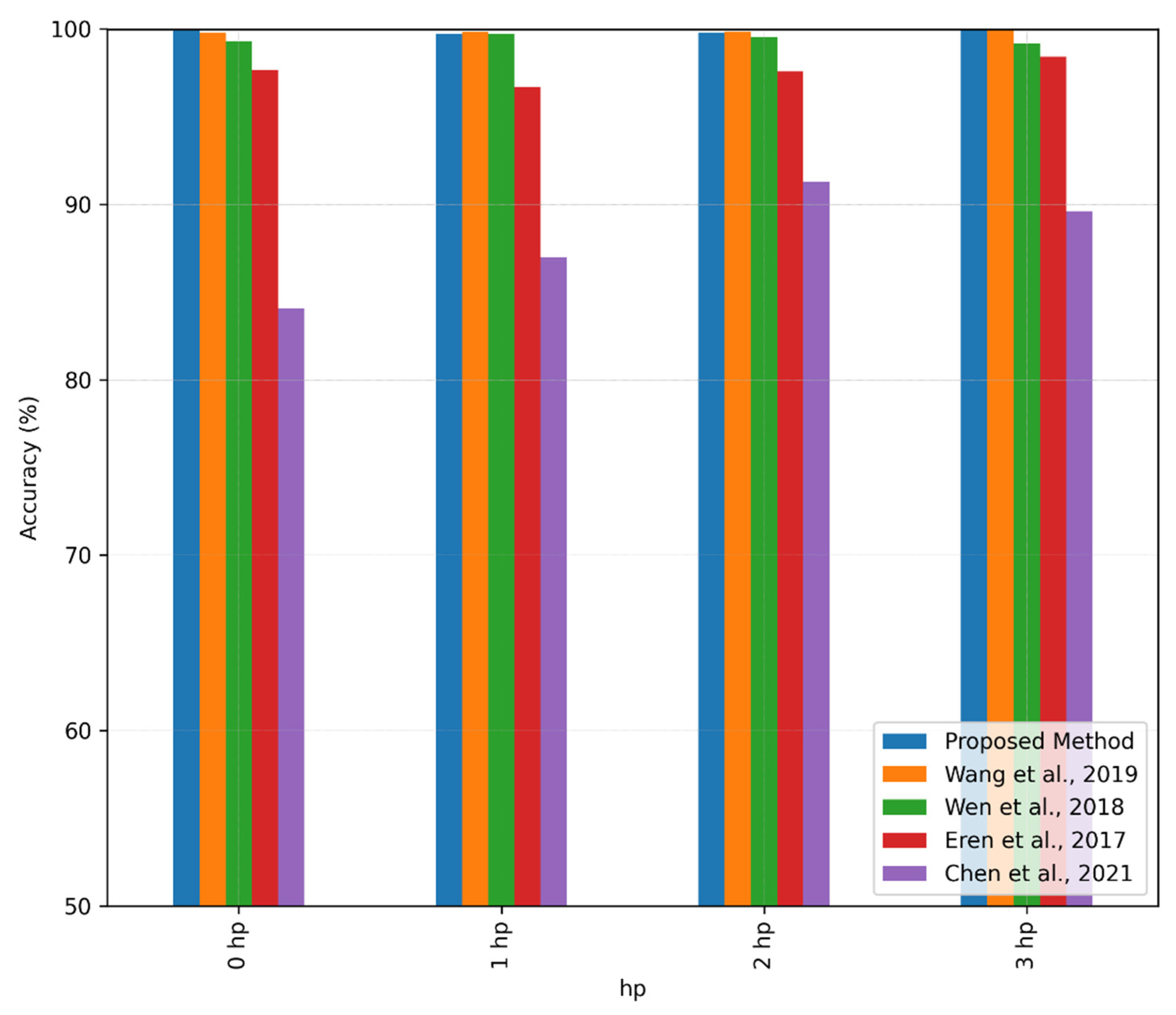
4.4. Fault Diagnosis Result

Four other bearing fault diagnosis methods are adopted to make comparisons with the proposed method as follows. The first method is published in [25]. In this method, the deep transfer learning technique is utilized to transfer the very deep neural network (Alexnet) pre-trained in the image classification domain into the domain of bearing fault diagnosis. The vibration signals are transformed into image form by using CWT. The second method is published in [24]. This method uses Lenet-5, which is a classical type of CNN in [41]. In this method, each sample of vibration signal is rearranged into a square matrix. The third method is published in [26]. This method utilized the 1-D form of CNN, which can process the vibration signal samples directly in the 1-D form without any transformation. The fourth method is published in [42]. The same as the method in [26], the vibration signals in [42] are used directly in 1-D form without any transformation. However, the number of convolution kernels of CNN is decreased with the reduction in the convolution kernel size.

The accuracy of all methods is shown in Figure 10. It can be observed that in all cases of load conditions, the proposed method and the Alexnet-based method in [25] achieve the best performance. The two methods have high mean accuracy and small standard deviation. The Lenet5-based method in [24] has a little lower accuracy. The CNN1D-based method in [26] has a lower performance with low accuracy. The CNN1D-based method in [42] has the poorest performance with low accuracy.

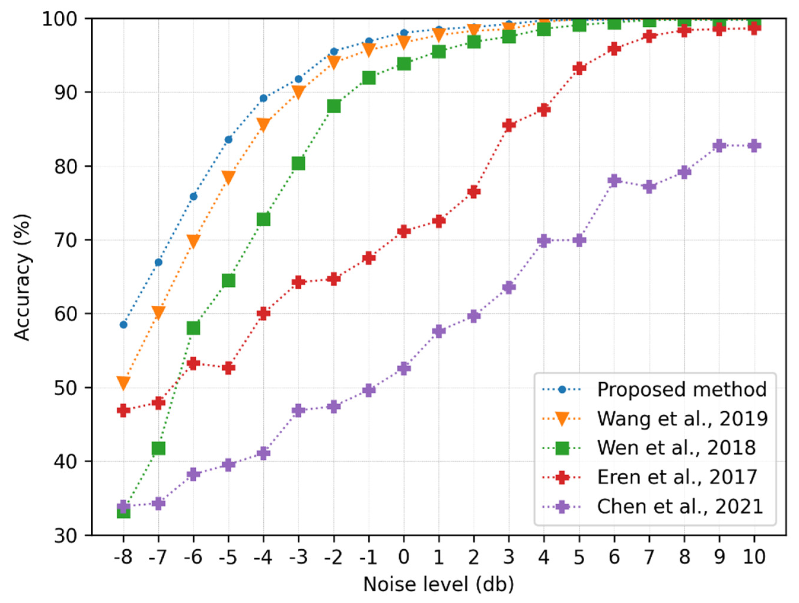
4.5. Evaluation under Noisy Conditions

The bearing data set supplied by CWRU has been extensively employed as a benchmark for evaluating bearing fault diagnosis methods. Recently, proposed fault diagnosis methods with advantage signal processing and feature learning techniques can achieve very high accuracy. It is not easy to highlight the performance of newly proposed fault diagnosis methods; therefore, noise signals are often added to the original signals to evaluate methods. This way can help to evaluate the robustness of fault diagnosis methods under more challenging conditions. In this scenario of evaluating diagnosis methods, Gaussian white noise (AGWN) is added into the original vibration signals as in Figure 11.

The signal-to-noise ratio (SNR) is defined to measure the level of the obtained noisy signal to the level of the additional Gaussian noise. The SNR of a noisy signal is computed as follows:

$$\mathrm{SNM}=10\log \left(\frac{{\mathrm{P}}_{\mathrm{signal}}}{{\mathrm{P}}_{\mathrm{noise}}}\right)$$

(13)

where ${\mathrm{P}}_{\mathrm{signal}}$ and ${\mathrm{P}}_{\mathrm{noise}}$ are the power of signal and noise, respectively. Nineteen noise levels (dB) in the range of [−8, −7, …, 10] are taken into account. The comparison is illustrated in Figure 12.

In the previous section, all compared methods achieved very high diagnostic accuracy when the inputs were the original signals. When the input signals were transformed by adding low-level noisy signals with the SNR in the range of [0, …, 10], the performance of the method in [26,42] was significantly reduced, but the performance of the proposed algorithm and the methods in [24,25] were reduced insignificantly; however, when the input signals are transformed by adding high-level noisy signals with the SNR in the range of [−8, …, −1], their performance decreases dramatically. Obviously, the noise makes it harder to extract fault signatures from the signals. It can be observed that in the worst case (−8 dB), the methods in [24,26,42] totally fail since their accuracy is under 50%. The trend of all methods’ performance is, the higher the noise level, the lower the accuracy of the diagnosis result. Among all methods, the proposed one achieves the best performance with good robustness against noise. Even under the worst noise case (−8 dB), it achieves an accuracy of 57%. Comparing the structures of all methods, we can see that the method in [25] only takes care of the time-frequency domain features; the methods in [24,26,42] only consider the time domain features. The difference of the proposed methods is that they can receive multiple feature domains. As a result, the proposed method can extract more robust features from signals in noise conditions. So, it can be concluded that the proposed network with a multi-branch deep structure can extract fault features more effectively even under severe noise conditions. That leads to better diagnostic performance compared to other DNNs.

5. Conclusions

This paper proposed a novel method of bearing fault diagnosis based on vibration signals. By using simple transformation methods, time-series vibration signals are transformed into high dimensional data form (MDIR). By using this transformation, the task of fault diagnosis becomes the task of image classification. A novel DNN with a multi-branch structure is proposed to handle the MDIR data of vibration signal, named MB-DNN. The proposed MB-DNN inherits the advantages of CNN in processing high-dimensional data. In addition, MB-DNN has a multi-branch structure with two branches that can simultaneously extract features from the time domain and time-frequency domain. The proposed method obtains high classification accuracy; especially, it shows the efficiency even under noise effects. The proposed algorithm can be applied as an automatic fault detection process for the early detection of bearing faults; therefore, it helps to reduce the failure rate of machinery and save repair costs. Besides the ability to process vibration signals, the proposed method can be applied to process the current signals and acoustic emission signals.

References

1. Shahriar, M.R.; Borghesani, P.; Tan, A.C.C. Electrical signature analysis-based detection of external bearing faults in electromechanical drivetrains. IEEE Trans. Ind. Electron. 2017, 65, 5941–5950. [Google Scholar] [CrossRef]
2. Van, M.; Hoang, D.T.; Kang, H.J. Bearing fault diagnosis using a particle swarm optimization-least squares wavelet support vector machine classifier. Sensors 2020, 20, 3422. [Google Scholar] [CrossRef] [PubMed]
3. Hoang, D.T.; Tran, X.T.; Van, M.; Kang, H.J. A Deep Neural Network-Based Feature Fusion for Bearing Fault Diagnosis. Sensors 2021, 21, 244. [Google Scholar] [CrossRef] [PubMed]
4. Xu, G.; Hou, D.; Qi, H.; Bo, L. High-speed train wheel set bearing fault diagnosis and prognostics: A new prognostic model based on extendable useful life. Mech. Syst. Signal. Proc. 2021, 146, 107050. [Google Scholar] [CrossRef]
5. Azamfar, M.; Singh, J.; Bravo-Imaz, I.; Lee, J. Multisensor data fusion for gearbox fault diagnosis using 2-D convolutional neural network and motor current signature analysis. Mech. Syst. Signal. Proc. 2020, 144, 106861. [Google Scholar] [CrossRef]
6. Hoang, D.T.; Kang, H.J. A motor current signal-based bearing fault diagnosis using deep learning and information fusion. IEEE Trans. Instrum. Meas. 2019, 69, 3325–3333. [Google Scholar] [CrossRef]
7. Kharche, P.P.; Kshirsagar, S.V. Review of fault detection in rolling element bearing. Int. J. Innov. Res. Adv. Eng. 2014, 1, 169–174. [Google Scholar]
8. Rauber, T.W.; de Assis Boldt, F.; Varejão, F.M. Heterogeneous feature models and feature selection applied to bearing fault diagnosis. IEEE Trans. Ind. Electron. 2014, 62, 637–646. [Google Scholar] [CrossRef]
9. Li, C.; Sanchez, V.; Zurita, G.; Lozada, M.C.; Cabrera, D. Rolling element bearing defect detection using the generalized synchrosqueezing transform guided by time--frequency ridge enhancement. ISA Trans. 2016, 60, 274–284. [Google Scholar] [CrossRef]
10. Zhou, D.-X. Universality of deep convolutional neural networks. Appl. Comput. Harmon. Anal. 2020, 48, 787–794. [Google Scholar] [CrossRef] [Green Version]
11. Li, X.; Zhang, W.; Ma, H.; Luo, Z.; Li, X. Degradation Alignment in Remaining Useful Life Prediction Using Deep Cycle-Consistent Learning. IEEE Trans. Neural Netw. Learn. Syst. 2021, 1–12. [Google Scholar] [CrossRef] [PubMed]
12. Saravanakumar, R.; Krishnaraj, N.; Venkatraman, S.; Sivakumar, B.; Prasanna, S.; Shankar, K. Hierarchical symbolic analysis and particle swarm optimization based fault diagnosis model for rotating machineries with deep neural networks. Measurement 2021, 171, 108771. [Google Scholar] [CrossRef]
13. Alabsi, M.; Liao, Y.; Nabulsi, A.-A. Bearing fault diagnosis using deep learning techniques coupled with handcrafted feature extraction: A comparative study. J. Vib. Control. 2021, 27, 404–414. [Google Scholar] [CrossRef]
14. Choudhary, A.; Mian, T.; Fatima, S. Convolutional neural network based bearing fault diagnosis of rotating machine using thermal images. Measurement 2021, 176, 109196. [Google Scholar] [CrossRef]
15. Wang, C.; Xu, Z. An intelligent fault diagnosis model based on deep neural network for few-shot fault diagnosis. Neurocomputing 2021, 456, 550–562. [Google Scholar] [CrossRef]
16. LeCun, Y.; Ranzato, M. Deep learning tutorial. In Proceedings of the Tutorials in International Conference on Machine Learning (ICML’13), Atlanta, GA, USA, 16–21 June 2013; pp. 1–29. [Google Scholar]
17. Nguyen, C.D.; Prosvirin, A.E.; Kim, C.H.; Kim, J.-M. Construction of a sensitive and speed invariant gearbox fault diagnosis model using an incorporated utilizing adaptive noise control and a stacked sparse autoencoder-based deep neural network. Sensors 2021, 21, 18. [Google Scholar] [CrossRef] [PubMed]
18. Salimans, T.; Goodfellow, I.; Zaremba, W.; Cheung, V.; Radford, A.; Chen, X. Improved techniques for training gans. Adv. Neural Inf. Proc. Syst. 2016, 29, 2234–2242. [Google Scholar]
19. Pham, M.T.; Kim, J.-M.; Kim, C.H. Efficient Fault Diagnosis of Rolling Bearings Using Neural Network Architecture Search and Sharing Weights. IEEE Access 2021, 9, 98800–98811. [Google Scholar] [CrossRef]
20. Zan, T.; Wang, H.; Wang, M.; Liu, Z.; Gao, X. Application of multi-dimension input convolutional neural network in fault diagnosis of rolling bearings. Appl. Sci. 2019, 9, 2690. [Google Scholar] [CrossRef] [Green Version]
21. Pham, M.-T.; Kim, J.-M.; Kim, C.-H. 2D CNN-Based Multi-Output Diagnosis for Compound Bearing Faults under Variable Rotational Speeds. Machines 2021, 9, 199. [Google Scholar] [CrossRef]
22. Wei, Y.; Xia, W.; Lin, M.; Huang, J.; Ni, B.; Dong, J.; Zhao, Y.; Yan, S. HCP: A flexible CNN framework for multi-label image classification. IEEE Trans. Pattern Anal. Mach. Intell. 2015, 38, 1901–1907. [Google Scholar] [CrossRef] [PubMed] [Green Version]
23. Cao, X.; Yao, J.; Xu, Z.; Meng, D. Hyperspectral image classification with convolutional neural network and active learning. IEEE Trans. Geosci. Remote Sens. 2020, 58, 4604–4616. [Google Scholar] [CrossRef]
24. Wen, L.; Li, X.; Gao, L.; Zhang, Y. A New Convolutional Neural Network-Based Data-Driven Fault Diagnosis Method. IEEE Trans. Ind. Electron. 2018, 65, 5990–5998. [Google Scholar] [CrossRef]
25. Wang, J.; Mo, Z.; Zhang, H.; Miao, Q. A deep learning method for bearing fault diagnosis based on time-frequency image. IEEE Access 2019, 7, 42373–42383. [Google Scholar] [CrossRef]
26. Eren, L. Bearing fault detection by one-dimensional convolutional neural networks. Math. Probl. Eng. 2017, 2017, 1–9. [Google Scholar] [CrossRef] [Green Version]
27. Jia, F.; Lei, Y.; Lin, J.; Zhou, X.; Lu, N. Deep neural networks: A promising tool for fault characteristic mining and intelligent diagnosis of rotating machinery with massive data. Mech. Syst. Signal. Proc. 2016, 72, 303–315. [Google Scholar] [CrossRef]
28. Yuan, L.; Lian, D.; Kang, X.; Chen, Y.; Zhai, K. Rolling bearing fault diagnosis based on convolutional neural network and support vector machine. IEEE Access 2020, 8, 137395–137406. [Google Scholar] [CrossRef]
29. Smith, W.A.; Randall, R.B. Rolling element bearing diagnostics using the Case Western Reserve University data: A benchmark study. Mech. Syst. Signal. Proc. 2015, 64, 100–131. [Google Scholar] [CrossRef]
30. Ding, X.; He, Q. Energy-fluctuated multiscale feature learning with deep convnet for intelligent spindle bearing fault diagnosis. IEEE Trans. Instrum. Meas. 2017, 66, 1926–1935. [Google Scholar] [CrossRef]
31. Phung, S.L.; Bouzerdoum, A. Visual and Audio Signal Processing Lab. University of Wollongong. 2009. Available online: https://documents.uow.edu.au/~phung/docs/cnn-matlab/cnn-matlab.pdf (accessed on 9 December 2021).
32. Nguyen, D.; Kang, M.; Kim, C.-H.; Kim, J.-M. Highly reliable state monitoring system for induction motors using dominant features in a two-dimension vibration signal. New Rev. Hypermedia Multimed. 2013, 19, 248–258. [Google Scholar] [CrossRef]
33. Bolós, V.J.; Ben’itez, R. The wavelet scalogram in the study of time series. In Advances in Differential Equations and Applications; Springer: Berlin/Heidelberg, Germany, 2014; pp. 147–154. [Google Scholar]
34. LeCun, Y.; Haffner, P.; Bottou, L.; Bengio, Y. Object recognition with gradient-based learning. In Shape, Contour and Grouping in Computer Vision; Springer: Berlin/Heidelberg, Germany, 1999; pp. 319–345. [Google Scholar]
35. Krizhevsky, A.; Sutskever, I.; Hinton, G.E. Imagenet classification with deep convolutional neural networks. Adv. Neural Inf. Proc. Syst. 2012, 25, 1097–1105. [Google Scholar] [CrossRef]
36. Simonyan, K.; Zisserman, A. Very deep convolutional networks for large-scale image recognition. arXiv 2014, arXiv:1409.1556. [Google Scholar]
37. He, K.; Zhang, X.; Ren, S.; Sun, J. Deep residual learning for image recognition. In Proceedings of the IEEE Conference on Computer Vision and Pattern Recognition, Las Vegas, NV, USA, 27–30 June 2016; pp. 770–778. [Google Scholar]
38. Huang, G.; Liu, Z.; Van Der Maaten, L.; Weinberger, K.Q. Densely connected convolutional networks. In Proceedings of the IEEE Conference on Computer Vision and Pattern Recognition, Honolulu, HI, USA, 21–26 July 2017; pp. 4700–4708. [Google Scholar]
39. Ioffe, S.; Szegedy, C. Batch normalization: Accelerating deep network training by reducing internal covariate shift. In Proceedings of the International Conference on Machine Learning, Lille, France, 6–11 July 2015; pp. 448–456. [Google Scholar]
40. Loparo, K.A. Case Western Reserve University Bearing Data Center. Available online: http://csegroups.case.edu/bearingdatacenter/pages/download-data-file (accessed on 9 December 2021).
41. LeCun, Y.; Bottou, L.; Bengio, Y.; Haffner, P. Gradient-based learning applied to document recognition. Proc. IEEE 1998, 86, 2278–2324. [Google Scholar] [CrossRef] [Green Version]
42. Chen, C.-C.; Liu, Z.; Yang, G.; Wu, C.-C.; Ye, Q. An Improved Fault Diagnosis Using 1D-Convolutional Neural Network Model. Electronics 2021, 10, 59. [Google Scholar] [CrossRef]
Figure 1. Time domain image transformation.
Machines 09 00345 g001
Figure 2. Scalogram of the vibration signal.
Machines 09 00345 g002
Figure 3. MDIR data of vibration signal.
Machines 09 00345 g003
Figure 4. Multi-branch deep neural network.
Machines 09 00345 g004
Figure 5. Diagram of proposed bearing fault diagnosis method.
Machines 09 00345 g005
Figure 6. Bearing fault testbed used by CWRU.
Machines 09 00345 g006
Figure 7. Vibration signals.
Machines 09 00345 g007
Figure 8. MDIR data of vibration signals.
Machines 09 00345 g008
Figure 9. Configuration of MB-DNN.
Machines 09 00345 g009
Figure 10. Mean accuracy (%) of methods under different load conditions.
Machines 09 00345 g010
Figure 11. Noise signal.
Machines 09 00345 g011
Figure 12. Diagnosis accuracy of four methods under different noise levels (load condition: 2 hp).
Machines 09 00345 g012