Formation Control of Dual Auto Guided Vehicles Based on Compensation Method in 5G Networks

Abstract

With commercial application of 5G networks, many researchers have started paying attention to real-time control in 5G networks. This paper focuses on dual auto guided vehicles collaborative transport scenarios and designs a formation control system in current commercial 5G networks. Firstly, the structure of the 5G network researched in this paper is introduced. Then the round-trip time of 5G networks is measured and analyzed. The result shows that although the 5G round-trip time has randomness, it is mainly concentrated in 19 ± 3 ms, and the jitter mainly in 0 ± 3 ms. The Kalman filter is applied to estimate the transmission delay and experiment result shows the effectiveness of the estimation. Furthermore, the total delay including transmission delay and execution delay in control system is discussed. After establishing the AGV kinematic and formation model, complete control system based on compensation method is proposed. Finally, an experiment is carried out. Compared to the result without formation control, maximum distance error is reduced by 82.61% on average, while maximum angle error 45.91% on average. The result shows the effectiveness of the control system in formation maintaining in 5G network.

1. Introduction

As the new generation communication technology, 5G networks have gained vital development and attention in recent years. International Telecommunication Union (ITU) has defined three typical scenarios for 5G: enhanced Mobile Broadband (eMBB), massive Machine Type Communications (mMTC), and ultra-Reliable Low Latency Communication (uRLLC). The 3rd Generation Partnership Project (3GPP) has developed specifications for 5G New Radio and finished the 5G standards Release 15 (5G R15) in June 2018. As the first full set standard of 5G, 5G R15 has been commercialized and available for individuals and businesses. Nowadays, academia and industry are widely recognized that 5G has significant potential in industry application and is the key wireless technology in Industry 4.0 [1]. Many companies have applied 5G R15 to their intelligent manufacturing systems, for example, the aircraft surface inspection with 5G and 8K video of Commercial Aircraft Corporation of China, the 5G and smart manufacturing of SANY heavy industry [2] and multi-sensor platforms monitor system of Fraunhofer Institute for Production and Technology [3]. The capabilities of 5G R15 mainly meet the demand of eMBB scenarios, so the above applications are concentrated on intelligent management and data transmission. There are few real-time applications due to the uRLLC capability of 5G R15. To promote the application of 5G in real-time control, frozen R16 enhance the uRLLC capability of 5G and subsequent R17 R18 will continue to strengthen support for uRLLC scenarios [4]. Meanwhile, academia and industry companies are actively exploring the technologies for industry application [5,6,7]. Many 5G research projects have also been implemented like 5G Smart in Europe Union [8], Koordinierte Industriekommunikation (KoI) project in Germany [9] and Industrial 5G in Siemens [10]. Many researchers focus on control and management of movable devices in 5G networks [11,12,13] and the Auto Guided Vehicle (AGV) has become one of the most concerned objects for 5G application in real-time control [14].

AGV is one of the main transport equipments in factories and it has the characteristics of long-distance motion, changeable trajectory, and flexible grouping, which could take full advantage of 5G wireless communication. Moreover, collaborative transport is becoming an important application of AGV in industry. It will take additional cost to design the dedicated AGV to meet the demand of transferring materials in different weight and size. Multi-AGVs collaborative transport is a way to decrease cost and increase AGV utilization. Stability of formation is the key factor to ensure the effectiveness of collaborative transport. Many researchers pay attention to formation control and proposed a variety of research methods [15,16,17]: leader-follower method, behavior-based method, virtual structure method etc. However, introducing 5G into multi-AGV collaborative transport will bring some challenges: there is non-negligible delay in 5G transmission process compared to the control cycle; there is also data out of order and dropout due to the multi-band characteristics of 5G. These make the control system in 5G networks a typical networked control system (NCS), with a loss of stability and timing compared to wired system. Therefore, it is necessary to redesign the control method according to the characteristics of 5G networks.

There are some challenges when applying 5G to industrial control:

(1)

Out-of-order and packet dropout. Due to the data multichannel transmission mechanism, data packets from the same node sometimes reach the receiving end out of order. The setting sequence number in packet and data buffer in receiving end could set data in order but may mean that there is no new data for control system. The transmission process could cause data dropout because of the signal attenuation and resource conflict. The network system usually uses retransmission to ensure the correctness of data packet. However, retransmission will increase the transmission delay. For the control system, if data packet cannot arrive in one control cycle, the data will be dropped out. The packet loss will cause the system to have no new data available.

(2)

Delay. The network system is responsible for the data transmission and exchange of all nodes. Due to the limited bandwidth, many nodes can only share network bandwidth resources. Network congestion will inevitably bring communication delays, especially when multiple nodes send signals at the same time. There will be a delay which cannot be ignored compared to the control cycle. The real-time performance of the control signal and feedback signal will be reduced, and the control system is prone to problems such as losing accuracy and stability. How to deal with the problem of delay is the key issue in applying 5G networks to real-time control.

(3)

Control cycle. To meet the needs of different tasks in real-time control, there are often multiple control cycles on the controller. How to set the control cycle considering 5G R15 capability to access the requirements needs to be discussed. Due to the data sharing, each cycle will be coupled with others. The influence of other control cycles cannot be ignored when analyzing NCS control.

To design NCS AGV control system, researchers propose many methods such as robust control [18] and compensation control [19]. NCS AGV control system on AGV has received researchers’ attention. However, much research has focused on proving stability of the NCS and pays less attention to specific networks [18,20]. Research on multi devices cooperation in specific networks usually chooses near field communication technologies such as Bluetooth [21] and ZigBee [22]. AGV control in 5G networks is concentrated on single AGV [12]. There is few research on multi-AGV collaborative transport considering 5G networks.

The main contributions of this paper include the estimation of 5G communication delay and the application of 5G delay estimation in dual-AGV formation control. To realize the formation control of dual-AGV collaborative transport in 5G R15, this paper measures and analyzes the delay characteristic of 5G R15 and establishes delay estimator based on Kalman filter. Then this paper proposes a control system of dual-AGV collaborative transport in 5G R15 network. Finally, an experiment is carried out to prove the effectiveness of the control system.

The following sections of this paper are organized as follows: Section 2 discusses the characteristics of 5G R15 and estimation of the transmission delay. Section 3 establishes a dual-AGV collaborative transport control system considering 5G R15 network characteristics. Section 4 carries out the experiment. Section 5 summarizes the full paper.

2. 5G Networks Characteristics

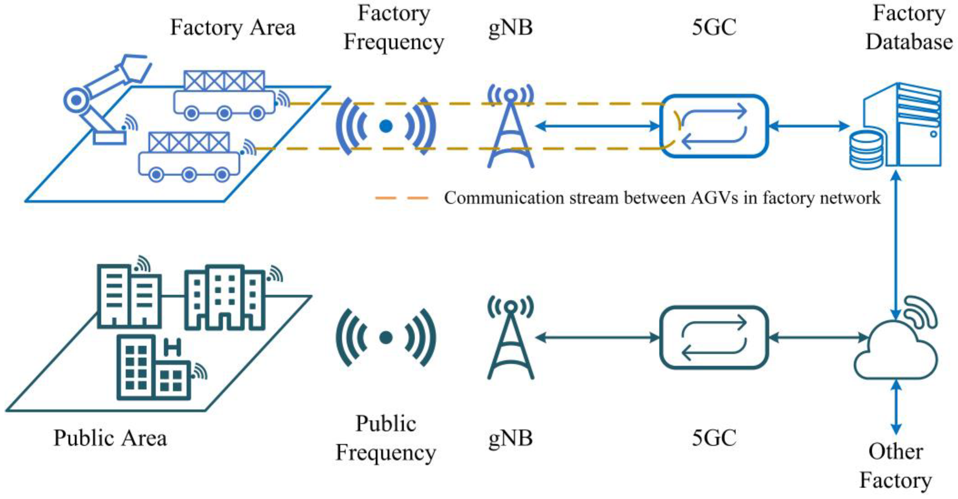
2.1. 5G Private Network Structure

For 5G network, factory automation scenarios have higher requirements than public scenarios on coverage, communication quality, latency, bandwidth, data confidentiality, device mobility, and network control authority. Therefore, private 5G networks are deployed to offer dedicated coverage, exclusive capacity, intrinsic control, customized service, and dependable communication [23]. The private network architecture can be divided into the following three types [24]: hybrid private networks, virtual private networks, and physical networks. In hybrid private networks and virtual private networks, industry will share or partly share the wireless equipment next Generation NodeB (gNB), 5G frequency, and 5G core network (5GC) with public. In physical private networks, industry users will have exclusive gNB, 5G frequency, and 5GC. Therefore, the physical private network is completely isolated from the public network. Network traffic and congestion in public network will not impact the quality of private network. The physical private network is oriented to industry applications that require extremely high reliability and privacy. This paper researched 5G characteristics in physical private network.

The structure of physical private network is shown in Figure 1. This paper is concerned with the communication process between the two AGVs. The end to end (E2E) delay in this paper refers to the time that it takes for the data packet to go through the AGV1-gNB-5GC-gNB- AGV2 equipment in the factory private 5G networks.

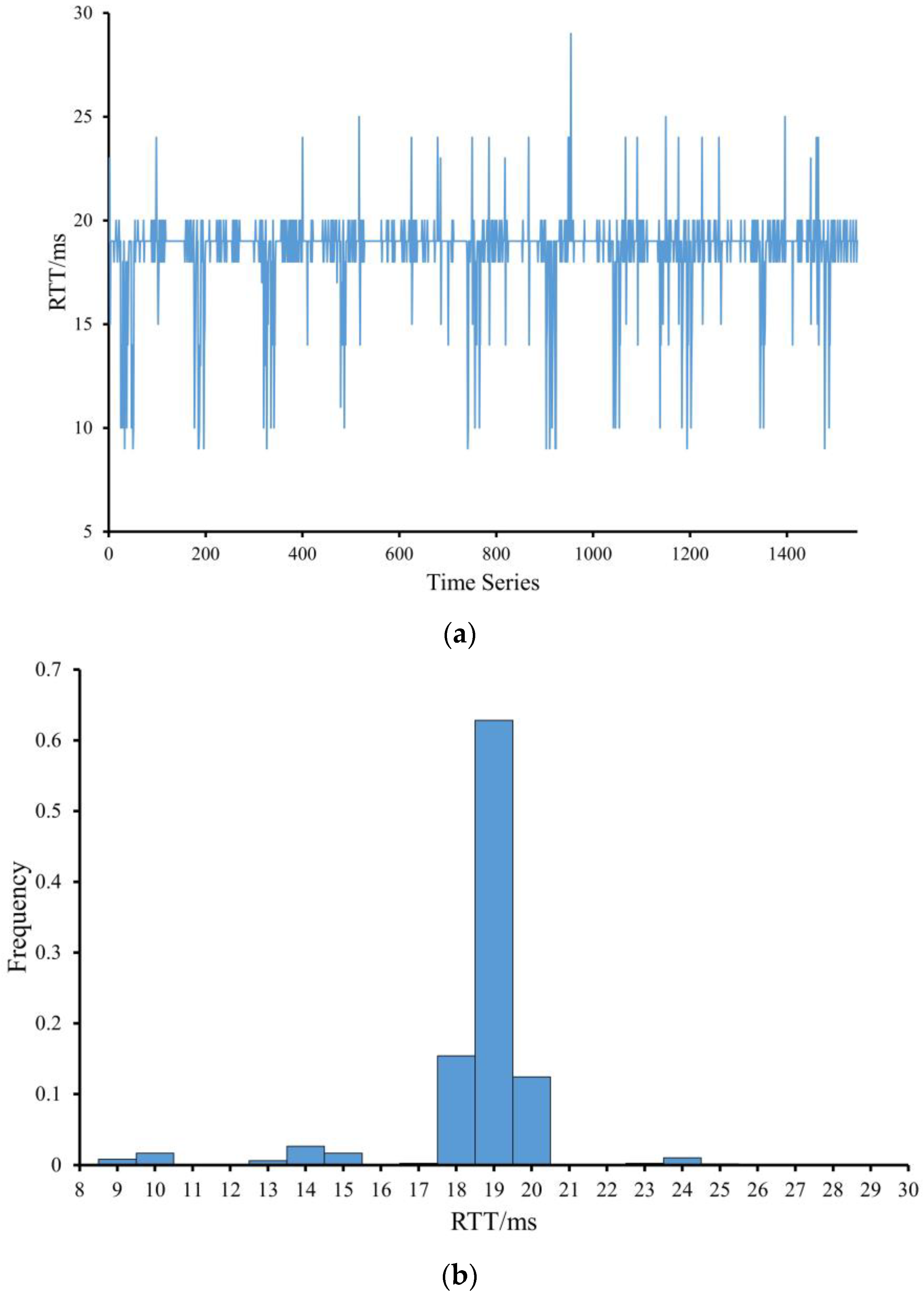
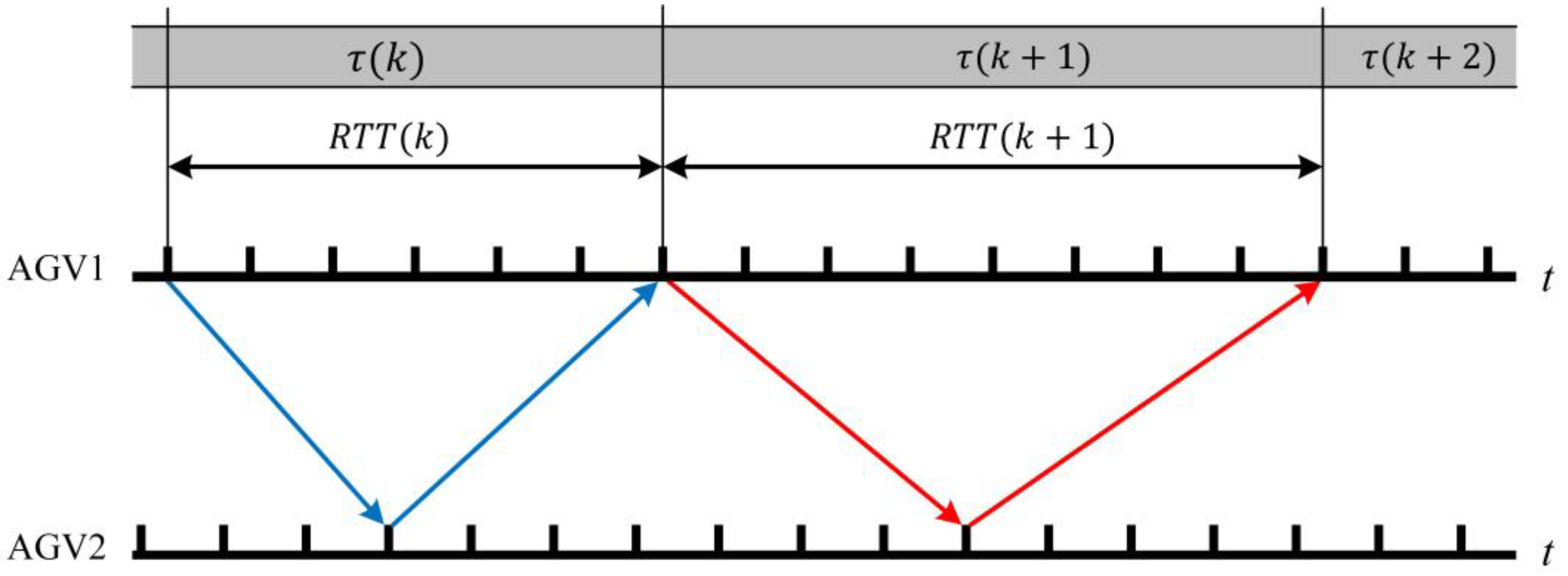
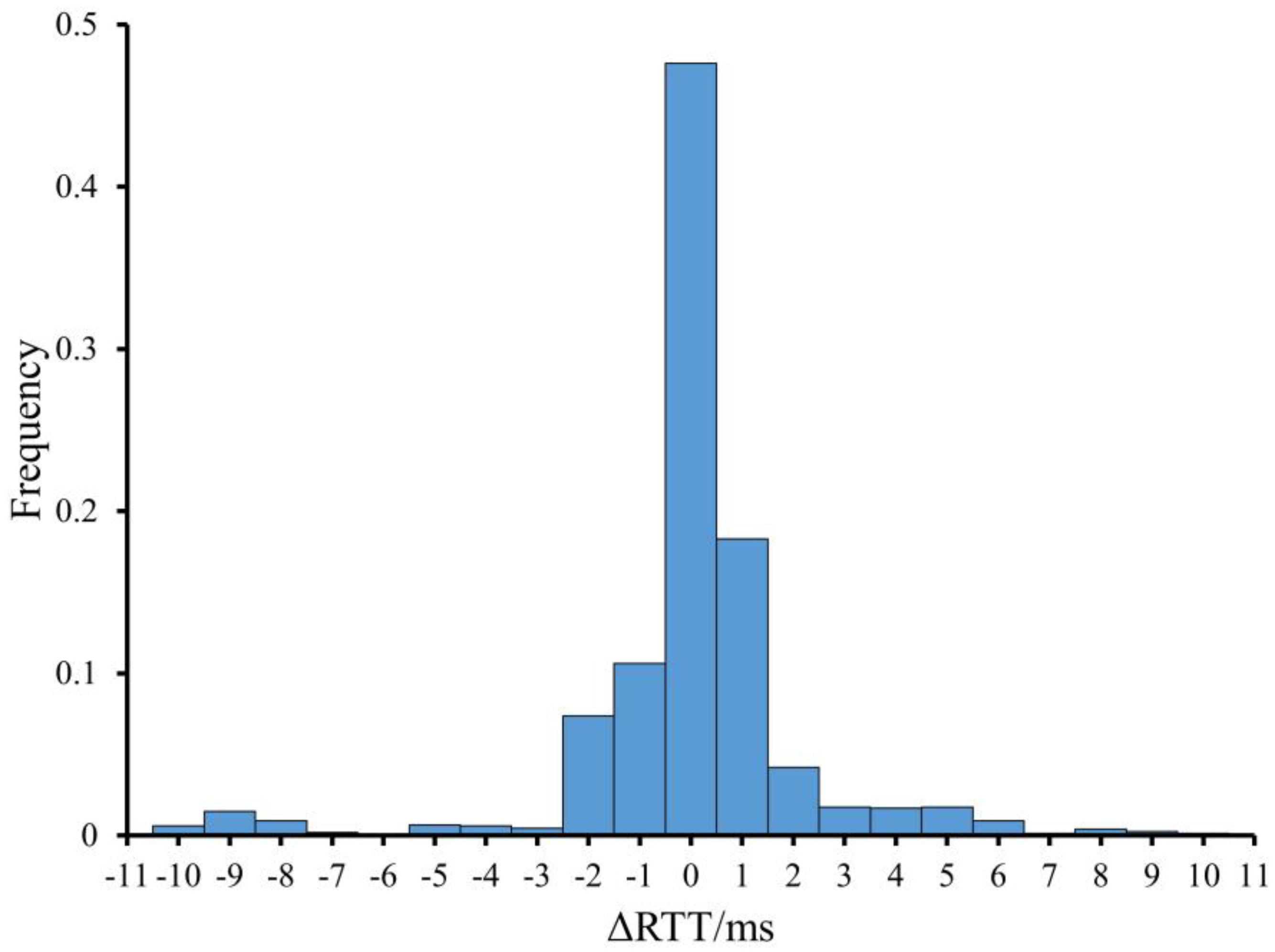
2.2. 5G Networks Delay Measurement and Analysis

The time delay is one of the most important factors that determines the efficiency of the NCS. Affected by time delay, the control command sent by the controller cannot take effect in time, and the controller cannot get accurate feedback. Before designing the control system in 5G networks, it is necessary to measure delay and analysis characteristics. To obtain the characteristic of 5G networks delay, some researchers have made effort on measurement and analysis of the 5G networks delay [25,26]. They both used clock-synchronized devices to measure air interface delay or E2E delay in laboratory conditions. However, it is difficult to synchronize the clocks of 2 AGV through wireless networks in factory. E2E delay cannot be measured directly without clock synchronization. Therefore, Round Trip Time (RTT) is used to characterize the delay. In this paper, RTT refers to the time it takes for AGV1 from send information to AGV2 and receive the reply. For measuring the RTT, one controller sends the data packet to another and records the sending time and receiving reply time by system clock. RTT is the difference between sending time and receiving time.

The measurements are carried out in a physical private network in factory. The network parameters are shown in

Table 1. Parameters of 5G networks.

Parameters	Value
Frequency	2.6 GHz
Bandwidth	100 MB
Signal to Noise Ratio	20 dB
Reference Signal Receiving Power	−85 dBm

. The 2 AGV are in the same room and the distance between 2 AGVs is 1200 mm. The 5G Customer Premise Equipment (5G CPE) is a product of Lierda MX880 while the RTT is calculated by Beckhoff embedded PC CX5010 with Intel Atom Z510 processor, 512 MB RAM, and a Windows Embedded CE 6 operating system. The 5G CPE is connected to CX5010 through the EtherCAT EAP protocol.

This paper constantly measured 1546 sets of RTT in 30 s and the results are shown in Figure 2. Define

$$\Delta RTT\left(k\right)=RTT\left(k\right)-RTT\left(k-1\right)$$

(1)

Histogram of ΔRTT is shown in Figure 3.

Figure 2 shows that the RTT of the 5G network has randomness and multi-peak characteristics. The peak-to-peak intervals are approximately 5 ms. RTT is mainly concentrated around 19 ms (17–22 ms, 90.89%). The RTT measured consists of the terminal processing delay, core network processing delay, and air interface delay. There are some factors such as time-division duplex (TDD) uplink-downlink conversion cycle and retransmission which could cause the multi-feature feature. The TDD uplink-downlink conversion usually causes jitters in 0–5 ms and retransmission in MAC layer also bring jitters in 5–20 ms.

Figure 3 shows the distribution of ΔRTT to reflect the delay changes. A total 88.1% of the data are in 0 ± 2 ms and 90.3% in 0 ± 3 ms. There are still some large jitters but it occurs less frequently. With the development of 5G, network technologies such as network slicing and resource scheduling can further improve network quality and reduce jitter [7].

In summary, the RTT of 5G transmission has randomness, but most of them are still concentrated in 19 ± 3 ms. The jitter of RTT is relatively gentle and mainly concentrated in 0 ± 3 ms.

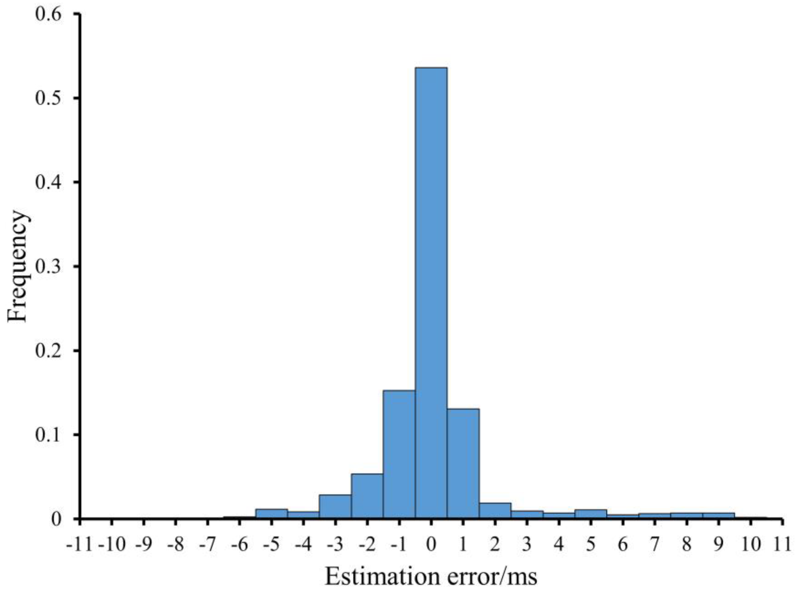
2.3. 5G Delay Estimation

While AGV1 measures RTT, AGV2 will actively send data to AGV1 in collaborative transport. AGV1 could not obtain the delay of current data of AGV2. In the situation, the following work is to estimate the delay of current transmission by using previous RTT. Researchers have proposed many estimation methods, including neural network methods [27], time series analysis methods [28] and Kalman filter methods [19]. Both neural network method and time series analysis method will bring large computing load to controller, which may affect the accuracy of servo control. In contrast, Kalman filter method requests less computing resource and is suitable for real-time control.

As a typical real-time control system, AGV system sets most closed-loop control in local to ensure the stability and accuracy, which requires an estimation method with less computation load. Therefore, Kalman filter method is applied to estimate delay in this paper.

This paper has the following assumptions in the estimation of delay:

(1)

In a round-trip transmission, the two E2E delay are equal.

(2)

The communication network is relatively stable between two RTT measurements.

If assumption 1 is established, RTT/2 can be used to express the E2E delay. If assumption 2 is established, the estimation of RTT can be used to represent the network status in the time between 2 round-trip time measurements. The conclusion in Section 2.2 shows that the RTT jitter is relatively stable. Meanwhile, it is a vital serious safety risk that network conditions violently and rapidly fluctuate. Devices will not continue to work in this situation. Therefore, it can be considered that assumption 2 is established.

Considering the conclusions of Section 2.2 and referring to the [19], the delay of the transmission process could be modeled as

$$\left\{\begin{array}{c}\tau \left(k+1\right)=\tau \left(k\right)+a\left(k\right)\\ y_{rrt}\left(k\right)=\tau \left(k\right)+b\left(k\right)\end{array}\right.$$

(2)

where τ(k) refers to the current real RTT delay, a(k) is a white noise with a mean value of 0 and a covariance of Q. y_rrt(k) is the current measured RTT, and b(k) is a mean value of 0 white noise with covariance R.

Through the above modeling, the Kalman filter can be used to estimate the time delay. The formula for using the Kalman filter to estimate is

$$\left\{\begin{array}{cc}\hfill \tau \left(k\right)& =\tau \left(k-1\right)\hfill \\ \hfill P^{-}\left(k\right)& =P\left(k-1\right)+Q\hfill \\ \hfill K\left(k\right)& =\frac{P^{-}\left(k\right)}{P^{-}\left(k\right)+R}\hfill \\ \hfill \tau \left(k\right)& ={\tau }^{-}\left(k\right)+K\left(k\right)\left(y_{rrt}\left(k\right)-{\tau }^{-}\left(k\right)\right)\hfill \\ \hfill P\left(k\right)& =P^{-}\left(k\right)\left(1-K\left(k\right)\right)\hfill \end{array}\right.$$

(3)

To better reflect the influence of the current data in the long-time operation, the forgetting factor λ is often deployed. Thus it can be rewritten as

$$K\left(k\right)=\frac{1}{\lambda }\frac{P^{-}\left(k\right)}{P^{-}\left(k\right)+R}$$

(4)

The process of obtaining the estimated value of time delay is shown in Figure 4. AGV 1 will continue to measure RTT and generate an estimate delay τ(k) once RTT(k − 1) is obtained. Before RTT(k) is obtained, the τ(k) will represent the network delay status.

There are some statistical estimation methods [29] such as the mean method (5), median method (6), and max value method (7).

$$\tau \left(k+1\right)=\mathrm{mean}\left\{RTT\left(k\right),RTT\left(k-1\right),\dots ,RTT\left(1\right)\right\}$$

(5)

$$\tau \left(k+1\right)=\mathrm{median}\left\{RTT\left(k\right),RTT\left(k-1\right),\dots ,RTT\left(1\right)\right\}$$

(6)

$$\begin{array}{c}\tau \left(k+1\right)=\max \left\{\mathrm{mean}\left(RTT\left(k\right),RTT\left(k-1\right),\dots ,RTT\left(1\right)\right),\right.\\ \left.\mathrm{median}\left(RTT\left(k\right),RTT\left(k-1\right),\dots ,RTT\left(1\right)\right)\right\}\end{array}$$

(7)

The τ(k) is estimated from RTT(k − 1). The RTT data measured in Section 2.2 is used to verify the performance of the Kalman filter estimate method with Q = 0.4, R = 16 λ = 1. Using root mean square error (RMSE)

$$S_e=\sqrt{\frac{{{\displaystyle \sum }}_{k=1}^{k=n}{\left(RTT\left(k\right)-\tau \left(k\right)\right)}^2}{n}}$$

(8)

to characterize the performance of estimation methods.

Table 2. RMSE of methods.

Method	Se/ms
Kalman Filter	1.8916
Mean	2.0482
Median	2.0329
Max value	2.0914

shows the $S_e$ of Kalman filter method and the above statistical methods. The result shows the Kalman Filter method has better performance than mean method, median method, and max value method. Figure 5 shows the estimation error histogram of Kalman Filter method. A total 91.66% of the estimation errors are in 0 ± 3 ms. There are still some large errors but this occurs less frequently and could be ignored. According to the above assumptions, the E2E delay of the two AGVs can be expressed as τ/2. Therefore, the upper and lower bounds of the error will be smaller.

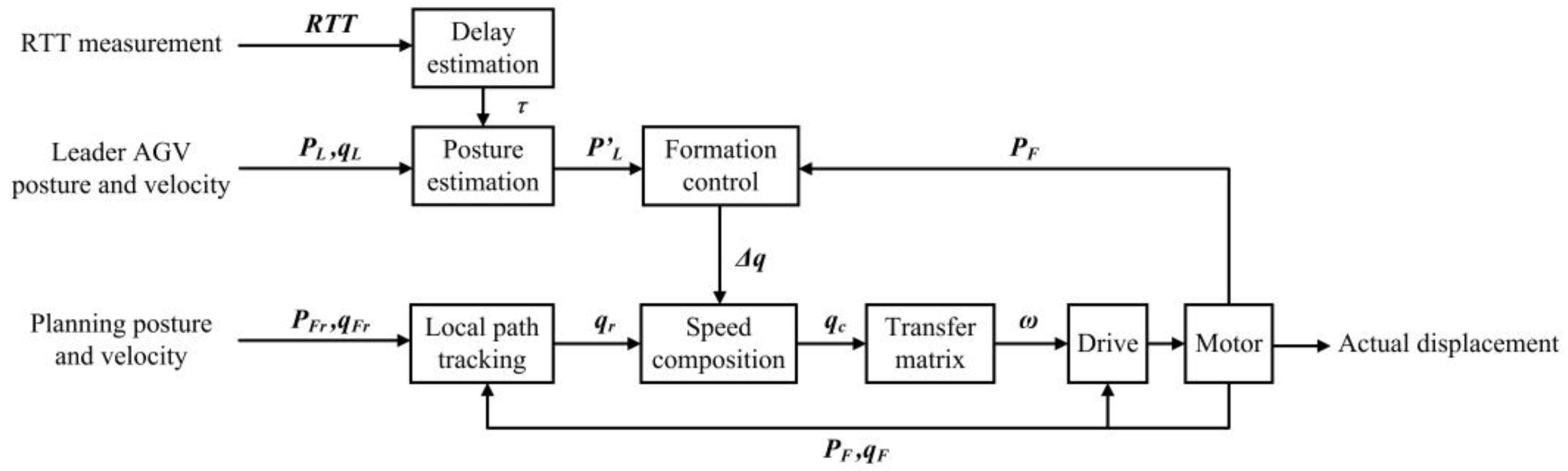
3. Formation Control System Design

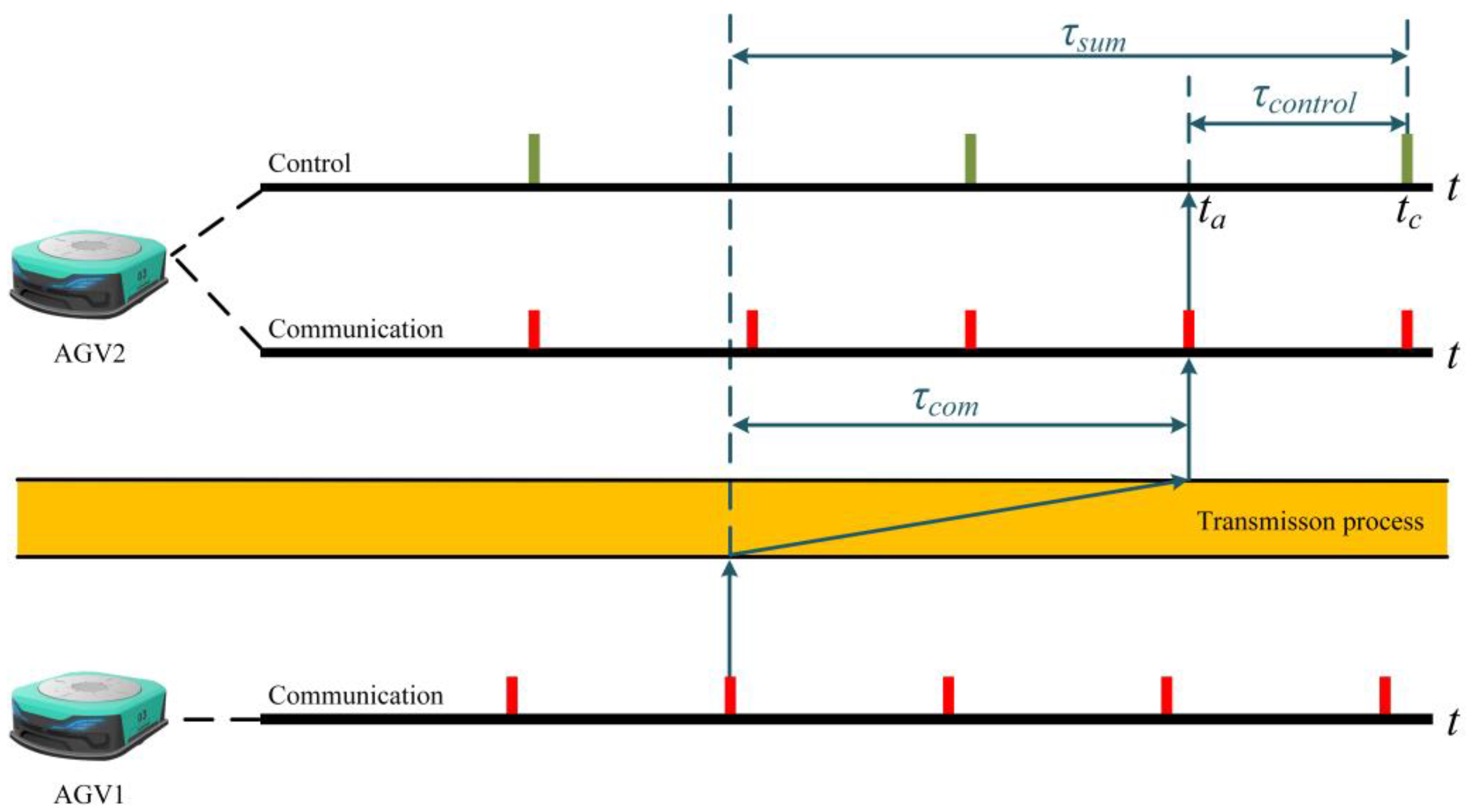
3.1. Delay Analysis in Control System

Section 2 analyzed the 5G transmission delay and proposed an estimation method for communication delay. In NCS, the relationship between the communication cycle T_com and the control cycle T_control may also cause delay. Effective control commands require new data. Therefore, T_control < T_com will not be considered. When network conditions are stable, T_control = T_com is the optimal setting. However, 5G communication has randomness and there may be no new data in one communication period. To ensure that new data can be obtained in each control cycle, this paper sets T_control > T_com.

Therefore, the 5G NCS total delay τ_sum of data from generation to validation consists of the following two parts:

(1)

Network transmission delay τ_com: This delay describes the time that takes for data packet to AGV2 application layer from AGV1 application layer, which is the E2E delay mentioned above.

(2)

Execution waiting delay τ_control: This delay describes the time that takes for data packet from being received to being processed.

Therefore, τ_sum = τ_com + τ_control. Figure 6 shows a schematic diagram of the τ_sum in the case of T_com < T_control.

τ_control can be calculated by the system clock at the receiving end. The receiving end usually sets the data packet buffer to deal with the out-of-order. Therefore, the receiving end processing flow is as follows:

Step1: Obtain the decoded data of 5G CPE, record the current time as the arrival time t_a of the data packet, and store the date packet sequence number, content and t_a in the variable of controller.

Step2: Compare the packet sequence number with the data in the buffer, and the buffer retains the data packet with latest sequence number.

Step3: When the formation control is processing, the difference between the current system time t_c and the buffer data t_a can be used to obtain τ_control, which can be combined with the delay predicted in Section 2 to obtain the total data delay τ_sum = τ_com + τ_control = t_c − t_a + τ/2.

3.2. Discussion on Control Method Considering 5G Delay

The time delay caused by the 5G transmission and control cycle has been analyzed in Section 3.1. These delays cannot be ignored in real-time systems, and control method needs to be considered to reduce the impact of delays on the system. There are two main directions to reduce the impact of delay on the control system. One is to modify the network configurations to reduce the delay as much as possible. The other is to design a control method that considers the delay. This paper uses compensation control method to design the control system considering 5G delay.

The idea of the compensation control method is to estimate the current state of the system by using the delay value and the state model, and then compensate the control signal to reduce the influence of delay on the control system. Most industrial motion equipment has a relatively complete motion state model, which makes it possible to estimate its posture. Meanwhile, for different control objects, the compensation method can be quickly transplanted. Delay estimation is a common algorithm for all equipment. For each equipment, it only needs to replace the state model according to its own.

The scenario studied in this paper is of two AGVs in collaborative transport. It is necessary to ensure that the AGVs in the transport processing could maintain a stable formation. The leader-follower method is widely used due to its high reliability. The idea of the leader-follower method is to designate one AGV as the leader and the other AGVs as followers. The followers keep the distance and angle from the leader. In this paper, the leader AGV sends its posture to the follower and the follower regulates its motion state according to its own posture and the posture of the leader after receiving. To ensure that single AGV can operate stability in poor network conditions, the path tracking control still operates in local. The formation control will offer additional velocity command to regulate the corresponding posture to leader AGV. The actual planning velocity will be a composition of path tracking velocity and formation velocity. Therefore, the content of compensation is that the follower uses the time delay value obtained in Section 3.1 and the motion model of the AGV to obtain the current posture of the leader AGV then obtain the formation control signal.

Figure 7 shows the control system structure of follower AGV. RTT is the round-trip time measured by follower AGV and τ is the estimated E2E delay of the data from leader AGV. P_L, q_L are the posture and velocity of leader AGV in data packet, and P′_L is the estimated posture of leader AGV in current time. P_Fr, q_Fr are the planning posture and velocity of follower AGV. q_r is the path tracking velocity of follower AGV, and Δq is the additional formation velocity of follower AGV. q_c is the actual command velocity composed by q_r and Δq. ω is the actual command angle velocity of drive wheels.P_F, q_F are the posture and velocity of follower AGV.

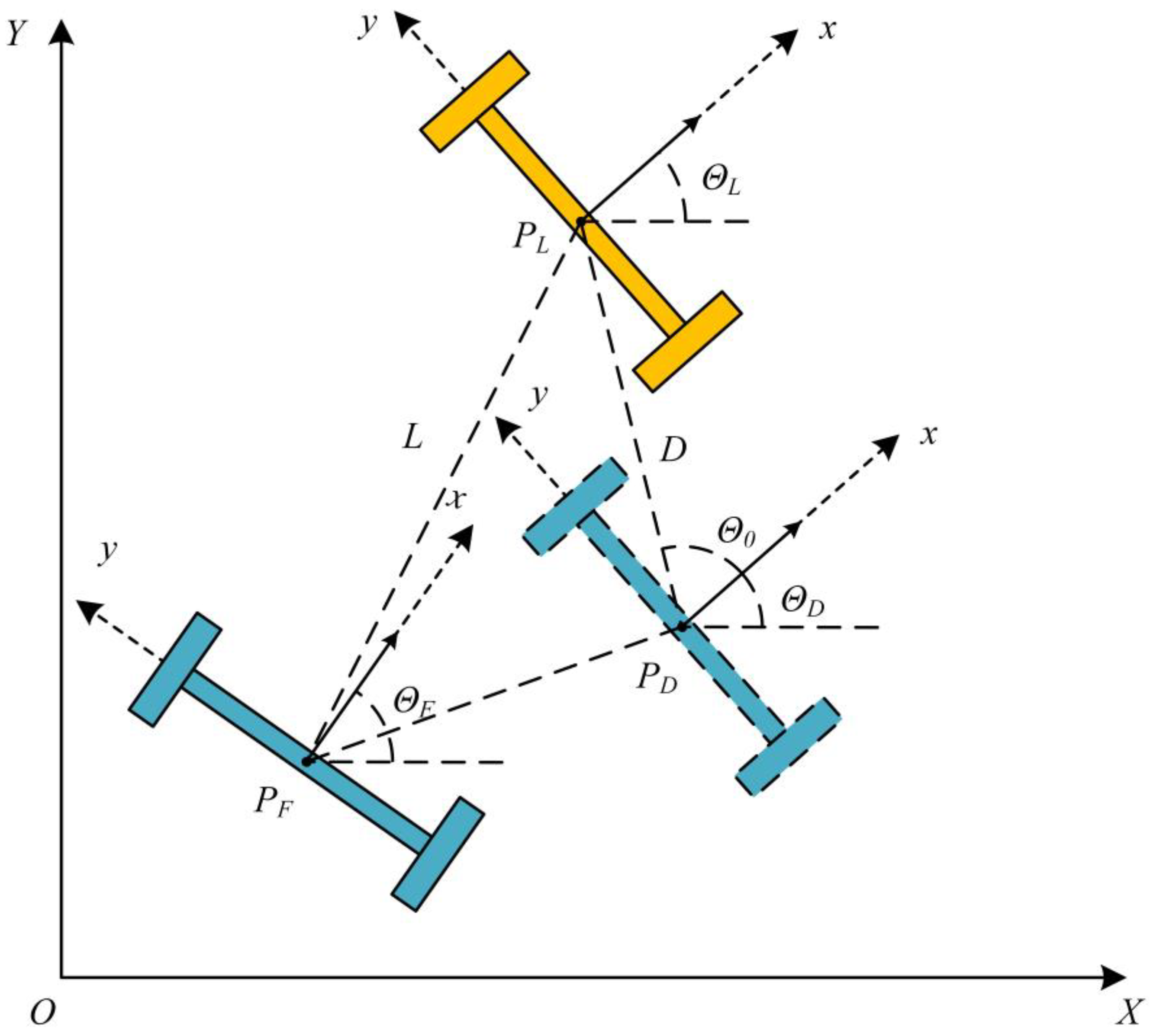
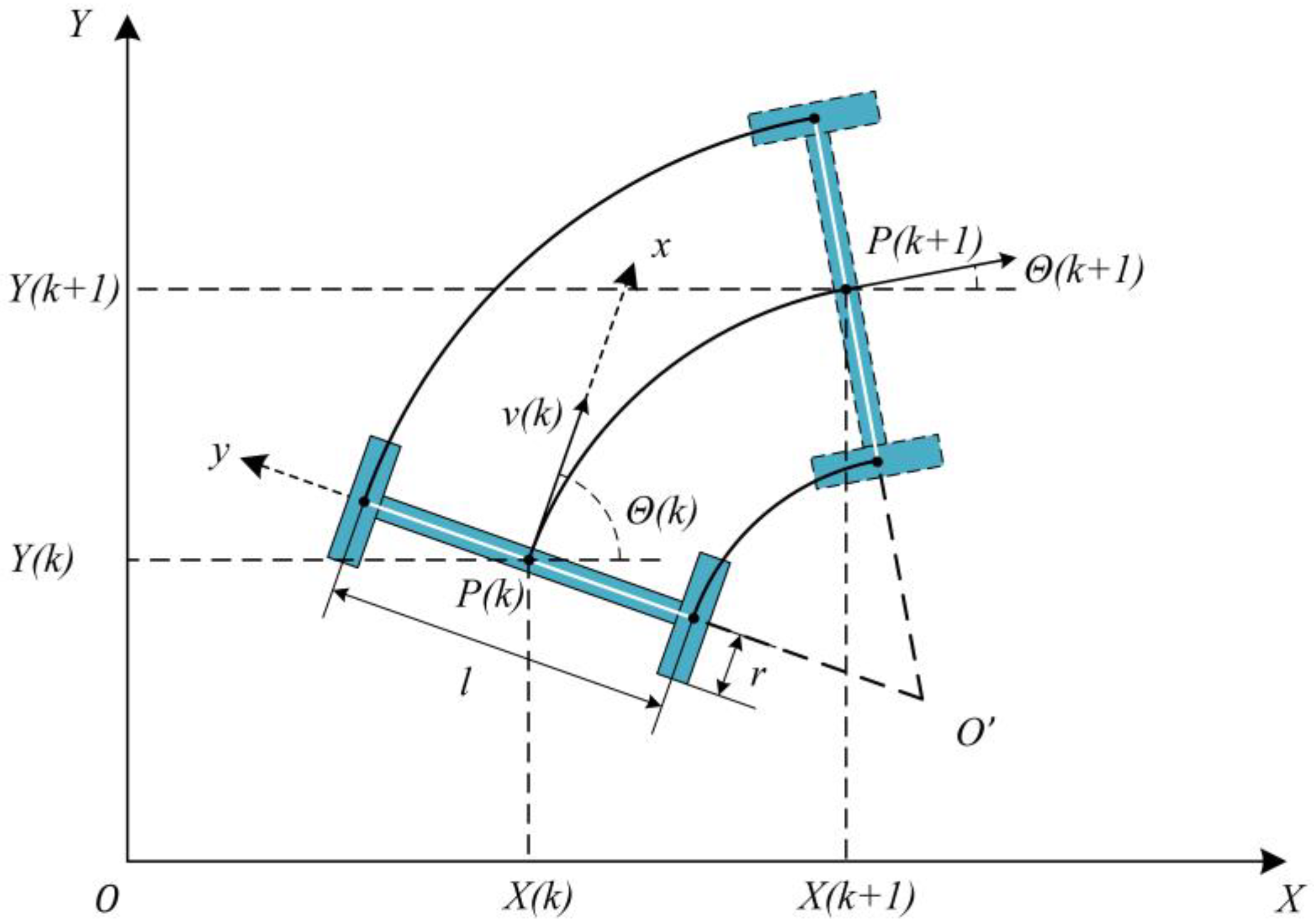
3.3. AGV Kinematic Model and Posture Estimation

Section 3.1 describes the total delay in control systems. The following work uses total delay and AGV motion model to estimate the posture of leader AGV.

Figure 8 shows the kinematics model of two-wheel differentially driven AGV. P (X, Y, Θ) and p (x, y, θ) represent the posture of AGV in global XOY coordinates and co-moving xoy coordinates. The origin of xoy is at the center of the two differential wheels and the x-axis points to the forward direction of the AGV. The transfer matrix from global frame to co-moving frame is

$$\mathit{T}=\left[\begin{array}{ccc}\cos \Theta & \sin \Theta & 0\\ -\sin \Theta & \cos \Theta & 0\\ 0& 0& 1\end{array}\right]$$

(9)

Let the radius of two driving wheels be r and the distance be l, and the angular velocity of the left and right wheels could be represented by ω_l ω_r, then [30]

$$\dot{\mathit{P}}=\left[\begin{array}{c}\dot{X}\\ \dot{Y}\\ \dot{\Theta }\end{array}\right]=\left[\begin{array}{cc}\frac{r}{2}\cos \Theta & \frac{r}{2}\cos \Theta \\ \frac{r}{2}\sin \Theta & \frac{r}{2}\sin \Theta \\ -\frac{r}{l}& \frac{r}{l}\end{array}\right]\left[\begin{array}{c}{\omega }_l\\ {\omega }_r\end{array}\right]=\left[\begin{array}{cc}\cos \Theta & 0\\ \sin \Theta & 0\\ 0& 1\end{array}\right]\left[\begin{array}{c}v\\ \omega \end{array}\right]=\mathit{J}\mathit{q}$$

(10)

where v is the AGV linear velocity, ω is the AGV rotational velocity, q is the AGV velocity vector in the co-moving coordinate, and J is a Jacobian matrix.

Assuming the angular velocities of the two wheels do not change in the time Δt and the posture P(k) = [X(k) Y(k) Θ(k)]^T, then there is

$$\mathit{P}\left(k+\mathsf{\Delta }t\right)=\left[\begin{array}{c}X\left(k\right)+v\left(k\right)\mathsf{\Delta }t\cos \left(\Theta \left(k\right)+\frac{\mathsf{\Delta }t}{2}\omega \left(k\right)\right)\\ Y\left(k\right)+v\left(k\right)\mathsf{\Delta }t\sin \left(\Theta \left(k\right)+\frac{\mathsf{\Delta }t}{2}\omega \left(k\right)\right)\\ \Theta \left(k\right)+\omega \left(k\right)\mathsf{\Delta }t\end{array}\right]$$

(11)

Therefore, the leader AGV sends its posture P and velocity q to the follower AGV. Follower AGV could use the P, q and τ_sum to estimate the posture of leader AGV in current time.

3.4. Formation Control and Speed Composition

As shown in Figure 9, P_L, P_F and P_D are the actual position of the leader AGV, the actual position of the follower AGV, and the expected position of the follower AGV. L is the actual distance between the leader AGV and the follower AGV, D is the expected distance between the leader AGV and the follower AGV, Θ_L, Θ_F, Θ_D are the actual angle of the leader AGV, the actual angle of follower AGV, and the expected angle of the follower AGV. In this paper, we set Θ_L = Θ_D. Θ₀ is the formation angle of follower AGV. Θ₀ and D determine the follower AGV’s posture relative to the leader AGV. Θ₀ and D will be chosen at the start of formation motion and known to leader AGV and follower AGV. In this paper, we focus on the distance error error_d and angle error error_a. There is

$$\left\{\begin{array}{cc}\hfill erro{r}_d\left(k\right)& =\left|D-L\left(k\right)\right|\hfill \\ \hfill erro{r}_a\left(k\right)& =\left|{\Theta }_d\left(k\right)-{\Theta }_L\left(k\right)\right|\hfill \end{array}\right.$$

(12)

According to the geometric relationship, there is

$$\left\{\begin{array}{cc}\hfill X_D& =X_L-D\cos \left({\Theta }_L+{\Theta }_0\right)\hfill \\ \hfill Y_D& =Y_L-D\sin \left({\Theta }_L+{\Theta }_0\right)\hfill \\ \hfill {\Theta }_D& ={\Theta }_L\hfill \end{array}\right.$$

(13)

Then the deviation of P_D relative to P_F is

$$\left\{\begin{array}{cc}\hfill e_X& =X_L-D\cos \left({\Theta }_L+{\Theta }_0\right)-X_F\hfill \\ \hfill e_Y& =Y_L-D\sin \left({\Theta }_L+{\Theta }_0\right)-Y_F\hfill \\ \hfill e_{\Theta }& ={\Theta }_L-{\Theta }_F\hfill \end{array}\right.$$

(14)

With the transfer matrix T (9), the error can be represented in co-moving coordinates as

$$\left[\begin{array}{c}{e}_x\\ e_y\\ e_{\theta }\end{array}\right]=\left[\begin{array}{ccc}\cos {\Theta }_F& \sin {\Theta }_F& 0\\ -\sin {\Theta }_F& \cos {\Theta }_F& 0\\ 0& 0& 1\end{array}\right]\left[\begin{array}{c}{e}_X\\ e_Y\\ e_{\Theta }\end{array}\right]$$

(15)

[e_x e_y e_θ] ^T is the input of formation control, and a proportional control is used to obtain the additional velocity. There is

$$\left\{\begin{array}{c}\Delta v_{xf}=k_1{e}_x\\ \Delta v_{yf}=k_2{e}_y\\ \Delta {\omega }_f=k_3{e}_{\theta }\end{array}\right.$$

(16)

The formation additional velocity is ΔV = [Δvxf Δvyf Δωf]^T, ΔV could be transferred to Δq = [Δv Δω]^T according to control system and matrix. The path tracking velocity is q_r and the actual command velocity is q_c = q_r + Δq, qc can be transferred to the actual angle velocity ω = [ω_l ω_r]^T of two driving wheels.

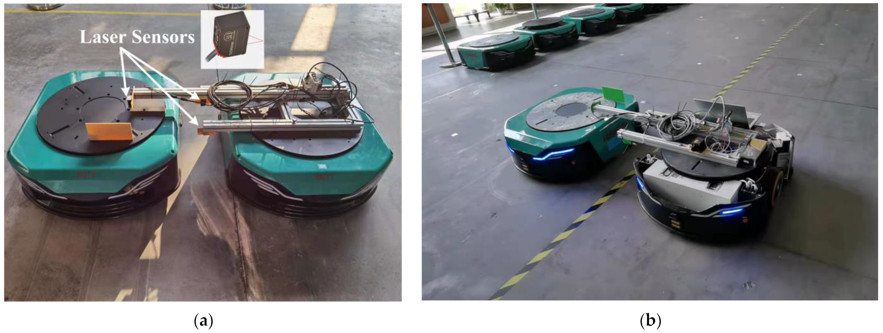
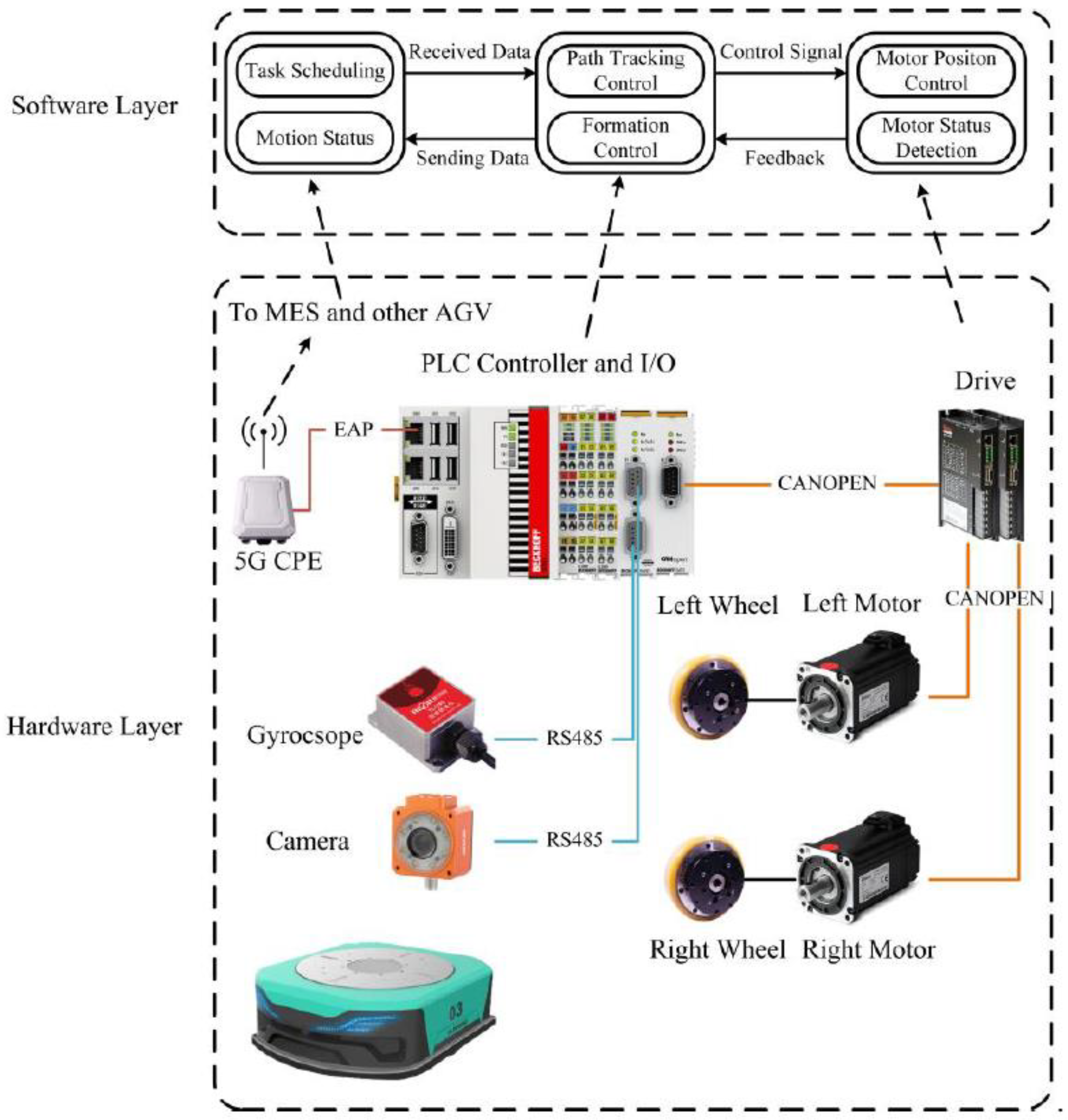
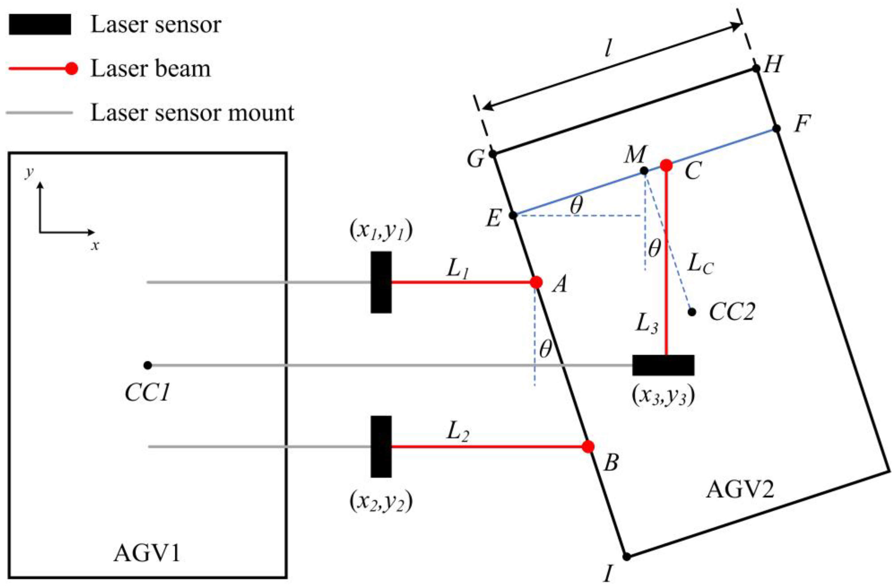
4. Experiment and Result

The AGV in this paper is product of Huaheng welding company, type of Muliuliuma-500. The parameters of the AGV used in this paper are shown in

Table 3. Parameters of AGV.

Parameter	Value	Unit
Size	1000 × 805 × 300	mm
Weight	210	kg
Maximum load	500	kg
Radius of driving wheel	105	mm
Distance between driving wheel	718	mm
Maximum accelerates	0.6	m/s2
Guided method	QR	-
Drive method	Different drive	-

.

The control system is developed by TwinCAT2 and the controller is Beckhoff CX5010. The 5G CPE is the product of Lierda. The 5G CPE is connected to the controller through the EtherCAT EAP protocol and the communication protocol of the servo motor is CANOPEN.

The architecture of the AGV system is shown in the Figure 10.

Three optoNCDT 1420 laser sensor of Micro-Epsilon are used to measure the distance, the difference of two AGV postures [Δx Δy Δθ] ^T could be obtained by calculation.

Figure 11 shows the measurement method of posture error δ with 3 laser sensors.CC1 and CC2 are the geometric centers of 2 AGVs. The coordinate is set as Figure 11 and CC1 is the origin. (x₁, y₁), (x₂, y₂) and (x₃, y₃) are the three sensor positions while L₁, L₂ and L₃ are distance measured by 3 sensors. A (x_a, y_a), B (x_b, y_b) and C (x_c, y_c) are the laser beam measurement points on the AGV2. GH and GI are the edges of AGV 2 and GH is vertical to GI. A reflector is installed parallel to GH on AGV2. The distance between the reflector and CC2 is L_C. EF is the line where the reflector is located. C is on the EF and M is the midpoint of the EF. By calculating the position of CC2, the δ could be obtained.

This paper has two assumptions:

(1)

The measurement equipment is installed accurately to ensure $\overrightarrow{L_1}, \overrightarrow{L_2}$ ⫽ $\overrightarrow{x}$, $\overrightarrow{L_3}$ ⫽ $\overrightarrow{y}$, EF ⫽ GH. Therefore, |EF| = l and |DCC2| = L_C.

(2)

There is no deformation on both AGV’s body and measurement equipment during measurement operation.

The laser beam measurement positions are A (x_a, y_a) = (x₁ + L₁, y₁), B (x_b, y_b) = (x₂ + L₂, y₂), and C (x_c, y_c) = (x₃, y₃ + L₃). A and B are both on the edge of AGV2, so the difference of heading direction angle is

$$\theta =\arctan \frac{L_2-L_1}{y_1-y_2}$$

(17)

The slope and equation of AB are

$$\left\{\begin{array}{c}{K}_{AB}=\frac{y_b-y_a}{x_b-x_a}\\ L_{AB}:y-y_a=K_{AB}\left(x-x_a\right)\end{array}\right.$$

(18)

Geometric relationship shows AB ⊥ EF and C is on the EF. The slope and equation of EF are

$$\left\{\begin{array}{c}{K}_{EF}=-\frac{1}{K_{AB}}=-\frac{x_b-x_a}{y_b-y_a}\\ L_{AB}:y-y_c=K_{EF}\left(x-x_c\right)\end{array}\right.$$

(19)

As the intersection of AB and EF, the position of E (x_e, y_e) could be calculated by (18) and (19). There is

$$\left\{\begin{array}{c}{x}_e=\frac{K_{AB}{x}_a-K_{EF}{x}_c+y_c-y_a}{K_{AB}-K_{EF}}\\ y_e=K_{AB}\left(x_e-x_a\right)+y_a\end{array}\right.$$

(20)

Then midpoint M is applied to calculate the position of CC2. According to the geometric relationship, there is

$$\left\{\begin{array}{c}{x}_{C{C}_2}=x_e+l\cos \theta +L_c\sin \theta \\ y_{C{C}_2}=y_e+l\sin \theta -L_c\cos \theta \end{array}\right.$$

(21)

The posture difference δ = [Δx Δy Δθ] ^T = [ x_CC2 y_CC2 θ] ^T.

The dual-AGV collaborative transport experiment systems and environment are shown in Figure 12.

In this experiment, the two AGVs are set to move 7200 mm along a straight line, and the speed is set to 0.8 m/s. The formation angle Θ₀ is 90° and expected distance D is 1200 mm. Network parameters are shown in Table 1. In the formation algorithm, k₁ = 0.1, k₂ = 0.1, k₃ = 0.01, and the formation control cycle is 16 ms.

To eliminate the influence of network conditions, we repeated the experiment three times. As comparison, we tested the formation motion accuracy without formation control in the same kinematic parameters. The results of the experiments are shown in Figure 13.

5. Conclusions

Focusing on the collaborative transport of dual AGVs, this paper researched the formation control based on compensation method in 5G R15 network. Firstly, the RTT is measured and analyzed in physical private network. The result shows that the distribution of RTT is random and RTT is mainly concentrated in 19 ± 3 ms. The jitter of RTT is mainly distributed in 0 ± 3 ms. Kalman filter method is applied to estimate the RTT, and the result shows the effectiveness of Kalman filter method. The total delay in control system has been discussed considering the communication delay and executing delay. AGV kinematic model has been established and used to estimate the current position of leader AGV considering total delay. Formation model and control method have been established to regulate the motion status of follower AGV to maintain the formation accuracy. Finally, an experiment was carried out. The experiment results show that the control method and process proposed in this paper can effectively improve the accuracy of AGV formation motion.

This paper does not consider the influence of wheel slip, load change etc. A more complete dynamic model can ensure the posture estimation accuracy in the above situations. Moreover, the effectiveness of the control system in different network loads has not been further analyzed. The further work will focus on the two estimations proposed in the article. The first will be how to use the data to get the better estimation of the current network delay in different network loads, and the second will be how to better estimate the relative posture of the leader AGV considering dynamic model.

References

1. Rodriguez, I.; Mogensen, R.S.; Schjorring, A.; Razzaghpour, M.; Maldonado, R.; Berardinelli, G.; Adeogun, R.; Christensen, P.H.; Mogensen, P.; Madsen, O.; et al. 5G Swarm Production: Advanced Industrial Manufacturing Concepts Enabled by Wireless Automation. IEEE Commun. Mag. 2021, 59, 48–54. [Google Scholar] [CrossRef]
2. 5G Use Cases for Verticals China 2020. Available online: https://www.gsma.com/greater-china/resources/5g-use-cases-for-verticals-china-2020-3/ (accessed on 1 September 2021).
3. Report on Implementation of Options for Monitoring of Workpiece and Machines. Available online: https://5gsmart.eu/wp-content/uploads/5G-SMART-D3.3-v1.0.pdf (accessed on 15 September 2021).
4. Release 16 Description; Summary of Rel-16 Work Items. Available online: https://www.3gpp.org/ (accessed on 10 September 2021).
5. Ghosh, A.; Maeder, A.; Baker, M.; Chandramouli, D. 5G Evolution: A View on 5G Cellular Technology beyond 3GPP Release 15. IEEE Access 2019, 7, 127639–127651. [Google Scholar] [CrossRef]
6. Rodriguez, I.; Mogensen, R.S.; Fink, A.; Raunholt, T.; Markussen, S.; Christensen, P.H.; Berardinelli, G.; Mogensen, P.; Schou, C.; Madsen, O. An Experimental Framework for 5G Wireless System Integration into Industry 4.0 Applications. Energies 2021, 14, 4444. [Google Scholar] [CrossRef]
7. Rost, P.; Mannweiler, C.; Michalopoulos, D.S.; Sartori, C.; Sciancalepore, V.; Sastry, N.; Holland, O.; Tayade, S.; Han, B.; Bega, D.; et al. Network Slicing to Enable Scalability and Flexibility in 5G Mobile Networks. IEEE Commun. Mag. 2017, 55, 72–79. [Google Scholar] [CrossRef] [Green Version]
8. 5G Smart Project. Available online: https://5gsmart.eu/ (accessed on 15 September 2021).
9. Holfeld, B.; Wieruch, D.; Wirth, T.; Thiele, L.; Ashraf, S.A.; Huschke, J.; Aktas, I.; Ansari, J. Wireless Communication for Factory Automation: An opportunity for LTE and 5G systems. IEEE Commun. Mag. 2016, 54, 36–43. [Google Scholar] [CrossRef]
10. Industrial 5G for the Industry of Tomorrow. Available online: https://new.siemens.com/global/en/products/automation/industrial-communication/industrial-5g.html (accessed on 10 September 2021).
11. Koumaras, H.; Makropoulos, G.; Batistatos, M.; Kolometsos, S.; Gogos, A.; Xilouris, G.; Sarlas, A.; Kourtis, M.-A. 5G-Enabled UAVs with Command and Control Software Component at the Edge for Supporting Energy Efficient Opportunistic Networks. Energies 2021, 14, 1480. [Google Scholar] [CrossRef]
12. Montonen, J.; Koskinen, J.; Makela, J.; Ruponen, S.; Heikkila, T.; Hentula, M. Applying 5G and Edge Processing in Smart Manufacturing. In Proceedings of the 2021 IFIP Networking Conference (IFIP Networking), Espoo, Finland, 21–24 June 2021; pp. 1–2. [Google Scholar]
13. Ding, H.; Zhang, Y.; Xia, L.; Wang, Q. Use Cases and Practical System Design for URLLC from Operation Perspective. In Proceedings of the 2019 IEEE International Conference on Communications Workshops (ICC Workshops), Shanghai, China, 11 July 2019; pp. 1–6. [Google Scholar]
14. Oyekanlu, E.A.; Smith, A.C.; Thomas, W.P.; Mulroy, G.; Hitesh, D.; Ramsey, M.; Kuhn, D.J.; McGhinnis, J.D.; Buonavita, S.C.; Looper, N.A.; et al. A Review of Recent Advances in Automated Guided Vehicle Technologies: Integration Challenges and Research Areas for 5G-Based Smart Manufacturing Applications. IEEE Access 2020, 8, 202312–202353. [Google Scholar] [CrossRef]
15. Yoshioka, C.; Namerikawa, T. Formation Control of Nonholonomic Multi-Vehicle Systems based on Virtual Structure. IFAC Proc. Vol. 2008, 41, 5149–5154. [Google Scholar] [CrossRef] [Green Version]
16. Tlale, N.S. Fuzzy logic controller with slip detection behaviour for Mecanum-wheeled AGV. Robotica 2005, 23, 455–456. [Google Scholar] [CrossRef]
17. Consolini, L.; Morbidi, F.; Prattichizzo, D.; Tosques, M. Leader–follower formation control of nonholonomic mobile robots with input constraints. Automatica 2008, 44, 1343–1349. [Google Scholar] [CrossRef]
18. Wang, R.; Jing, H.; Hu, C.; Yan, F.; Chen, N. Robust H-infinity Path Following Control for Autonomous Ground Vehicles With Delay and Data Dropout. IEEE Trans. Intell. Transp. Syst. 2016, 17, 2042–2050. [Google Scholar] [CrossRef]
19. Lozoya, C.; Martí, P.; Velasco, M.; Fuertes, J.M.; Martín, E.X. Simulation study of a remote wireless path tracking control with delay estimation for an autonomous guided vehicle. Int. J. Adv. Manuf. Technol. 2010, 52, 751–761. [Google Scholar] [CrossRef]
20. Chen, Z.; Yang, J.; Zong, X. Leader-follower synchronization controller design for a network of boundary-controlled wave PDEs with structured time-varying perturbations and general disturbances. J. Frankl. Inst. 2021, 358, 834–855. [Google Scholar] [CrossRef]
21. Wang, J.Q.; Gao, J.F.; Zhang, X.J.; He, J.J. Formation Control of Time-varying Multi-agent System Based on BP Neural Network. In Proceedings of the 16th IEEE International Conference on Control, Automation, Robotics and Vision (ICARCV), Shenzhen, China, 13–15 December 2020; pp. 707–712. [Google Scholar]
22. Yang, Y.Q.; Jiang, H.J. Formation Control Based on Leader—Following Method for Multi—Robot to Reduce Path deviation. In Proceedings of the 29th Chinese Control and Decision Conference (CCDC), Chongqing, China, 28–30 May 2017; pp. 6607–6613. [Google Scholar]
23. Aijaz, A. Private 5G: The Future of Industrial Wireless. IEEE Ind. Electron. Mag. 2020, 14, 136–145. [Google Scholar] [CrossRef]
24. 5G Industry Application White Book. Available online: http://www.itei.cn/ewebeditor/uploadfile/20200914093949947.pdf (accessed on 10 September 2021).
25. Rischke, J.; Sossalla, P.; Itting, S.; Fitzek, F.H.P.; Reisslein, M. 5G Campus Networks: A First Measurement Study. IEEE Access 2021, 9, 121786–121803. [Google Scholar] [CrossRef]
26. Uitto, M.; Hoppari, M.; Heikkila, T.; Isto, P.; Anttonen, A.; Mammela, A. Remote Control Demonstrator Development in 5G Test Network. In Proceedings of the 2019 European Conference on Networks and Communications (EuCNC), Valencia, Spain, 15 August 2019; pp. 101–105. [Google Scholar]
27. Zhihao, G.; Malakooti, B. Delay Prediction for Intelligent Routing in Wireless Networks Using Neural Networks. In Proceedings of the 2006 IEEE International Conference on Networking, Sensing and Control, Ft. Lauderdale, FL, USA, 14 August 2006; pp. 625–630. [Google Scholar]
28. Guo, S.; Zhang, Y.; Zhu, S. Prediction of network signal transmission delay based on time aeries analysis. Railw. Comput. Appl. 2013, 22, 11–13. [Google Scholar] [CrossRef]
29. Zheng, L.; Vanijjirattikhan, R.; Chow, M.; Viniotis, Y. Comparison of real-time network traffic estimator models in gain scheduler middleware by unmanned ground vehicle network-based controller. In Proceedings of the Conference of IEEE Industrial Electronics Society, Raleigh, NC, USA, 16 January 2005. [Google Scholar]
30. Kanayama, Y.; Kimura, Y.; Miyazaki, F.; Noguchi, T. A stable tracking control method for an autonomous mobile robot. In Proceedings of the Proceedings., IEEE International Conference on Robotics and Automation, Cincinnati, OH, USA, 13–18 May 1990; pp. 384–389. [Google Scholar]
Figure 1. Structure of 5G physical private networks.
Machines 09 00318 g001
Figure 2. RTT measurement results (a) Timing diagram; (b) RTT distribution histogram.
Machines 09 00318 g002
Figure 3. ΔRTT distribution histogram.
Machines 09 00318 g003
Figure 4. Schematic diagram of Kalman filter delay estimation.
Machines 09 00318 g004
Figure 5. Estimation error distribution histogram.
Machines 09 00318 g005
Figure 6. Total delay in multi-cycle system.
Machines 09 00318 g006
Figure 7. Control system structure of follower AGV.
Machines 09 00318 g007
Figure 8. Schematic diagram of AGV kinematics.
Machines 09 00318 g008
Figure 9. Schematic diagram of leader-follower method.
Machines 09 00318 g009
Figure 10. Experiment AGV system architecture.
Machines 09 00318 g010
Figure 11. Measurement system schematic diagram.
Machines 09 00318 g011
Figure 12. Experiments systems: (a) AGVs with measurement systems; (b) Experiment operation.
Machines 09 00318 g012
Figure 13. Formation motion Error: (a) distance/mm; (b) angle/°.
Machines 09 00318 g013