Article

GPS Path Tracking Control of Military Unmanned Vehicle Based on Preview Variable Universe Fuzzy Sliding Mode Control

1
Automobile Engineering Research Institute, Jiangsu University, Zhenjiang 212013, China
2
Yangzhou Aoterui Automobile Electronic Technology Co., Ltd., Yangzhou 225008, China
*
Author to whom correspondence should be addressed.
Machines 2021, 9(12), 304; https://doi.org/10.3390/machines9120304
Submission received: 25 September 2021 / Revised: 7 November 2021 / Accepted: 12 November 2021 / Published: 23 November 2021
(This article belongs to the Topic Motion Planning and Control for Robotics)

Abstract

:
In the process of the continuous development and improvement of modern military systems, military unmanned vehicles play an important role in field reconnaissance and strategic deployment. In this paper, the precise tracking algorithm of a military unmanned vehicle, based on GPS navigation, is studied. Firstly, the optimal preview point is obtained according to the data points of a differential GPS signal. Secondly, the pure tracking algorithm is used to calculate the demand steering angle, and a variable universe fuzzy sliding mode controller is designed to control the lateral motion of the vehicle, which is verified by the joint simulation platform of Simulink and CarSim, under multiple working conditions. Finally, the actual vehicle is verified by using the Autobox platform. The results show that the lateral motion control of path tracking designed in this paper can achieve an accurate and effective control effect, and has real-time performance for engineering applications.

1. Introduction

In recent years, with the continuous evolution of modern military war, the demand for intelligent and unmanned military vehicles, such as military reconnaissance vehicles and unmanned combat vehicles, is increasing. China is also paying increasing attention to the unmanned technology research of military vehicles, to ensure a high scientific and technological level, and modern combat strength of its army [1,2]. Among them, the unmanned reconnaissance off-road vehicle for field operations is an important military vehicle, which can complete path exploration and tactical reconnaissance tasks in dangerous field environments (e.g., swamps, minefields, etc.). A military unmanned vehicle realizes autonomous path tracking mainly by using GPS coordinates and its own GPS positioning as the input of the desired path. Based on the above background, this paper carries out GPS path tracking control of a military unmanned vehicle. Research on the path following control of an unmanned vehicle can be defined as work in which the vehicle is regarded as a point (the control point) to track a geometric curve (expected path), which has nothing to do with time, and only represents the position information, that is, the control point can continuously track the target path preview point on the desired path at a given speed [3]. Usually, a lateral motion controller is designed on the assumption that the longitudinal speed is constant, so that the lateral displacement error between the control point and the desired path converges gradually to zero. Therefore, the control problem of path tracking can be divided into the following two parts: preview point selection and lateral motion control. The pilot’s preview model was first proposed by the academician Guo Konghui. The pilot’s preview model was established to simulate the driver’s consciousness, and, finally, an in-loop controller considering the driver’s input was formed. At present, the calculation of preview points is mainly divided into single-point preview and multipoint preview. Ding Nenggen and other scholars established a vehicle driver model based on the optimal curvature of the single-point preview, and designed a method to obtain the optimal curvature after selecting a preview point according to the vehicle speed, to find the optimal path to approach the preview point [4]. Based on the traditional optimal preview driver model, Dong Ting modified the steering wheel angle by considering the acceleration feedback link, to obtain the improved preview driver model [5]. Based on the single-point preview method, Ren Dianbo and other scholars established the dynamic models of vehicle lateral position error and yaw angle error [6]. Most studies, including the above studies, use the method based on vehicle speed and preview distance to calculate the preview point, but do not explain, in detail, how to find the reasonable preview point on the specified path, but only use the preview point for subsequent motion control. Single-point preview has certain limitations. When the current vehicle attitude angle deviation is too large, or the path curvature is too large, it is difficult to find the appropriate preview point. At present, there is little research on multi-point preview. Zhao Kai et al. selected multiple preview points with equal intervals, after selecting the first one. Xu et al. [7], of the University of Michigan, proposed a path tracking algorithm based on the optimal preview control, which introduced the multipoint preview road curvature within the finite time window into the augmented state vector, and reconstructed the nonlinear optimal control problem into the augmented LQR problem, but did not introduce the calculation of the preview point in detail. There are three kinds of lateral control schemes for path following, which are the geometry model, kinematics model, and dynamics model. The geometric model depends on the relationship between vehicle attitude and position, and Ackermann steering. The kinematic model further considers the motion equation of the vehicle, while it does not involve the physical properties of the vehicle and the force on the vehicle. In a word, the path following control method based on the geometric and/or kinematic model ignores the dynamic characteristics of the vehicle system, and its application range is limited. Therefore, to obtain a more accurate tracking control effect, especially under high-speed and high curvature conditions, it is necessary to consider the vehicle system dynamics characteristics in the path tracking control design. At present, the algorithms based on the dynamic model mainly include PID control [8,9,10], fuzzy control [11,12], sliding mode control [12,13,14,15,16], and model predictive control [17,18,19,20,21,22,23]. All kinds of algorithms have unique advantages and are widely used, especially model predictive control. However, model predictive control belongs to optimal control, and its real-time performance is inevitably reduced. Although sliding mode control does not need to establish an accurate dynamic model, and uses the nonlinear theory to deal with multidimensional complex coupling problems effectively, the chattering phenomenon greatly hinders its further application. Aiming at the shortcoming of the buffeting phenomenon, many scholars use neural networks to adaptively approximate the uncertainty and optimize it [16,24]. However, many deep learning algorithms, including neural networks, need a large number of accurate and reasonable training data, and the acquisition of data sets depends on other algorithms. The scholars Chen and Zhang et al. combined fuzzy control with sliding mode control and used fuzzy rules to adjust the gain coefficient of the switching term, and achieved a good control effect [25,26].
To sum up, after considering the characteristics of single-point preview and multipoint preview, this paper proposes a single-point preview algorithm that can be applied to a large curvature path, which can guide the vehicle to track the curve with large curvature, under the premise of ensuring the real-time advantage of single-point preview. At the same time, on the basis of fuzzy sliding mode control (FSMC), the research on variable universe FSMC is carried out to achieve lateral control with faster control and more accurate responses, under the premise of eliminating the chattering phenomenon. Finally, the effectiveness of the proposed algorithm is verified by the joint simulation platform and real vehicle test. The layout of Preview FSMC system are shown as Figure 1.

2. Acquisition of Path and Preview Information

For vehicles that rely on GPS to complete autonomous tracking, it is necessary to determine the path information of human planning first, and then find the appropriate preview point on the path in front of the vehicle, according to the path information of the moving destination of the vehicle at the next moment. Generally speaking, the man-made path information is composed of multiple GPS discrete points. It is necessary to convert the longitude and latitude information into the path information in the vehicle coordinate system, and then obtain the preview information.

2.1. GPS Information Processing

Whether it is manually input or collected in advance, the final actual path information is a series of GPS longitude and latitude coordinate points. Therefore, these longitude and latitude coordinates (lon, lat) need to be converted first, and then the discrete coordinate points (X, Y) in the geodetic coordinate system are obtained.
{ X = ζ + N t cos 2 ( l a t ) l 2 p 2 [ 0.5 + 1 24 ( 5 t 2 + 9 η 2 + 4 η 4 ) cos 2 ( l a t ) l 2 p 2 + 1 720 ( 61 58 t 2 + 4 t 4 ) cos 4 ( l a t ) l 4 p 4 ] Y = N cos ( l a t ) l p [ 1 + 1 6 ( 1 t 2 + η 2 ) cos 2 ( l a t ) l 2 p 2 + 1 120 ( 5 18 t 2 + t 4 + 14 η 2 58 η 2 t 2 ) cos 4 ( l a t ) l 4 p 4 ]
where η 2 = e 2 cos 2 ( l a t ) , t = tan ( l a t ) , and N is the radius of curvature of the prime unitary circle; the value of ζ can be obtained by the following:
ξ = 111133.0047 l a t sin ( l a t ) cos ( l a t ) ( 32009 . 8575 + 133 . 9602 sin 2 ( l a t ) + 0.6976 sin 4 ( l a t ) + 0.0039 sin 6 ( l a t ) )
Through the Gauss projection coordinate system, the positive direction of the X-axis corresponds to the north, and the positive direction of the Y-axis corresponds to the south. Then, the geodetic coordinate system is transformed into the vehicle coordinate system (x, y).
{ x = Y sin θ + X cos θ y = Y cos θ X sin θ
The vehicle heading angle is θ. The preview point can be selected after coordinate transformation.

2.2. Calculation of Preview Point

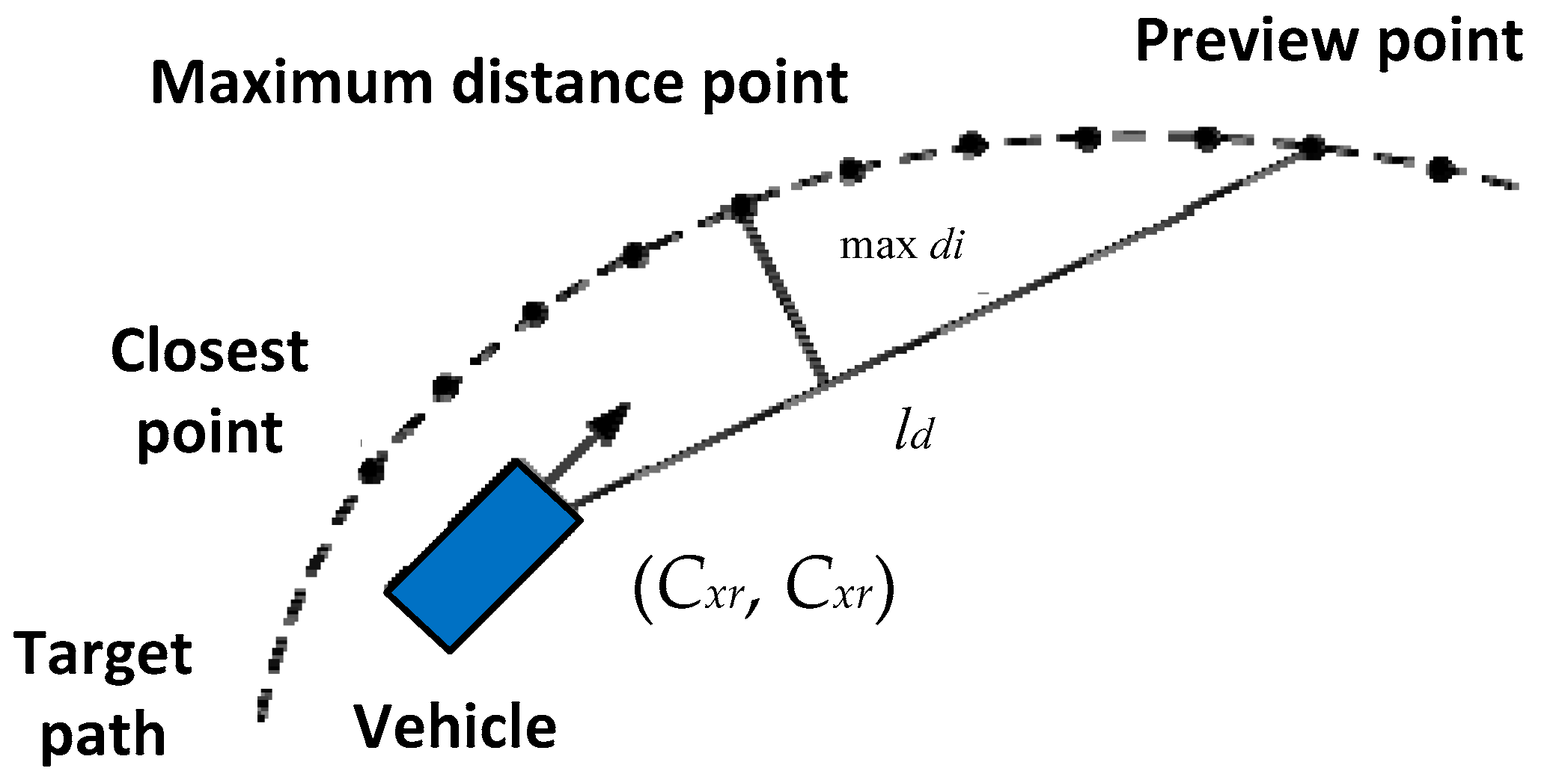
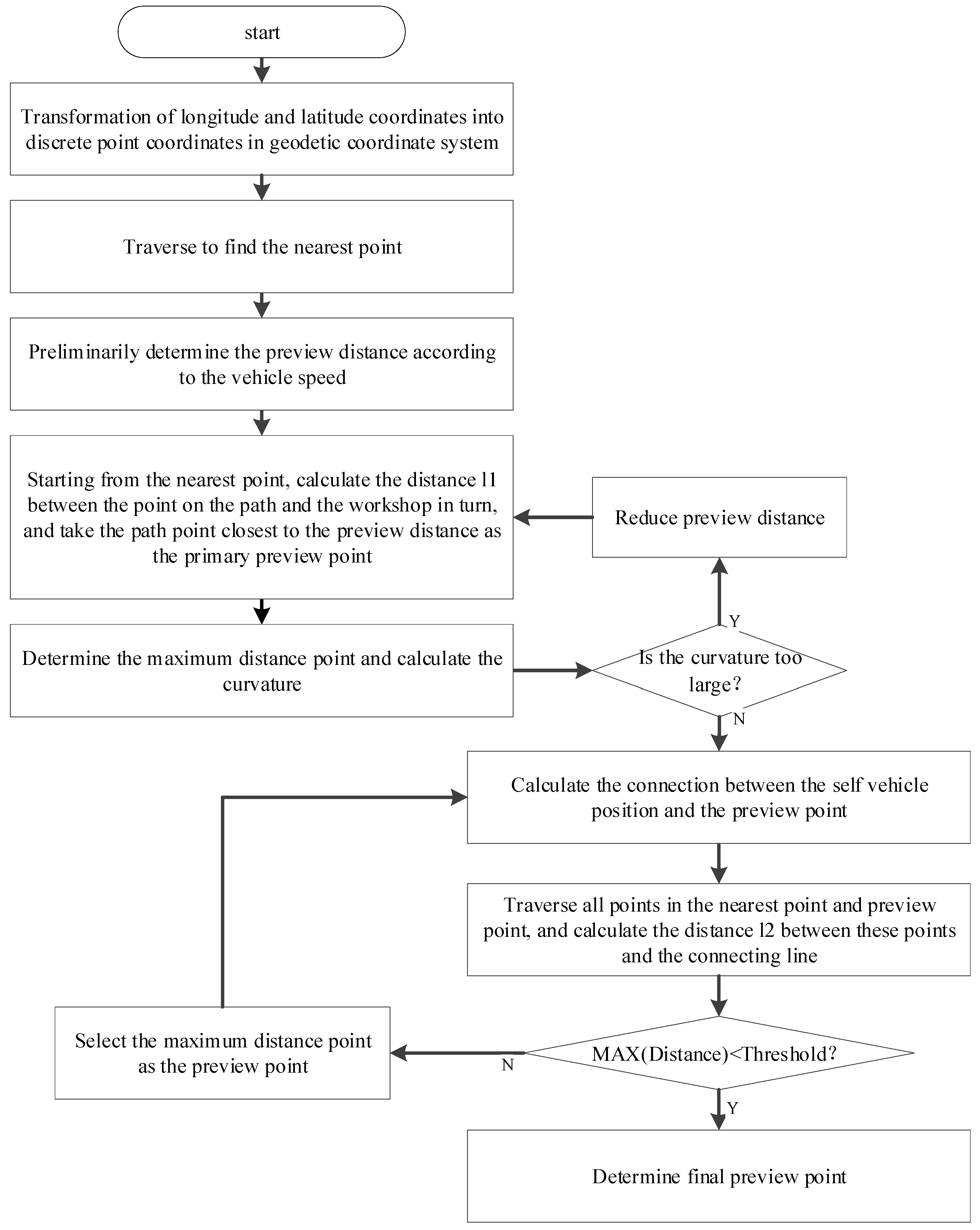
In this paper, a single-point preview method, considering curvature, is used to calculate the preview point, as shown in Figure 2.
(1)
According to the GPS information of the path, the nearest point of the vehicle position at the current moment is determined after coordinate transformation. According to Formula (1), the following formula is obtained after simplification and operation processing, and the nearest point is found by traversing the following formula:
{ D i s Y = ( l a t p l a t v ) 111000 D i s X = ( l o n p l o n v ) 111000 cos ( l a t v 0.01745 )
where latp and lonp are the latitude and longitude coordinates of the path points; latv and lonv are the latitude and longitude coordinates of the self-driving vehicle. After obtaining DisX and DisY, D i s X 2 + D i s Y 2 is used to calculate the distance between the discrete points on the expected path and the self-workshop.
(2)
The preview distance is determined according to the following formula:
l d = { k V t , k V t > l d _ m i n l d _ m i n , k V t l d _ m i n
Vt is the vehicle speed, k is the proportional coefficient, and ldmin is the minimum preview distance.
(3)
Find the coordinates of the nearest point according to the method described in step 1, calculate the distance between the point on the path and the vehicle from the nearest point, take the path point closest to the preview distance as the preview point, return the coordinates of that point, and then obtain the pre-selected preview point.
(4)
After the preview point is determined, the line between the current vehicle position (Cxr, Cxr) and the preview point is calculated.
(5)
Traverse all the points in the nearest point and preview point, calculate the distance between these points and the line in step 4, and then determine the maximum distance point.
(6)
Determine whether the distance maxdi between the maximum distance point and the line in step 4 exceeds the threshold, and then judge whether the preselected preview point is reasonable. The curvature value does not need to be calculated specifically, and the curvature can be reflected by judging the distance between the maximum distance point and the line in step 1.
(7)
If step 3 determines that the threshold value is exceeded, the current maximum distance point is selected as the preselected preview point, and steps 1–3 are repeated until the requirements are met, and the preselected preview point is output as the preview point.
The pseudo code of one of the above procedures is shown in the Figure 3:
The minimum value of x and its location is represented by fmin(x), ffit((x1,y1),(x2, y2)) is used to fit a straight line according to two points, and fdis is the distance from the point to the line. The final output (x(maxdisIndex), y(maxdisIndex)) is the preview point coordinates after the above process cycle judgment is repeated many times.

3. Lateral Motion Control Based on Variable Universe Fuzzy Sliding Mode

Considering the complex working environment of a military unmanned vehicle, and the strong coupling relationship between the steering system and chassis components, sliding mode control with strong robustness adaptability, and no dependence on the accuracy of the model, is very suitable for the lateral motion control algorithm. At present, the chattering phenomenon has been solved, to a certain extent, within which the use of FSMC is more common. Compared with other deep learning algorithms, such as neural networks, fuzzy control has the advantage of adaptive approximation and no need of accurate prior knowledge, which makes it easier to be widely used.

3.1. Calculation of Expected Steering Angle Based on Pure Tracking Algorithm

Whether it is manually input or collected in advance, the final actual path information is a series of GPS longitude and latitude coordinate points. Therefore, these longitude and latitude coordinates (lon, lat) need to be converted first, and then the discrete coordinate points (X, Y) in the geodetic coordinate system are obtained.
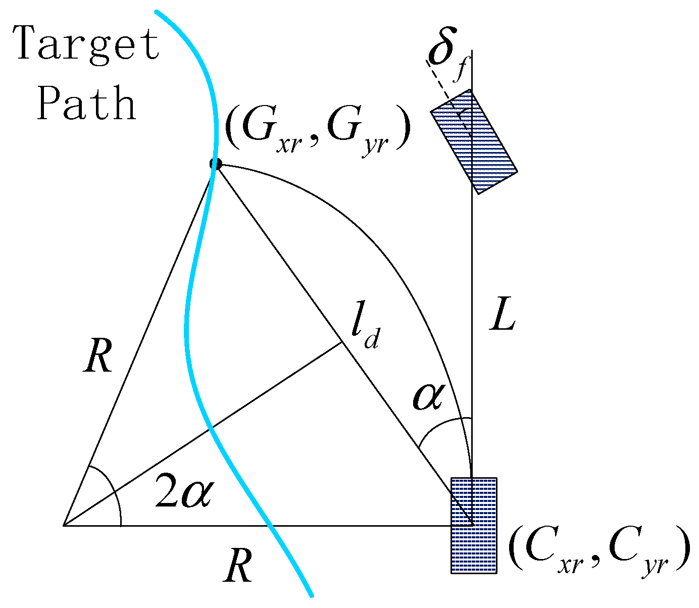
Specifically, the coordinate of the center point of the rear axle of the unmanned vehicle is set as ( C x r , C y r ) in the geodetic coordinate system, and the coordinates of the preview point (i.e., target point) are ( G x r , G y r ) , The front wheel angle of the unmanned vehicle is δ f , and the current turning radius is R. As shown in Figure 4, according to the principle of plane geometry, the following applies:
2 R sin α = l d
where l d represents the distance between the center point of the rear axle and the preview point, that is, the preview distance;   α is the angle between the UAV heading and preview line, and its value can be solved by the following formula:
α = arcsin ( G y r C y r l d ) φ p v
where φ p v is the heading angle of the unmanned vehicle.
According to Ackermann’s steering principle, the following is true:
tan δ f = L / R
where L represents the wheelbase of the unmanned vehicle.
By substituting Formulas (5) and (6) into Equation (7), we obtain the following:
tan δ f = 2 L sin α / l d
The control law of the pure tracking controller can be obtained by transforming Formula (8), as follows:
δ f = arctan ( 2 L sin α / l d )
δ f is the input δ of the motion control system. In particular, for the pure tracking controller, the selection of preview distance l d is particularly important to the performance of the controller. In practical applications, the preview distance needs to be adjusted by a large number of tests. The basic calculation formula is shown in the formula of preview distance (Formula (5)) in Section 1 of this paper. After obtaining the expected angle by the pure tracking algorithm, the actual vehicle rotation angle is obtained by using the variable universe FSMC algorithm.

3.2. Design of Sliding Mode Controller

Assuming that the front wheel of the vehicle turns by a small angle, the vehicle dynamic equation can be described as follows:
{ m v ˙ y + m v x β = F y f + F y r I z ω ˙ = a F y f b F y r
In Equation (11), v x represents the longitudinal speed of the vehicle, v y is the lateral speed, m is the mass of the whole vehicle, ω represents the yaw rate of the vehicle, lf and lr are the distance from the front and rear wheels to the vehicle centroid, respectively, F x f and F y r represent the lateral forces of the front and rear wheels, respectively, β is the side slip angle of the mass center, and I z is the moment of inertia to the center of mass of the vehicle. When the tire is in a linear region, the relationship between the lateral force and the tire can be approximately expressed as follows:
{ F y f α f C f F y r α r C r
Cf and Cr are the lateral stiffness of the front and rear wheels, respectively. The side slip angle of the front and rear wheels of the vehicle can be expressed as follows:
{ α f v y v x + a ω v x δ α r v y v x b ω v x
In the case of a small center of mass, the steering angle of the front wheel can be approximately expressed as follows: β = v x / u . The 2-DOF vehicle model equation about yaw rate ω and β can be obtained by Formulas (5)–(7) simultaneously, as follows:
{ ω ˙ = l f 2 C f + l r 2 C r I z v x ω + l f C f l r C r I z β l f C f I z δ β ˙ = ( l f C f l r C r M v x 2 1 ) ω + C f + C r M v x β C f M v x δ
As shown in Figure 5, for an uncertain system, when the system is subject to both internal parameter perturbation and external disturbances, the system state equation can be expressed as follows:
x ˙ = A x + B [ u ( t ) + E ( t ) ]
where A and B are parameter perturbations within the system, x is the state quantity, u is the control quantity, and E ( t ) includes the uncertainty and external disturbance of the system.
According to Formula (8), the following can be concluded:
x = [ ω β ] ,   A = [ a 11 a 21 a 12 a 22 ] ,   B = [ b 11 b 21 ]
where a 11 = l f 2 C f + l r 2 C r I z v , a 21 = l f C f l r C r M v x 2 1 , a 12 = l f C f l r C r I z , a 22 = C f + C r M v x , b 11 = l f C f I z , b 21 = C f M v x .
Therefore, the state equation of the controlled system studied in this paper can be expressed as follows:
x ˙ = f ( ω r , β ) + b 11 [ u ( t ) + E ( t ) ]
where f ( ω r ) can be expressed by the side slip angle of the center of mass and the yaw rate, as follows:
f ( ω r , β ) = a 11 ω r + a 12 β
The gain of reaching law of sliding mode control is selected as follows:
K ( t ) = max ( | E ( t ) | ) + η
where η > 0 .
Because the side slip angle of the center of mass cannot be directly controlled, and the ideal value and the actual value of the side slip angle of the center of mass cannot be directly controlled, the ideal value of the side slip angle of the center of mass will have a large error when the vehicle is unstable. Moreover, the yaw rate can reflect the overall movement trend of the vehicle better than the wheel angle. Therefore, the difference between the actual yaw rate and the ideal yaw rate is selected as the tracking error of the system.
e = ω r ω d
The ideal yaw rate ω d in Equation (19) is calculated according to the expected angular value and the 2-DOF model; ω r is the actual yaw rate. The switching function of the controller is selected using the following equation:
s = e + λ 0 t e ( t ) d t
By deriving the switching function, we can obtain the following results:
s ˙ = e ˙ + λ e = ω ˙ r ω ˙ d + λ ( ω r ω d )
The sliding mode control law is designed as follows:
u = 1 b 11 [ f ( ω r ) + ω ˙ d + λ ( ω r ω d ) + K ( t ) sgn ( s ) ]
The Lyapunov theorem is used to prove the stability of the designed lateral sliding mode controller, as follows:
V = 1 2 s 2
The derivation of Equation (23) shows the following:
V ˙ = s s ˙ = s [ e ˙ + λ e ] = s [ f ( ω r ) + b 11 [ u ( t ) + E ( t ) ] + ω ˙ d + λ e ]
The sliding mode control law of Equation (22) is substituted into Equation (24) to obtain the following:
V ˙ = s [ K ( t ) sgn ( s ) E ( t ) ] = K ( t ) | s | E ( t ) s η | s |
where η > 0 , the designed controller meets the stability requirements.
By substituting f ( ω r ) into Equation (21), the expression composed of parameters of the vehicle dynamic model can be obtained as follows:
s ˙ = l f 2 C f + l r 2 C r I z v ω r l f C f I z δ ω ˙ d + λ ( ω r ω d )
Let s ˙ = 0 . According to the hypothesis, we can know the yaw acceleration ω ˙ d = 0 at this time. Therefore, the control input front wheel angle can be expressed as follows:
δ = I z l f C f [ l f 2 C f + l r 2 C r I z v ω r ω ˙ d + λ 0 ( ω r ω d ) ]
By substituting Formula (22), we obtain the following:
δ d = δ + K ( t ) sgn ( s )
K ( t ) is the rate of the system moving point approaching the switching surface; when K ( t ) is larger, the speed of the approaching moving point will be faster, and the response speed of control will be faster, but it will also cause greater jitter. Therefore, the jitter of the sliding mode control is mainly caused by the reaching term K ( t ) sgn ( s ) ; in order to ensure the control effect of the sliding mode controller, it is necessary to further optimize it.

3.3. Design of Fuzzy Sliding Mode Controller

According to Equation (28), it can be observed that the existence of the symbolic function can effectively eliminate the unknown interference, but it inevitably leads to chattering. Therefore, this paper uses adaptive fuzzy control, based on switching fuzzification, to improve the trajectory of the system near the sliding surface, which not only enables the system to adapt to various working conditions, but also enables good elimination of different interference intensities. By using fuzzy approximation, the discrete symbolic function can be continuous, which can effectively reduce the chattering phenomenon. Therefore, a variable switching gain is designed in this paper. Fuzzy rules are used to adjust the switching gain according to the relative position and movement trend of the system and sliding surface.
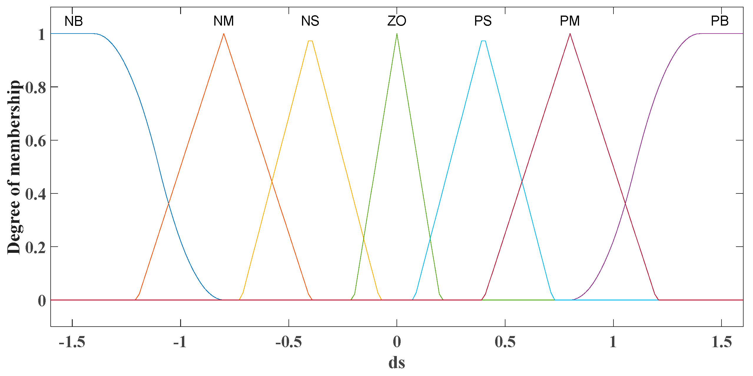
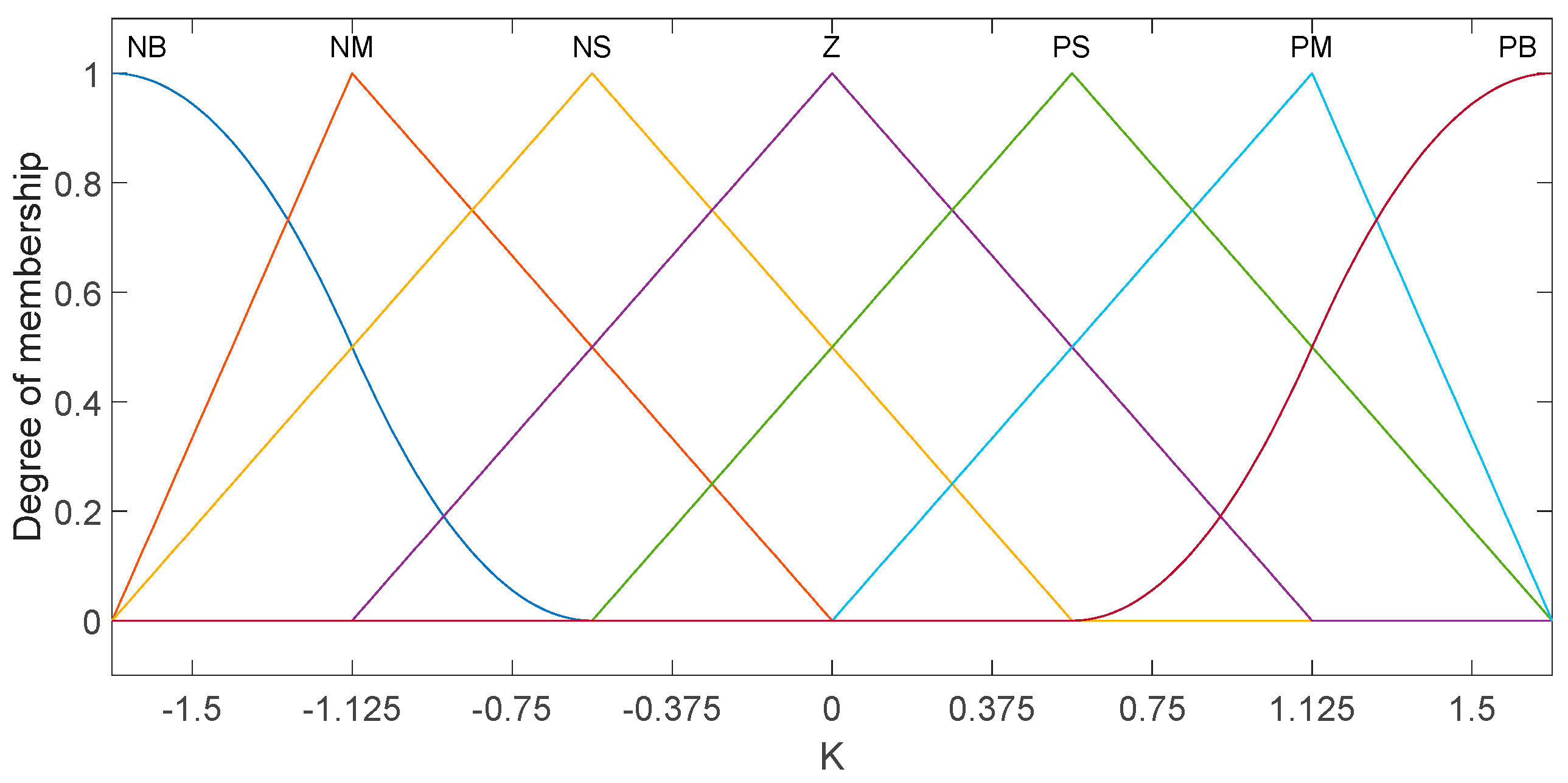
Taking s and s ˙ as the fuzzy input, and k as the output, the corresponding fuzzy linguistic variables are {NB NM NS ZO PS PM PB}. If s s ˙ > 0, the current state of the sliding mode function is the same as the change trend, and there is a trend far away from the sliding surface, the switching gain k(t) should be increased at this time. If s s ˙ < 0, then the state of the sliding mode function is opposite to the change trend, and the system is approaching the sliding surface, so the switching gain k should be reduced. At the same time, the size of | s s ˙ | also needs to be considered, so as to further design fuzzy rules reasonably. When s s ˙ is large, |k| should also have a larger change; otherwise, the change should be reduced.
In the design of the fuzzy controller, the design of fuzzy rules is an important part to determine its performance (Table 1).
The output y(x) of the fuzzy system can be written as the product inference engine, single-valued fuzzy controller, and center average defuzzer, as follows:
y ( x ) = j = 1 m y j ( i = 1 n μ A i j ( x i ) ) j = 1 m ( i = 1 n μ A i j ( x i ) )
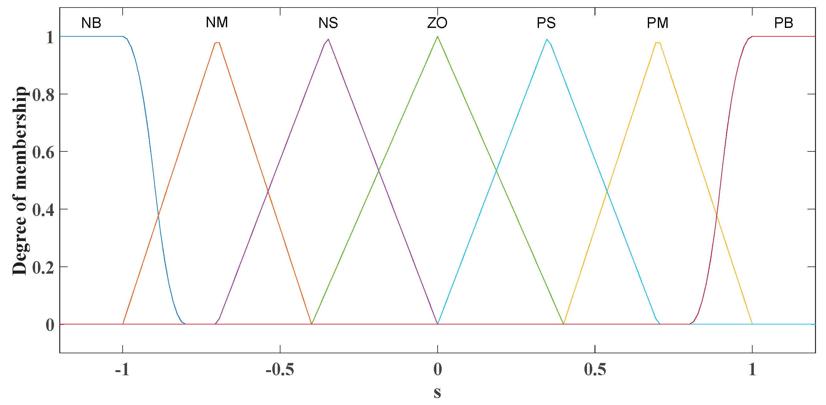
In this section, the switching function s(t) is used as the input of the fuzzy system. In this section, the switching function is used as the output of the fuzzy system, where A i j is its fuzzy set {NB NM NS ZO PS PM PB}, μ A i j ( s i ) is the membership function of si, where μ N B adopts the Z-type membership function, μ P B adopts the S-type membership function, and the others adopt the triangle membership function; the membership function is shown in the following Figure 6, Figure 7 and Figure 8.

3.4. Design of Variable Universe Fuzzy Sliding Mode Controller

According to the principle of fuzzy control, if the fuzzy system is to approach a changing function infinitely accurately, it needs infinite fuzzy rules to realize in theory, which is almost impossible to complete. Therefore, under the premise that the number of rules and membership functions remain unchanged, further accurate approximation can be achieved by adaptive adjustment of the universe.
In this paper, the exponential expansion factor in the function model is selected to adjust the fuzzy universe of three variables adaptively.
α ( x ) = 1 - λ e ( - 0 . 5 x 2 ) λ ( 0 , 1 )
where λ is the scale factor, which determines the degree of scaling. Parameter x is the input, such as s, s , ˙ or k.
In this paper, the expansion factor λ of the input universe is 0.6, and that of the output universe is 0.3. Since the expansion factors of the input and output domains are all reduced, it is necessary to adjust the initial universe, designed in the previous section, so that the product of the adjusted universe and the expansion factor is centered on the initial universe. At the same time, because the fuzzy logic module in Matlab/Simulink cannot realize the variable universe, this paper uses the S-function module to design the variable universe fuzzy control, which replaces the original fuzzy logic module.

4. Simulation Analysis

To preliminarily verify the trajectory tracking control algorithm designed in this paper, based on the Simulink and CarSim joint simulation platform, the tracking algorithm is tested in a variety of working conditions. The road centerline is used to simulate the GPS path as the input of Simulink, and the front wheel rotation angle, obtained by algorithm processing, is the output to CarSim. The structure is shown in the Figure 9.
This paper mainly compares PID, traditional FSMC, and variable universe FSMC. The weakening of the chattering phenomenon is obvious, and is not the focus of this paper. Therefore, we will focus on the comparison of the effects before and after the variable universe. For the comparison of the weakening of the buffeting phenomenon, please refer to [26].

4.1. Oval Lane Test

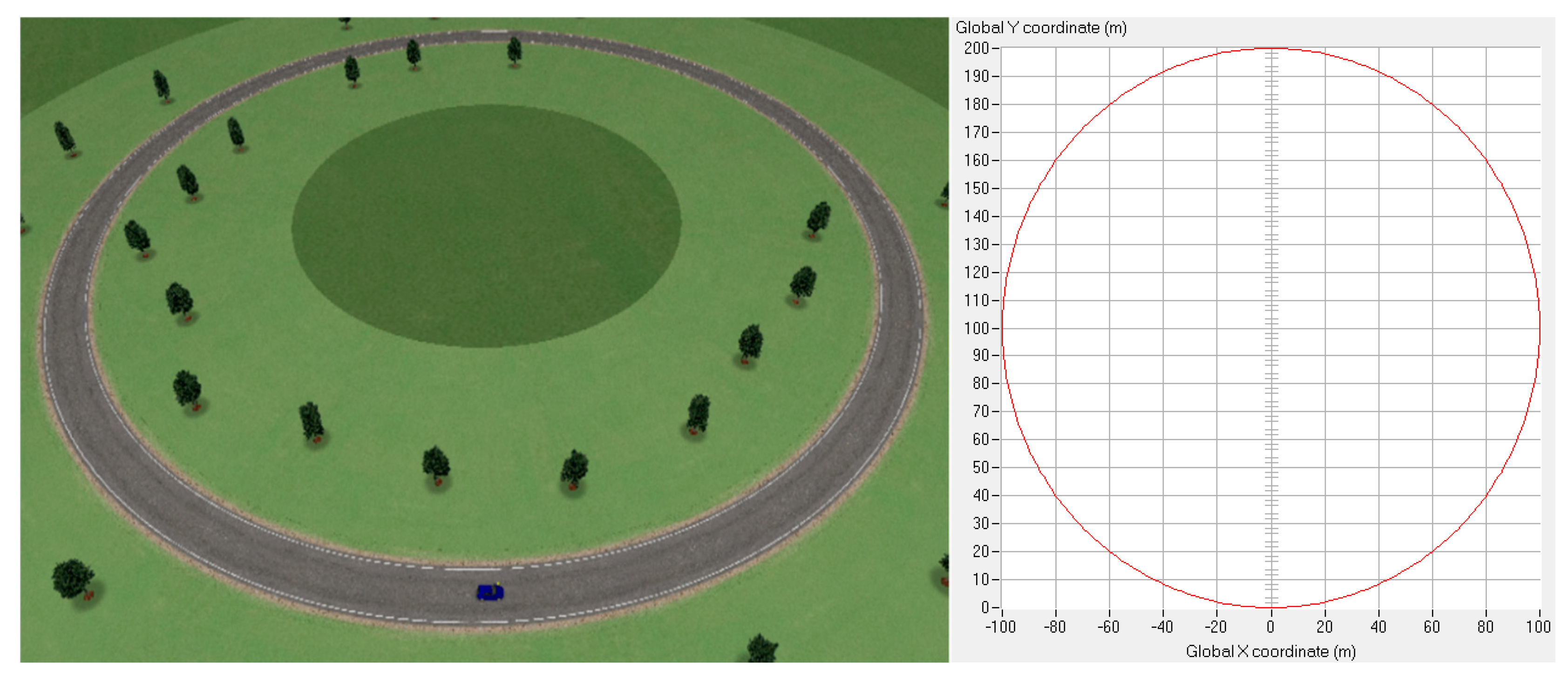
The ellipse lane can be used to test the rapidity (transient) and accuracy (steady state) of the lateral error convergence of vehicles in trajectory tracking. Its lane shape and parameters are shown in the Figure 10 and Figure 11.
In the simulation test under this condition, the average absolute lateral error of the vehicle under the control of the variable universe FSMC algorithm is 0.0089 m, which is far less than the 0.2025 m of PID and 0.1499 m of FSMC. Compared with the FSMC algorithm, the PID algorithm can stabilize rapidly after a long period of oscillation, and, finally, keep a lateral deviation of about 0.5 m. Although the FSMC algorithm can be effectively adjusted, the control accuracy is obviously not as good as that of the variable universe FSMC, and the final error is about 0.2 m. Therefore, both the fast convergence performance in transient state and the adjustment accuracy in steady state are better than the other two algorithms.

4.2. FHWA Lane Test

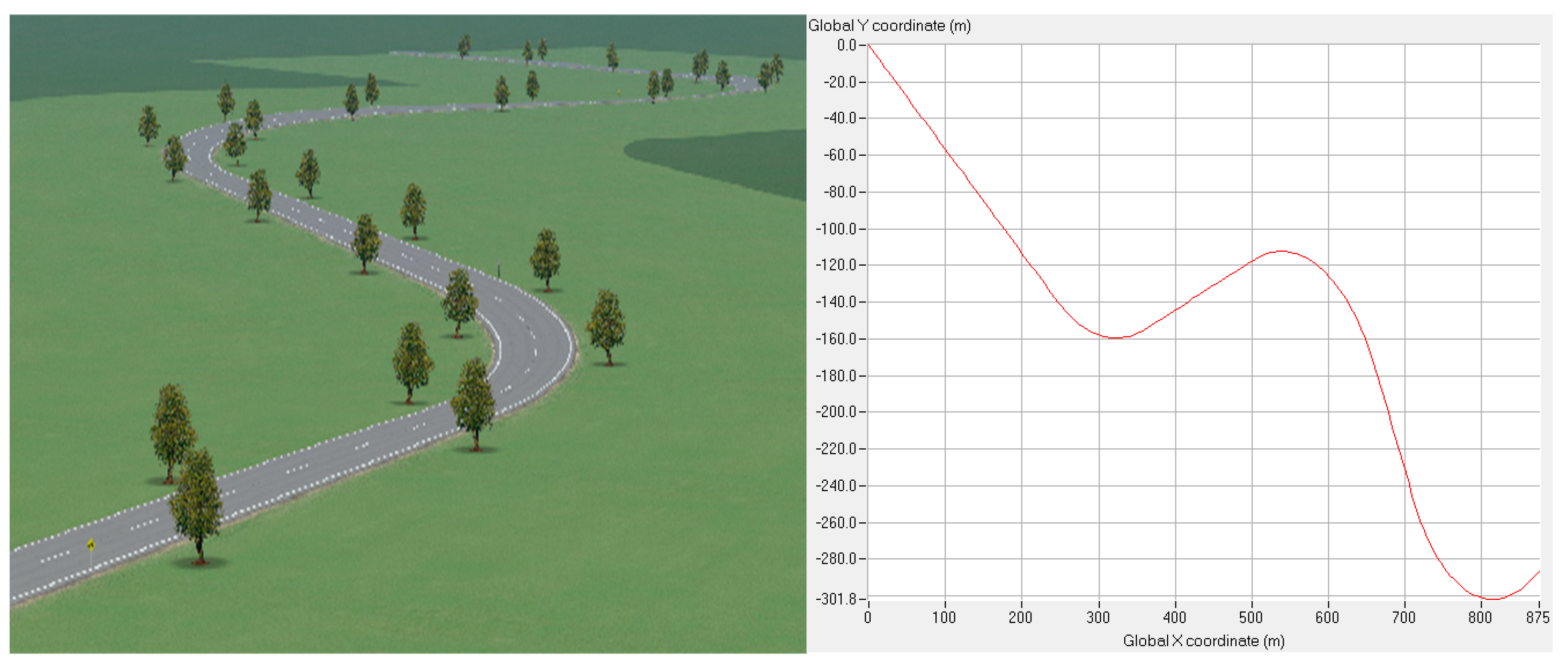
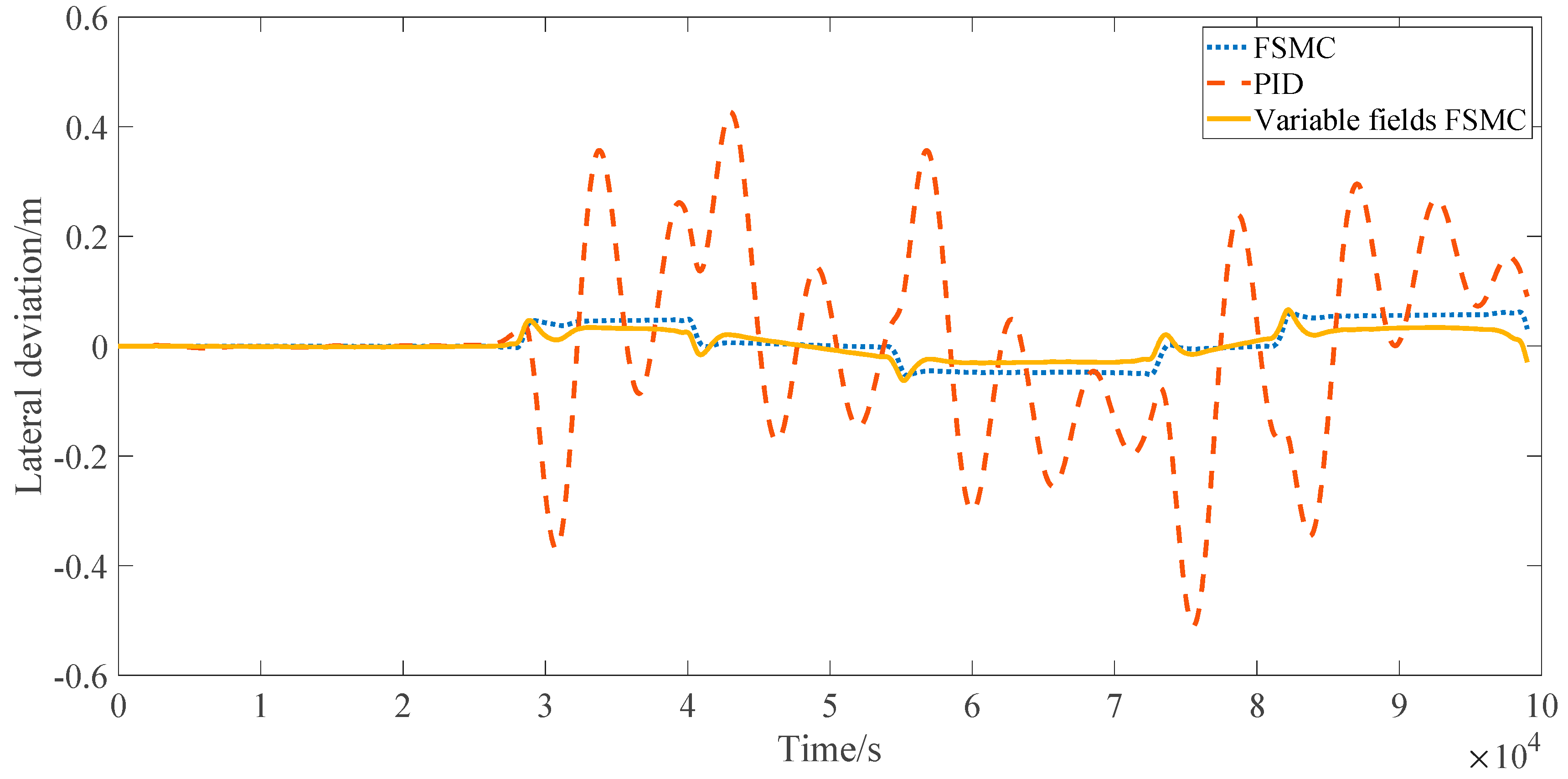
Similarly to the double-lane change condition, the Federal Highway Administration (FHWA) has developed a more stringent test path, as shown in the Figure 12 and Figure 13.
In the simulation test under this condition, the average absolute lateral error under the control of the variable universe FSMC algorithm is 0.0173 m, which is far less than the 0.1212 m under the PID method and 0.0248 m under the FSMC algorithm. From the perspective of the control process, the variable universe FSMC can converge to zero error faster because of the continuous adjustment of the universe, and can be closer to zero error than FSMC in most cases, and the adjustment is more accurate.

4.3. “8” Lane Test

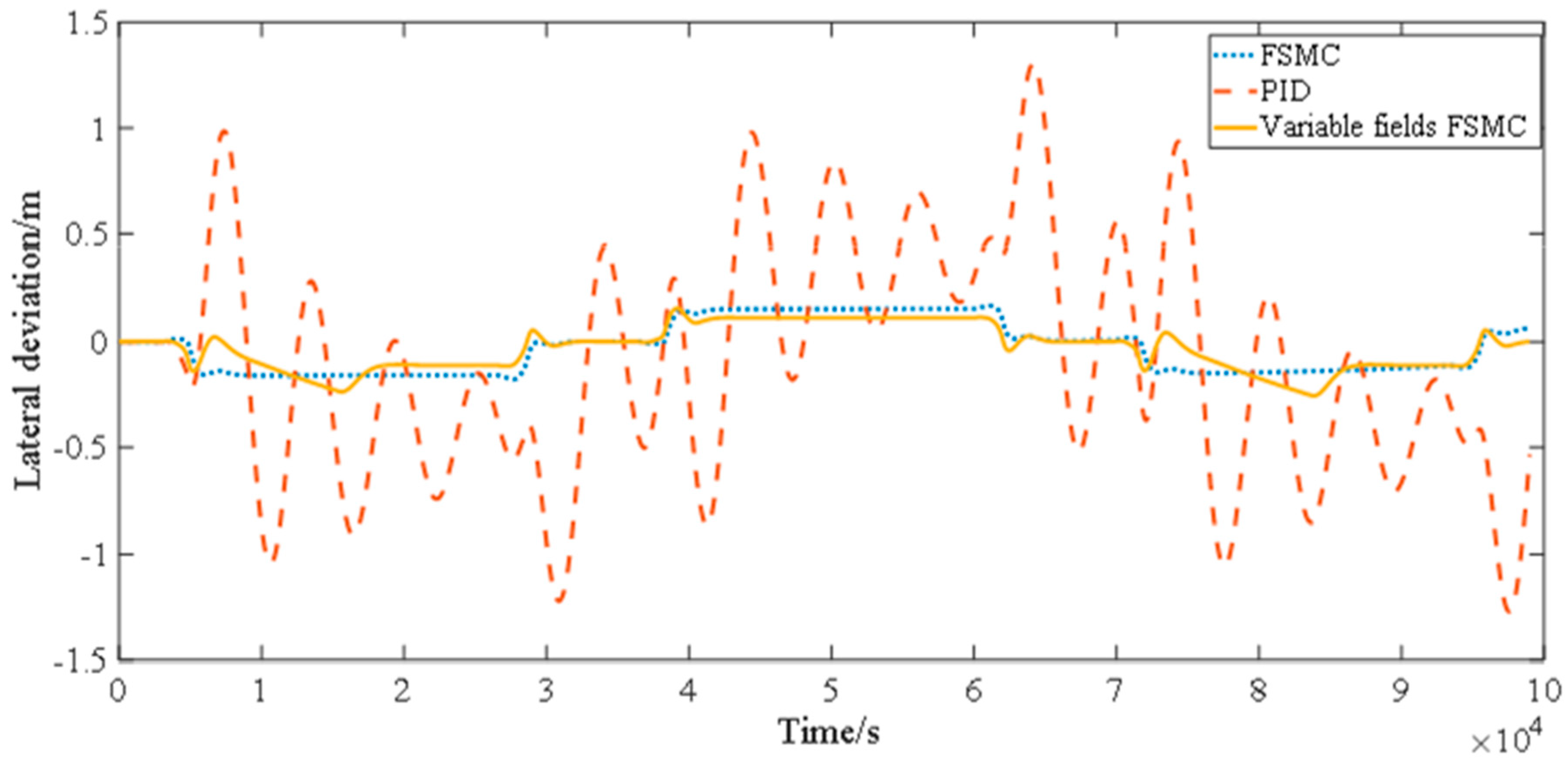
The “8” lane test can assess the following performance of vehicles under continuous and large-scale curves. The structure of the “8” lane test is shown in Figure 14 and Figure 15.
In the simulation test under this condition, the average absolute lateral error under the control of the variable universe FSMC algorithm is 0.0883 m, which is far less than the 0.4601 m under the PID method and 0.1846 m under the FSMC method. It can be observed that when the FSMC is close to zero error, it will not be fine-tuned. This is due to the setting of fixed fuzzy universe, which makes the input error map to the minimum fuzzy language variable. To avoid frequent chattering, the error is not adjusted, so that the system cannot finally approach zero. The improved variable universe FSMC enables the system to make subtle changes without chattering, which greatly improves the accuracy of system control.

4.4. Real Vehicle Test

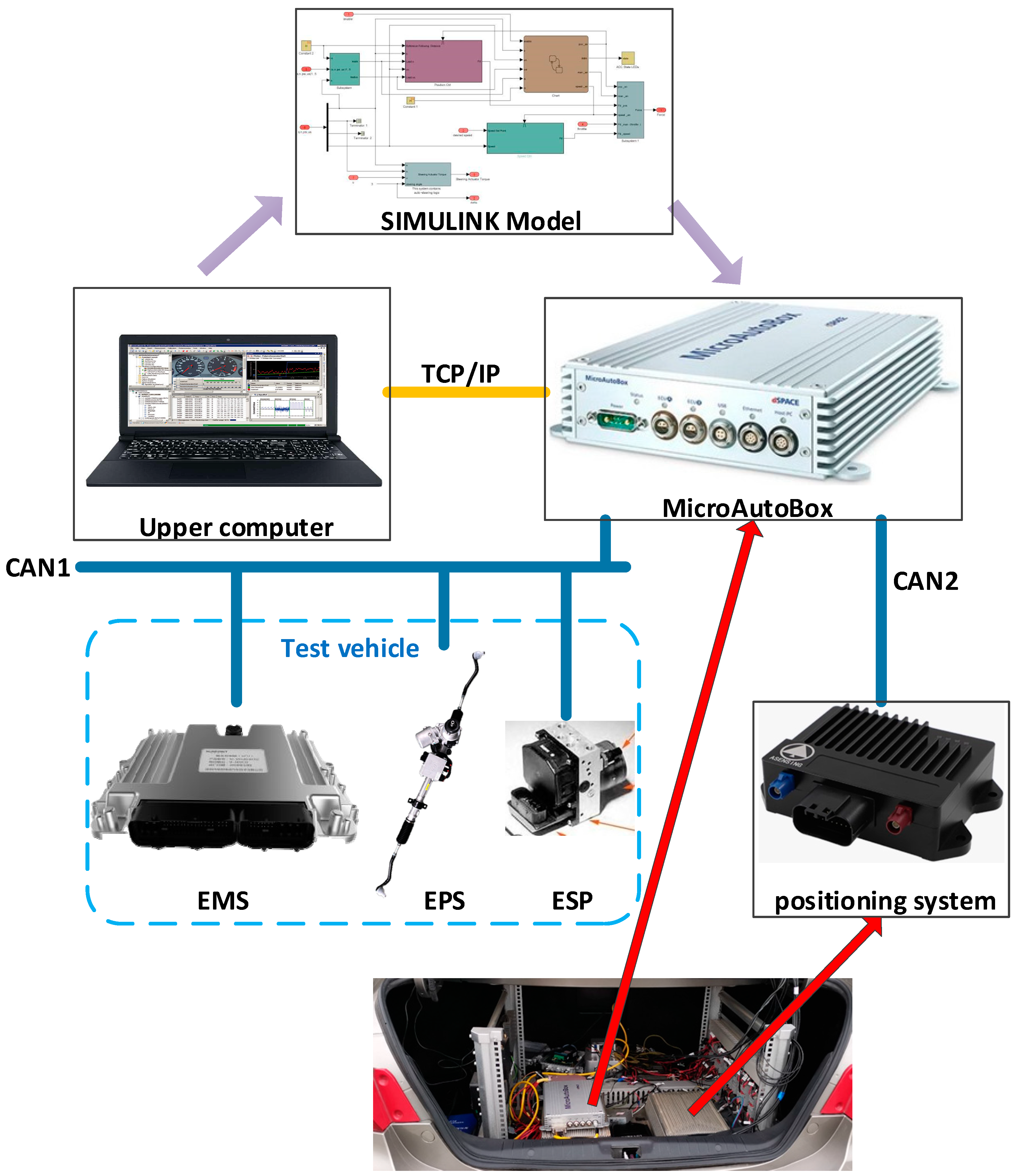
The speed, acceleration, wheel speed and other basic state signals of the vehicle, acceleration/deceleration, and steering control are transmitted through the power CAN bus of the original vehicle, and the positioning information of the high-precision GPS positioning equipment is transmitted through another CAN. Finally, the analysis of the CAN message is completed in the built model, and the real-time vehicle status is fed back to the model and controlled. The control algorithm model built in this paper is compiled and generated, and runs in MicroAutobox. The data information interaction between MicroAutobox and the upper computer is carried out through TCP/IP. Finally, the control desk software on the test PC is used for debugging, calibration, and user interaction. The whole shown in Figure 16.
The transformation part of the communication system is shown in Figure 16. The test vehicle used in this project has the body CAN and the power CAN. In the test, the power CAN is mainly used to obtain the vehicle running state parameter information, such as the wheel speed, steering angle, and gear position. High-precision GPS integrated navigation also uses the CAN interface for communication. The two CAN buses of vehicle power CAN and the GPS positioning system are connected to the two-way CAN of MicroAutobox, respectively. MicroAutobox analyzes the CAN data of each channel by running the pre-burned model, so as to obtain the required relevant state quantity to provide real-time vehicle feedback information.
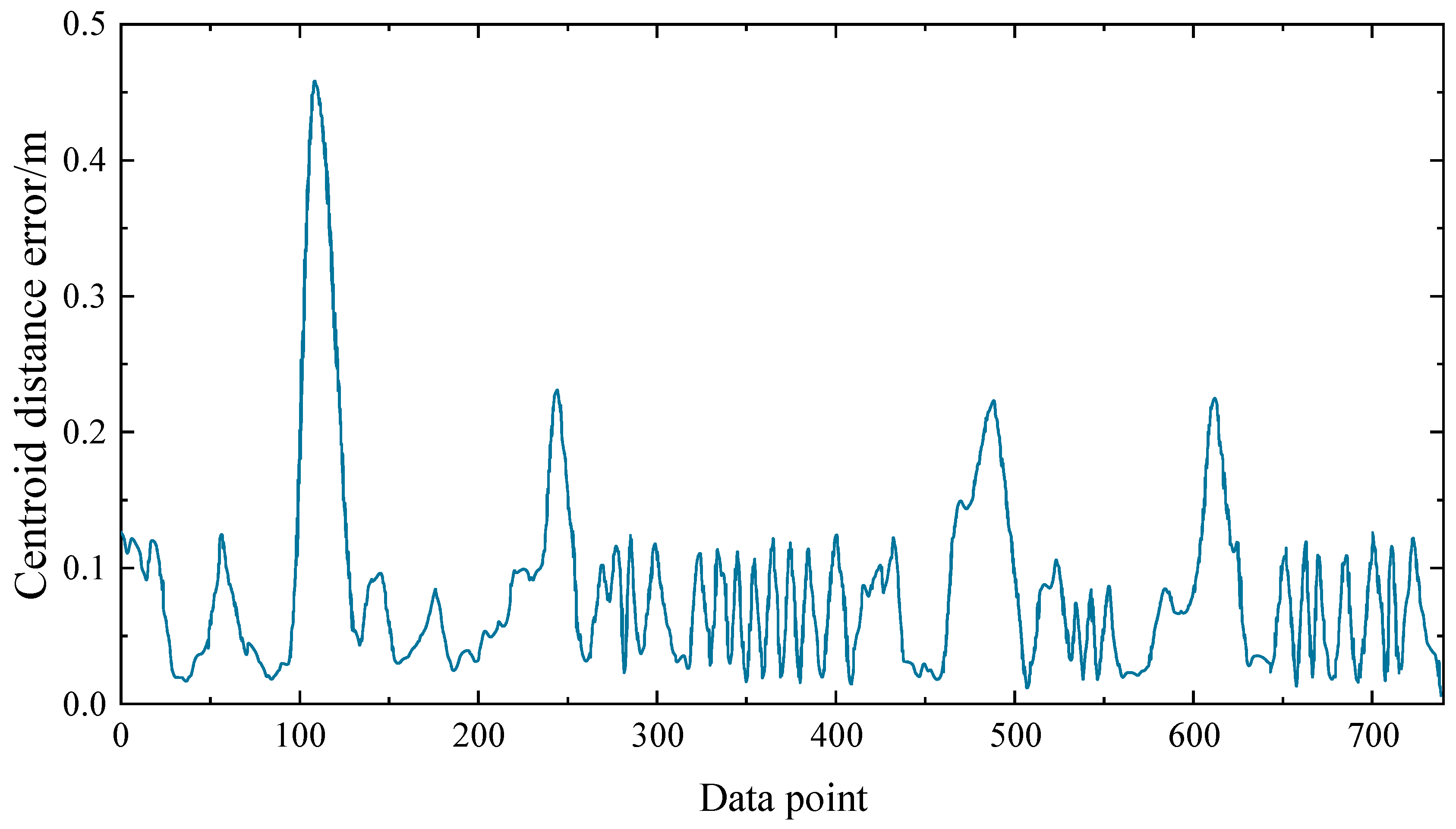
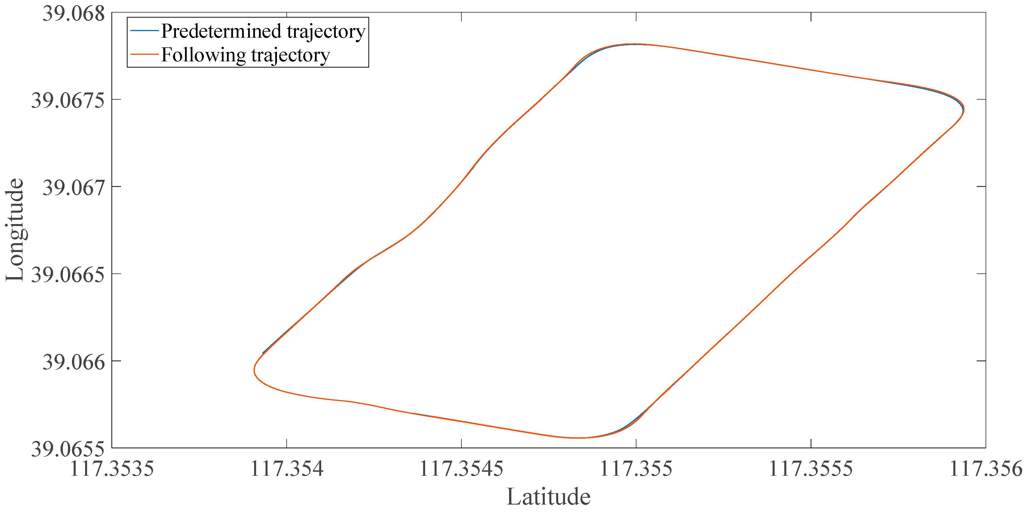
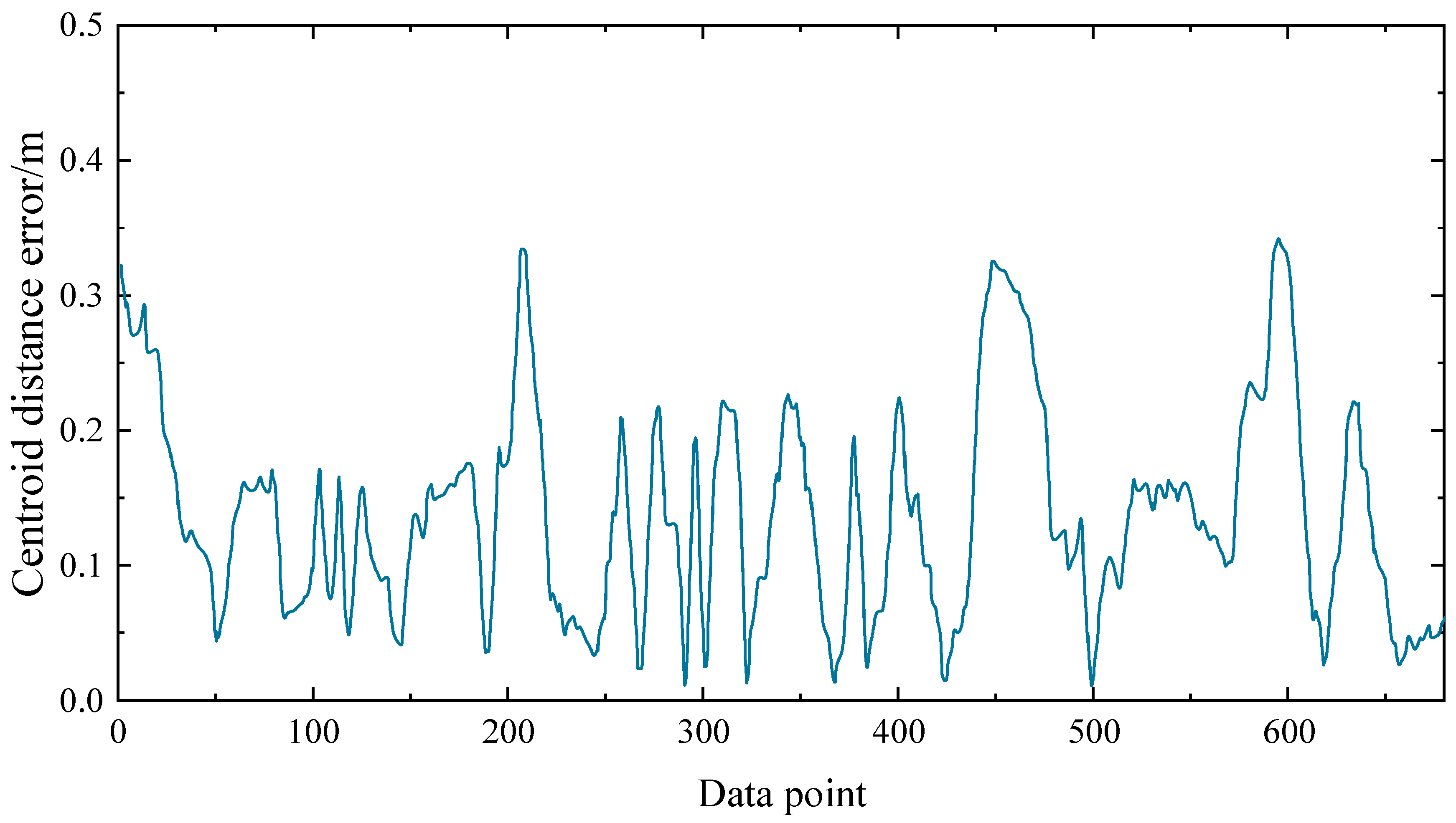
To further test the performance of the algorithm, the real vehicle test is carried out in two cases of rectangular field turning left and rectangular field turning right, as shown in the figure below. To more intuitively compare the error size at different times, this paper selects the absolute value of the error as the measurement index, stores the GPS coordinates of the predetermined track and the GPS coordinates of the following track, and draws the trajectory comparison chart and the lateral error comparison chart, respectively, as shown in Figure 17, Figure 18, Figure 19 and Figure 20.
It can be observed, from the error diagram in Figure 18 and Figure 20, that the algorithm keeps the lateral error (absolute value) of the vehicle within 0.5 m, while four large “wave peaks” are generated in the whole running process, which correspond to the four right angle bends of the rectangular track. Although the error is larger than that of straight line driving, it can still ensure high tracking accuracy on the whole.

5. Conclusions

Firstly, the optimal preview point is obtained according to the data points of the differential GPS signal. The curvature is reflected from the side, by the calculation of the maximum distance point, and the preview points are selected iteratively. Secondly, the pure tracking algorithm is used to calculate the expected steering angle. Finally, a variable universe fuzzy sliding mode controller is designed to control the lateral motion of the vehicle by measuring the deviation in yaw rate. The variable universe FSMC algorithm designed in this paper is superior to the traditional FSMC, in terms of the arrival time and the steady-state accuracy, and further optimizes the tracking accuracy of the system on the premise of weakening the chattering phenomenon. Due to the limited time and conditions, this paper only carries out the real vehicle test on the more conventional road, and does not test the effect of other control algorithms. In the future, the real vehicle test will be carried out on more roads and compared with other algorithms.

Author Contributions

Conceptualization, X.Y. and J.L.; methodology, J.L. and X.S.; software, J.L.; validation, X.Y., H.Z. and X.X.; formal analysis, X.Y. and J.L.; investigation, X.Y. and J.L.; resources, X.Y. and J.L.; data curation, X.Y.; writing—original draft preparation, J.L.; writing—review and editing, X.Y.; visualization, X.Y.; supervision, H.Z.; project administration, X.X.; funding acquisition, X.S. All authors have read and agreed to the published version of the manuscript.

Funding

National Key Research and Development Program of China under Grant 2018YFB0104803. Science and Technology Cooperation Program of Jiangsu Province with Hong Kong, Macau and Taiwan under Grant BZ2020050.

Institutional Review Board Statement

Not applicable.

Informed Consent Statement

Not applicable.

Acknowledgments

Thanks for the test conditions provided by China Automotive Technology & Research Center Co. Ltd. (Tianjin, China) for my experimental research.

Conflicts of Interest

There is no conflict of interest regarding the publication of this paper.

References

  1. Lu, W.; Dong, J.; Zhang, P. Research on vision enhancement system of military vehicle driver based on uncooled infrared detection technology. Appl. Opt. 2019, 40, 1033–1038. [Google Scholar]
  2. Xia, X.; Wang, H.; Li, X. Research on high precision automatic leveling control system of a military radar vehicle. Mech. Des. Manuf. 2019, 9, 158–160. [Google Scholar]
  3. Lu, H.; Xing, Y.; Zhuo, G. Review on Motion Control of Autonomous Vehicles. Available online: http://kns.cnki.net/kcms/detail/11.2187.th.20200416.1728.010.html (accessed on 6 June 2021). [CrossRef]
  4. Ding, N.; Ran, X.; Zhang, H. Driver model for single track vehicle based on single point preview optimal curvature model. J. Mech. Eng. 2008, 44, 220–223, 228. [Google Scholar] [CrossRef]
  5. Dong, T. Lane keeping system based on improved preview driver model. Pract. Automob. Technol. 2019, 24, 143–145. [Google Scholar]
  6. Ren, D.; Cui, S.; Wu, H. Preview control of lane keeping and its steady state error analysis. Automot. Eng. 2016, 38, 192–199. [Google Scholar]
  7. Xu, S.; Peng, H. Design, analysis, and experiments of preview path tracking control for autonomous vehicles. IEEE Trans. Intell. Transp. Syst. 2020, 21, 48–58. [Google Scholar] [CrossRef]
  8. Zhao, X.; Chen, H. A study on lateral control method for the path tracking of intelligent vehicles. Automot. Eng. 2011, 33, 382–387. [Google Scholar]
  9. Pan, Z. Research on Motion Control Approaches of Autonomous Vehicle in Urban Environments; University of Science and Technology of China: Hefei, China, 2012. [Google Scholar]
  10. Marino, R.; Scalzi, S.; Netto, M. Nested PID steering control for lane keeping in autonomous vehicles. Control. Eng. Pract. 2011, 19, 1459–1467. [Google Scholar] [CrossRef]
  11. Silva, M.; Garrote, L.; Moita, F. Autonomous electric vehicle: Steering and path-following control systems. In 2012 16th IEEE Mediterranean Electrotechnical Conference; IEEE: Manhattan, NY, USA, 2012; pp. 442–445. [Google Scholar]
  12. Guo, J.; Luo, Y.; Li, K. An Adaptive Hierarchical Trajectory Following Control Approach of Autonomous Four-Wheel Independent Drive Electric Vehicles. IEEE Trans. Intell. Transp. Syst. 2017, 19, 2482–2492. [Google Scholar] [CrossRef]
  13. Ackermann, J.; Guldner, J.; Sienel, W. Linear and nonlinear controller design for robust automatic steering. IEEE Trans. Control. Syst. Technol. 1995, 3, 132–143. [Google Scholar] [CrossRef]
  14. Yu, Z.; Zhang, X.; Xiong, L. Dynamic Control for Unmanned Skid-steering Vehicle with Conditional Integartors. J. Mech. Eng. 2017, 53, 29–38. [Google Scholar] [CrossRef]
  15. Tagne, G.; Talj, R.; Charara, A. Higher-order sliding mode control for lateral dynamics of autonomous vehicles, with experimental validation. In 2013 IEEE Intelligent Vehicles Symposium (IV); IEEE: Manhattan, NY, USA, 2013; pp. 678–683. [Google Scholar]
  16. Ji, X.; He, X.; Lv, C. Adaptive-neural-network-based robust lateral motion control for autonomous vehicle at driving limits. Control. Eng. Pract. 2018, 76, 41–53. [Google Scholar] [CrossRef]
  17. Falcone, P.; Borrelli, F.; Asgari, J.; Tseng, H.E.; Hrovat, D. Predictive Active Steering Control for Autonomous Vehicle Systems. IEEE Trans. Control. Syst. Technol. 2007, 15, 566–580. [Google Scholar] [CrossRef]
  18. Falcone, P.; Borrelli, F.; Tseng, H.E.; Asgari, J.; Hrovat, D. Linear time-varying model predictive control and its application to active steering systems: Stability analysis and experimental validation. Int. J. Robust Nonlinear Control. 2008, 18, 862–875. [Google Scholar] [CrossRef]
  19. Falcone, P.; Tseng, H.E.; Borrelli, F.; Asgari, J.; Hrovat, D. MPC-based yaw and lateral stabilisation via active front steering and braking. Veh. Syst. Dyn. 2008, 46, 611–628. [Google Scholar] [CrossRef]
  20. Gong, J.; Jiang, Y.; Xu, W. Model Predictive Control of Unmanned Vehicles; Beijing University of Technology Press: Beijing, China, 2014. [Google Scholar]
  21. Guo, H.; Liu, J.; Cao, D.; Chen, H.; Yu, R.; Lv, C. Dual-envelop-oriented moving horizon path tracking control for fully automated vehicles. Mechatronics 2018, 50, 422–433. [Google Scholar] [CrossRef] [Green Version]
  22. Kim, E.; Kim, J.; Sunwoo, M. Model predictive control strategy for smooth path tracking of autonomous vehicles with steering actuator dynamics. Int. J. Automot. Technol. 2014, 15, 1155–1164. [Google Scholar] [CrossRef]
  23. Nam, H.; Choi, W.; Ahn, C. Model predictive control for evasive steering of an autonomous vehicle. Int. J. Automot. Technol. 2019, 20, 1033–1042. [Google Scholar] [CrossRef]
  24. Ge, S.S.; Lee, T.H.; Hang, C.C.; Zhang, T. Stable Adaptive Neural Network Control; Kluwer Academic Publishers: New York, NY, USA, 2001. [Google Scholar]
  25. Wai, R.-J.; Lin, C.-M.; Hsu, C.-F. Adaptive fuzzy sliding-mode control for electrical servo drive. Fuzzy Sets Syst. 2004, 143, 295–310. [Google Scholar] [CrossRef] [Green Version]
  26. Zhang, H.; Liang, J.; Jiang, H.; Cai, Y.; Xu, X. Stability Research of Distributed Drive Electric Vehicle by Adaptive Direct Yaw Moment Control. IEEE Access 2019, 7, 2169–3536. [Google Scholar] [CrossRef]
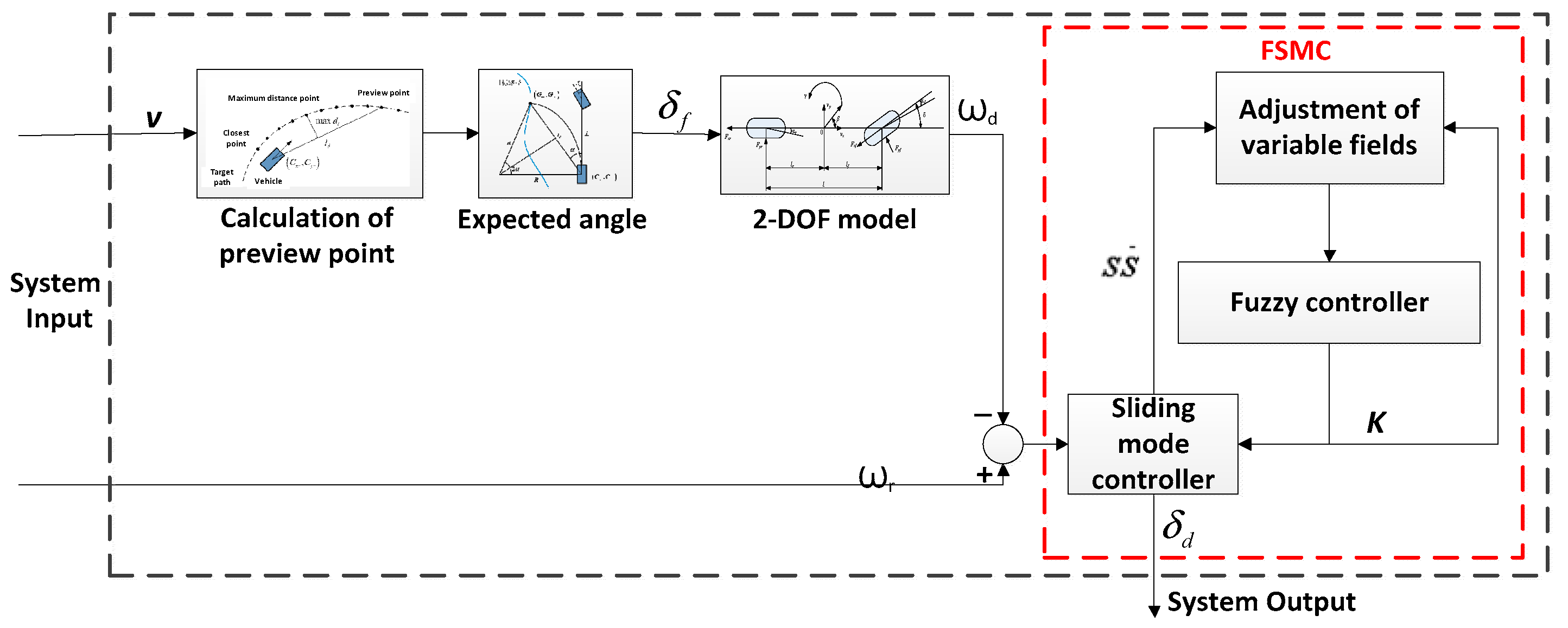
Figure 1. Preview FSMC system layout.
Machines 09 00304 g001
Figure 2. Schematic diagram of preview point screening.
Machines 09 00304 g002
Figure 3. Judgment and selection of preview points.
Machines 09 00304 g003
Figure 4. Schematic diagram of pure tracking algorithm.
Machines 09 00304 g004
Figure 5. Two degree of freedom dynamic model of vehicle.
Machines 09 00304 g005
Figure 6. S membership function diagram.
Machines 09 00304 g006
Figure 7. dS membership function diagram.
Machines 09 00304 g007
Figure 8. K membership function diagram.
Machines 09 00304 g008
Figure 9. Overall architecture layout of simulation verification test.
Machines 09 00304 g009
Figure 10. Oval lane.
Machines 09 00304 g010
Figure 11. Comparison of simulation results under elliptical lane.
Machines 09 00304 g011
Figure 12. FHWA lane.
Machines 09 00304 g012
Figure 13. Comparison of simulation results under FHWA lane.
Machines 09 00304 g013
Figure 14. “8” lane.
Machines 09 00304 g014
Figure 15. Comparison of simulation results under “8” lane.
Machines 09 00304 g015
Figure 16. System architecture.
Machines 09 00304 g016
Figure 17. Comparison of rectangular right turns.
Machines 09 00304 g017
Figure 18. Comparison of rectangular right turns errors.
Machines 09 00304 g018
Figure 19. Comparison of rectangular left turns.
Machines 09 00304 g019
Figure 20. Error chart of rectangular left turns errors.
Machines 09 00304 g020
Table 1. Fuzzy rule table.
s ˙ . NBNMNSZOPSPMPB
k
s
NBNBNBNMZOPMPBPB
NMNBNMNSZOPSPMPB
NSNMNSNSZOPSPSPM
ZOZOZOZOZOZOZOZO
PSPMPSPSZONSNSNM
PMPBPMPSZONSNMNB
PBPBPBPMZONMNBNB
Publisher’s Note: MDPI stays neutral with regard to jurisdictional claims in published maps and institutional affiliations.