Article

Modeling the Dynamics of a Gyroscopic Rigid Rotor with Linear and Nonlinear Damping and Nonlinear Stiffness of the Elastic Support

by
Zharilkassin Iskakov
1,*,
Kuatbay Bissembayev
1,2,
Nutpulla Jamalov
1,3 and
Azizbek Abduraimov
1
1
U. Joldasbekov Institute of Mechanics and Engineering, Almaty 050010, Kazakhstan
2
Ministry of Education and Science of Kazakhstan, Abai Kazakh National Pedagogical University, Almaty 050000, Kazakhstan
3
Department of Mechanics, Al Farabi Kazakh National University, Almaty 050040, Kazakhstan
*
Author to whom correspondence should be addressed.
Machines 2021, 9(11), 276; https://doi.org/10.3390/machines9110276
Submission received: 9 October 2021 / Revised: 30 October 2021 / Accepted: 1 November 2021 / Published: 8 November 2021
(This article belongs to the Special Issue Kinematics and Dynamics of Mechanisms and Machines)

Abstract

:
This study analytically and numerically modeled the dynamics of a gyroscopic rigid rotor with linear and nonlinear cubic damping and nonlinear cubic stiffness of an elastic support. It has been shown that (i) joint linear and nonlinear cubic damping significantly suppresses the vibration amplitude (including the maximum) in the resonant velocity region and beyond it, and (ii) joint linear and nonlinear cubic damping more effectively affects the boundaries of the bistability region by its narrowing than linear damping. A methodology is proposed for determining and identifying the coefficients of nonlinear stiffness, linear damping, and nonlinear cubic damping of the support material, where jump-like effects are eliminated. Damping also affects the stability of motion; if linear damping shifts the left boundary of the instability region towards large amplitudes and speeds of rotation of the shaft, then nonlinear cubic damping can completely eliminate it. The varying amplitude (VAM) method is used to determine the nature of the system response, supplemented with the concept of “slow” time, which allows us to investigate and analyze the effect of nonlinear cubic damping and nonlinear rigidity of cubic order on the frequency response at a nonstationary resonant transition.

1. Introduction

Rotary machines are widely used in many industries and have been studied for a long time. However, there are many unsolved problems related to the effect of mass imbalance on vibrations and stability, and subsequently, stabilization and control of resonant vibrations of rotor machines.
A simplified model with lumped parameters of the rotor system, as a rule, was used to study the dynamics of the shaft of one rotor on the bearing supports. It is very important to use the properties and characteristics of the material of the supports for attenuation and damping of vibration in order to stabilize the movement of an unbalanced rotor and vibration systems. Supports are the means of connecting the device between the rotor and the supporting structure, which have various shapes and designs, depending on specific assumptions. A convenient way to introduce attenuation to support bearings in a rotor system is by using viscoelastic flexible rubber supports [1]. With the development of material modeling to enhance its nonlinear damping effect [2,3,4] and to describe the complexity of material properties, the use of viscoelastic components in the dynamics of the rotor and vibration systems as a whole, including nonlinear elastic characteristics and damping, has increased. For example, in [5], the parametric effect of various types of attenuation on the performance of nonlinear vibration isolators under harmonic excitation was investigated. In [6,7,8,9,10,11], the effectiveness of passive vibration isolators with linear damping and nonlinear cubic damping in resonant and non-resonant vibration regions of a system with linear and nonlinear stiffness was examined. Nonlinear damping, in contrast to linear damping, not only significantly suppresses the maximum resonant amplitude of vibrations, but also preserves the vibration isolation of the system in the region beyond the resonant frequency of vibrations. The introduction of nonlinear rigidity into an oscillatory system with purely linear rigidity [6,9] not only improves the transfer of the transmission force to the region beyond the resonant frequency (angular velocity), but also leads to the appearance of jumping effects, and nonlinear cubic damping can weaken these effects, and even completely eliminate them [7,10,11].
In [10,11,12], the effects of the linear and nonlinear vibration damping of the elastic support rubber material were experimentally confirmed. With the phenomenological model of nonlinear damping adopted in [6,7,8,9,10,11], the results of analytical studies are in satisfactory agreement with the results of experimental studies.
In [13], previous studies of the effects of nonlinear damping on the parametric gain are generalized and expanded.
The focus of [14] is the effect of nonlinear cubic viscous damping in a vibration isolation system consisting of a magnetic spring with positive nonlinear stiffness and a mechanical inclined spring with geometric nonlinear negative stiffness. The results show that, in comparison with the competing linear vibration isolation system, the described nonlinear system transmits less vibrations around the resonant peak.
In [15,16], the narrowing of the width of the instability region as the magnitude of nonlinear quadratic damping increases is more noticeable in the region close to the resonant frequency.
Geometrically nonlinear damping is effective when the response of the insulation system increases; therefore, the insulation region is not affected [17].
From the above literature review, the dominant position of nonlinear cubic damping over linear vibration damping of an oscillating system with mainly one degree of freedom (SDOF) is obvious. In reality, rubber, caoutchouc and other viscoelastic materials for support can simultaneously have linear and nonlinear elastic and damping characteristics. If we take into account that jumping effects pose threats to the safety of the system, including rotary, then promising directions are the study of the effect of joint linear damping and nonlinear cubic damping, adopted on the basis of a phenomenological model, not only on the maximum amplitude and on the amplitude of the response of the system beyond the resonant region of the oscillation frequency, but also on the boundaries of the bistability region to weaken the jumping effects, until they are completely eliminated, on the boundaries of the regions of stable and unstable modes of motion in order to completely narrow the instability region, on transients through the resonant region. In this case, the response amplitudes of a weakly nonlinear rotary system in a stationary mode are averaged. For a resonant transition, the method of varying amplitude used is supplemented by the concept of “slow time”.

2. Materials and Methods

2.1. Related Work

Applications of nonlinearity in passive vibration control devices to provide an understanding of how nonlinearity is applied and useful in the implemented system are discussed in the review [18].
Recently, structures with a complex structure have begun to be used in vibration isolation devices. The results of the experiment in [19], in order to reduce the harm from vibration of construction machinery, show that the analytical solution and the FE (finite element) modeling method of the HDRM (damping rubber mount) systems are reliable and accurate when excited with a larger amplitude. Based on this, the effects of the main rubber spring and the PHDRM inertial track (hydraulic damping rubber mount) on low-frequency dynamic characteristics when a larger amplitude is excited are analyzed and discussed accordingly. In [20], the aim is to evaluate the effectiveness of nonlinear viscoelastic damping in controlling vibrations excited by the base. A dynamic model was obtained to study a simple structure, the insulation of the base of which is provided by a rubber-layered roller bearing (RLRB) (rigid cylinders rolling on rigid plates with highly damping rubber coatings) equipped with a nonlinear cubic spring, which provides both nonlinear damping and rigidity. Adjusted nonlinear RLRB provide isolation of loads in a wider range of excitation spectra compared to conventional linear insulators.
In addition, applications for nonlinearity can also be expanded in energy collection devices, nonlinear energy receivers, and metamaterials for vibration isolation and energy collection. Composite materials, materials with negative mechanical and physical properties are used as metamaterials. The article [21] investigates the nonlinear characteristics of damping and forced response of multilayer composite cylindrical shells taking into account the internal damping of composite materials. The results show that the damping ability of the scattering of a composite cylindrical shell depends on the amplitude, and the influence of the amplitude on the nonlinear damping characteristics gradually decreases with increasing ratio of length to radius. The angle of inclination of the layer not only affects the magnitude of the resonant peak, but also significantly changes the degree of soft and hard spring characteristics of the composite cylindrical shell. With increasing damping of the inner material, the amplitude-frequency curve of the composite cylindrical shell changes from the coexistence of hard and soft characteristics to the soft characteristics only. In [22], a modified adaptive negative stiffness device (MANSD) is proposed, capable of providing both lateral negative stiffness and nonlinear damping by adjusting linear springs and linear viscous dampers. Negative stiffness and nonlinear damping are realized by means of a lever mechanism. It is proved that a system with nonlinear damping depending on displacement and velocity has attractive advantages over linear damping in reducing transmittance in the resonant region without increasing it in the high-frequency region. Compared to linear damping, MANSD with nonlinear damping can provide additional reduction of displacement and acceleration in large-scale earthquakes, especially intense ones.
The nonlinear energy collection system demonstrates numerous possibilities for collecting energy from a wide range of excitations. For example, in [23], a nonlinear energy sink (NES) refers to a light nonlinear device that is attached to a primary linear or weakly nonlinear system for passive localization of energy within itself. This paper studies the dynamics of NES with geometrically nonlinear attenuation with a SDOF and 2 degrees of freedom. In a similar paper [24], the dynamics of 1-dof and 2-dof NES with nonlinear damping and combined stiffness connected to a linear generator is investigated. The vibration suppression effect of the proposed NES with nonlinear damping and combined stiffness is analyzed and verified by the energy spectrum, as well as shows that the 2-dof NES system demonstrates the best performance. In [25], the steady-state dynamics of a Jeffcott rotary system with a horizontal support under nonlinear restoring forces was investigated. The reduction in rotor vibration was explored using linear tuned mass dampers (TMDs), nonlinear energy absorbers, and combined energy absorbers. The results showed that all three types of absorbers have good indicators for reducing the vibration of the primary rotor system. The findings show that TMD-NES, TMD, and NES have better characteristics for reducing vibration. On the other hand, the combined TMD-NES, NES, and TMD provided a wider frequency range of stability.
The strong nonlinearity of stiffness and damping in mechanical systems consisting of oscillators, linear elastic and/or dissipative elements obeying linear basic laws, and their practical application were considered in [26,27].
Recently, nonlinear damping identification (NDI) has attracted significant research interest and intensive research. Various NDI strategies, from conventional to advanced, have been developed for various structural types. With distinct advantages over classical linear methods, these strategies can quantify nonlinear damping characteristics and provide powerful tools for analyzing and designing complex vibration isolation systems. Relevant studies are discussed here.
This paper [28] presented a procedure for determining the parameters of nonlinear cubic damping and geometric rigidity of a model with a SDOF from large-amplitude oscillations of harmonically forced continuous systems. The parameters were estimated based on the harmonic balance method. The identification methodology is divided into the cases of (i) pure curing and (ii) softening behavior. An independent assessment of the nonlinear stiffness is performed along the curve of the spine, followed by an assessment of the damping at resonance. In the first case, the least squares method was applied to experimentally measure the first harmonic. In the second case, the new cascade procedure consists of (i) estimating the parameter of the one-term harmonic balance, which serves as an initiation, and (ii) minimizing the distance between the data and the two-term harmonic balance model by means of a genetic algorithm. These procedures were confirmed by the identification of parameters based on synthetic (numerically obtained) and experimental frequency characteristics.
The article [29] describes a dynamic model with a SDOF, in which the nonlinearities depending on the displacement and velocity are represented by power laws. The model was designed to support the dynamic identification of structural components subjected to harmonic excitation. Compared to other analytical expressions, the data-driven estimation of nonlinear exponentials provides greater flexibility, which makes the generalized model adaptable to a large number of different nonlinearities (quadratic and dry friction), in terms of both stiffness and damping.
The systematic classification of nonlinear structures based on the response amplitudes of the first, second, and third harmonics under harmonic excitation is discussed in the first part of the article [30]. In the second part, the typical cubic nonlinearity of damping is identified from the cubic nonlinearity of stiffness, and an algorithm for estimating nonlinear and linear damping parameters is developed.
This article [31] presented a systematic classification of the nonlinearity of asymmetric damping and developed an algorithm for estimating parameters using harmonic excitation and response amplitude in terms of higher-order frequency response functions. The asymmetry of the damping nonlinearity is modeled as a polynomial function containing square and cubic nonlinear terms. The estimation algorithm is presented for nonlinear parameters and then extended to estimate linear parameters, including the damping coefficient.
In [32], three different scattering models were used to determine the increase in damping with the vibration amplitude for a rectangular rubber plate. The models are based on modified Duffing oscillators with linear, quadratic, and cubic stiffness, (i) linear viscous damping, (ii) nonlinear viscoelastic dissipation described by the loss coefficient, and (iii) a standard linear solid-state viscoelastic model with nonlinear springs. First, a reduced-order model was constructed: linear viscous damping at each excitation level in the nonlinear mode was identified from experimental data for measuring linear and nonlinear characteristics using laser Doppler vibrometers [33]. Second, three different models with the same degrees of freedom were adjusted to the same experimental results. The dissipation identified by various models confirms the main nonlinear nature of damping as a function of the oscillation amplitude.
Experimental data from [34] show a strong and nonlinear dependence of damping on the maximum oscillation amplitude achieved per cycle for macro- and microstructural elements. The value of nonlinear damping is more than six times greater than linear damping, as expected for the vibration of thin plates, when the vibration amplitude is approximately twice the thickness. The nonlinear damping model, in contrast to the phenomenological model, is presented in a different mathematical format. It is derived from the standard solid model with fractional viscoelasticity by introducing geometric nonlinearity into it. The resulting damping model is represented by the product of velocity and the square of the displacement, and its frequency dependence can be tuned using a fractional derivative in accordance with the material behavior. The studies carried out in [33,34] and other works show that the selected research areas are one of the most promising in the development of theories of passive vibration isolation in mechanical vibrating systems/structures, and may become an active research area in the future.
The approach proposed in [35] is a parametric method for identifying models of nonlinear damping of mechanical systems using standard experimental techniques that are commonly employed for linear systems. The identified model is valid for general excitation forces, predicting the behavior of the system over a wider range of operations than the linear equivalent model for specific tests.
To overcome the limitation that only the nonlinearity of stiffness can be estimated using jump frequencies, the amplitudes of jumps are introduced in [36] as an additional condition for evaluating the nonlinearities of stiffness and damping. The proposed method allows us to estimate the stiffness and damping parameters of a system with strong nonlinearities.
The review paper [37] provides an overview of NDI methods, explaining the fundamental problems and possibilities of these methods based on the available literature. In addition, this study offers a comprehensive overview of the various applications and future directions of NDI research.
Although studies have addressed the combined effect of linear and cubic nonlinear damping on the vibration isolation system, procedures for identifying the structure of the nonlinearities in the future design of vibration isolation for nonlinear systems, including rotary systems, and applying knowledge about the phenomena of nonlinear jumps are more realistic approaches. However, the available literature on this subject is rather limited. Because the current trend in many NDI applications tends toward more advanced applications, the development of these methods is critical to keep pace with this progress.
In this paper, one of the results of analytical and numerical modeling of dynamics is a methodology for determining and identifying coefficients of nonlinear stiffness, linear viscous damping, and nonlinear cubic damping of the support material of a weakly linear gyroscopic rigid rotor system. At the same time, averaged amplitudes of harmonic forced oscillations are used in stationary mode.

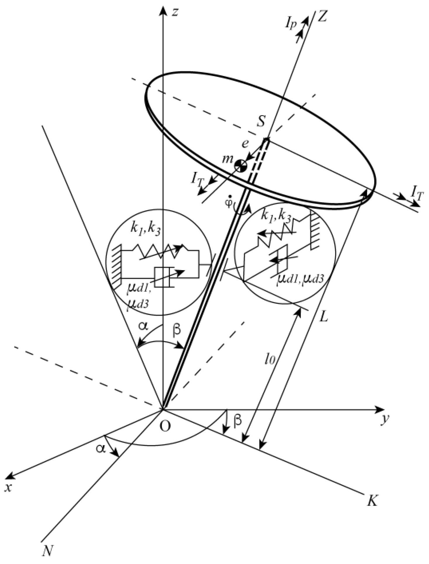
2.2. Equations of Motion and Their Solutions

An ideal model of a rotor is considered, the structural diagram of which is shown in Figure 1. The shaft with length L is installed vertically by means of the lower hinged and upper elastic support at a distance of l 0 . At the free end of the shaft, the disk is fixed, which has a mass m , a polar moment of inertia I p , and a transverse moment of inertia I T , the same for any direction. The speed of rotation w of the shaft is such that the rotor can be viewed as a gyroscope, the fixed point of which is the lower shaft support. The position of the geometric center of the disk S is determined by the coordinates x, y in a fixed coordinate system Oxyz, and the position of the shaft and rotor as a whole in space by the Euler angles α , β and the angle of rotation φ . The angles are small, and the movement of the rotor in the direction of the coordinate axis z is neglected. Next, we denote the coordinates of the center of mass m of the disk through x m and y m , respectively. It was assumed that the linear eccentricity e lies on the N axis of the ONKZ coordinate system. The deviations in the rotor axis were restricted to small values.
Expressing the projections of the angular velocity of the rotor in the coordinate axes of the ONKZ system, the coordinates of the center of mass of the disk and the coordinates of the upper support through the angular coordinates α , β and φ , finding expressions for the kinetic energy, potential energy of the rotor, the Rayleigh function and the projections of the moments of forces acting on the system, substituting them into the Lagrange equations of the second kind (Appendix A) obtain the equations of motion of the rotor in the form:
( I T + m L 2 ) α ¨ + I P ω β ˙ + μ d 1 α ˙ + μ d 3 α ˙ 3 + ( k 1 l 0 2 G L ) α + k 3 l 0 4 α 3 = ( m e ω 2 L + G e ) cos ω t , ( I T + m L 2 ) β ¨ I P ω α ˙ + μ d 1 β ˙ + μ d 3 β ˙ 3 + ( k 1 l 0 2 G L ) β + k 3 l 0 4 β 3 = ( m e ω 2 L + G e ) sin ω t .
On the right-hand part of the system of Equation (1), perturbations containing φ ¨ were discarded, because in the region close to the resonance velocity φ ¨ ω 2 , and perturbations having a parameter I P (in what follows, assuming that I P I T ) and values of the second and higher orders of smallness with respect to α ,   β , their derivatives, and their combinations. The indicated disturbances are small in comparison with disturbances, the amplitudes of which are proportional ω 2 .
Let us introduce the following dimensionless parameters:
e ¯ = e / L ;   l = l 0 / L ; t ¯ = t ω 0 ; Ω = ω / ω 0 ; I ¯ p = I p / ( m L 2 ) ; I ¯ T = I T / ( m L 2 ) ; K ¯ 1 = k 1 / ( m ω 0 2 ) ; K ¯ 3 = k 3 l 0 4 / ( m L 2 ω 0 2 ) ; G ¯ = G / ( m L ω 0 2 ) ; μ ¯ 1 = μ d 1 / ( m L 2 ω 0 ) ;   μ ¯ 3 = μ d 3 ω 0 / ( m L 2 ) ,
where
ω 0 = k 1 l 0 2 G L m L 2 ( I p I T )
is the natural frequency of the rotor system (1). Using (2), we obtain the equations of motion (1) in a compact dimensionless form:
( 1 + I ¯ T ) α + I ¯ p Ω β + μ ¯ 1 α + μ ¯ 3 α 3 + ( K ¯ 1 l 2 G ¯ ) α + K ¯ 3 α 3 = e ¯ ( Ω 2 + G ¯ ) cos Ω t ¯ , ( 1 + I ¯ T ) β I ¯ p Ω α + μ ¯ 1 β + μ ¯ 3 β 3 + ( K ¯ 1 l 2 G ¯ ) β + K ¯ 3 β 3 = e ¯ ( Ω 2 + G ¯ ) sin Ω t ¯ .
Here, prime denotes the derivative with respect to dimensionless time t ¯ .
After introduction of the designation of the dimensionless natural frequency of the linear rotor system at I ¯ T I ¯ p .
K ¯ 1 l 2 G ¯ 1 + I ¯ T = ω n ,
and the following designations for the dimensionless dynamic parameters of the oscillatory system
μ ¯ 1 1 + I ¯ T = μ 1 , μ ¯ 3 1 + I ¯ T = μ 3 , K ¯ 3 ( 1 + I ¯ T ) = K 3 , I ¯ P 1 + I ¯ T = I P 1 , e ¯ 1 + I ¯ T = e r
the equations of motion (4) can be given the following form
α + I P 1 Ω β + μ 1 α + μ 3 α 3 + ω n 2 α + K 3 α 3 = e r ( Ω 2 + G ¯ ) cos Ω t ¯ , β I P 1 Ω α + μ 1 β + μ 3 β 3 + ω n 2 β + K 3 β 3 = e r ( Ω 2 + G ¯ ) sin Ω t ¯ .
Consider a rotor system that is nearly linear. For this system, the equations of motion (7) are solved using an asymptotic method, for example, by the varying amplitude method (VAM) [38].
To apply the method of slowly varying amplitudes, the following restrictions were considered. The projections of the moments of the damping forces μ 1 α , μ 1 β and μ 3 α 3 ,   μ 3 β 3 , as well as the moment of the cubic component of the restoring force K 3 α 3 , K 3 β 3 , the moments of the inertial force of the mass imbalance, and the gravity force e r ( Ω 2 + G ¯ ) cos Ω t ¯ , e r ( Ω 2 + G ¯ ) sin Ω t ¯ are considered small in comparison to other moments of forces acting on the system. Assuming that I ¯ p I ¯ T the projections of the moment of the passive gyroscopic force, I P 1 Ω α and I P 1 Ω β , can also be considered small. Besides, considering a spinning rotor, Ω 2 G ¯ , and motion in the resonance range, where the frequency of free oscillations ω n is close to the frequency of forced oscillations Ω , ξ = ε ξ 1 = Ω ω n ω n is a small parameter, and ε 1 .
Equation (7), at small values of the quantity ξ and the accepted constraints of the problem, takes the following form:
α + Ω 2 α = e r Ω 2 cos Ω t ¯ I P 1 Ω β μ 1 α μ 3 α 3 ω n 2 α K 3 α 3 + 2 ξ α , β + Ω 2 β = e r Ω 2 sin Ω t ¯ + I P 1 Ω α μ 1 β μ 3 β 3 ω n 2 β K 3 β 3 + 2 ξ β .
Equation (8) is a system of second-order nonlinear ordinary differential equations with respect to   α , β .
To investigate the forced fundamental resonant oscillations, solutions (8) are analyzed at the frequency of the exciting moment:
α = A ( t ¯ ) cos [ Ω t ¯ + θ ( t ¯ ) ] ,
β = A ( t ¯ ) sin [ Ω t ¯ + θ ( t ¯ ) ] .
Here, A ( t ¯ ) is the slowly varying amplitude, θ ( t ¯ ) is the phase shift of the oscillations relative to the forced harmonic moment.
Using the method of varying amplitude relative to the angular coordinates (9) and (10), conditions imposed (A11) and (A12) on variables A   and θ (Appendix B), we obtain a system of abbreviated equations:
A = 1 2 π 0 2 π / Ω [ e r Ω 2 cos Ω t ¯ + ( 2 ξ Ω I P 1 Ω 2 ) A cos ( Ω t ¯ + θ ) + μ 1 Ω A sin ( Ω t ¯ + θ ) + μ 3 Ω 3 A 3 sin 3 ( Ω t ¯ + θ ) K 3 A 3 cos 3 ( Ω t ¯ + θ ) ] sin ( Ω t ¯ + θ ) d t ¯
A θ = 1 2 π 0 2 π / Ω [ e r Ω 2 cos Ω t ¯ + ( 2 ξ Ω I P 1 Ω 2 ) A cos ( Ω t ¯ + θ ) + μ 1 Ω A sin ( Ω t ¯ + θ ) + μ 3 Ω 3 A 3 sin 3 ( Ω t ¯ + θ ) K 3 A 3 cos 3 ( Ω t ¯ + θ ) ] cos ( Ω t ¯ + θ ) d t ¯
After integrating Equations (11) and (12), we derive the system of equations for transient oscillations of the rotor:
A = 1 2 e r Ω sin θ 1 2 μ 1 A 3 8 μ 3 Ω 2 A 3 ,
A θ = 1 2 e r Ω cos θ 1 2 ( 2 ξ I P 1 Ω ) A + 3 K 3 8 Ω A 3 .  
Equations (13) and (14) can also be obtained using Equations (10), (A8) and (A12), along with the method of slowly varying amplitude applied to the second equation of the system (8).
Stationary modes of motion are determined under the conditions A ˙ = 0 and θ ˙ = 0 by equations
1 2 e r Ω sin θ 0 = 1 2 μ 1 A 0 + 3 8 μ 3 Ω 2 A 0 3
1 2 e r Ω cos θ 0 = 1 2 ( 2 ξ I P 1 Ω ) A 0 + 3 K 3 8 Ω A 0 3 .
Equations (15) and (16) with the use of the designation for the frequency detuning ξ * = ξ 1 2 I P 1 Ω with a correction taking into account the passive gyroscopic torque gives the expression for determining the amplitude of stationary oscillations
{ ( μ 1 Ω + 3 4 μ 3 Ω 3 A 0 2 ) 2 + ( 3 4 K 3 A 0 2 2 ξ * Ω ) 2 } A 0 2 = ( e r Ω 2 ) 2 .

2.3. Nonlinear Frequency Characteristics

For calculations, the general parameters of the system were selected in accordance with various design parameters of the centrifuge used in [10] for experimental studies, and have the following dimensionless values: er = 0.0346, ωn ≈ 1, IP1 = 0.021 ( I ¯ P = 0.026 ,     I ¯ T = 0.213 ). The values of the parameters, K 3 ,   μ 1 ,   μ 3 and Ω are selected in the course of numerical experiment taking into account the remaining known design parameters necessary to create effective vibration isolation for the gyroscopic rotor. Figure 2 and Figure 3 show the resonance curves on the plane ( A 0 ,   ξ * ) for different values of the linear damping coefficient μ 1 = 0.01 ,   0.02 ,   0.03 ,   0.04 at μ 3 = 0 , K3 = 0.05 and the non-linear cubic damping coefficient μ 3 = 0.010 ,   0.020 ,   0.043 ,   0.060 at μ 1 = 0.01 , K3 = 0.1, respectively. It is clearly seen that when μ 1 is equal to or greater than a certain value μ 1 * = 0.03 , and μ 3 equal to or greater than a certain value μ 3 * = 0.043 , the resonance curves resemble those of a linear rotor system with linear damping.
If μ 1 is equal to or less than a certain value μ 1 * = 0.03 , and μ 3 is equal to or less than a certain value μ 3 * = 0.043 , the maximum of the resonance curves is shifted towards higher speeds of the shaft rotation, given that the natural frequency of the nonlinear rotor system increases with increasing amplitude of oscillations (rigid material of an elastic support, K 3 > 0 ). If, with an increase in the amplitude of oscillations, the natural frequency of the nonlinear rotor system decreases (soft material of an elastic support, K 3 < 0 ), then the maximum of the resonance curves shifts toward lower speeds of the shaft rotation. Suppression of the vibrational amplitude peak is clearly visible in the resonant region under the combined influence of the linear and nonlinear cubic damping of an elastic support.
The stability analysis of various branches of the resonance curves in Figure 4 and Figure 5 shows that the middle branch, marked with a dotted line from point 1 to point 2, is unstable.

2.4. Analysis of Solutions of Motion Equations

When changing the disalignment, moving along the curve from left to right, we observe the following: At ξ * = 0 , the exact resonance for the linear approximation, the amplitude of the oscillations is far from the maximum. The maximum amplitude A 0 m was observed for a certain value of disalignment, ξ * > 0 . With a further increase in the disalignment and when ξ * = ξ 1 * , the amplitude decreases, and the jump of oscillations to a much smaller amplitude occurs. In the reverse course of the disalignment, a jump occurs at ξ * = ξ 2 * < ξ 1 * , and the amplitude increases sharply. The values of the amplitudes A 01 and A 02 , at which jumps occur, are determined from the equation
d A 0 d ξ * =
(at points A 01 and A 02 , vertically tangent to the resonance curve).
To determine ξ 1 * , ξ 2 * ,   A 01 , and A 02 are differentiated by ξ * in Equation (17), taking into account that ξ * only depends on A 0 :
d A 0 d ξ * = 2 Ω ( 3 4 K 3 A 0 2 2 ξ * Ω ) A 0 ( μ 1 Ω + 3 4 μ 3 Ω 3 A 0 2 ) ( μ 1 Ω + 9 4 μ 3 Ω 3 A 0 2 ) + ( 3 4 K 3 A 0 2 2 ξ * Ω ) ( 9 4 K 3 A 0 2 2 ξ * Ω ) .
The values ξ 1 * and ξ 2 * , A 01   and   A 02 can be found from the simultaneous solution of equation
( μ 1 Ω + 3 4 μ 3 Ω 3 A 0 2 ) ( μ 1 Ω + 9 4 μ 3 Ω 3 A 0 2 ) + ( 3 4 K 3 A 0 2 2 ξ * Ω ) ( 9 4 K 3 A 0 2 2 ξ * Ω ) = 0
and Equation (17) for the resonance curve. The roots ξ 1 * and ξ 2 * in Equation (20) must satisfy the conditions of a positive discriminant for 9 K 3 2 27 μ 3 2 Ω 6 > 0 .
The values of the damping coefficients μ 1 * and μ 3 * at which hysteresis appears on the resonance curves or hopping effects are completely eliminated are determined from the condition of equality of the roots (20)
ξ 1 * = ξ 2 * = 3 K 3 A 0 2 4 Ω ,
i.e., vanishing of its discriminant
( 9 K 3 2 27 μ 3 2 Ω 6 ) A 0 4 48 μ 1 μ 3 Ω 4 A 0 2 16 μ 1 2 Ω 2 = 0
Here, the value K 3 included in Equation (22) is squared, and therefore, this equation is feasible in the case K 3 > 0 and in the case K 3 < 0 .
At μ 3 = 0 out of (22) it follows:
A 0 2 = 4 μ 1 Ω 3 K 3 .
Substituting (23) into (21), we obtain:
ξ 1 * = ξ 2 * = μ 1 * .
Substituting (23) and (24) into (17), we find:
μ 1 * = 1 2 3 e r 2 ( ± K 3 ) Ω . 3
At μ 1 = 0 out of (22) we find:
μ 3 * = ± K 3 3 Ω 3 .
In expressions (25) and (26), the “plus” sign corresponds to the rigid elasticity characteristic, and the “minus” sign corresponds to the soft elasticity characteristic of the support material.
From (25) and (26), it can be concluded that as the values of e r and K 3 increase, the amount of damping for the elastic support material required to eliminate the hopping effect increases.
For a given μ 3 = 0 ,   e r = 0.0346 , and K 3 = 0.05 , the coefficient of linear damping of the support material is μ 1 * = 0.0282 0.03 , and with μ 1 = 0 ,   e r = 0.0346 , and K 3 = 0.1 , the coefficient of nonlinear cubic damping of the support material is μ 3 * = 0.0577 .
By equating expression (19) for the derivative to d A 0 / d ξ * zero, we find the value of the maximum vibration amplitude:
A 0 m 2 = 8 ξ * Ω 3 K 3
Then from (17), it follows:
0.75 μ 3 Ω 2 A 0 m 3 + μ 1 A 0 m e r Ω = 0
and
A 0 m = e r 1.5 μ 3 Ω + ( μ 1 2.25 μ 3 Ω 2 ) 3 + ( e r 1.5 μ 3 Ω ) 2 3 + e r 1.5 μ 3 Ω ( μ 1 2.25 μ 3 Ω 2 ) 3 + ( e r 1.5 μ 3 Ω ) 2 3 .
At μ 3 = 0 in (27), we get
A 0 m = e r Ω μ 1 ,
and at μ 1 = 0 in (27), it follows
A 0 m = e r 0.75 μ 3 Ω 3 .
By analyzing Equations (29) and (30), we can say that the greater the eccentricity of the rotor mass, the greater the maximum amplitude, and to suppress the maximum amplitude, a significant damping of the elastic support material is required.
The responses of the gyroscopic rotor system in solving the equations of motion by different methods are evident in the oscillograms of the shaft rotation angle α = α ( t ¯ ) , shown in Figure 6. With K 3 = 0.05 , linear μ 1 = 0.04 (case a), and with K 3 = 0.1 , joint damping μ 3 = 0.043 , μ 1 = 0.01 (case b). The angular velocity of the shaft Ω = 0.7 and the other parameters of the rotor were previously given. Although the results show agreement, a slight difference in the maximum value of the responses is explained by the notion that in the VAM, the oscillation span is averaged, and when using the HBM, the main harmonic expansion of the solutions of the equations of motion for the same initial phase of oscillations was limited. Figure 6b shows a comparison of the effect of joint damping with that in Figure 6a.

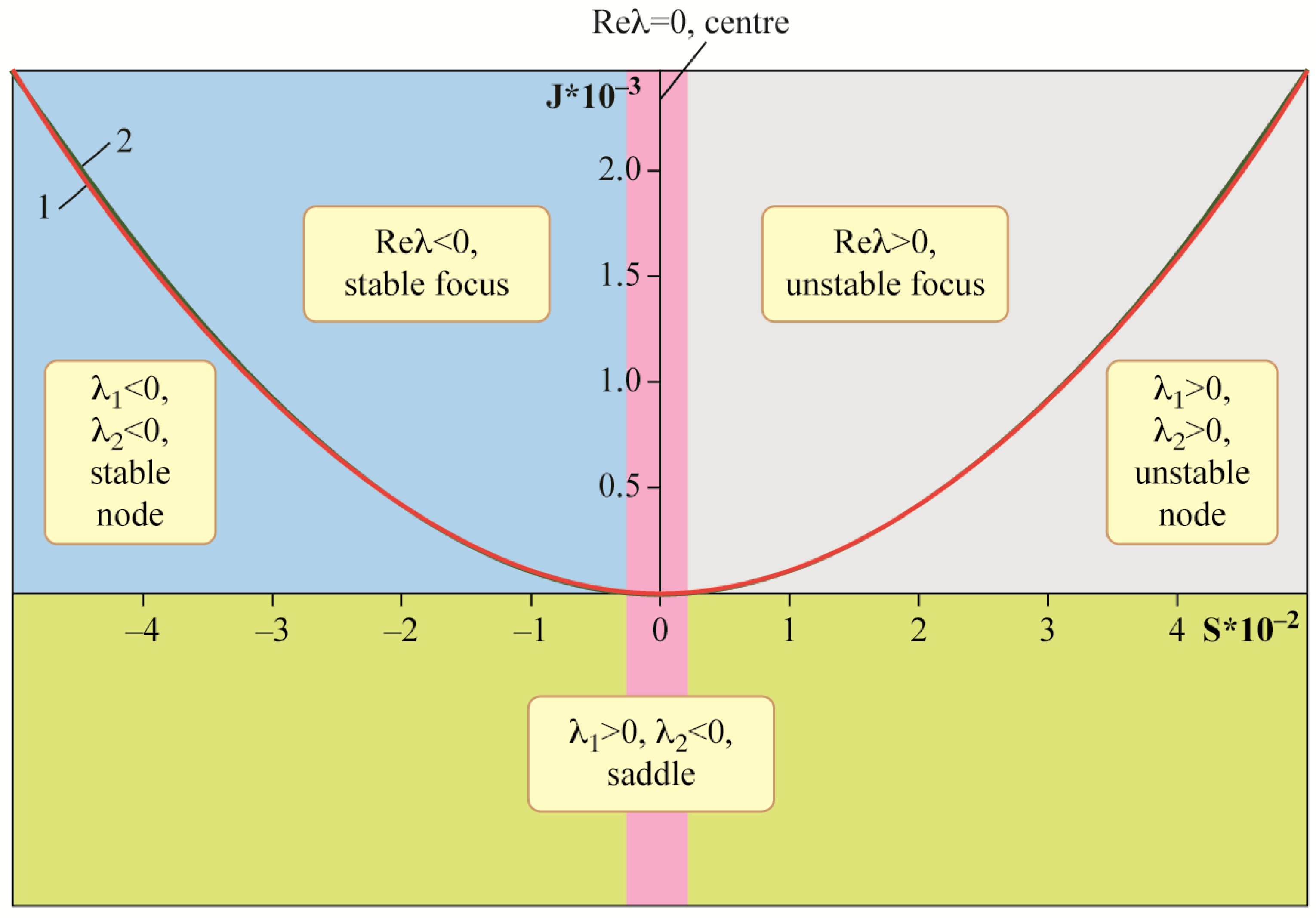
2.5. Stability of Stationary Motion

To consider the stability of the stationary motion of the rotor system, Equations (13) and (14) are reduced to the following form:
d A d t ¯ = Φ ( A ,   θ ) ,   d θ d t ¯ = Ψ ( A ,   θ ) ,
where
Φ ( A ,   θ ) = 1 2 e r Ω sin θ 1 2 μ 1 A 3 8 μ 3 Ω 2 A 3
and
Ψ ( A ,   θ ) = 1 2 A e r Ω cos θ ξ * + 3 K 3 8 Ω A 2
are smooth functions of variables A ,   θ .
In stationary motion, that is, at A = A 0 and θ = θ 0 , the right-hand sides of the system of Equation (31) vanish. We set small deviations from the equilibrium point η = A A 0 ,   ζ = θ θ 0 and expand the functions in a series Φ ( A ,   θ ) and Ψ ( A ,   θ ) in a small neighborhood A = A 0 of and θ = θ 0 , limiting ourselves to the first degrees for A and θ . Then, the system of Equation (31) can be written in the form:
η ˙ = ( Φ A ) 0   η + ( Φ θ ) 0   ζ ,
ζ ˙ = ( Ψ A ) 0   η + ( Ψ θ ) 0   ζ ,
where derivatives
( Φ A ) 0 = 1 2 μ 1 9 8 μ 3 A 0 2 , ( Φ θ ) 0 = 1 2 e r Ω cos θ 0 , ( Ψ A ) 0 = 1 2 A 0 2 e r Ω cos θ 0 + 3 4 Ω K 3 A 0 , ( Ψ θ ) 0 = 1 2 A e r Ω sin θ 0
was taken at the point of equilibrium. Specifying the solutions of this system of equations in the form η ~ e λ t ¯ ,   ζ ~ e λ t ¯ , to determine the characteristic exponent λ , we obtain the following equations:
[ ( Φ A ) 0 λ ] η + ( Φ θ ) 0   ζ = 0 ,
( Ψ A ) 0 η + [ ( Ψ θ ) 0 λ ] ζ = 0 ,
For a homogeneous system of equations to have a nontrivial solution, it is necessary to require the equality of its determinant to zero
| ( Φ A ) 0 λ ( Φ θ ) 0 ( Ψ A ) 0 η   ( Ψ θ ) 0 λ   | = 0
Hence,
λ 2 + ( 1 2 μ 1 + 9 8 μ 3 Ω 2 A 0 2 1 2 A 0 e r Ω sin θ 0 ) λ 1 2 A 0 e r Ω sin θ 0 ( 1 2 μ 1 + 9 8 μ 3 Ω 2 A 0 2 ) + 1 2 e r Ω cos θ 0 ( 1 2 A 0 2 e r Ω cos θ 0 + 3 4 Ω K 3 A 0 ) = 0
and
λ 1 , 2 = ( 1 2 μ 1 + 9 8 μ 3 Ω 2 A 0 2 1 2 A 0 e r Ω sin θ 0 ) ± 1 2 ( 1 2 μ 1 + 9 8 μ 3 Ω 2 A 0 2 + 1 2 A 0 e r Ω sin θ 0 ) 2 4 1 2 e r Ω cos θ 0 ( 1 2 A 0 2 e r Ω cos θ 0 + 3 4 Ω K 3 A 0 ) .
Taking into account (15) and (16), expression (40) can be written as
λ 1 , 2 = 1 2 ( μ 1 + 3 2 μ 3 Ω 2 A 0 2 ) ± 1 2 [ ξ * ( 3 K 3 4 Ω 3 8 K 3 2 Ω 2 + μ 3 2 ) A 0 2 ] [ ξ * ( 3 K 3 4 Ω + 3 8 K 3 2 Ω 2 + μ 3 2 ) A 0 2 ] .
The roots of the characteristic equation determine the stability or instability of the equilibrium state. It can be seen from (41) that at ξ * < ( 3 K 3 4 Ω 3 8 K 3 2 Ω 2 + μ 3 2 ) A 0 2 and ξ * > ( 3 K 3 4 Ω + 3 8 K 3 2 Ω 2 + μ 3 2 ) A 0 2 , the roots λ1,2 are complex, and the equilibrium state is a stable focus. At ( 3 K 3 4 Ω 3 8 K 3 2 Ω 2 + μ 3 2 ) A 0 2 < ξ * < ( 3 K 3 4 Ω + 3 8 K 3 2 Ω 2 + μ 3 2 ) A 0 2 , the roots are real. In this case, the root λ 2 is negative, so the state can be either a stable node or a saddle. A change in the nature of stability occurs for the positive root λ 1 , that is, at
[ ξ ( 3 K 3 4 Ω 3 8 K 3 2 Ω 2 + μ 3 2 ) A 0 2 ] [ ξ ( 3 K 3 4 Ω + 3 8 K 3 2 Ω 2 + μ 3 2 ) A 0 2 ] = ( μ 1 + 3 2 μ 3 Ω 2 A 0 2 ) 2

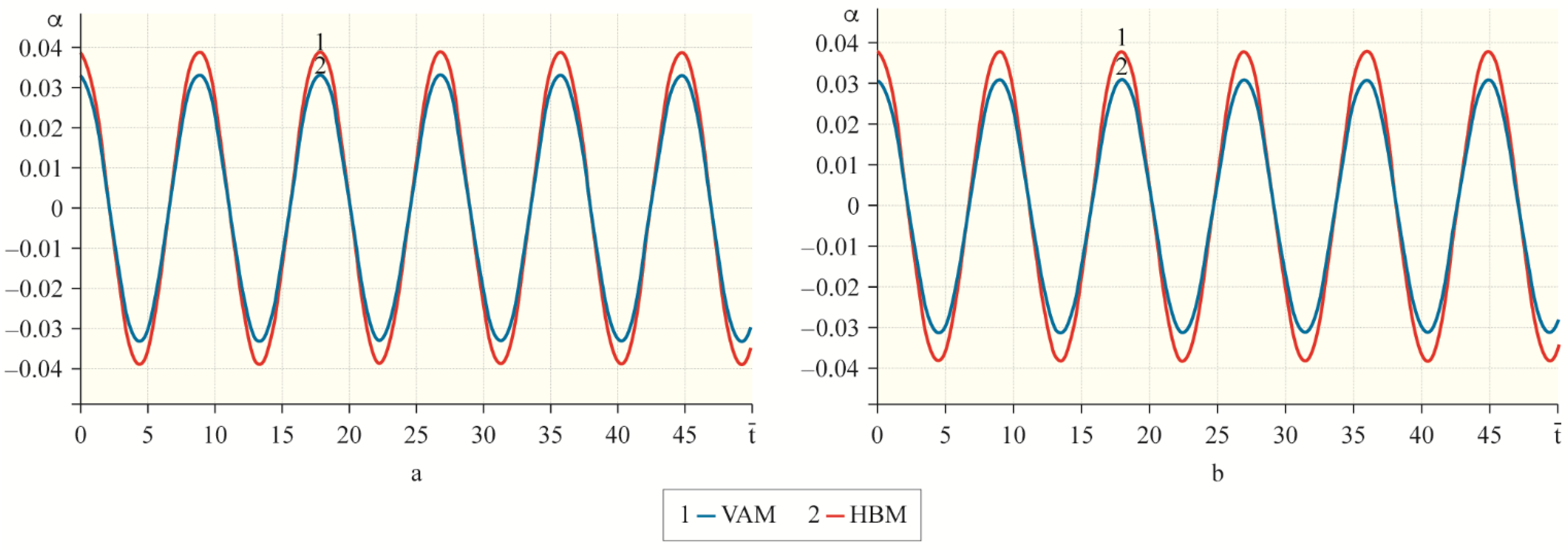
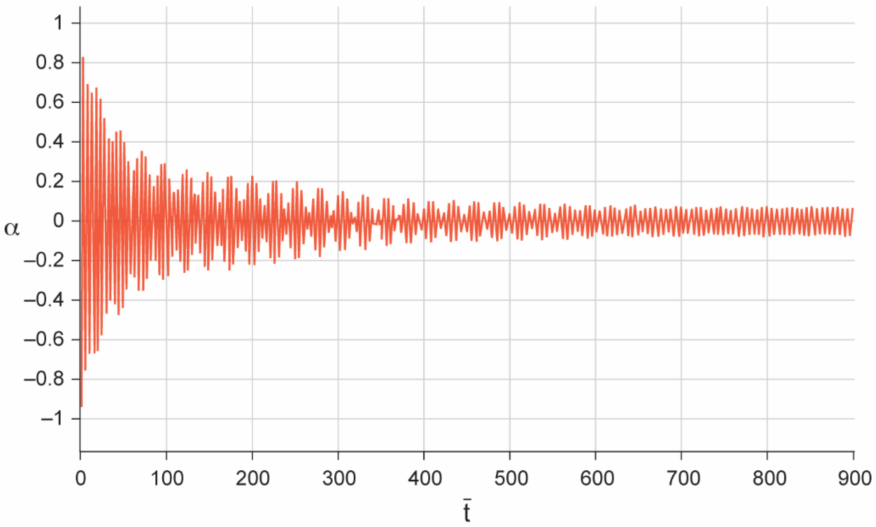
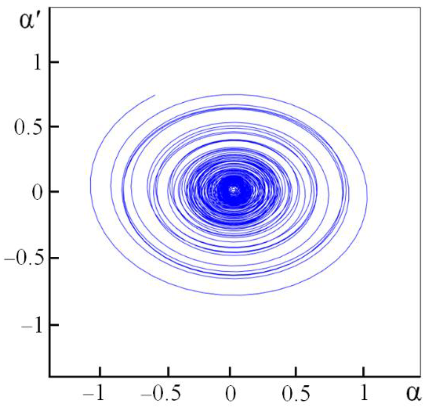
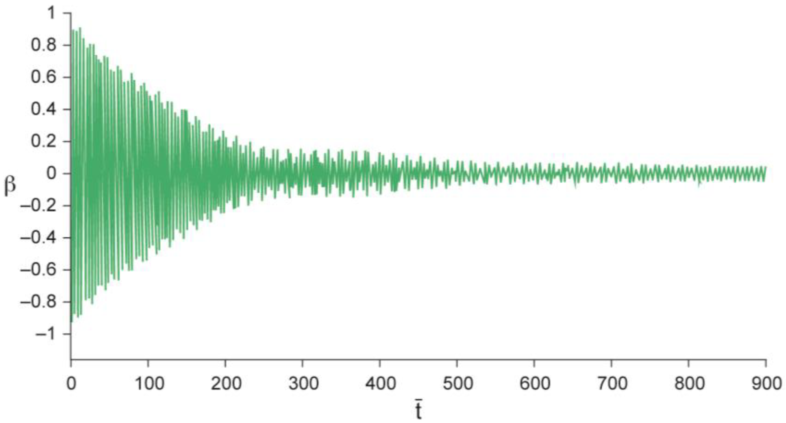
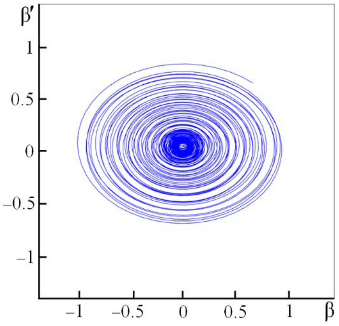
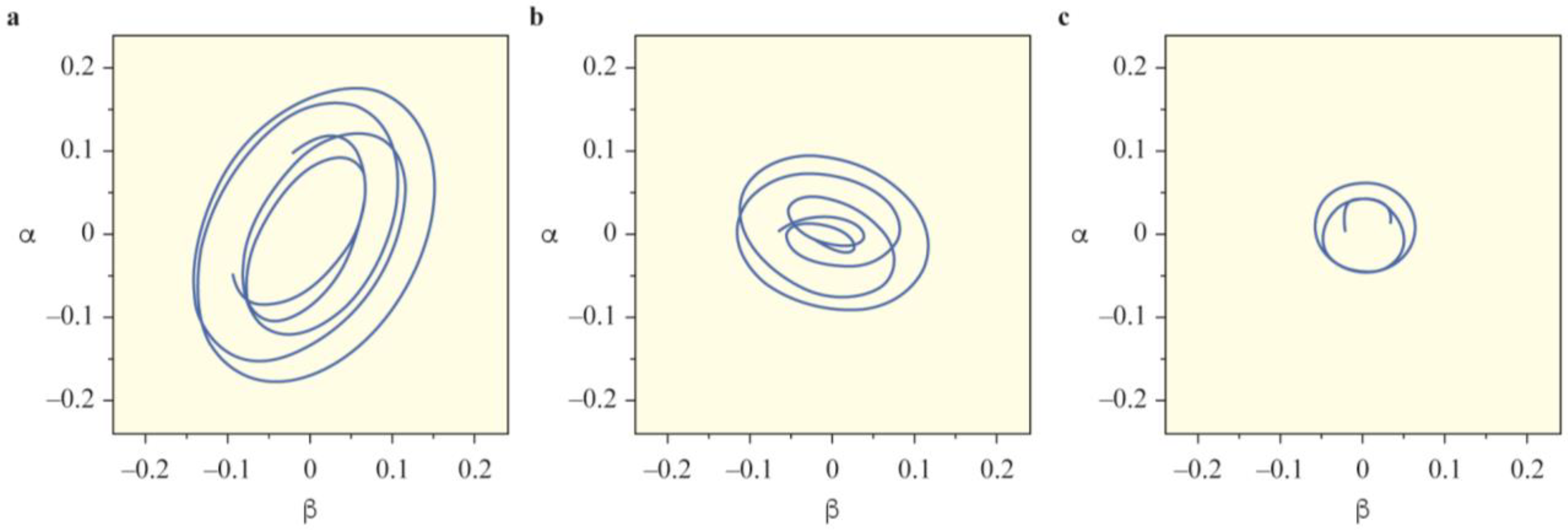
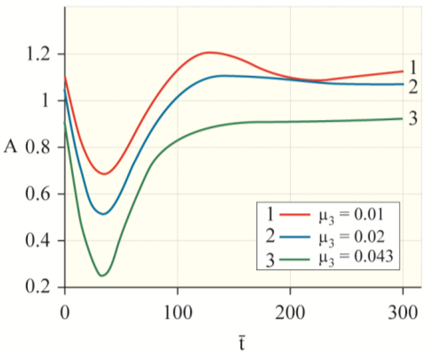
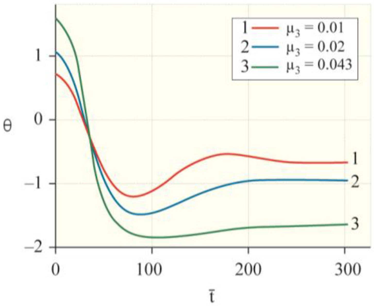
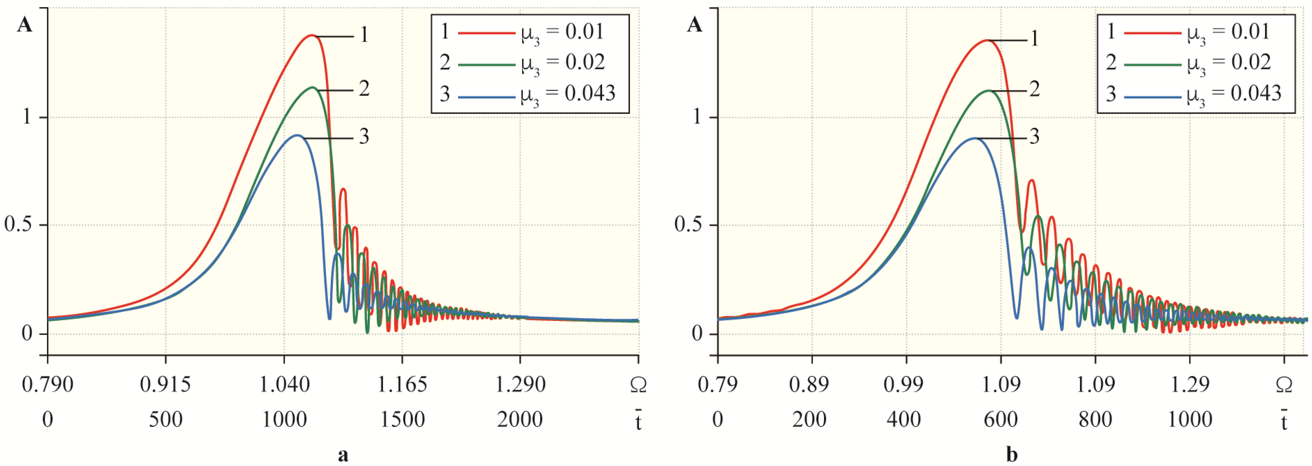
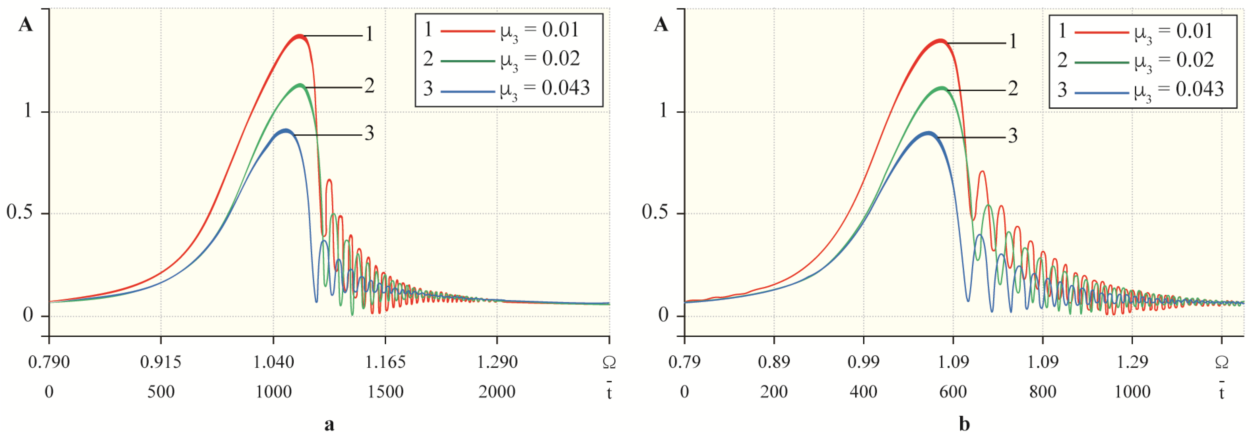
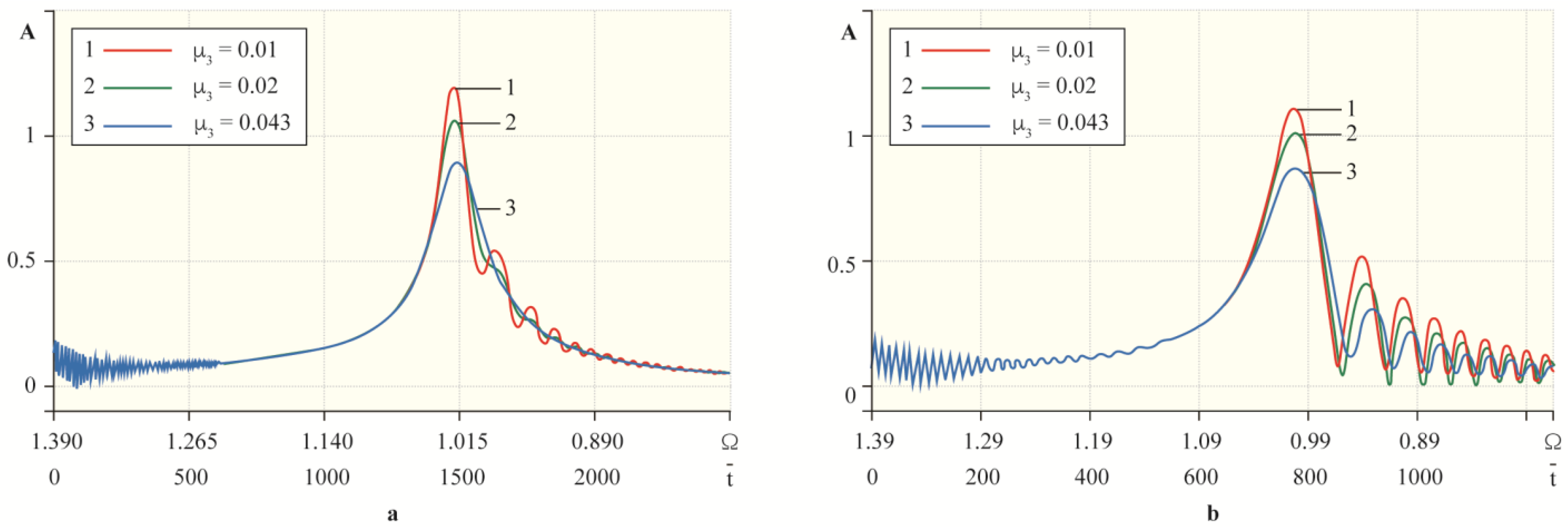
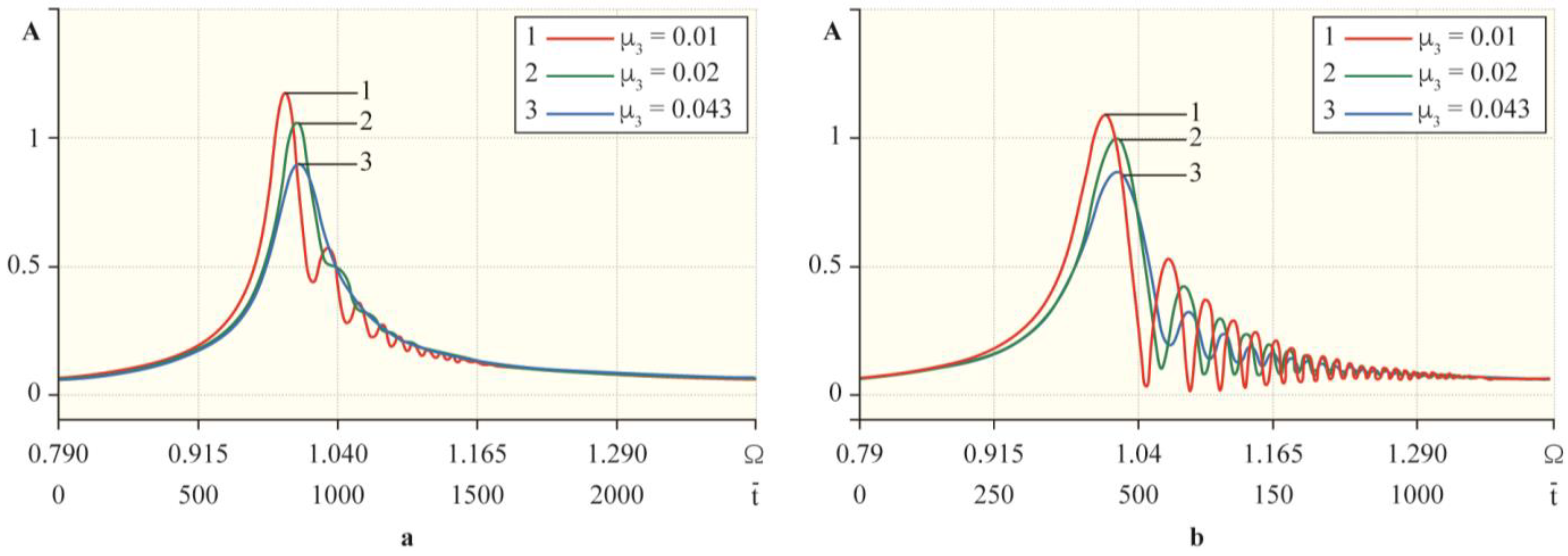
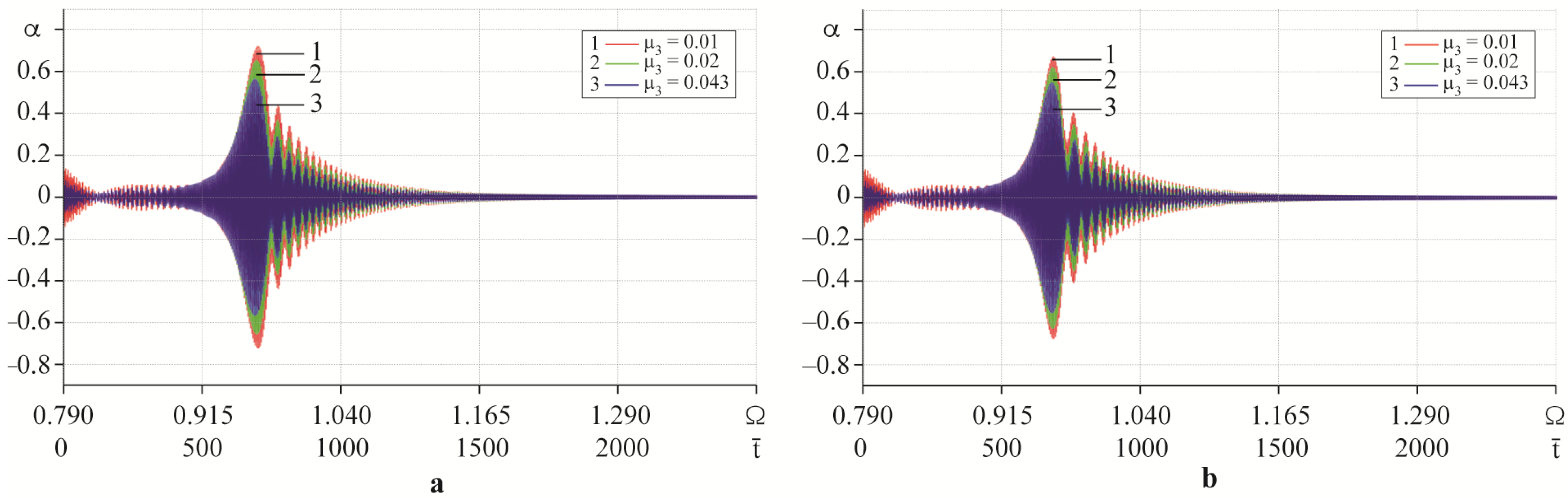
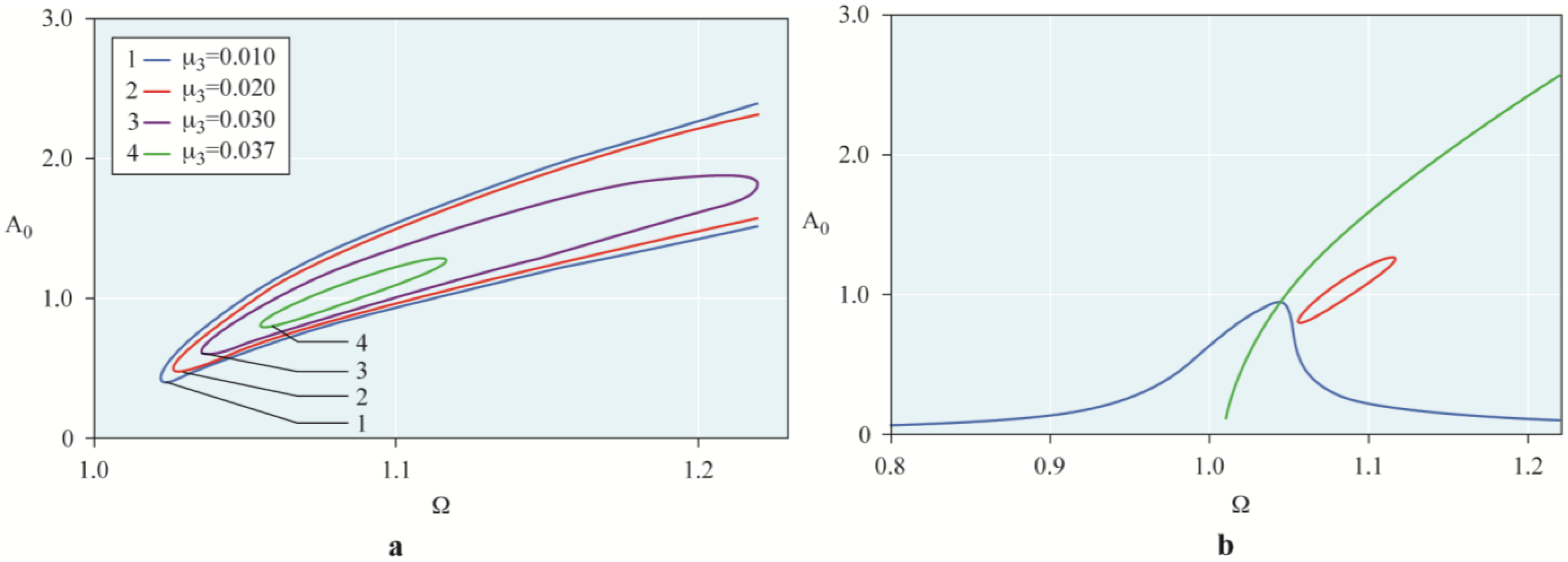
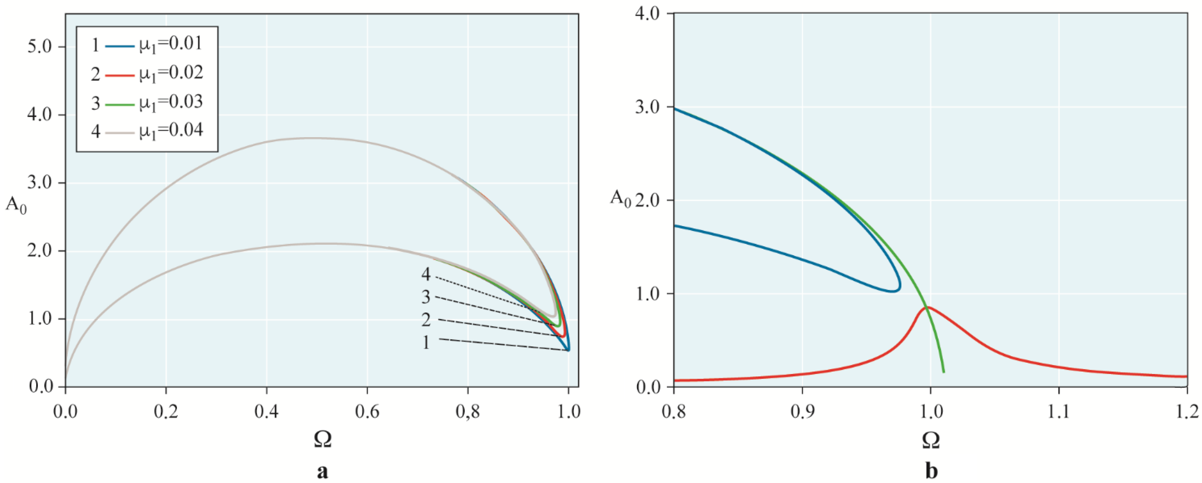
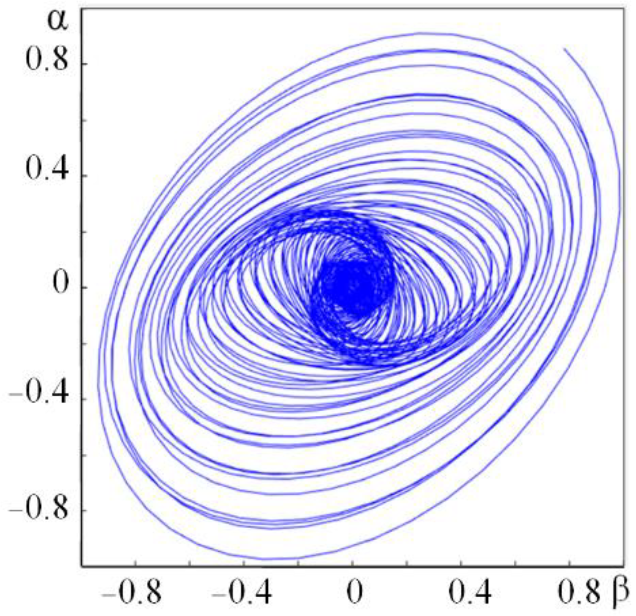
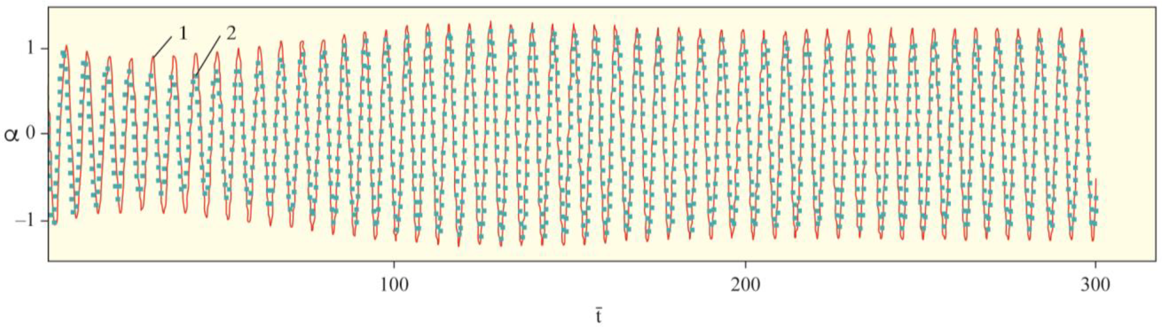
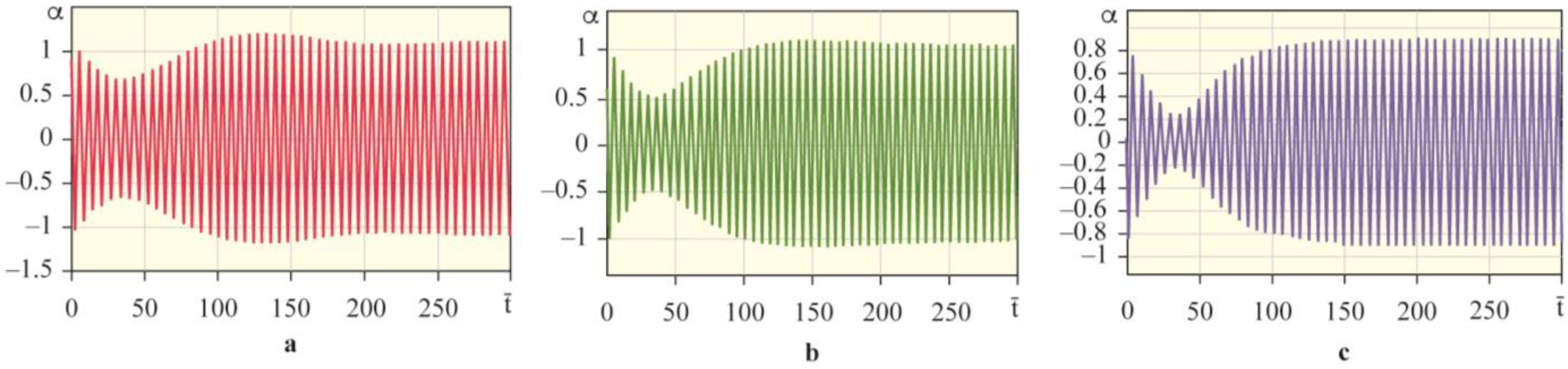
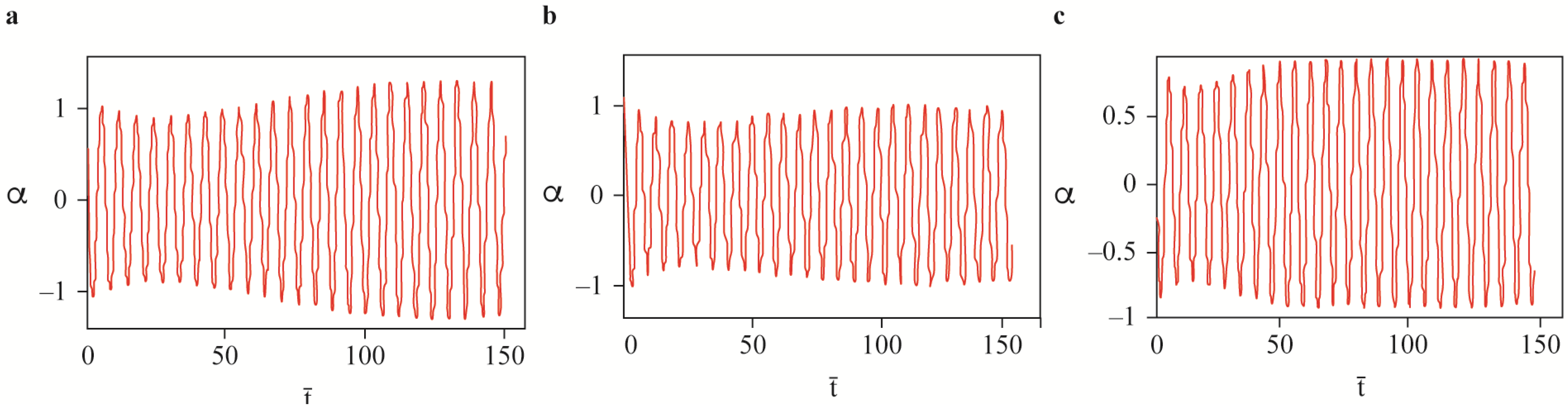
2.6. Non-Stationary Oscillations

To study the unsteady processes, Equations (13) and (14) are reduced to the following form:
d A / d t ¯ = ( 1 / 2 ) e r Ω sin θ ( 1 / 2 ) μ 1 A ( 3 / 8 ) μ 3 Ω 2 A 3 ,
d θ / d t ¯ = ( 2 / 2 A ) e r Ω cos θ ( Ω ω n I P 1 Ω / 2 ) + ( 3 K 3 / 8 Ω ) A 2 .
Equations (43) and (44) describe unsteady processes when their right-hand parts do not vanish, and when the processes develop in the resonance region. In such nonstationary processes, θ will be a slowly varying function of time t ¯ , which follows from the structure of Equations (43) and (44). Equation (43) describes the change in the amplitude of oscillations and the behavior of the envelope of the oscillatory process of angular coordinates α   and β ; Equation (44) describes the change in the initial phase θ of the oscillatory process.
Starting from some initial conditions, the rotor system tends towards the nearest stable stationary mode of motion.
At the initial conditions of the problem t ¯ = 0 ,   A = A ( 0 ) , θ = θ ( 0 ) , it is convenient to choose the values close to their resonance or maximum values in stationary modes of motion.
Functions A , θ are easily obtained by numerically integrating Equations (43) and (44).
In the future, to construct oscillograms of the oscillations of angular coordinates, Equations (9) and (10), Equations (A9) and (A10), taking into account (13) and (14), will be represented in the form:
α = A ( t ¯ ) cos [ Ω t ¯ + θ ( t ¯ ) ] ,
α = d A d t ¯ cos ( Ω t ¯ + θ ) A ( Ω + d θ d t ¯ ) sin ( Ω t ¯ + θ ) ,
β = A ( t ¯ ) sin [ Ω t ¯ + θ ( t ¯ ) ] ,
β = d A d t ¯ sin ( Ω t ¯ + θ ) + A ( Ω + d θ d t ¯ ) cos ( Ω t ¯ + θ ) .
To study the effect of nonlinear cubic damping of the elastic support material on the dynamics of the transient process, through the resonance region, following the method used in [39], the differential equations of the rotor motion in a compact dimensionless form are obtained:
α + Ω 2 ( τ ¯ ) α = e r Ω 2 ( τ ¯ ) cos φ I P 1 Ω ( τ ¯ ) β μ 1 α μ 3 α 3 ω n 2 α K 3 α 3 + 2 ξ α , β + Ω 2 ( τ ¯ ) β = e r Ω 2 ( τ ¯ ) sin φ + I P 1 Ω ( τ ¯ ) α μ 1 β μ 3 β 3 ω n 2 β K 3 β 3 + 2 ξ β ,
where Ω ( τ ¯ ) is the dimensionless speed of the shaft rotation, depending on τ ¯ = ε t ¯ “slow” dimensionless time [39]. Here, ε 1   is a small parameter.
In the oscillatory system, after a lapse of time, oscillations of one tone should be established, which in most cases occurs because of the presence of damping forces and external disturbances. The damping forces cause attenuation of the higher harmonics, and single-frequency oscillations of the basic tone with a frequency close to the forcing frequency are established in the system.
The single-frequency method allows us to consider both stationary oscillations and the process of the rotor transition through critical speeds under general conditions, causing the variability of the coefficients of the differential equations, in the presence of elastic supports with a non-linear characteristic of elasticity and nonlinear damping. Although the law of variation of the angular speed of the rotor can be obtained only on the basis of processing the results of experimental studies of acceleration and running down of the machine, to determine the general nature of the transient process, the single-frequency method solves the problem with the arbitrary law of variation of angular speed of the rotor. The only limitation that determines the applicability of this method is the requirement for a slow change in the angular velocity with respect to the natural frequency of the system under study.
Therefore, solutions (49) are in the form:
α = A ( t ¯ ) cos [ φ + θ ( t ¯ ) ] ,
β = A ( t ¯ ) sin [ φ + θ ( t ¯ ) ] .
Further, using the method of varying amplitude and proceeding as in Section 2, the equations of the transient process are obtained in the form
d A d t ¯ = [ e r Ω 2 ( τ ¯ ) cos φ + ( 2 ξ Ω ( τ ¯ ) I P 1 Ω 2 ( τ ¯ ) ) A cos ( φ + θ ) + μ 1 Ω ( τ ¯ ) A sin ( φ + θ ) + μ 3 Ω 3 ( τ ¯ ) A 3 sin 3 ( φ + θ ) K 3 A 3 cos 3 ( φ + θ ) ] sin ( φ + θ ) ,
A d θ d t ¯ = [ e r Ω 2 ( τ ¯ ) cos φ + ( 2 ξ Ω ( τ ¯ ) I P 1 Ω 2 ( τ ¯ ) ) A cos ( φ + θ ) + μ 1 Ω ( τ ¯ ) A sin ( φ + θ ) + μ 3 Ω 3 ( τ ¯ ) A 3 sin 3 ( φ + θ ) K 3 A 3 cos 3 ( φ + θ ) ] cos ( φ + θ ) .
After averaging Equations (52) and (53), the system of equations for the transient process of the rotor is obtained as follows:
d A d t ¯ = 1 2 e r Ω 2 ( τ ¯ ) sin θ 1 2 μ 1 Ω ( τ ¯ ) A 3 8 μ 3 Ω 3 ( τ ¯ ) A 3 ,
d θ d t ¯ = 1 2 A e r Ω 2 ( τ ¯ ) cos θ ( Ω ( τ ¯ ) ω n 1 2 I P 1 Ω ( τ ¯ ) ) Ω ( τ ¯ ) + 3 8 K 3 A 2 .

3. Results

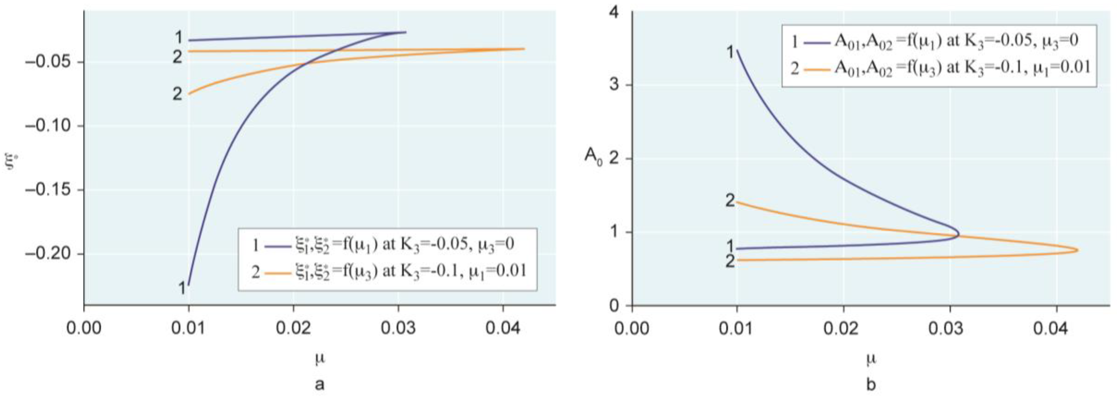
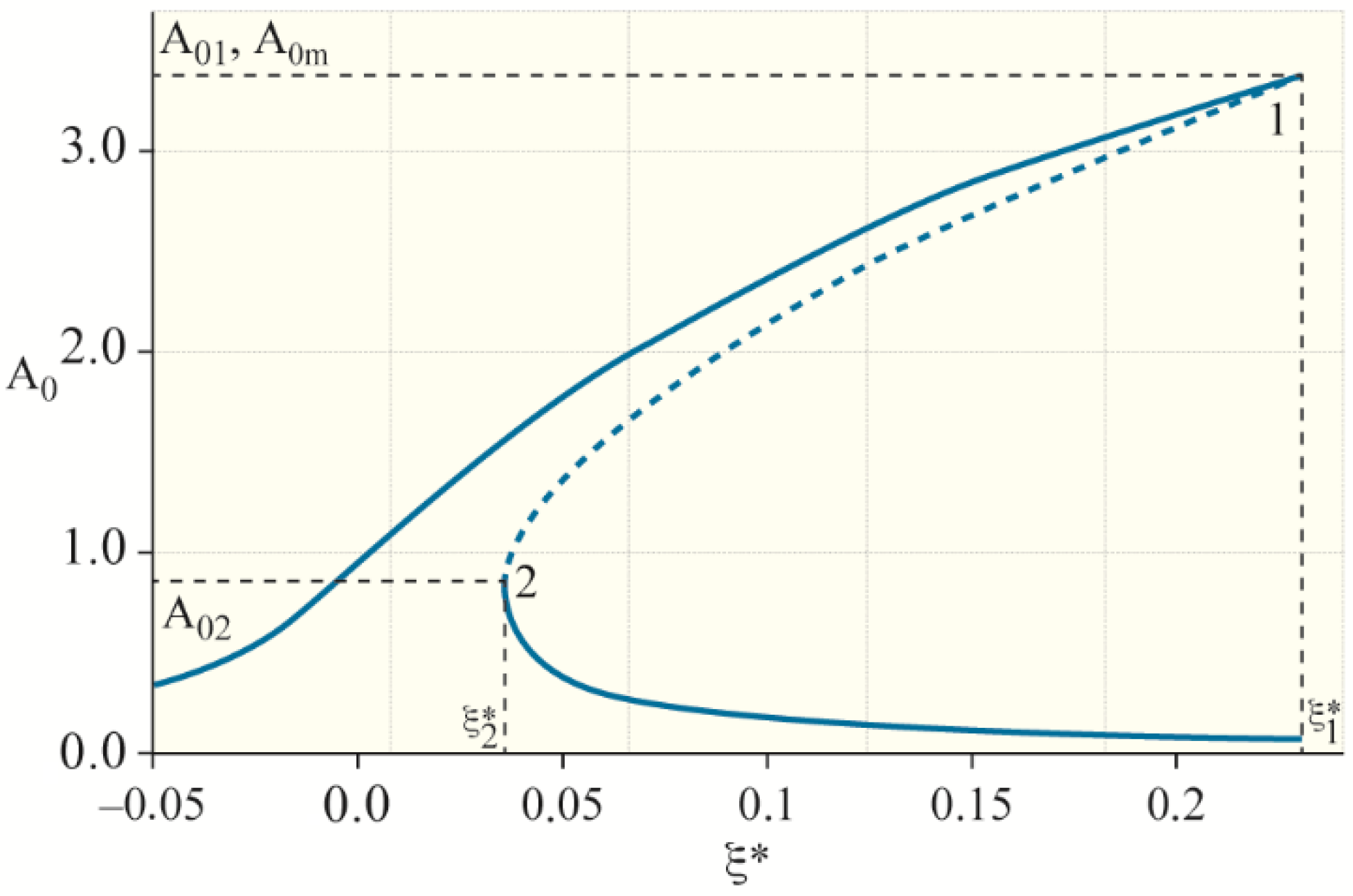
3.1. Stability of Stationary Motion

Now, we define the regions of the existence of singular points by introducing the characteristic Equation (51) into the form of the determinant of the Jacobi matrix [40]:
λ 2 S λ + J = 0 ,
where
S = ( μ 1 + 3 2 μ 3 Ω 2 A 0 2 )
and
J = ( μ 1 + 3 4 μ 3 Ω 2 A 0 2 ) ( μ 1 + 9 4 μ 3 Ω 2 A 0 2 ) + [ 3 K 3 4 Ω A 0 2 ( 2 I P 1 ) Ω + 2 ω n ] [ 9 K 3 4 Ω A 0 2 ( 2 I P 1 ) Ω + 2 ω n ] .
Solving Equation (56), we obtain two roots:
λ 1 = S / 2 + S 2 / 4 J   and   λ 2 = S / 2 S 2 / 4 J .
First, we assume that the discriminant of Equation (56) is positive. Second, both eigenvalues are real and distinct. If both eigenvalues are negative, then the perturbation decays over time and tends to zero, i.e., the rotary system approaches a special point referred to as a stable point. If at least one eigenvalue is greater than zero, then the corresponding component of the perturbation will increase, i.e., the rotor system will move away from a special point referred to as an unstable point.
Now, we let the discrimination of Equation (56) be negative. Both eigenvalues are complex, λ 1 , 2 = S / 2 ± i J S 2 / 4 , and one eigenvalue is obtained from the other eigenvalue by means of a complex conjugation operation. The time dependence of perturbations in this case is determined by an expression of the form e x p ( λ t ¯ ) cos ( λ t ¯ + φ ) , where λ is the real part of the eigenvalue and λ is the imaginary part of the eigenvalue. The singular point is stable if the real part λ < 0 is stable; if λ > 0 , the singular point is unstable.
The main interest is the typical situation to which the internal points of the regions shown in Figure 7 correspond. Special roles are played by the line S = 0 in the vicinity of which conservative systems “live” and the line J = 0 . We emphasize that for the singular point “center”, the damping coefficients μ 1 = 0 ,   μ 3 = 0 , and therefore, the axis   J is the dividing line of the regions of dissipative systems with positive damping and systems with negative damping. The position of the axis S is determined by the condition J = 0 , that is, the stability criterion:
( μ 1 + 3 4 μ 3 Ω 2 A 0 2 ) ( μ 1 + 9 4 μ 3 Ω 2 A 0 2 ) + [ 3 K 3 4 Ω A 0 2 ( 2 I P 1 ) Ω + 2 ω n ] [ 9 K 3 4 Ω A 0 2 ( 2 I P 1 ) Ω + 2 ω n ] = 0
Therefore, the axis S is the axis of the joint influence of linear and nonlinear cubic damping, because it is determined by Equation (57). On the other hand, the boundary of the regions of stability (stable focus and stable node) and regions of instability (saddle) are located in quadrants II and III, where μ 1 > 0 and μ 3 > 0 .
As shown in Figure 7, with joint linear and nonlinear cubic damping, the boundary lines of the regions of a stable (unstable) focus and a stable (unstable) node are slightly shifted to the center, which shows a weak nonlinearity of the gyroscopic rotor system under consideration.
Thus, the stability criterion (60) was allegedly obtained from the determinant of the matrix, which can also be obtained from the condition that the vertical tangent to the resonant curve corresponds to the stability boundary:
d Ω d A 0 F A 0 = 0 ,
where
F = { ( μ 1 Ω + 3 4 μ 3 Ω 3 A 0 2 ) 2 + [ 3 4 K 3 A 0 2 ( 2 I P 1 ) Ω 2 + 2 ω n Ω ] 2 } A 0 2 ( e r Ω 2 ) 2 = 0
This equation expresses the frequency response of an oscillatory gyroscopic rotary system.
The boundaries of the instability regions with different stiffness characteristics of the nonlinear elasticity of the support and different values of the damping coefficients are shown in Figure 8, Figure 9, Figure 10 and Figure 11. In the case of a rigid characteristic of the nonlinear elasticity of the support, an increase in the value of the linear damping coefficient shifts the left boundary of the instability region towards large oscillation amplitudes and shaft rotation speeds (Figure 8a).
After the jump effects are eliminated, the instability region becomes “disconnected” from the frequency response of the rotor system and will exist in part of the space behind the resonant rotation speed (Figure 8b). Simultaneously, the upper boundary practically coincides with the vertebral curve. The nonlinear cubic damping of the support material, with its linear damping, narrows the instability region from all its boundaries (Figure 9a). In the absence of jumping effects, the instability region can be located significantly below the vertebral curve. Its dimensions can significantly decrease depending on the magnitude of the joint damping (Figure 9b) and can even completely disappear, for example, at μ 3 = 0.03788 , μ 1 = 0.01 and other known data values. In the case of a soft characteristic of the nonlinear elasticity of the support, the nature of influence of linear damping and nonlinear cubic damping on the boundaries of the instability region is the same: an increase in the values of damping coefficients slightly shifts the near-resonant right boundary of the instability region towards lower shaft rotation speeds (Figure 10a and Figure 11a). The difference is that under the influence of nonlinear cubic damping, the ordinates of the lower and upper boundaries of the instability region are significantly shifted downwards. Figure 10b and Figure 11b show locations of the boundaries of the instability region relative to the frequency response with the vertebral curve. If Figure 10b is similar to Figure 8b, only with a difference in the deviation of the curves in the other direction, then in Figure 11b the resonant curve has a section of a nonlinear jump and is covered by a small section of the boundary lines of the instability region. Thus, if linear damping shifts the left boundary of the instability zone to the region of large amplitudes and speeds of rotation of the shaft, then joint linear and nonlinear cubic damping completely eliminate it.
In the solutions of the equations of motion (8) by the VAM, the averaged values of the maximum response of the system in the stationary mode exhibit minimal differences from the values of the real variable amplitude. Therefore, using this method, the display of the boundary of the stable motion of the system is more realistic.
In the non-uniqueness area, the resonance curve has three branches, the boundaries between which are determined from condition (18). Under this condition, Equation (20) takes the form (42). Consequently, the intermediate branch corresponds to an unstable equilibrium state, whereas the upper and lower branches correspond to stable states. In Figure 4 and Figure 5, the unstable branch is indicated by a prime.
The nonlinear rotor system demonstrated bistability in the area where hysteresis was realized. This corresponds to the presence in the phase space of two coexisting attractors, one of which corresponds to forced oscillations of small, and the other, of large amplitude. The occurrence of one or the other regime depends on the initial conditions. The trajectory comes to a specific attractor starting from the set of points in the phase space. For example, in Figure 12, Figure 13, Figure 14, Figure 15, Figure 16 and Figure 17, the oscillograms α = α ( t ¯ ) ,   β = β ( t ¯ ) and phase trajectories α = α ( α ) ,     β =   β ( β ) qualitatively show the transition process from the initial conditions: t ¯ = 0 :   Ω = 1.070 ,   A = 1.157 ,   θ = 0.7365 to an attractor with a smaller amplitude of stationary oscillations. In the transient process, damped beats were observed. The trajectories of the rotor shown in Figure 16 and Figure 17 show that in the transition process to the attractor, over time, the trajectories represent tilting, twisting clockwise, and decreasing elliptical spirals. The oscillograms of the deflection angle, the phase trajectory, and the trajectory of the rotor were constructed from the results of numerical solutions of the system of equations of the rotor motion (15), using the MathLab-Simulink package (R2021a (9.10.0.1602886) 64-bit (win61) 17 February 2021). In this case, the following values of the system parameters were used: er = 0.0346, ωn ≈ 1, IP1 = 0.021, K3 = 0.1, μ1 = 0.01, and μ3 = 0.01. An increase in the value of the nonlinear cubic damping coefficient to μ 3 * = 0.043 at μ 1 = 0.01 did not affect the behavior of the transient process.
Representation of the system behavior on the parameter planes ( ξ * ,   μ i ) and ( A 0 ,   μ i ) is useful, where i = 1, 3. Figure 18 and Figure 19 show the corresponding diagrams, where the abscissa shows the values of the linear and nonlinear cubic damping coefficients of the support and ordinates show the detuning (impact frequency) and vibration amplitude values, respectively. The bistability is limited by two lines with values of the disalignment ξ 1 *   and ξ 2 * , oscillation amplitudes A01 and A02, each of which corresponds to one of the roots of Equations (20) (or (42)) and (17). From Figure 18 and Figure 19, it can be seen that as the values of the linear damping coefficients or nonlinear cubic damping increase, the width of the bistability (hysteresis) area narrows, the distance between the jumps (attractors) decreases and the bordering lines intersect at the point ξ 1 * = ξ 2 * , A01 = A02 with the values μ 1 * and μ 3 * , respectively, the jumps (attractors) disappear. A change in the characteristic of the nonlinear elasticity of the support leads to a change in the coordinates of the boundary curves in the plane ( ξ * ,   μ ), and the nature of the dependencies   A 01 ,= f( μ i ), i = 1 ,   3 remains unchanged. The significant influence of the combined linear and nonlinear cubic damping of the support material is evident.
Let us consider an additional way to represent the behavior of a rotor system on the plane of its parameters. To do this, we consider the case where the angular speeds of rotation of the shaft Ω and ωn are close and, with the designation A *   = 3 K 3 A 0 2 4 μ 1 ω n ,   F = 3 K 3 ( e r ω n 2 ) 2 4 μ 1 3 ω n 3 , Ξ = 2 ξ * μ 1 ,   M 3 = μ 3 ω n 3 K 3 , reduce the equation of the resonance curve (17) to the following form:
A *   [ ( 1 + M 3 A * ) 2 + ( A * Ξ ) 2 ] = F .
Figure 20 shows diagrams at various values of the normalized nonlinear cubic damping coefficient M 3 of the support. In the diagrams, the horizontal line shows the normalized exposure frequency Ξ , and the ordinate is the normalized exposure amplitude F . This figure can be thought of as a set of partially overlapping sheets [40], each of which corresponds to one of the roots of Equation (63) at a certain value of μ 3 and given values e r ,   μ 1 = 0.01 ,   K 3 = 0.1 , and Ω ω n 1 . The overlapping area of the sheets is the bistability region bounded by two fold lines that converge at a point called the assemblage point [40]. The fold lines and the assemblage point are found using methods similar to those previously reported for ξ 1 * and ξ 2 * .
Moving along the plane of parameters along the horizontal line F = const, then the dependence of the vibration intensity on A *   the disalignment parameters Ξ will be given by the resonance curves of the family at various values of M 3 = 0.1 ,   0.2 (μ3 = 0.01, 0.02), as shown in Figure 3. If the considered horizontal line passes below the assemblage point, the dependence of the amplitude on the disalignment is unique. If it passes above the assemblage point, an area of ambiguity or hysteresis appears. It is limited by points Ξ 1 and Ξ 2   ( ξ 1 * and ξ 2 * ) , where the tangent to the resonance curve is vertical. These are the points where the line F = const intersects with the fold lines. The moment of the first appearance of the vertical tangent to the resonance curve at a point Ξ 1 = Ξ 2   ( ξ 1 * = ξ 2 * ) corresponds to the assemblage point. The graphs in Figure 20 also show the narrowing of the width of the bistability area as the coefficient of nonlinear cubic damping increases, and the expansion of this area as the amplitude of the moment of inertia of the mass imbalance increases with respect to the constant moments of the nonlinear elastic force and the linear damping force.

3.2. Non-Stationary Oscillations

When numerically integrating Equations (43), (44) and (7) in the resonant region, it was assumed that dimensionless nonlinear coefficient stiffness K = 0.1, and linear damping coefficient μ1 = 0.01.
The values of the parameters for the initial conditions are borrowed from the frequency characteristics of the stationary oscillation.
The initial conditions were chosen as: t ¯ = 0: (1) Ω = 1.0423, A = 1.10863, θ = 0.6611 at μ3 = 0.01; (2) Ω = 1.0423, A = 1.0631, θ = 0.9913 at μ3 = 0.02; (3) Ω = 1.0423, A = 0.9150, θ = 1.5080 at μ3 = 0.043.
The results of the integration of the system of Equations (43) and (44) in the resonance region, taking into account the initial conditions, are presented in the form of graphs A = A ( t ¯ ) and θ = θ ( t ¯ ) for different values of the nonlinear cubic damping coefficient μ3 = 0.01, 0.02, 0.043, and μ1 = 0.01, K3 = 0.1, as shown in Figure 21 and Figure 22. For all values of μ3, the parameters t ¯ A, θ begin to fluctuate over time; for example, the amplitude A first decreases, and then, having reached a minimum, it begins to increase, tending to the next stationary value, and to values larger than the initial values, since the initial values were less than the maximum values. The course of variation of the initial phase of oscillations θ over time t ¯ is similar; however, it tends towards values that are smaller than the initial values.
The reliability of the obtained results is achieved by comparing the results of the numerical solution of the system of differential equations of the rotor motion (8) with the results of the numerical solution of the differential equations of unsteady rotor oscillations (43) and (44). As shown in Figure 23, there is a considerable agreement between these results.
The oscillograms of α = α ( t ¯ ) rotor oscillations at different values of the nonlinear cubic damping coefficient μ3 = 0.01, 0.02, 0.043, and μ1 = 0.01, K3 = 0.1, by numerical solutions of the differential equations of the unsteady rotor oscillations (43) and (44), are shown in Figure 24. Similarly, Figure 25 shows the oscillograms according to the numerical solutions of the system of differential equations of the rotor motion (8). In both solutions, the effect of damping of the value of μ3 in the finite stationary values of the amplitude A, where its initial values tend during the non-stationary process, is clearly seen.
The MathLab and MathLab-Simulink packages (R2021a (9.10.0.1602886) 64-bit (win61) 17 February 2021) [41] were used for all numerical solutions of the equations of the nonstationary process and the system of equations of the rotor motion.
To illustrate the influence of the value of nonlinear cubic damping of the support on the development of the oscillatory process when passing through the resonant region, we consider the calculation of the unsteady mode of motion of the rotor system under the assumption that the speed of rotation of the shaft Ω is a “slowly” increasing parameter according to the law Ω = Ω 0 + ν t ¯ [39]. Transient Equations (52)–(55) were modeled using the Mathlab-Simulink package (R2021a (9.10.0.1602886) 64-bit (win61) 17 February 2021) [42,43].
The initial conditions are chosen at K 3 = 0.1, μ1 = 0.01 and t ¯ = 0 : (1) Ω = 0.81, A = 0.067, θ = −0.02521 at μ3 = 0.01; (2) Ω = 0.79, A = 0.06254, θ = −0.02297 at μ3 = 0.02; (3) Ω = 0.79, A = 0.0625381, θ = −0.0230614 at μ3 = 0.043.
Accepting the initial conditions at K 3 = −0.1, μ1 = 0.01 and t ¯ = 0 : (1) Ω = 0.80, A = 0.0664575, θ = −0.0240624 at μ3 = 0.01; (2) Ω = 0.79, A = 0.0626448, θ = −0.0230045 at μ3 = 0.02; (3) Ω = 0.79, A = 0.0626447, θ = −0.0231013 at μ3 = 0.043.
The abscissa axis has two scales: the Ω scale and the corresponding time scale t ¯ . The resonance curves of non-stationary rotor oscillations constructed on the results of modeling of Equations (52)–(55) are shown in Figure 26, Figure 27, Figure 28, Figure 29, Figure 30, Figure 31 and Figure 32. It can be clearly seen from all the graphs that an increase in the value of the non-linear cubic damping of the elastic support μ3 from 0.01 to 0.043 suppresses not only the maximum amplitude of the system response and its variation around the mean value, but also the vibration amplitude and its variation behind the rotation speed corresponding to the maximum amplitude. It shifts the shaft rotation speed Ω m corresponding to the maximum amplitude A m with a rigid nonlinear elastic characteristic ( K 3 > 0 ) of the support material downwards, and with a soft nonlinear elastic characteristic ( K 3 < 0 ) of the support material upwards, i.e., in both cases, the characteristics of the nonlinear stiffness Ω m of the support approach ω n . A similar effect was obtained with linear damping in [39]. From Figure 26, Figure 28 and Figure 29 it can be seen that with an increase in ν in absolute value from 0.00025 to 0.0005 during the machine acceleration, the maximum amplitude shifts towards high speeds of rotation, when braking the machine—towards low speeds of rotation and its value decreases [39].
A comparison of Figure 26 and Figure 27 and shows the identity of the results of solving the equations of the transient process before averaging (52) and (53) with the results of solving the equations of the transient process after averaging (54) and (55) over time, although Figure 27 shows a variation in the values of the amplitude of oscillations in time along the main curve around its mean values.
Changes in the nonlinear stiffness characteristics of an elastic support significantly affect the description of the resonance curves. The amplitude-frequency characteristics of the rotor during the transient process and the rigid characteristic of nonlinear elasticity of the support ( K 3 > 0 ) are shown in Figure 31, with the soft characteristic of nonlinear elasticity of ( K 3 < 0 ) the support—in Figure 32.
The values of the maximum amplitude and the corresponding rotational speed in the frequency response during the acceleration (Figure 31a and Figure 32a) and runout (Figure 31b and Figure 32b) of the rotary machine with   | ν | = 0.00025 , approximately determine the positions of the jumping effects. As the nonlinear cubic damping coefficient increases, the distance between these positions decreases, and its further increase can completely eliminate the jumping phenomena.
The difference in the values of the maximum amplitude, in the values of the corresponding shaft rotation speed, with increasing (Figure 31a and/or Figure 32a) and decreasing (Figure 31b and/or Figure 32b) shaft rotation speed is explained by jumping transitions with different values of these parameters, during the takeoff run and the rundown of the rotary machine. In the case of K > 0 and with   ν > 0 , the jump is performed from a large amplitude to a lower amplitude (Figure 31a), with ν < 0 from a lower amplitude to a higher amplitude (Figure 31b), and in the case of K 3 < 0 , vice versa (Figure 32a,b, respectively). This is usually observed in experimental studies during acceleration and deceleration of the machine [10]. With a rigid nonlinear elasticity characteristic of the support K 3 > 0 , jumps will be located in the area of the shaft rotation speed, where Ω > ω n (Figure 31), with a soft nonlinear support elasticity characteristic K 3 < 0 —In the range of the shaft rotation speed, where Ω < ω n (Figure 32).
To ensure the reliability of the process of transition through resonance, from Equation (17), setting the expression e Ω 2 equal to zero, due to the moment of inertia of the mass unbalance, and the damping coefficients, μ 1 and   μ 3 ,   the equation of the reference line of the resonance curve will be obtained:
Ω = ω n 2 I P 1 + ( ω n 2 I P 1 ) 2 + 3 K 3 A 2 4 ( 2 I P 1 ) .
At I P 1 2 and K 3 > 0 Ω > ω n , at K 3 < 0 Ω > ω n .
Assuming that, ν Ω 2 the maximum amplitudes and the corresponding rotational speeds of the resonance curves approximately satisfy Equation (64). The correspondence between the numerical (graphic) values of the peak amplitude A and the resonant velocity Ω for the given values of the linear damping coefficient μ1 and angular acceleration ν, and different values of the nonlinear stiffness coefficient K3 and the nonlinear cubic damping coefficient μ3 (Figure 26 and Figure 28), according to Formula (64), are given in Table 1.
To confirm the analytical study, Equation (8) was solved numerically. Figure 33 shows the numerical results obtained for passing through the resonance region with a rigid non-linear elastic characteristic of the support material and a “slowly” varying value of the angular velocity of rotation Ω . This figure shows that oscillations in the region of the maximum amplitude have a beat character, followed by damping beats, and the damping effect of μ3 is clearly visible in the resonant velocity region and beyond it. Damped beats occur due to the superposition of forced non-stationary oscillations and damped natural oscillations with frequencies closely matching in the vicinity of the resonance [39]. These results are consistent with the previous analytical results shown in Figure 26a and Figure 28a. The differences lie in the width of the region of clearly visible oscillations, the magnitude of the amplitude maximum, and the shift in the time instant of the amplitude maximum passage. Nevertheless, the basic behavior of the oscillatory process remains the same. No jumping effects were detected.

3.3. Methodology for Measuring and Identification of Damping Coefficients

Equations (25) and (26), using the notation for (2) and (6), can be rewritten in dimensional form. The formulas for determining the values of the coefficients of linear damping and nonlinear cubic damping of the support material, at which the jumping effects disappear, will have the form:
μ d 1 * = 1 2 3 ( e L ) 2 m L 2 l 0 4 k 3 ω 3   when   μ d 3 0
and
μ d 3 * = k 3 l 0 4 3 ω 3   when   μ d 1 0
In the case of combined linear and nonlinear cubic damping of the support material, the value μ d 3 * corresponding to the calculated values μ d 1 and k 3 is determined from Formula (29) in dimensional form:
[ ( μ d 1 ω + 3 4 μ d 3 ω 3 A 0 2 ) 2 + ( 3 4 k 3 A 0 2 2 Ξ * ω ) 2 ] A 0 2 = ( e m L 2 ω 2 / L ) 2 ,
where
Ξ * = ( m L 2 + I T ) [ ( 1 0.5 I P m L 2 + I T ) ω k 1 l 0 2 m g l m L 2 + I T ] ,
A 0 2 = 24 μ d 1 μ d 3 ω 4 9 l 0   8 k 3 2 27 μ d 3 2 ω 3 + ( 24 μ d 1 μ d 3 ω 4 9 l 0   8 k 3 2 27 μ d 3 2 ω 3 ) 2 + 16 μ d 1 2 ω 2 9 l 0   8 k 3 2 27 μ d 3 2 ω 3 .
Formula (69) is feasible only for the value μ d 3 * at μ d 1 0 . It should be noted that the expressions (65), (66) and (67) are applied only for small vibrations of the rotor shaft.
In Formulas (65), (66), and (67), the value of the nonlinear stiffness coefficient k 3 is determined from the equation of the reference curve [28] and from experimentally constructed frequency characteristics with the same value k 3 of the samples of the support material of the proposed gyroscopic rotor design:
k 3 = 8 ( m L 2 + I T ) 3 l 0 4 A 0 2 [ ω ( 1 0.5 I P m L 2 + I T ) k 1 l 0 2 m g l m L 2 + I T ] ω .
The vertebral curve is common for curves of frequency characteristics with the same value k 3 , including for a curve that satisfies condition (22).
First, we describe the methodology for determining the value μ d 3 * of the coefficient of nonlinear cubic damping at a relatively small value μ d 1 , which is the coefficient of linear damping of the support material. We construct resonant curves with the same value k 3 and several different values, but values μ d 3 near the value μ d 3 * are calculated by Formula (66) under the assumption that ω ( k 1 l 0 2 m g l ) / ( m L 2 + I T ) , according to the frequency response Equation (67). Analyzing the roots of Equation (67) for all values of the rotation speed of the entire range, from the constructed curves of the frequency response, we select the first curve, starting from the top, that has only one branch, which corresponds to one positive root of Equation (67) and a refined value μ d 3 * .
Next, we construct experimental resonance curves with an increasing and then decreasing parameter ω , with the same value k 3 and several values μ d 3 near the value μ d 3 * measured by a laser Doppler vibrometer [32,33]. Usually, the experimental curves of the frequency response of the forward and reverse strokes in the field of jumping effects do not coincide. We choose the resonant curves that coincide with the controlled acceleration and run-out of the rotary machine, with the value   μ d 3 * . By comparing the analytically constructed resonance curve that has the refined value μ d 3 * with the experimentally selected analogous curve, we identify the nonlinear cubic damping coefficient with the value μ d 3 * .
The value of the linear viscous damping coefficient μ d 1 * of a sample with a nonlinear stiffness coefficient k 3 and without nonlinear damping properties of the support material, determined by Formula (65), will be identified according to the abovementioned methodology. The approximate value μ d 3 * of the coefficient of nonlinear cubic damping of the support material, which simultaneously has linear damping ( μ d 1 0 ), is determined by Formula (67), taking into account (69) and the value k 3 obtained from the experimental resonance curves with the same value μ d 1 < μ d 1 * and different values μ d 3 , using Formula (70). Having constructed the curves of frequency characteristics according to Formula (67) μ d 3 for values near μ d 3 * and having analyzed the roots (67) of μ d 3 * , we specify the value and corresponding resonance curve. Next, the resonance curve with the specified value is compared to μ d 3 * with the corresponding experimental frequency response, and the value μ d 3 * is identified.
Thus, the methodology for determining and identifying the parameters k 3 ,   μ d 1 * , μ d 3 * and μ d 3 * at μ d 1 * 0 was described. The procedure for identifying these parameters of the support material and evaluating the values obtained in comparison with the results obtained by experimental and other methods require a separate study.
By measuring the parameters of the linear and nonlinear characteristics of a rubber rectangular plate according to the proposed methodology, it is possible to choose rubber plates for a support with the necessary geometric, nonlinear elastic, and damping characteristics. This finding suggests that based on the results of the above-mentioned research and patent search, it is possible to propose 3D models (Figure 34) and designs (Figure 35) of an elastic support and a centrifuge based on a vertical rigid gyroscopic rotor. Here, the results of experimental studies [10] on confirming the linear and nonlinear damping properties of the rubber support material were also taken into account. 3D modeling was carried out in the Solide Works environment [44]. The main difference between the centrifuge and its model proposed in [10] is the improved design of the elastic support. In [10], a whole corrugated rubber was used as a damping material around the shaft. In the design shown in Figure 34, rubber plates with the shape of a rectangular parallelepiped installed in six grooves of the support structure adjacent to the coupling are selected for this purpose. The shaft rotates freely on the bearing located in the coupling, which ensures the simplicity of the design, easy changeability of similar materials with other elastic and damping characteristics, and control of the number and location of rubber plates. Other differences include the replacement of electromagnetic motion and rotation speed sensors with more accurate laser sensors and the use of a computer to control and measure the necessary parameters.
In Figure 35, the centrifuge consists of a platform 1, a housing 2, a cylindrical container 3, a drive motor 4, rigidly placed inside the cylindrical casing 5. The cylindrical casing 5 is connected to the platform 1 by means of a universal joint 6. The shaft 7 of the electric motor 4 is connected to the housing 2 by means of a bearing (not shown in Figure 35) and elastic damping tabs 8. Elastic damping tabs 8 are made of a special type of rubber or rubber and are tightly installed on the sides of the correct hexagon (Figure 35b). An encoder 9 is attached to the lower part of the electric motor 4 for feedback with the control unit 10. To control the characteristics of the rotor movement, a vibration sensor 11 is installed on the housing 2, and a laser speed sensor 12 is used to measure the speed of rotation of shaft 7.
The device can operate in up to the critical speed range (low speed mode) and beyond the critical speed range (high speed mode). The rotor speed is regulated by changing the voltage of the current source. In this case, the rubber inserts 8 are selected in such a way that the damping of a specially made rubber or rubber material helped to avoid the hopping effect in the resonance curve resulting from the action of the nonlinear component of the elastic force. This in turn allows the rotor to safely pass through the critical speed in the event that the operating speed is determined beyond the critical speed.

4. Discussion

Formulas (65) and (66), which determine the value of the coefficient of the cubic nonlinear damping μ d 3 * with a relatively small value μ d 1   of the coefficient of linear damping of the material support, the value of the coefficient of linear damping μ d 1 * with a relatively small value μ d 3 of the coefficient of the cubic nonlinear damping, at which hopping effects disappear, are derived from the assumption that the coordinates (detuning frequency) of the boundaries of the region of bistability are the same: ξ 1 * = ξ 2 * . The values μ d 1 and μ d 3 are compared in dimensionless form. These parameters in the dimensional form differ significantly in dimension, in the order of representation [10]. The value μ d 3 * of the support material at a constant value μ d 1 0   is found from the nonlinear frequency response (67) by studying its roots when (67) has only one positive real root. The determination μ d 3 * and μ d 1 * according to the Formulas (65) and (66) is approximate, since the value of the shaft rotation speed ω , at which the jumping effect completely disappears, is equal to the natural frequency (shaft rotation speed) of the oscillatory gyroscopic rotary system, but their values found are close to their true values. This methodology has an organic scope of application. The rotor disk is dominated by the value of the transverse moment of inertia relative to the polar moment of inertia of the disk ( I T I p ) and Formulas (65) and (66) are applicable only at K 3 0 . Formulas for determining damping coefficients in dimensionless form (25), (26), (17) are more generalized. So, for example, μ 1 * ~ e r 2 K 3 Ω 3 as well as μ 3 * ~ K 3 Ω 3 , in both formulas, there is a connection between the damping coefficients with the nonlinear stiffness of the support K 3 and the speed of rotation of the shaft Ω, which is natural. When switching to dimensional forms, taking into account their relationship with the coefficient of nonlinear stiffness of the support, it is necessary to take into account almost all geometric and dynamic parameters of the gyroscopic rotor system, i.e., it is necessary to take into account the design features of the rotor, which limits the use of Formulas (65)–(70).
The model of nonlinear damping presented in [32,33,34], proportional to the product of the n-th degree of displacement by velocity, differs from the phenomenological model of nonlinear damping in essence and dimension. The latter model is mainly applicable for solid-state materials and large-amplitude sample vibrations, therefore, both models may come to different end results.
To use Formulas (65)–(67), it is initially necessary to determine the k 3 coefficient of nonlinear stiffness of the support material. The value k 3 using the Formula (70) is located at the intersection points of the reference curve with experimentally constructed nonlinear frequency characteristics for 3 to 5 samples of material with the same elastic characteristics, including non-linear, but different values of μ d 3 or μ d 1 and close to the value of μ d 3 * or μ d 1 * . There is a very important point here: the selection and purchase of materials with the necessary elastic and damping characteristics, measured experimentally according to the methodology of work [33]. For the correct construction of experimental frequency characteristics, two frequency characteristics are combined, taken with increasing and decreasing shaft rotation speed (with increasing and decreasing motor voltage) [10]. In each stationary mode, the speed of rotation of the shaft and the corresponding amplitude of vibrations are measured. If the vibration amplitude is variable, it is averaged over the period. When the value μ d i   (i = 1, 3) is very close to the value μ d i * . (i = 1, 3), the frequency characteristics during the run-up and run-out of the machine will practically coincide. Further, according to the experimentally found values of the parameters of the elastic and damping characteristics of the samples, resonant curves are constructed according to the frequency response (67) and they are compared with similar experimental curves and μ d 3 ,       * μ d 1 * identified. In the case of determining μ d 3 * at μ d 1 * 0 , the analytical resonance curves constructed according to a particular characteristic (67) are compared with similar experimental curves. By studying the roots (67) and the course of construction of experimental frequency curves, the μ d 3 * . is determined. The proposed methodology for determining and identifying damping coefficients, in contrast to those presented in [28,29,30,31,32,33,34,35] and others, differs in that it is aimed at determining and identifying only values μ d 3 * , as well as μ d 1 * and the vibration amplitudes used in (67) and (70) are averaged. It should be noted that experimental measurement of parameters of elastic and damping characteristics of samples of material for support and determination of values k 3 ,   μ d 3 * and μ d 1 * , as well as the identification of these parameters, the comparison of the results obtained with the results of other models for evaluating this methodology, are of great interest and are the subject of future research.

5. Conclusions

  • The combined effect of linear and nonlinear cubic damping of an elastic support with nonlinear stiffness on the dynamics of a vertical rigid gyroscopic rotor was investigated by analytical and numerical modeling methods.
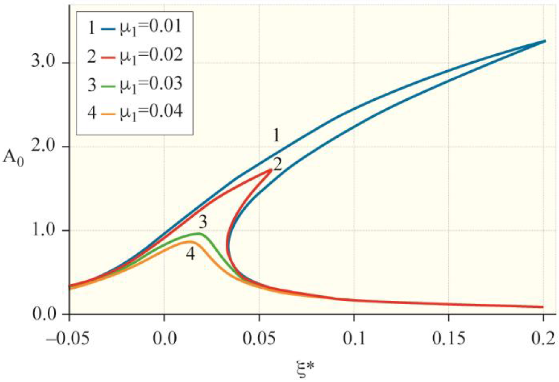
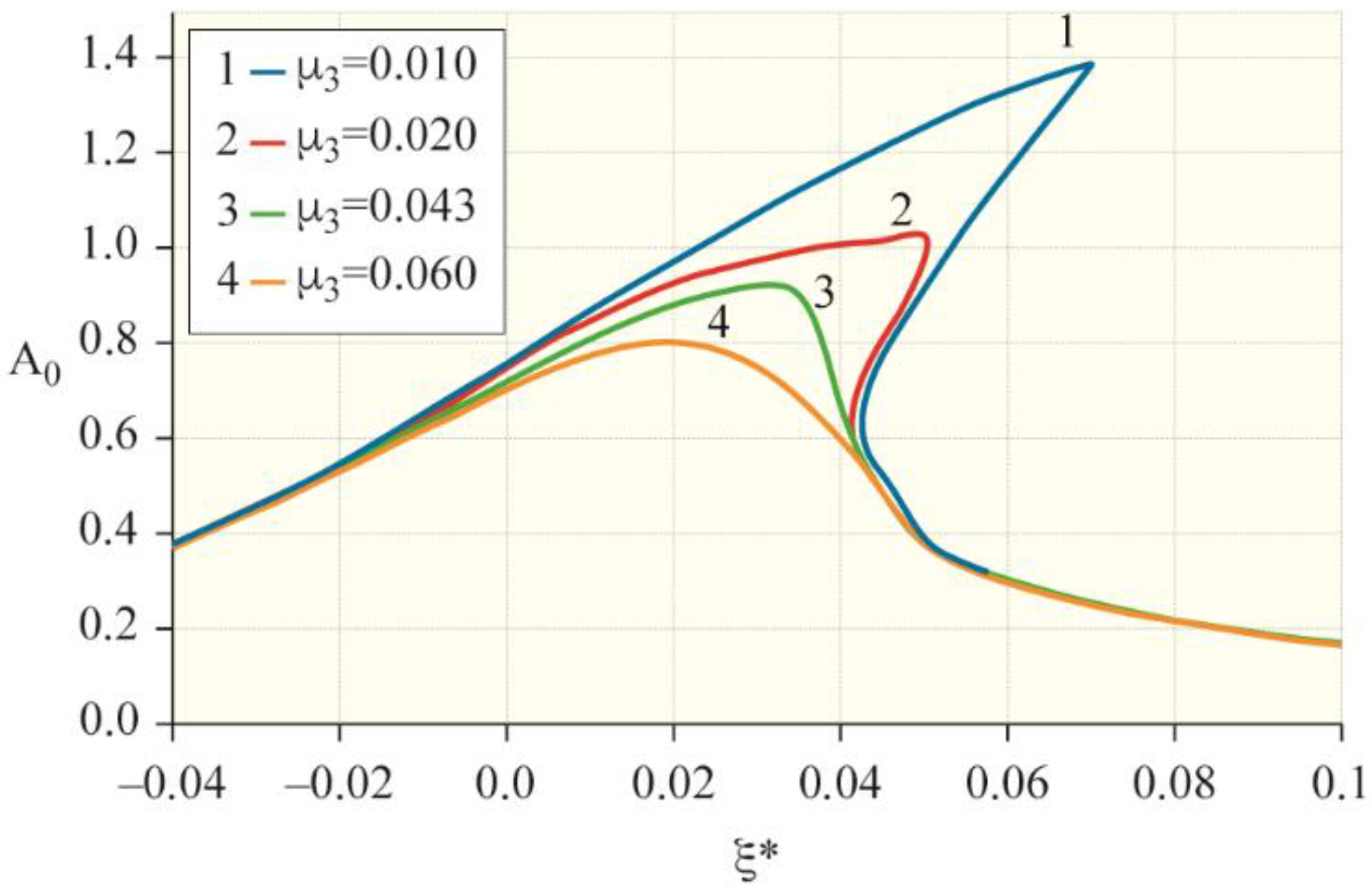
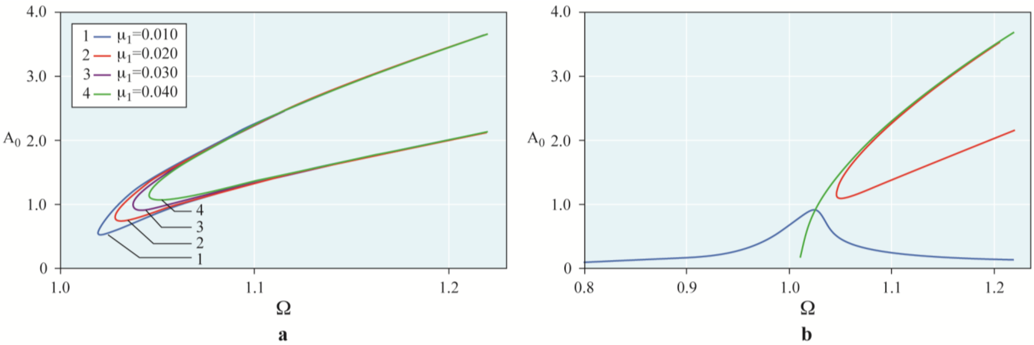
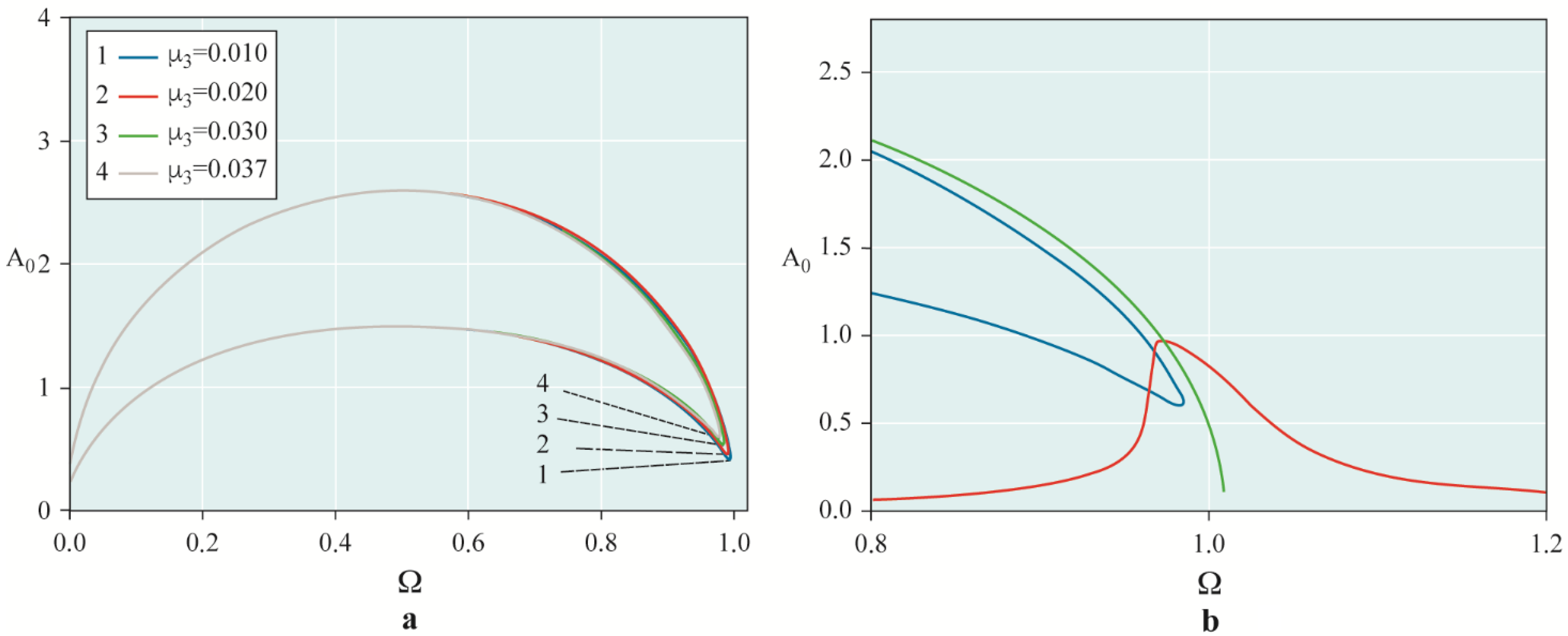
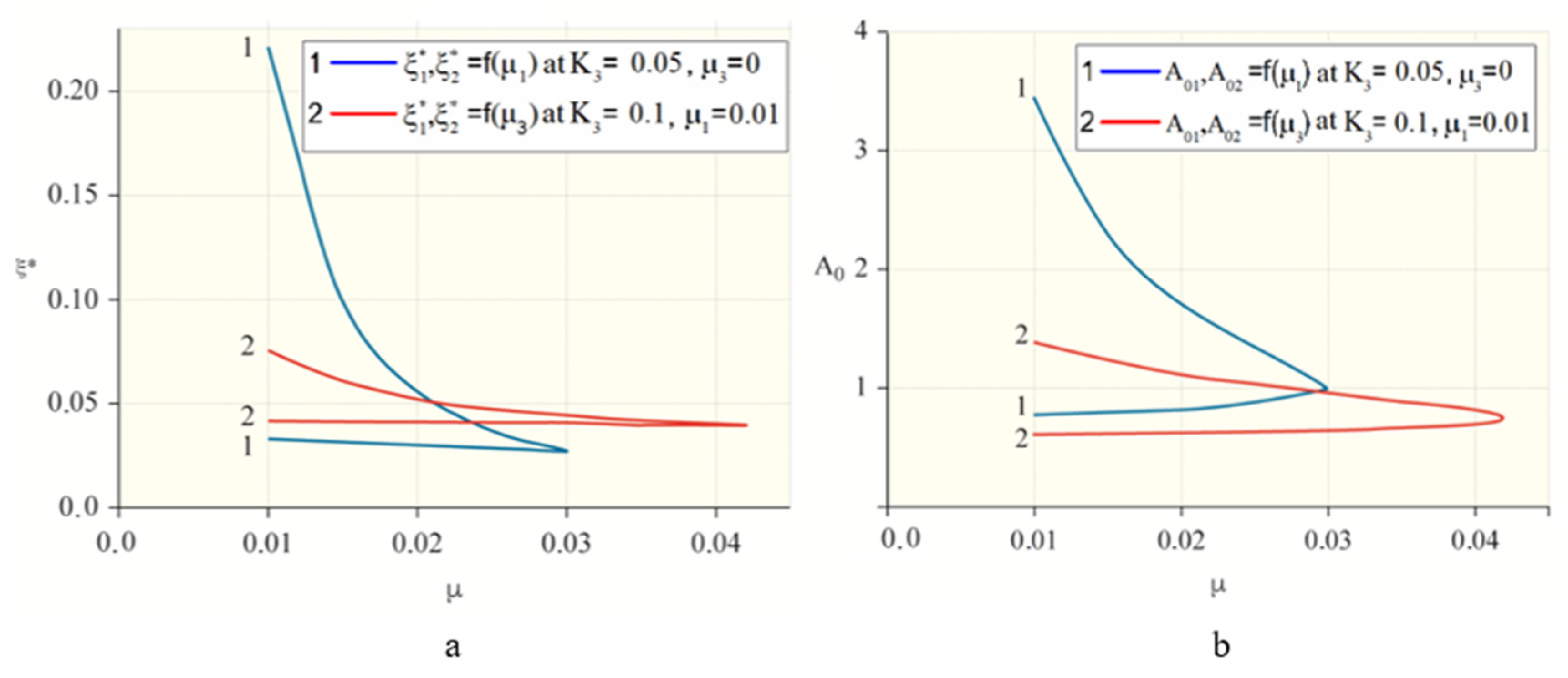
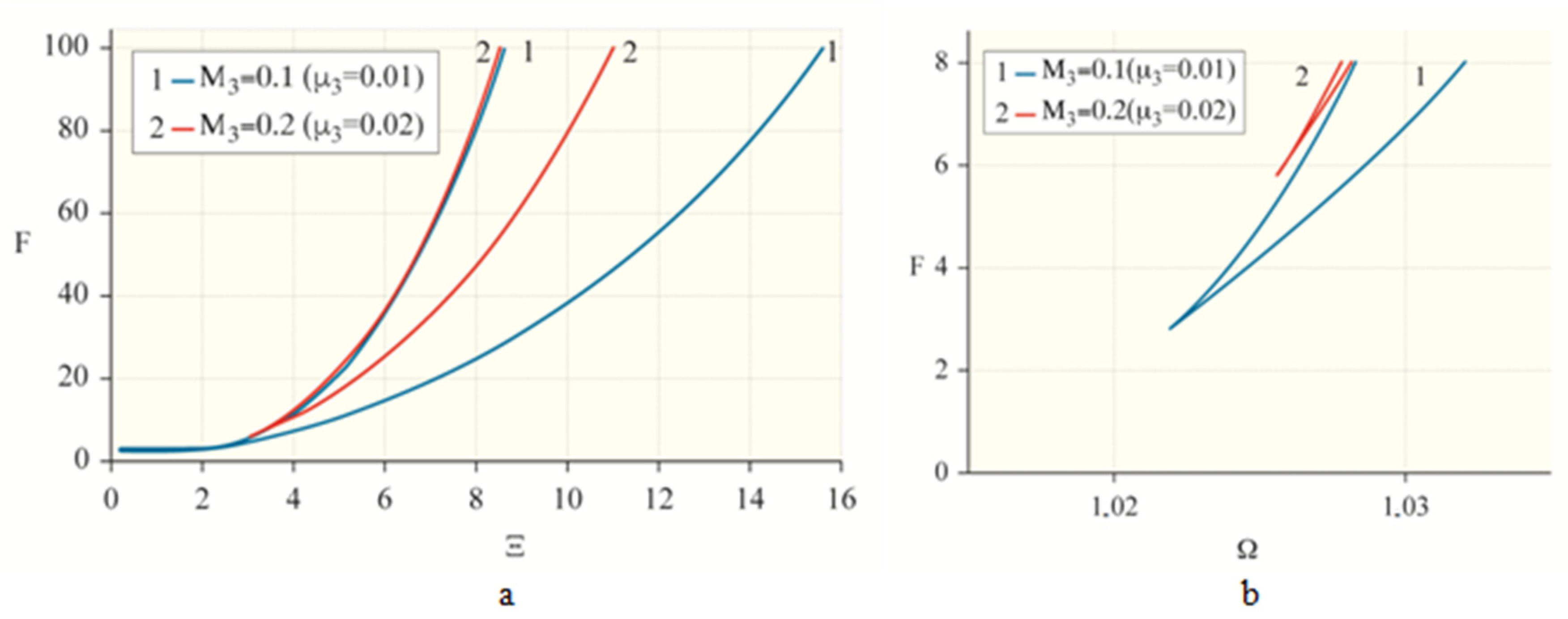
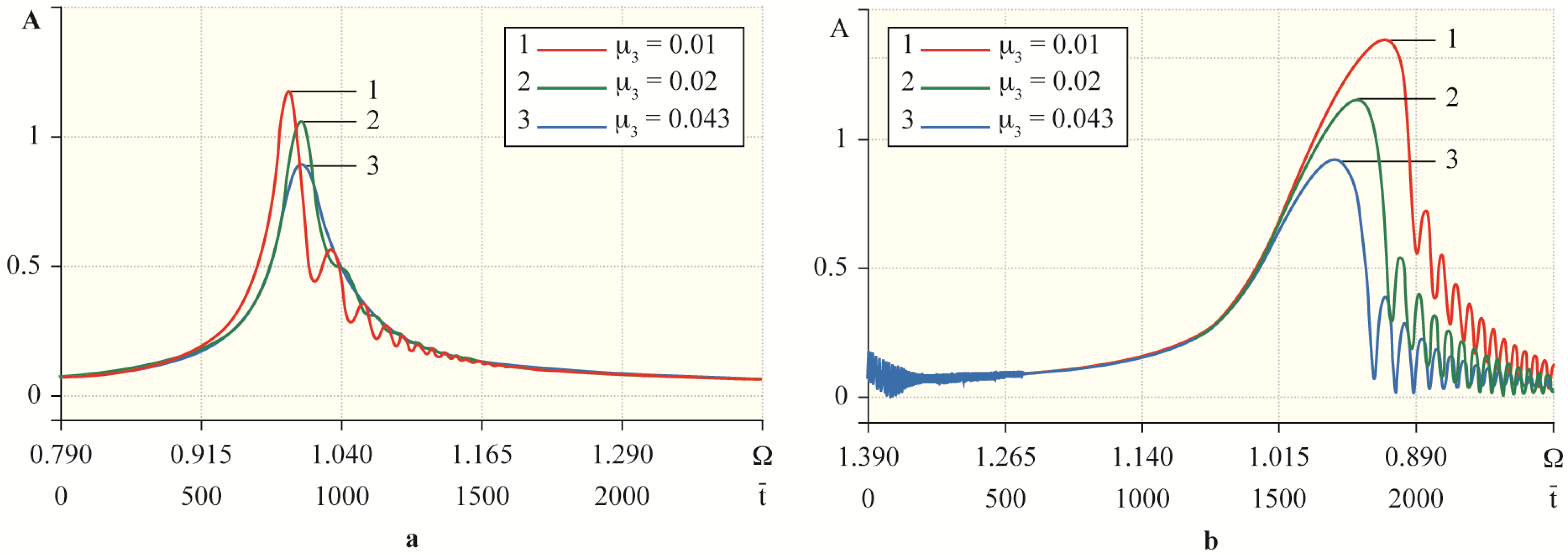
  • It was shown that the combined linear and nonlinear cubic damping significantly reduces the oscillation amplitudes, including the maximum resonant amplitude, and has a greater effect on the boundaries of the bistability region—on the amplitudes and frequencies (shaft rotation speeds) corresponding to jumps—than the linear damping of the support material.
  • A methodology has been developed for determining and identifying the coefficients of linear damping and nonlinear cubic damping of the support material, at which nonlinear jumping effects disappear, for a harmonically forced weakly nonlinear gyroscopic rigid rotor system with a disk with a predominant transverse moment of inertia.
  • It is shown that if linear damping shifts the left boundary of the instability region towards large amplitudes and speeds of shaft rotation, then nonlinear cubic damping can completely eliminate it. In this case, the stability criterion has been obtained by the method of analysis of the characteristic equation in the form of Jacobi and the results of studies of the region of specific points.
  • The resonant transitions and the influence of nonlinear stiffness and nonlinear cubic damping of the support material on the frequency characteristics of a non-stationary process are considered because the VAM was employed to study the response of the rotor system, supplemented by the concept of “slow” time and the parameter “slowly” by changing the angular velocity of rotation.
  • The analytical solutions and numerical solutions of the equations of motion of the rotor show agreement.
  • The results of analytical solutions of the equations of motion are in satisfactory agreement with the results of numerical solutions.
  • The subject of research for the near future is the experimental measurement of parameters of elastic and damping characteristics of samples of material for support and determination of values μ d 1 * and μ d 3 * and theidentification of these parameters, comparison of the results obtained with the results of other models.

Author Contributions

Conceptualization, Z.I.; methodology, Z.I.; software, K.B., N.J. and A.A.; validation, Z.I. and N.J.; formal analysis, Z.I. and K.B.; investigation, Z.I. and K.B.; resources, Z.I. and A.A.; data curation, Z.I., K.B., N.J. and A.A.; writing—original draft preparation, Z.I.; writing—review and editing, Z.I.; visualization, Z.I., K.B., N.J. and A.A.; supervision, Z.I.; project administration, Z.I.; funding acquisition, Z.I. All authors have read and agreed to the published version of the manuscript.

Funding

This research is funded by the Science Committee of the Ministry of Education and Science of the Republic of Kazakhstan (Grant No. AP08856763).

Institutional Review Board Statement

Not applicable.

Informed Consent Statement

Not applicable.

Data Availability Statement

No new data were created or analyzed in this study.

Conflicts of Interest

The authors declare no conflict of interest.

Appendix A

The angular velocity on the coordinate axes can be written in the form
ω N = β ˙ , ω K = α ˙ cos β , ω Z = φ ˙ + α ˙ sin β
Assuming that in the case of small angles α and β sin β β , cos β 1 the previous equations can be rewritten as follows:
ω N β ˙ , ω K α ˙ , ω Z φ ˙ + α ˙ β .
Based on Koenig’s theorem for the kinetic energy of the rotor, we obtain the expression
T = 1 2 m ( x ˙ m 2 + y ˙ m 2 ) + 1 2 ( I K ω K 2 + I N ω N 2 + I Z ω Z 2 ) .
Considering that I K = I N = I T , I Z = I P and considering (A1), we obtain
T = 1 2 m ( x ˙ m 2 + y ˙ m 2 ) + 1 2 I T ( β ˙ 2 + α ˙ 2 ) + 1 2 I P ( φ ˙ + α ˙ β ) 2
where
x m = x + e cos φ = L α + e cos φ , y m = y + e sin φ = L β + e sin φ .
Considering the above, the projections of the angular velocity on the coordinate axes can be written in the form
ω N = β ˙ , ω K = α ˙ cos β , ω Z = φ ˙ + α ˙ sin β
The projections of the moment gravitational and the inertial force of the mass imbalance have the form:
M K = ( L α + e cos φ ) G , M N = ( L β + e sin φ ) G
where G = m g the weight of the disk.
Richards and Singh [3] found that rubber dampers exhibit both nonlinear damping and nonlinear stiffness. To achieve a higher performance, the presence of nonlinearity in the design must be considered. Consequently, the elastic support of the upper bearing of the gyroscopic rotor can be made of non-linear materials such as gum, rubber, and other polymers, which are widely used as vibration dampers. Taking all this into account, we set the dissipative energy in the elastic support in the form of the Rayleigh function
Φ = 1 2 μ d 1 ( α ˙ 2 + β ˙ 2 ) + 1 4 μ d 3 ( α ˙ 4 + β ˙ 4 )
where μ d 1 is the coefficient of linear viscous damping, and μ d 3 is the coefficient of nonlinear cubic viscous damping. Given that the rotor shaft is rigid and only its upper support possesses elasticity, and the elastic forces in mutually perpendicular Ddirections of coordinates are, respectively, equal to F x = k 1 x 0 + k 3 x 0 3 = k 1 l 0 α + k 3 l 0 3 α 3 , , F y = k 1 y 0 + k 3 y 0 3 = k 1 l 0 β + k 3 l 0 3 β 3 , the potential energy of the system can then be represented in the form
V = 1 2 k 1 l 0 2 ( α 2 + β 2 ) + 1 4 k 3 l 0 4 ( α 4 + β 4 )
where k 1 is the stiffness coefficient of the support, and k 3 is the coefficient of the nonlinear term of the elastic force.
Lagrange equations of the second kind for a rotor system can be represented as:
d d t ( T q ˙ i ) T q i + V q i = Φ q ˙ i + Q i .
Here, q i are generalized coordinates; Q i  are generalized forces; i = 1, 2. The generalized coordinates q i , q 2 are α , β . The generalized forces Q i , Q 2 are represented by M K , M N and are determined by (A4).

Appendix B

New variables d α d t ¯ and d β d t ¯ are introduced with respect to the angular coordinates α and β:
d α d t ¯ = A Ω sin ( Ω t ¯ + θ )   and   d β d t ¯ = A Ω cos ( Ω t ¯ + θ ) .
These variables are not the result of differentiating α and β with respect to time t ¯ because the true derivatives of α and β with respect to t ¯ have the form:
d α d t ¯ = d A d t ¯ cos ( Ω t ¯ + θ ) A ( Ω + d θ d t ¯ ) sin ( Ω t ¯ + θ ) ,
d β d t ¯ = d A d t ¯ cos ( Ω t ¯ + θ ) A ( Ω + d θ d t ¯ ) sin ( Ω t ¯ + θ ) ,
Therefore, to be consistent with expressions (18), we have to assume:
d A d t ¯ cos ( Ω t ¯ + θ ) A d θ d t ¯ sin ( Ω t ¯ + θ ) = 0 ,
d A d t ¯ sin ( Ω t ¯ + θ ) + A d θ d t ¯ cos ( Ω t ¯ + θ ) = 0  
These ratios can be considered as additional conditions imposed on variables A   and θ .

Nomenclature

A vibration amplitude, rad
A 0 vibration amplitude in stationary motion mode, rad
e linear eccentricity, m
e r linear eccentricity, dimensionless
G disc weight, N
G ¯ disc weight, dimensionless
I P polar moment of inertia, kgm2
I ¯ P polar moment of inertia, dimensionless
I P 1 polar moment of inertia, comparative, dimensionless
I T transverse moment of inertia, kgm2
I ¯ T transverse moment of inertia, dimensionless
k 1 coefficient of linear stiffness, N/m
K ¯ 1 coefficient of linear stiffness, dimensionless
K 1 linear stiffness coefficient, comparative, dimensionless
k 3 coefficient of nonlinear stiffness, N/m3
K 3 coefficient of nonlinear stiffness, dimensionless
l 0 distance between supports, m
ldistance between supports, dimensionless
L shaft length, m
m disc mass, kg
t ¯ time, dimensionless
α ,   β angular coordinates, rad
θ   vibration phase, rad
μ d 1 coefficient of linear viscous damping, Nms/rad
μ 1 coefficient of linear viscous damping, dimensionless
μ d 3 coefficient of nonlinear cubic viscous damping, N ms3/rad3
μ 3 coefficient of nonlinear cubic viscous damping, dimensionless
ν angular acceleration, dimensionless
ξ frequency detuning, rad
ξ * frequency detuning taking into account the gyroscopic moment, rad
τ ¯ slow time, dimensionless
ω shaft speed, rad/s
Ω shaft speed, dimensionless
ω 0 the natural frequency of the rotary system, rad/s
ω n the natural frequency of the rotary system, dimensionless

References

  1. Zakaria, A.A.; Rustighi, E.; Ferguson, N.S. A numerical investigation into the effect of the supports on the vibration of rotating shafts. In Dynamics of Rotating Systems, Proceedings of the 11th International Conference on Engineering Vibration, Ljubljana, Slovenia, 7–10 September 2015; Boltear, M., Slavi£, J., Wiercigroch, M., Eds.; Faculty for Mechanical Engineering: Ljubljana, Slovenia, 2015; Volume 57, pp. 539–552. [Google Scholar]
  2. Gil-Negrete, N.; Vinolas, J.; Kari, L. A Nonlinear Rubber Material Model Combining Fractional Order Viscoelasticity and Amplitude Dependent Effects. J. Appl. Mech. 2009, 76, 011009. [Google Scholar] [CrossRef]
  3. Richards, C.M.; Singh, R. Experimental characterization of nonlinear rubber isolators in a multi-degree-of-freedom system configuration. J. Acoust. Soc. Am. 1999, 106, 2178. [Google Scholar] [CrossRef]
  4. Matsubara, M.; Teramoto, S.; Nagatani, A.; Kawamura, S.; Tsujiuchi, N.; Ito, A.; Kobayashi, M.; Furuta, S. Effect of Fiber Orientation on Nonlinear Damping and Internal Microdeformation in Short-Fiber-Reinforced Natural Rubber. Exp. Tech. 2021, 45, 37–47. [Google Scholar] [CrossRef]
  5. Ravindra, B.; Mallik, A. Performance of Non-linear Vibration Isolators Under Harmonic Excitation. J. Sound Vib. 1994, 170, 325–337. [Google Scholar] [CrossRef]
  6. Peng, Z.; Meng, G.; Lang, Z.; Zhang, W.; Chu, F. Study of the effects of cubic nonlinear damping on vibration isolations using Harmonic Balance Method. Int. J. Non-Linear Mech. 2012, 47, 1073–1080. [Google Scholar] [CrossRef]
  7. Lang, Z.; Jing, X.; Billings, S.; Tomlinson, G.; Peng, Z. Theoretical study of the effects of nonlinear viscous damping on vibration isolation of sdof systems. J. Sound Vib. 2009, 323, 352–365. [Google Scholar] [CrossRef]
  8. Xiao, Z.; Jing, X.; Cheng, L. The transmissibility of vibration isolators with cubic nonlinear damping under both force and base excitations. J. Sound Vib. 2013, 332, 1335–1354. [Google Scholar] [CrossRef]
  9. Iskakov, Z. Resonant Oscillations of a Vertical Hard Gyroscopic Rotor with Linear and Non-linear Damping. In Advances in Mechanism and Machine Science; Mechanisms and Machine Science; Springer International Publishing: Cham, Switzerland, 2019; Volume 73, pp. 3353–3362. [Google Scholar] [CrossRef]
  10. Iskakov, Z.; Bissembayev, K. The nonlinear vibrations of a vertical hard gyroscopic rotor with nonlinear characteristics. Mech. Sci. 2019, 10, 529–544. [Google Scholar] [CrossRef]
  11. Al-Solihat, M.K.; Behdinan, K. Force transmissibility and frequency response of a flexible shaft–disk rotor supported by a nonlinear suspension system. Int. J. Non-Linear Mech. 2020, 124, 103501. [Google Scholar] [CrossRef]
  12. Fujiwara, H.; Nakaura, H.; Watanabei, K. The vibration behavior of flexibly fixed rotating machines. In Rotor Dynamics, Proceedings of the 14th IFToMM World Congress, 25–30 October 2015; Chang, S.H., Ceccarelli, M., Sung, C.K., Chang, J.Y., Liu, T., Eds.; Airily Library: Taipei, Taiwan, 2015; pp. 517–522. [Google Scholar] [CrossRef]
  13. Li, D.; Shaw, S.W. The effects of nonlinear damping on degenerate parametric amplification. Nonlinear Dyn. 2020, 102, 2433–2452. [Google Scholar] [CrossRef]
  14. Mofidian, S.M.M.; Bardaweel, H. Displacement transmissibility evaluation of vibration isolation system employing nonlinear-damping and nonlinear-stiffness elements. J. Vib. Control 2018, 24, 4247–4259. [Google Scholar] [CrossRef]
  15. Iskakov, Z. Resonant Oscillations of a Vertical Unbalanced Gyroscopic Rotor with Non-linear Characteristics. In Rotor Dynamics, Proceedings of the 14th IFToMM World Congress, Taipei, Taiwan, 25–30 October 2015; Chang, S.H., Ceccarelli, M., Eds.; Airily Library: Taipei, Taiwan, 2015; pp. 505–513. [Google Scholar] [CrossRef]
  16. Iskakov, Z. Dynamics of a Vertical Unbalanced Gyroscopic Rotor with Non-linear Characteristics. In New advances in Mechanisms, Mechanical Transmissions and Robotics; Mechanisms and Machine Science; Springer International Publishing: Cham, Switzerland, 2017; Volume 46, pp. 107–114. [Google Scholar] [CrossRef]
  17. Donmez, A.; Cigeroglu, E.; Ozgen, G.O. The effect of stiffness and loading deviations in a nonlinear isolator having quasi zero stiffness and geometrically nonlinear damping. In Proceedings of the ASME International Mechanical Engineering Congress and Exposition, Tampa, FL, USA, 3–9 November 2017. [Google Scholar]
  18. Balaji, P.S.; Selvakumar, K.K. Applications of Nonlinearity in Passive Vibration Control: A Review. J. Vib. Eng. Technol. 2021, 9, 183–213. [Google Scholar] [CrossRef]
  19. Liao, X.; Sun, X.J.; Wang, Y. Modeling and dynamic analysis of hydraulic damping rubber mount for cab under larger amplitude excitation. J. Vibroeng. 2021, 23, 542–558. [Google Scholar]
  20. Menga, N.; Bottiglione, F.; Carbone, G. Nonlinear viscoelastic isolation for seismic vibration mitigation. Mech. Syst. Signal Process. 2021, 157, 107626. [Google Scholar] [CrossRef]
  21. Dai, Q.; Liu, Y.; Qin, Z.; Chu, F. Nonlinear Damping and Forced Response of Laminated Composite Cylindrical Shells with Inherent Material Damping. Int. J. Appl. Mech. 2021, 13. [Google Scholar] [CrossRef]
  22. Li, H.; Li, J.; Yu, Y.; Li, Y. Modified Adaptive Negative Stiffness Device with Variable Negative Stiffness and Geometrically Nonlinear Damping for Seismic Protection of Structures. Int. J. Struct. Stab. Dyn. 2021, 21, 2150107. [Google Scholar] [CrossRef]
  23. Kong, X.; Li, H.; Wu, C. Dynamics of 1-dof and 2-dof energy sink with geometrically nonlinear damping: Application to vibration suppression. Nonlinear Dyn. 2018, 91, 733–754. [Google Scholar] [CrossRef]
  24. Zhang, Y.; Kong, X.; Yue, C.; Xiong, H. Dynamic analysis of 1-dof and 2-dof nonlinear energy sink with geometrically nonlinear damping and combined stiffness. Nonlinear Dyn. 2021, 105, 167–190. [Google Scholar] [CrossRef]
  25. Taghipour, J.; Dardel, M.; Pashaei, M.H. Vibration mitigation of a nonlinear rotor system with linear and nonlinear vibration absorbers. Mech. Mach. Theory 2018, 128, 586–615. [Google Scholar] [CrossRef]
  26. Mojahed, A.; Moore, K.; Bergman, L.A.; Vakakis, A.F. Strong geometric softening–hardening nonlinearities in an oscillator composed of linear stiffness and damping elements. Int. J. Non-Linear Mech. 2018, 107, 94–111. [Google Scholar] [CrossRef]
  27. Liu, Y.; Mojahed, A.; Bergman, L.A.; Vakakis, A.F. A new way to introduce geometrically nonlinear stiffness and damping with an application to vibration suppression. Nonlinear Dyn. 2019, 96, 1819–1845. [Google Scholar] [CrossRef]
  28. Le Guisquet, S.; Amabili, M. Identification by means of a genetic algorithm of nonlinear damping and stiffness of continuous structures subjected to large-amplitude vibrations. Part I: Single-degree-of-freedom responses. Mech. Syst. Signal Process. 2021, 153, 107470. [Google Scholar] [CrossRef]
  29. Civera, M.; Grivet-Talocia, S.; Surace, C.; Fragonara, L.Z. A generalised power-law formulation for the modelling of damping and stiffness nonlinearities. Mech. Syst. Signal Process. 2021, 153, 107531. [Google Scholar] [CrossRef]
  30. Chatterjee, A.; Chintha, H.P. Identification and parameter estimation of cubic nonlinear damping using harmonic probing and volterra series. Int. J. Non-Linear Mech. 2020, 125, 103518. [Google Scholar] [CrossRef]
  31. Chatterjee, A.; Chintha, H.P. Identification and Parameter Estimation of Asymmetric Nonlinear Damping in a Single-Degree-of-Freedom System Using Volterra Series. J. Vib. Eng. Technol. 2021, 9, 817–843. [Google Scholar] [CrossRef]
  32. Balasubramanian, P.; Ferrari, G.; Amabili, M. Identification of the viscoelastic response and nonlinear damping of a rubber plate in nonlinear vibration regime. Mech. Syst. Signal Process. 2018, 111, 376–398. [Google Scholar] [CrossRef]
  33. Amabili, M.; Balasubramanian, P.; Ferrari, G. Nonlinear vibrations and damping of fractional viscoelastic rectangular plates. Nonlinear Dyn. 2021, 103, 3581–3609. [Google Scholar] [CrossRef]
  34. Amabili, M. Nonlinear damping in large-amplitude vibrations: Modelling and experiments. Nonlinear Dyn. 2018, 93, 5–18. [Google Scholar] [CrossRef]
  35. Lisitano, D.; Bonisoli, E. Direct identification of nonlinear damping: Application to a magnetic damped system. Mech. Syst. Signal Process. 2021, 146, 107038. [Google Scholar] [CrossRef]
  36. Lu, Z.-Q.; Hu, G.-S.; Ding, H.; Chen, L.-Q. Jump-based estimation for nonlinear stiffness and damping parameters. J. Vib. Control. 2019, 25, 325–335. [Google Scholar] [CrossRef]
  37. Al-Hababi, T.; Cao, M.; Saleh, B.; Alkayem, N.F.; Xu, H. A Critical Review of Nonlinear Damping Identification in Structural Dynamics: Methods, Applications, and Challenges. Sensors 2020, 20, 7303. [Google Scholar] [CrossRef]
  38. Parshakov, A.N. Physics of Vibratory Motion; Publishing House of Perm State University: Perm, Russia, 2010; pp. 79–90. [Google Scholar]
  39. Grobov, V.A. Asymptotic Methods for Calculating Bending Vibrations of Turbomachine Shafts; Publishing House of the Academy of Science of the USSR: Moscow, Russia, 1961; pp. 39–79, 95–102. [Google Scholar]
  40. Kuznetsov, A.P.; Kuznetsov, S.P.; Ryskin, N.M. Non-linear vibrations. In Lectures on the Theory of Vibration and Waves; Publishing House of Saratov State University named after Chernyshevsky: Saratov, Russia, 2011; pp. 219–229. [Google Scholar]
  41. Mendeley Date. Available online: https://data.mendeley.com/drafts/ngntc2944b (accessed on 31 October 2021). [CrossRef]
  42. Mendeley Date. Available online: https://data.mendeley.com/drafts/b33zrddfdh (accessed on 31 October 2021). [CrossRef]
  43. Mendeley Date. Available online: http//www.doi.org/10.17632/kcgzh2s5kx (accessed on 31 October 2021). [CrossRef]
  44. Mendeley Date. Available online: https://data.mendeley.com/drafts/f286br875d (accessed on 31 October 2021). [CrossRef]
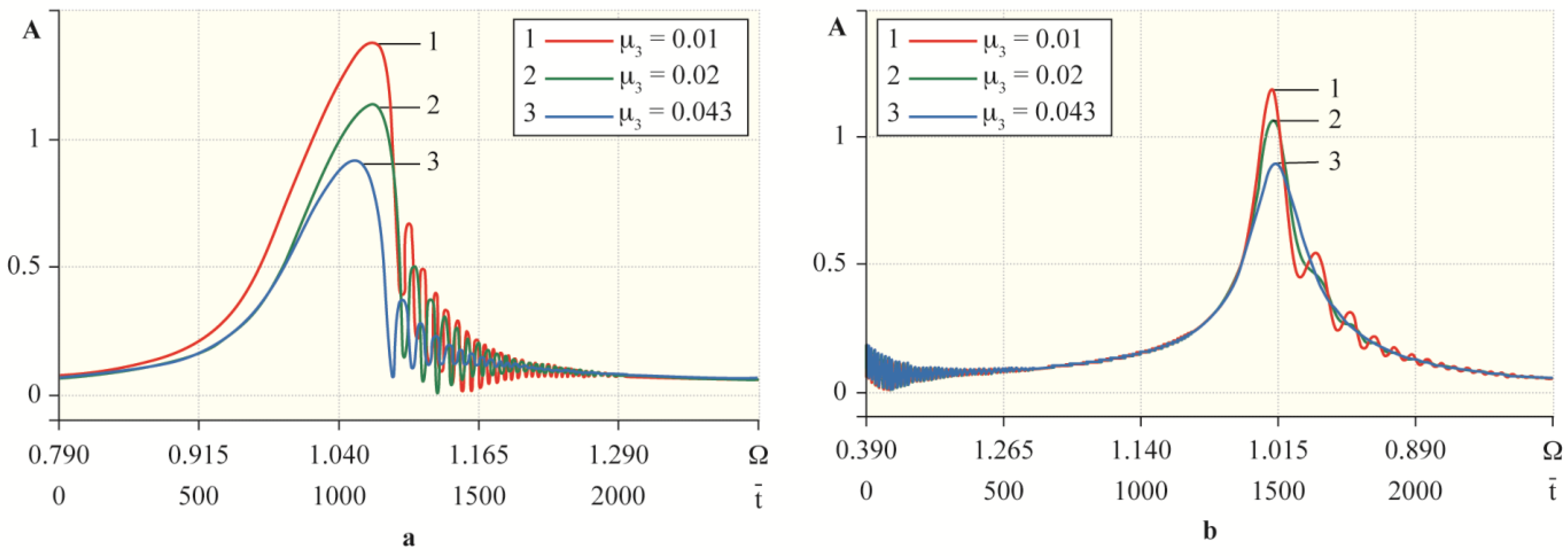
Figure 1. Diagram of the rotor structure.
Machines 09 00276 g001
Figure 2. Dependence A0 = A0(Ω) for a supported rotor with K3 = 0.05 and μ3 = 0 at different values of μ1.
Machines 09 00276 g002
Figure 3. Dependence A0 = A0(Ω) for a rotor with a support with K3 = 0.1 and μ1 = 0.01 at different values of μ3.
Machines 09 00276 g003
Figure 4. Dependence A0 = A0(Ω) with a bistable area at K3 = 0.05, μ3 = 0 and μ1 = 0.01 of support.
Machines 09 00276 g004
Figure 5. Dependence A0 = A0(Ω) with a bistable region at K3 = 0.1, μ1 = 0.01 and μ3 = 0.01 of support.
Machines 09 00276 g005
Figure 6. Responses of the gyroscopic rotor system in solving the equations of motion by different methods: (a)— K 3 = 0.05 and linear damping with μ 1 = 0.04 ; (b)— K 3 = 0.1 and joint damping with μ 3 = 0.043 , μ 1 = 0.01 .
Machines 09 00276 g006
Figure 7. Areas of singular points with boundary lines of a stable (unstable) focus and a stable (unstable) node at 1— μ 1 = 0.01 ,     μ 3 = 0 and 2— μ 1 = 0.01 ,     μ 3 = 0.01 .
Machines 09 00276 g007
Figure 8. Instability regions: (a)—instability regions at μ 3 = 0 , K 3 = 0.05 and different values of μ 1 ; (b)—instability region and frequency response with the vertebral curve at μ 3 = 0 , K 3 = 0.05 and μ 1 = 0.04 .
Machines 09 00276 g008
Figure 9. Instability regions: (a)—instability regions at μ 1 = 0.01 , K 3 = 0.1 and different values μ 3 ; (b)—instability region and frequency response with the vertebral curve at μ 1 = 0.01 , K 3 = 0.1 and μ 3 = 0.037 .
Machines 09 00276 g009
Figure 10. Instability regions: (a)—instability regions at μ 3 = 0 , K 3 = 0.05 and different values of μ 1 ; (b)—instability region and frequency response with the vertebral curve at μ 3 = 0 , K 3 = 0.05 and μ 1 = 0.04 .
Machines 09 00276 g010
Figure 11. Instability regions: (a)—instability regions at μ 1 = 0.01 , K 3 = 0.1 and different values μ 3 ; (b)—instability region and frequency response with the vertebral curve at μ 1 = 0.01 , K 3 = 0.1 and μ 3 = 0.037 .
Machines 09 00276 g011
Figure 12. Graph of the angle α = α ( t ¯ ) during the transition from the initial conditions to the attractor of lower amplitude.
Machines 09 00276 g012
Figure 13. Phase trajectory: α = α ( α ) during the transition process from the initial conditions to a smaller-amplitude attractor.
Machines 09 00276 g013
Figure 14. Graph of the angle β = β ( t ¯ ) during the transition from the initial conditions to the attractor of lower amplitude.
Machines 09 00276 g014
Figure 15. Phase trajectory:   β =   β ( β ) during the transition process from the initial conditions to a smaller-amplitude attractor.
Machines 09 00276 g015
Figure 16. Trajectory of the rotor α = α ( β ) during the transition from the initial conditions to the attractor of lower amplitude.
Machines 09 00276 g016
Figure 17. Trajectory of the rotor α = α ( β ) corresponding to a single oscillation cycle and a time interval: (a)— t ¯ = 306.5 ÷ 327.2 ,   (b)— t ¯ = 425.1 ÷ 445.5 ,   (c)— t ¯ = 700.5 ÷ 714.5 .
Machines 09 00276 g017
Figure 18. The boundaries of the bistability region of the rotor with a support with a rigid characteristic of nonlinear elasticity in the dependencies: (a)— ξ 1 * , ξ 2 * = f( μ i ), (b)— A 01 , A 02 = f( μ i ), i = 1 ,   3 .
Machines 09 00276 g018
Figure 19. The boundaries of the bistability region of the rotor with a support with a soft characteristic of nonlinear elasticity in the dependencies: (a)— ξ 1 * , ξ 2 * = f( μ i ), (b)— A 01 ,   A 02 = f( μ i ), i = 1 ,   3 .
Machines 09 00276 g019
Figure 20. Effect of μ3 on the fold lines (a) and the assemblage point (b).
Machines 09 00276 g020
Figure 21. Dependences of A = A ( t ¯ ) non-stationary oscillations at μ 1 = 0.01 and different values μ 3 .
Machines 09 00276 g021
Figure 22. Dependences of θ = θ ( t ¯ ) non-stationary oscillations at μ 1 = 0.01 and different values μ 3 .
Machines 09 00276 g022
Figure 23. Graph of the angle α = α ( t ¯ ) at μ 3 = 0.01 and = 0.01: 1—based on the results of numerical solution of the Equation (8); 2—based on the results of numerical solution of the Equations (43) and (44).
Machines 09 00276 g023
Figure 24. Graphs of the angle α = α ( t ¯ ) at different values: ( a ) μ 3 = 0.01 ,   ( b ) μ 3 = 0.02 ,     ( c ) μ 3 = 0.043 and at μ 1 = 0.01, based on the results of numerical solution of Equations (43) and (44).
Machines 09 00276 g024
Figure 25. Graphs of the angle α = α ( t ¯ ) at different values: ( a ) μ 3 = 0.01 , ( b ) μ 3 = 0.02 ,     ( c ) μ 3 = 0.043   and at μ 1 = 0.01, based on the results of the numerical solution of Equation (8).
Machines 09 00276 g025
Figure 26. Frequency response of the transient with (a)—ν = 0.00025, (b)—ν = 0.0005 at K 3 > 0 .
Machines 09 00276 g026
Figure 27. Frequency response of the transition process with (a)—ν = 0.00025, (b)—ν = 0.0005 at K 3 > 0 based on the simulation results of Equations (52) and (53).
Machines 09 00276 g027
Figure 28. Frequency response of the transient with c (a)—ν = −0.00025, (b)—ν = −0.0005 at K 3 > 0 .
Machines 09 00276 g028
Figure 29. Frequency response of the transient with (a)—ν = 0.00025, (b)—ν = 0.0005 at K 3 < 0 .
Machines 09 00276 g029
Figure 30. Frequency response of the transient with (a)—ν = −0.00025, (b)—ν = −0.0005 at K 3 < 0 .
Machines 09 00276 g030
Figure 31. Frequency response of the transient with (a)—ν = 0.00025, (b)—ν = −0.00025 at K 3 > 0 .
Machines 09 00276 g031
Figure 32. Frequency response of the transient with (a)—ν = 0.00025, (b)—ν = −0.00025 at K 3 < 0 .
Machines 09 00276 g032
Figure 33. Graph of the angle α = α ( t ¯ ) at the transition process with ν = 0.00025 based on the results of the numerical solution of Equation (49) with: (a)— K 3 > 0 , (b)— K 3 < 0 .
Machines 09 00276 g033
Figure 34. 3D models of: (a)—an elastic support, (b)—a centrifuge based on a vertical rigid gyroscopic rotor.
Machines 09 00276 g034
Figure 35. Structural schemes of a centrifuge based on a rigid gyroscopic rotor (a) and an elastic support (b).
Machines 09 00276 g035
Table 1. Compliance between the oscillatory characteristics: numerical (graphical) values of the peak amplitude A and resonant speed Ω according to the equation of the supporting curve (64).
ω n 1 ,   I P 1 = 0.021 ,   μ 1 = 0.01 ,   ν = 0.00025
K3μ3AΩK3μ3AΩ
0.10.0101.3601.075−0.10.0101.1630.960
0.0201.1251.0600.0201.0500.967
0.0430.9101.0410.0430.9000.980
Publisher’s Note: MDPI stays neutral with regard to jurisdictional claims in published maps and institutional affiliations.

