Article

The Temporal-Spatial Features of Pressure Pulsation in the Diffusers of a Large-Scale Vaned-Voluted Centrifugal Pump

1
College of Water Resources and Civil Engineering, China Agricultural University, Beijing 100083, China
2
Beijing Engineering Research Center of Safety and Energy Saving Technology for Water Supply Network System, China Agricultural University, Beijing 100083, China
3
Dongfang Electric Machinery Co., Ltd., Deyang 618000, China
*
Author to whom correspondence should be addressed.
Machines 2021, 9(11), 266; https://doi.org/10.3390/machines9110266
Submission received: 17 September 2021 / Revised: 19 October 2021 / Accepted: 28 October 2021 / Published: 2 November 2021
(This article belongs to the Section Turbomachinery)

Abstract

:
A large-scale, vaned-voluted centrifugal pump can be applied as the key component in water-transfer projects. Pressure pulsation will be an important factor in affecting the operation stability. This paper researches the propagation and spatial distribution law of blade passing frequency (BPF) and its harmonics on the design condition by numerical simulation. Experimental and numerical monitoring is conducted for pressure pulsation on four discrete points in the vaneless region, which shows that the BPF is dominant. The pulsation tracking network (PTN) is applied to research propagation law and spatial distribution law. It provides a reference for frequency domain information and visualization vaned diffuser. The amplitude of BPF and its harmonics decays rapidly in the vaneless region. BPF and BPF’s harmonics influence each other. BPF has local enhancement in the vaneless region when its harmonics attenuate. In the vaned diffuser, the pulsation amplitude of BPF attenuates rapidly, but the local high-pressure pulsation amplitude can be found on the vane blade concave side because of obstruction and accumulation of the vaned diffuser. In the volute, the pulsation amplitude of BPF is low with the decelerating attenuation. This study provides an effective method for understanding the pressure pulsation law in turbomachinery and other engineering flow cases.

1. Introduction

Large scale centrifugal pumps suit both large flow rate and high head requirements. When applying a large-scale centrifugal pump in liquid delivering, the operation stability is very important due to the contained strong flow energy and its pulsations. In centrifugal pumps, flow is usually fully developed and turbulent, and the flow pulsation performs directly as the pressure and velocity pulsation. It will cause the alternately changing force on the pump body and induce noise, vibration, and damage [1,2,3].
In actual pump and pumping station cases, the pressure pulsation is easy to measure by using pressure pulsation sensors. Especially in stators, sensors can be stably installed by touching the local pulsing flow field. Thus, many researchers tried to study the pressure pulsations at typical positions. By measuring the pressure pulsation in the suction chamber, it was found that this pressure is mainly composed of rotation frequency and other low frequencies [4,5]. Some researchers monitored the volute and studied the influence of cut-water and volute area on pressure pulsations under different working conditions [6,7,8]. The vaned diffuser and vaneless region of pump turbine were respectively measured and studied [9,10,11]. Researchers [12,13] could also measure the pressure pulsation caused by rotating stall phenomenon by arranging sensors at the impeller outlet. Low frequency bands could be well acquired and recognized. Among them, the blade-excited frequencies are always found dominant because the impeller pumps liquid periodically. Liquid obtains energy from impeller blades and flows downstream. The turbulent flow pulses, propagates, and attenuates not only streamwise but also in the secondary directions, which makes a more complex flow. Unfortunately, researchers cannot measure the pressure pulsation everywhere in the flow field. Several discrete monitors can only show the local amplitude of the blade-excited frequencies. The propagation and attenuation details, especially the spatial distribution of temporal states, are still unknown.
Computational fluid dynamics (CFD) is a method that is used widely to analyze the flow pattern and regime with a computer. By using the correct solution method and choosing an appropriate and accurate turbulence model, accurate results matching the experimental results can be obtained. For the single-stage centrifugal pump, most of the research focuses on the rotor-stator interaction and rotation stall. There will be a high amplitude of pressure pulsation with the condition deviating from the design point [1]. Due to the interaction between the vaned diffuser and volute, blade passage frequency and its high-order harmonics were dominant downstream of the impeller [14,15,16,17]. The amplitude of blade passing frequency was affected by the position of cut-water and the distance between the impeller trailing edge and cut-water [15,16]. However, in some flow conditions, due to rotating stall and other reasons, various forms of vortex structures appeared downstream and produced a lower dominant frequency [16,17], which was also affected by volute cut-water [13]. Cavitation can also cause pressure pulsation. Researchers have focused on the relationship between cavitation and pressure pulsation. It was found that cavitation has a strong influence on the amplitude of pressure pulsation under partial-load conditions [18]. When cavitation occurred, the dominant frequency changed from blade passing frequency (BPF) to a lower frequency [19]. In axial-flow pump cases, the maximum pressure pulsation may be upstream to the impeller inlet, and in vaned diffuser channels it will mainly be with the BPF. The pressure pulsation amplitude distributes non-uniformly along a spanwise direction. When the axial-flow pump operated off-design, pressure pulsation amplitude became higher [20,21]. The vortex structure formed by the leading-edge separating flow in a vaned diffuser could cause strong pressure pulsation, which is up to 3~4 times higher than that in the vaneless region [22]. For double-suction centrifugal pumps, pressure pulsation in a semi-spiral suction chamber, impeller, and volute was found dominated by impeller frequency and lower frequency bands, while volute was being dominated by BPF [10]. During the start-up process, pressure pulsation was dominated by impeller frequency, low frequency broadband, and BPF and its harmonics [23]. The impeller blade distributions of a double-suction centrifugal pump also have a significant impact on the amplitude of pressure pulsation. Research shows that an alternative distribution of the blade is helpful to reduce the amplitude of pressure pulsation [24,25]. For pump turbines, the pressure pulsation is mainly affected by a rotor-stator interaction in the vaneless region. The frequency of pressure pulsation is also mainly the BPF. The BPF attenuates rapidly both upstream (to the draft tube) and downstream (to volute) under the influence of a vaned diffuser opening [26,27,28]. In other fields, CFD is also widely used to analyze pressure pulsation. Farzaneh-Gord [29] et al. researched a snubber between the turbine flow meter and the reciprocating compressors by CFD to decrease flow pulsation effects. Lai [30] et al. analyzed the Francis turbine pressure pulsation by CFD.
The method to weaken pressure pulsation is studied widely. Wu [31] et al. weakened the pressure pulsation by modifying the blade pressure side for uniform energy distribution. Lin [32] et al. used a Sinusoidal Tubercle Trailing-Edge to weaken the pressure pulsation caused by rotor-stator interaction. Posa [33] found that the wide rotor-stator clearance weakened the pressure pulsation in the vaneless region. Wang [34] et al. used alternate loading methods to weaken pressure pulsation. Zeng [35] et al. weakened the pressure pulsation by the positive lean mode. Tanasa [36,37,38,39] studied the flow-feedback technique, pulsating jet technique, adjustable diaphragm method, and axial water jet method to weaken the pressure pulsation of the vortex rope.
Generally, in these numerical predictions for the engineering, the internal flow at the pump’s design-load is proven accurate with the unsteady Reynolds-averaged Navier–Stokes (URANS) method [14]. By using the URANS method, the temporal characteristics of pressure pulsation can be well captured at typical points. The BPF is already found dominant and important. However, understanding the spatial distribution of pressure pulsation and other temporal characteristics i4s still difficult. There are great challenges such as the computational cost, arrangement law of monitoring points, setup of pre-processing, resolution of visualization, and algorithms of post-processing.
Considering the disadvantages above, the pulsation tracking network based on the program that is compiled is used. The research object is a large scale vaned-voluted (with both a vaned diffuser and a volute as a diffuser) centrifugal pump that is used in the water transfer project. The accuracy of the calculation is verified by experiment. The blade-excited frequencies are deeply focused towards the downstream region of the impeller, which covers vanes, volute, and cut-water. The pulsation amplitude, phase, dominant frequencies, propagation, and attenuation are analyzed in detail. The generation, propagation, and attenuation of blade-excited frequencies are numerically investigated. It gives a completely new view of the turbulent flow inside the pump and provides new ideas for solving the operation stability problems in pump and pumping station engineering cases.

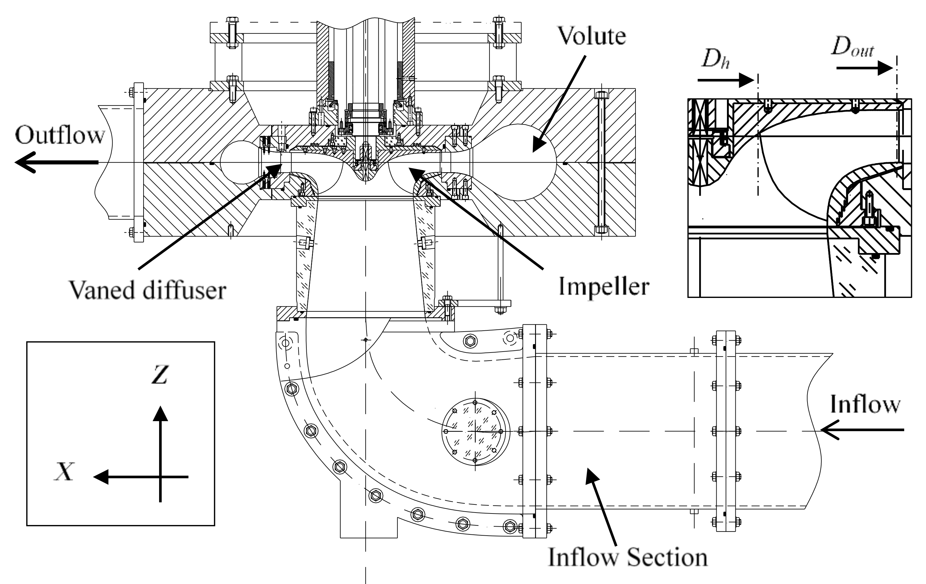
2. Pump Model and Experimental Setup

2.1. Parameters and Condition

In this research study, a large-scale vaned-voluted centrifugal pump unit is studied in model scale. The pump model consists of four parts that are inflow section, impeller, vaned diffuser, and volute. The vaned diffuser is designed for guiding water and supporting the weight of the shaft system and motor. The volute is designed for flow guidance and energy recovery. Figure 1 shows the schematic map of the pump model with the indication of the components. Coordinate X-Y-Z is defined for analysis, where X is the inflow and outflow direction, and Z is the axial direction. The design parameters and geometric parameters are listed in Table 1.
In Table 1, the specific speed n q is an important similarity parameter for comparison among similar pump units. It can be defined as:
n q = n d Q d H d 3 / 4
where Q d is the design flow rate (m3/s), H d is the design head (m), and n d is the design rotational speed (r/min). The dimensionless flow rate coefficient φ , the dimensionless head coefficient ψ , the efficiency of the pump η , the dimensionless coefficient of pressure C p , and the pressure pulsation dimensionless coefficient of A p are defined as:
φ = Q π ω r R o u t   3
ψ = 2 g H π ω r 2 R o u t 2
η = η h η m η v
C p = p p 0.5 ρ ω r 2 R i o u t   2
A p = Δ p 0.5 ρ ω r 2 R o u t   2
where Q is the flow rate (m3/s), H is the head (m), ω r is the rotation angular speed of the impeller (rad/s), R i o u t   is the impeller outlet radius (mm), p is pressure (Pa), p is the reference pressure at the inflow inlet (Pa), Δ p is the difference between instantaneous and average pressure value (Pa), ρ is the fluid density (m3/kg), η h is the hydraulic efficiency, η v is the volume efficiency, and η m is the mechanical efficiency. In this case, the flow rate coefficient and head coefficient are φ d = 0.092 and ψ d = 0.225.

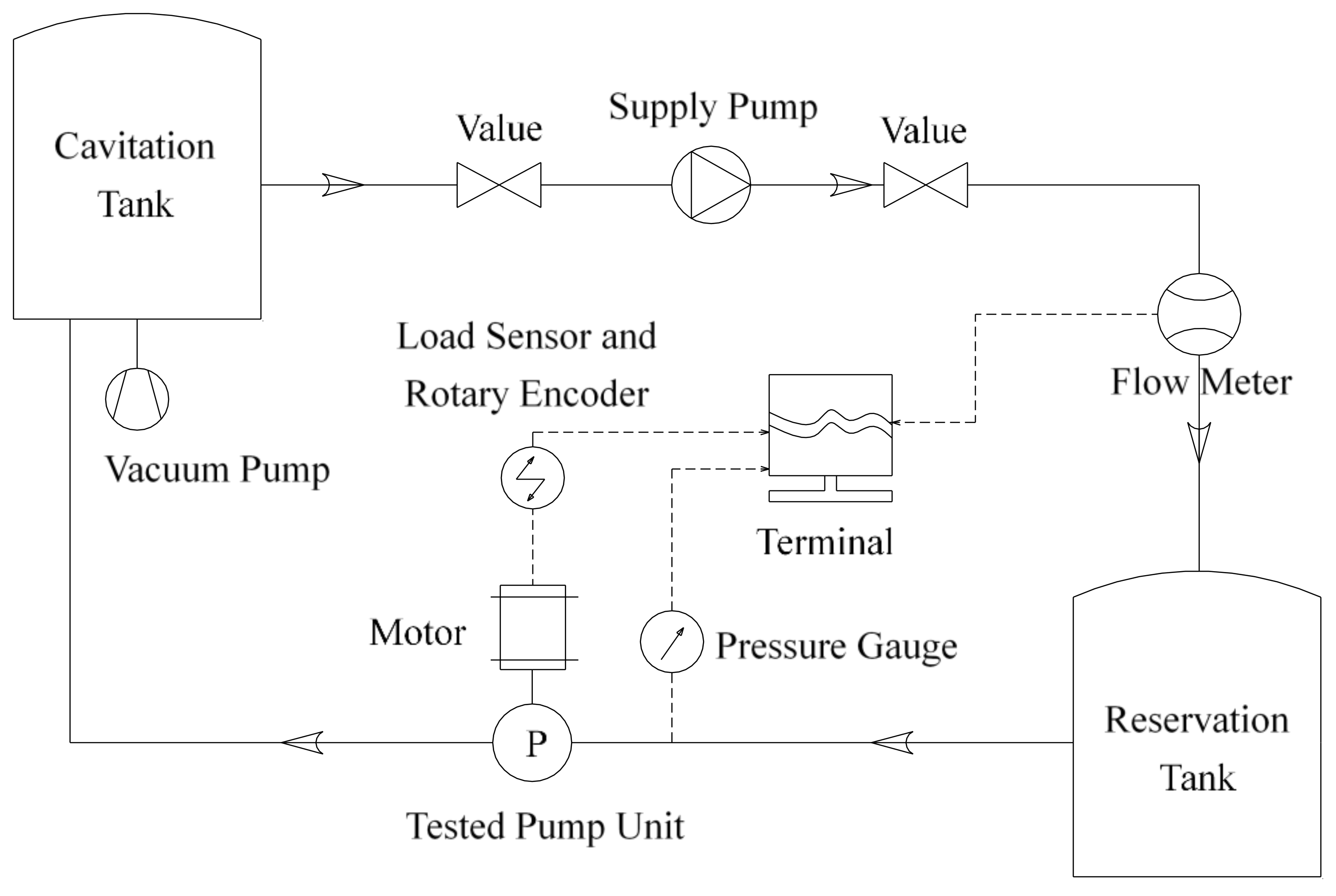
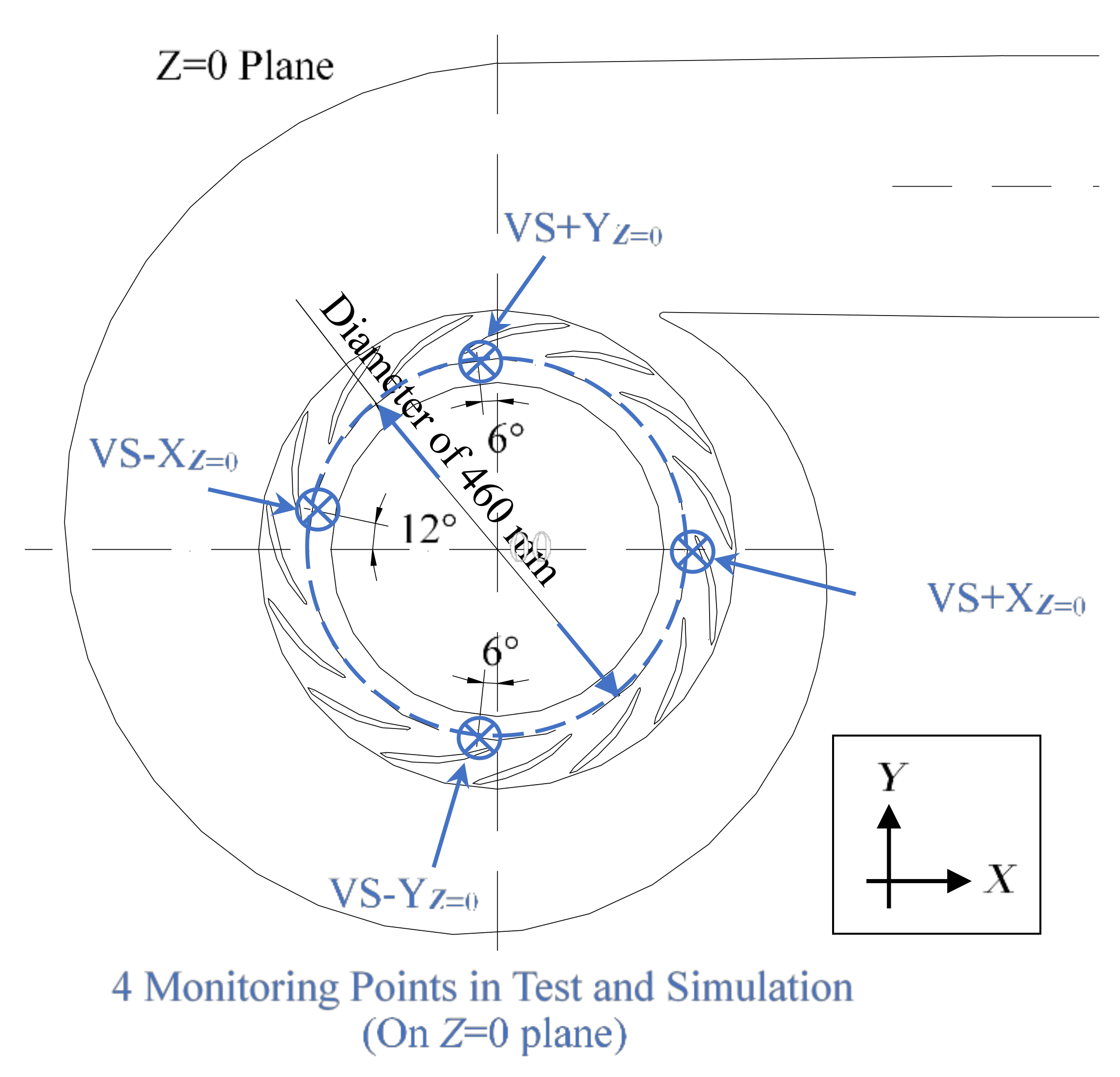
2.2. Model Test Rig, Apparatus, and Method

An experimental study was conducted on the test rig shown in Figure 2. The guideline of the test acceptance procedure is IEC-60193-1999 [40]. Physical quantities including flow rate, head, efficiency, and pressure pulsations were measured. The sampling frequency f s a p of the transient pressure sensor is 2000 Hz, and the total acquisition time t a c q is 12 s. Four pressure pulsation sensors were installed at the top of the vaneless region, as shown in Figure 3. They are denoted as VS + X, VS + Y, VS − X, and VS − Y based on the X-Y-Z coordinate. Due to the inconvenience of installation, the four sensors are deviated from X and Y axes. The deviation angles can be also found in Figure 3. The total uncertainty E can be decomposed into the systematic uncertainty E s and random uncertainty E r as:
E = E r 2 + E s 2
According to the efficiency measurement, it is with an uncertainty of less than ±0.25%. In detail, the apparatus with their types and uncertainties in the test are listed in Table 2.

3. Numerical Simulation Method

3.1. Governing Equations and Turbulence Model

In this calculation, based on the URANS equation and CFD, the three-dimensional incompressible flow is numerically simulated. Because the fluid is incompressible, the continuity equation and momentum equation under the URANS method are as follows:
u ¯ i x i = 0  
ρ u ¯ i t + ρ u ¯ i u ¯ j x j = p x j + μ x j u ¯ i x j + u ¯ j x i ρ u i u j ¯ x j
where u ¯ i is the average velocity, u i is the fluctuating velocity, p is the pressure, t is the time, ρ is the density, μ is the dynamic viscosity, and x i is the spatial coordinate.
According to these two equations, the pressure field and the velocity field can be solved out. However, the Reynolds average equations are not closed. Therefore, the turbulence model should be chosen to make the equation closed. The k-ε model [41] can simulate the complex flow, especially in the free shear layer. However, this model is hard to reflect the turbulence anisotropy characteristics. It is inaccurate to simulate the separated flow. RNG k-ε model [42] and Realizable k-ε model [43] can be better to deal with separated flow and swirling flow. There are strict requirements for the first layer of mesh at the boundary layer for these models. Wilcox k-ω model [44] improves the simulation of a low Reynolds number flow near the boundary layer, which can improve the applicability of the model and predict the flow separation phenomenon with reverse pressure gradient accurately. The Wilcox k-ω model is very sensitive for the ω value of free flow. The BSL k-ω model [45] combines Wilcox k-ω model and k-ε model by blending functions to solve the problem. However, the BSL k-ω model does not consider the transmission effect of turbulent shear stress. The SST k-ω model [45] remedies this defect by eddy viscosity coefficient correction. The SST k-ω model retains the advantages of the k-ω model in the boundary layer and k-ε model in the free shear layer. Many research results show that the SST k-ω model has higher accuracy than other RANS models [46,47,48]. The SST k-ω model is adopted as the turbulence model to close the Reynolds-averaged Navier–Stokes (RANS) equations by establishing the relationship between Reynold’s stress and eddy viscosity. The kinetic energy k equation and specific dissipation rate ω equation are as follows:
( ρ k ) t + ρ u i k x i = P k β * ρ ω k + x i μ + σ k μ t k x i
( ρ ω ) t + ρ u i ω x i = P ω β ρ ω 2 + x i μ + σ ω μ t ω x i + 2 1 F 1 ρ σ ω 2 1 ω k x i ω x i
where P k is the production term of turbulent kinetic energy, P ω is the generating term of the specific dissipation rate. Parameters β , β * , σ k , and σ ω are constants of the turbulence model, μ is the dynamic viscosity, and F1 is the blending function. The turbulent eddy viscosity μ t is defined as follows:
μ t = a 1 k ρ max a 1 ω , S F 2
where a 1 is a constant coefficient, S is an invariant measure of the strain rate, and F 2 is a second auxiliary function within 0~1. In this paper, fast Fourier transform (FFT) [49] is used for time-frequency analysis.

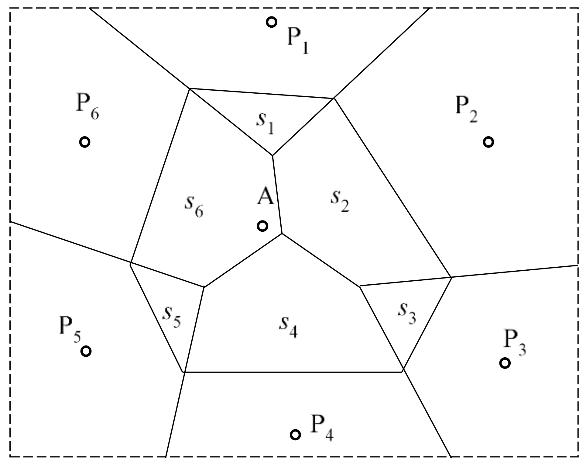
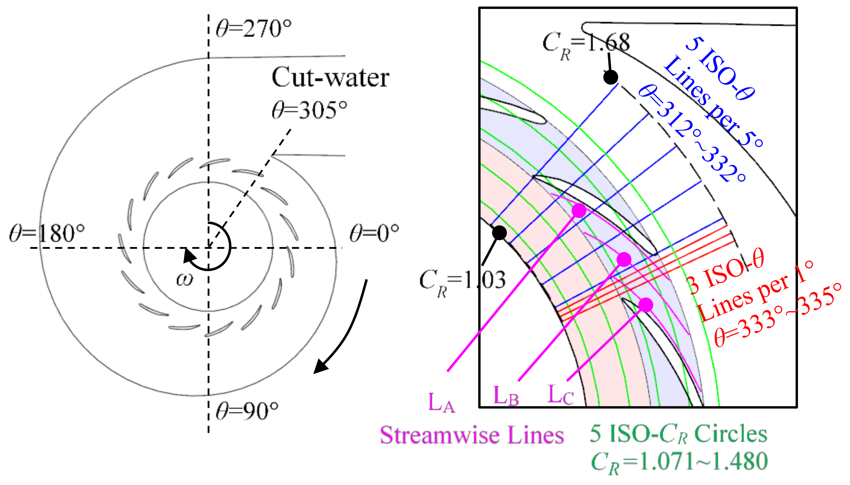
3.2. Pulsation Tracking Network (PTN) with Fourier Transform

Pulsation tracking can be applied to analyzing and visualizing the unknown frequencies. It clarifies the spatial distribution of temporal states in a high resolution. In this case, the pressure pulsation is mainly focused. Hence, the time-frequency conversion is necessary, and the fast Fourier transform is considered as a well-known way in engineering cases. The Fourier series (cosine signal form) of trigonometric function form of X T ( t ) is as follows:
X T ( t ) = C 0 + n = 1 N c n cos ( n ω f t + φ n )
where c n are the amplitude component, ω f is the angular frequency, φ n is the initial phase angle of each sinusoidal function, C 0 is a constant term that represents a deviation from zero, and n is the integer from 1 to infinity. In this way, a complex period signal can be divided into several cosine (or sine) signals with different frequencies. Among them, each frequency component is mainly composed of three important elements that are amplitude c n , frequency ω f , and phase φ n , which determine the shape of the signal. Among them, c n determines the amplitude and the proportion of frequency division in the whole signal, ω f determines its fundamental nature, and φ n determines the state at the initial time or the specific temporal state.
In the traditional time-frequency analysis, the amplitude c n and frequency n ω are mainly concerned. By using this innovative PTN method, all three of the above important elements of time-frequency transformation can be specifically focused on. Well-ordered monitoring points can be arranged with a spatial high resolution. The arrangement is based on both the domain geometry and the CFD mesh node distribution. By arranging large amounts of well-ordered monitoring points, the pressure pulsation in the diffuser from the vaneless region to the volute can be detected. It can be effective to find out the source, propagation law, and attenuation law of pressure pulsation.
Spatial interpolation realizes the ability of continuous surface modeling based on discrete sampling points and estimates the variables in the unsampled area at the same time. It is a powerful method to analyze and deal with the spatial distribution and change trend. As illustrated in Figure 4, the natural neighbor interpolation is an interpolation method based on spatial auto correlation. It is widely used in the research field with the formula as follows [50]:
g ( a ) = i = 1 n w i ( a ) f i
where g ( a ) is the result of interpolation at the point A to be interpolated, w i a is the weight of the interpolation point A about the sample point P i (i = 1, …, n), and f i is the value at the sample point P i . The weight is determined by the following formula:
w i ( a ) = s i s a s a
where s i is the area of the polygon where the sample points participate in the interpolation, and s a is the area of the polygon where point A is to be interpolated. Thus, the variable size of the required point can be obtained, which is convenient to observe the spatial distribution of pressure fluctuation or other temporal states.

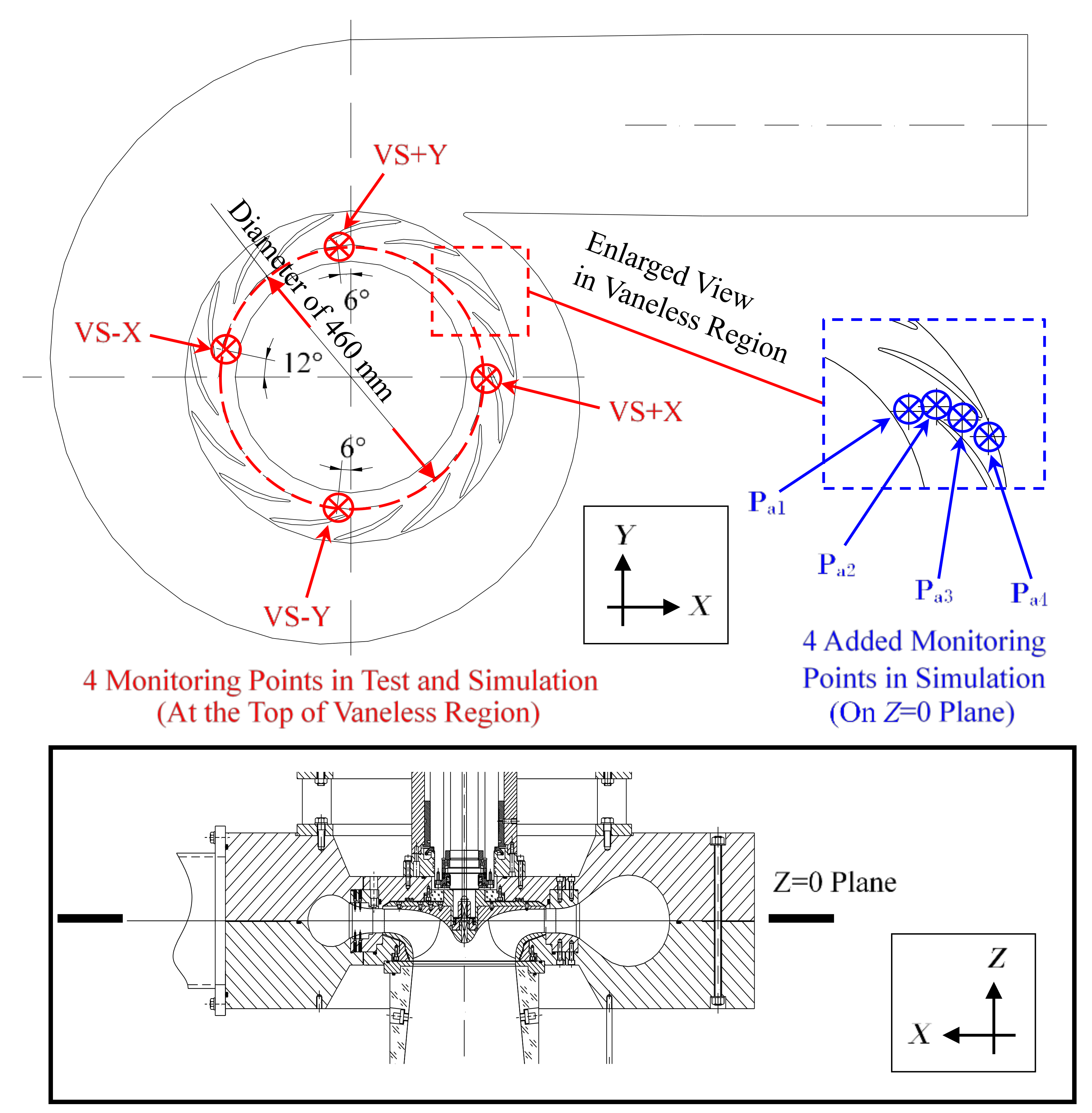
3.3. Setup of PTN in Diffusers

In this study, PTN is set in the vaneless region, vaned diffuser, and volute on the Z = 0 plane, which is also the mid-span of vaned diffuser as shown in Figure 5. The distribution of points is based on the vane and volute geometry and the CFD mesh distribution. Considering the influence of the vane blade, PTN is relatively dense in the vaned diffuser and coarse in the volute. The minimum space between each two PTN points are not smaller than the local CFD meshes space. The maximum space between each two PTN points depends on the local resolution. There are 12,030 monitoring points in the vaneless region and vaned diffuser, and there are 6441 monitoring points in the volute. Therefore, in total, 18,471 monitoring points are arranged as indicated. The monitoring points are distributed based on the mesh node distribution. PTN monitoring can be executed based on transient CFD simulation within a total of 10 impeller revolutions. According to the pressure pulsation data on each point, the spatial distribution and variation can be analyzed by applying interpolations.

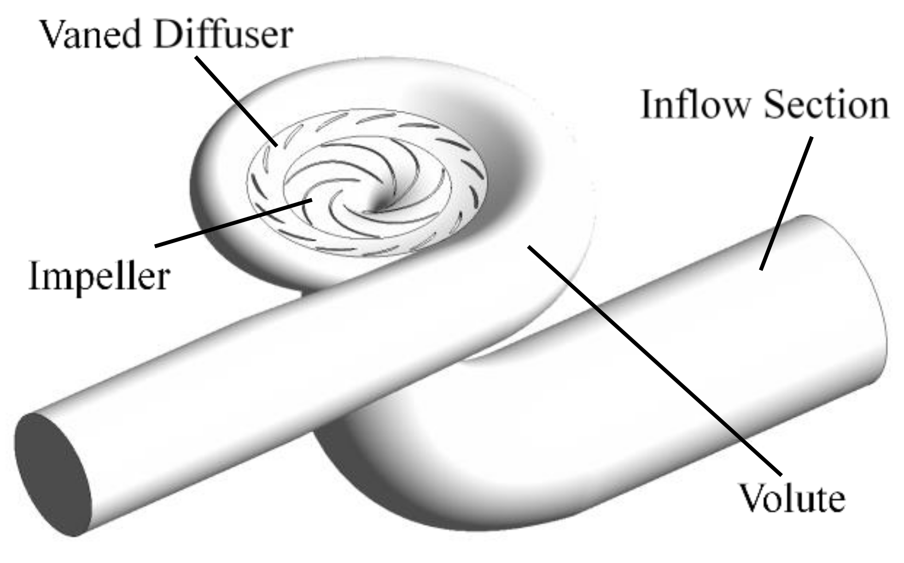
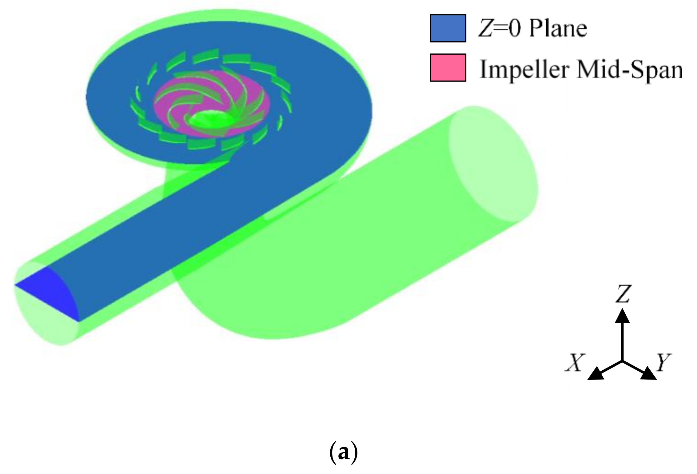
3.4. Flow Domain Modeling

The computational domain of the pump model is shown in Figure 6. It consists of an inflow section, impeller, vaned diffuser, and volute. These domains are discretized by finite volume method with high quality hexahedral elements. The boundary layer meshing of all domains is considered. Complex geometric regions are also locally refined.

3.5. Setup of CFD

The CFD simulation was based on ANSYS CFX. The impeller was defined as a rotating domain by 1200 r/min and others were defined as stationary under the multiple reference frame. Environment pressure was set as 101,325 Pa. The fluid medium was water at 25 °C, which did not involve energy exchange. A mass flow inlet boundary was set at the inlet interface of inflow section, and a static pressure outlet boundary was set at the volute outlet interface. All the walls were set as non-slip wall boundaries. General grid interface (GGI) was used as a grid connection between the two domains. The convergence criterion was the root mean square residual (RMS) of the momentum equation and the continuity equation less than 5 × 10⁻⁵. The steady CFD result was set as the initial condition. Then, the following transient simulation simulated 10 impeller revolutions. The time of the impeller rotating a circle was divided to 720-time steps. And the per time step was divided to 10 iterations. The total time was 0.5 s.

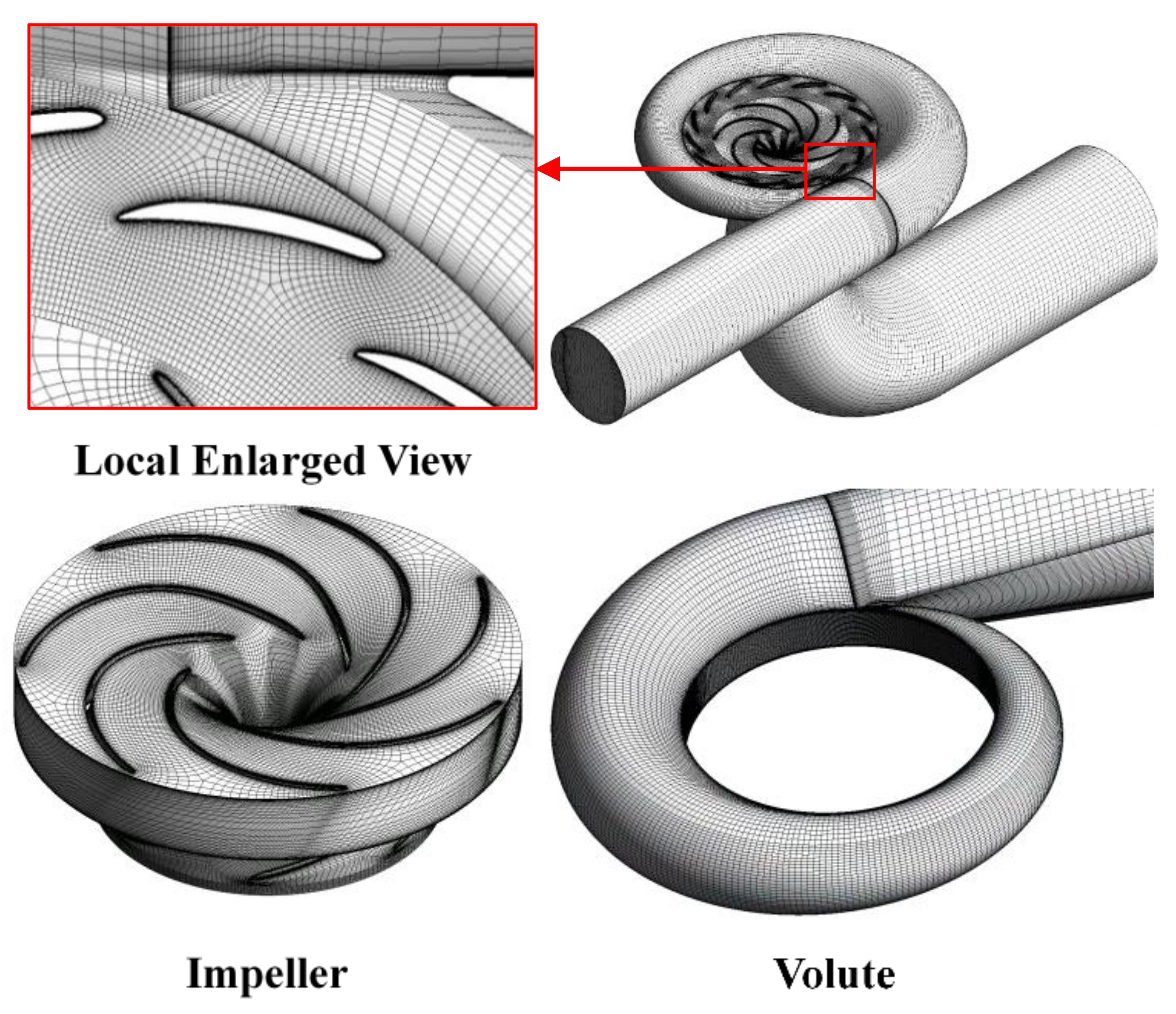
3.6. Flow Domain Meshing and Checking

The grid convergence analysis was conducted using the Grid Convergence Index (GCI) method based on the Richardson extrapolation method [51] for the precision of the simulation. Three mesh schemes of fine mesh (M1), medium mesh (M2), and coarse mesh (M3) were determined in the mesh refinement ratio, which is about 1.3. The elements number of M1, M2, and M3 are 3473556, 1466672, and 554149. Because the research object is the characteristics of pressure pulsation in the vaneless region, the head and the efficiency of the pump and the pressure at the points VS + XZ=0, VS + YZ=0, VS − XZ=0, and VS − YZ=0 (as shown in Figure 7) are taken as the parameters to compare as shown in Table 3. In this table, ϕ 1 ~ ϕ 3 are evaluated variables, p is the observation accuracy order, ϕ ext 21 and ϕ ext 32 are extrapolated values, e ext 21 and e ext 32 are the relative error of the extrapolated values, and GCI fine 21 and GCI fine 32 are the convergence index of the grid. For the different key parameters between M1 and M2, the relative errors of extrapolated values are between 0.06% and 6.2%. The grid convergence index is between 0.07% and 8.3%. Obviously, the M1 and M2 mesh schemes meet the requirement of convergence criteria, and the accuracy of the simulation can be well guaranteed.
The best mesh scheme has the higher prediction accuracy and better capture-ability of the flow details. However, it has a high computational cost, which should be considered. In this case, the fine mesh M1 can be accepted to have an accurate simulation. The detailed information of mesh node and element number is shown in Table 4. The meshing result of M1 is shown in Figure 8. In this study, the values of y+ are about 10–30 for the majority of the areas on the surface of the flow domain. The maximum values of y+ on the surface of inflow, impeller, vaned diffuser, and volute are approximately 100, 150, 300, and 350.

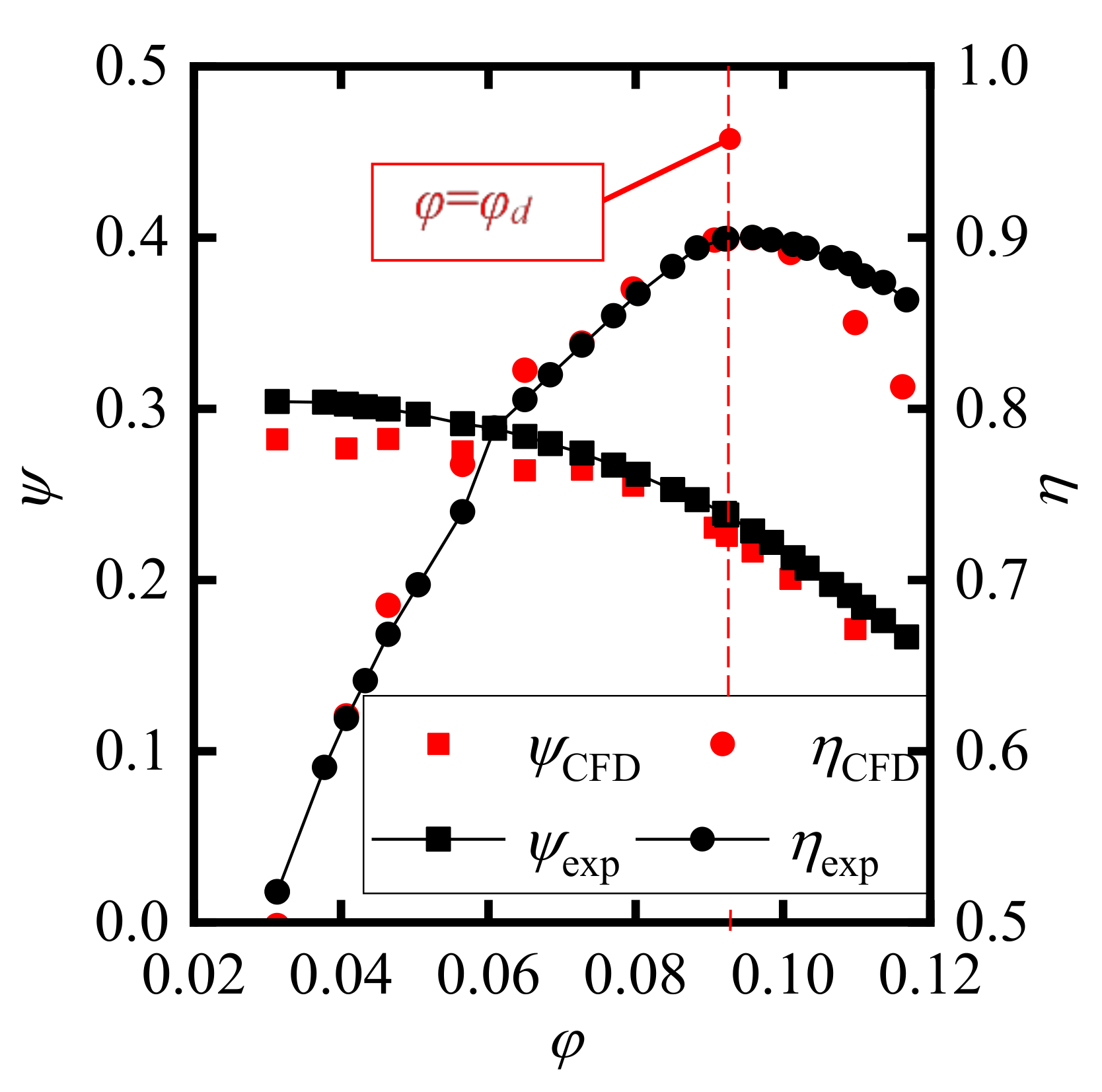
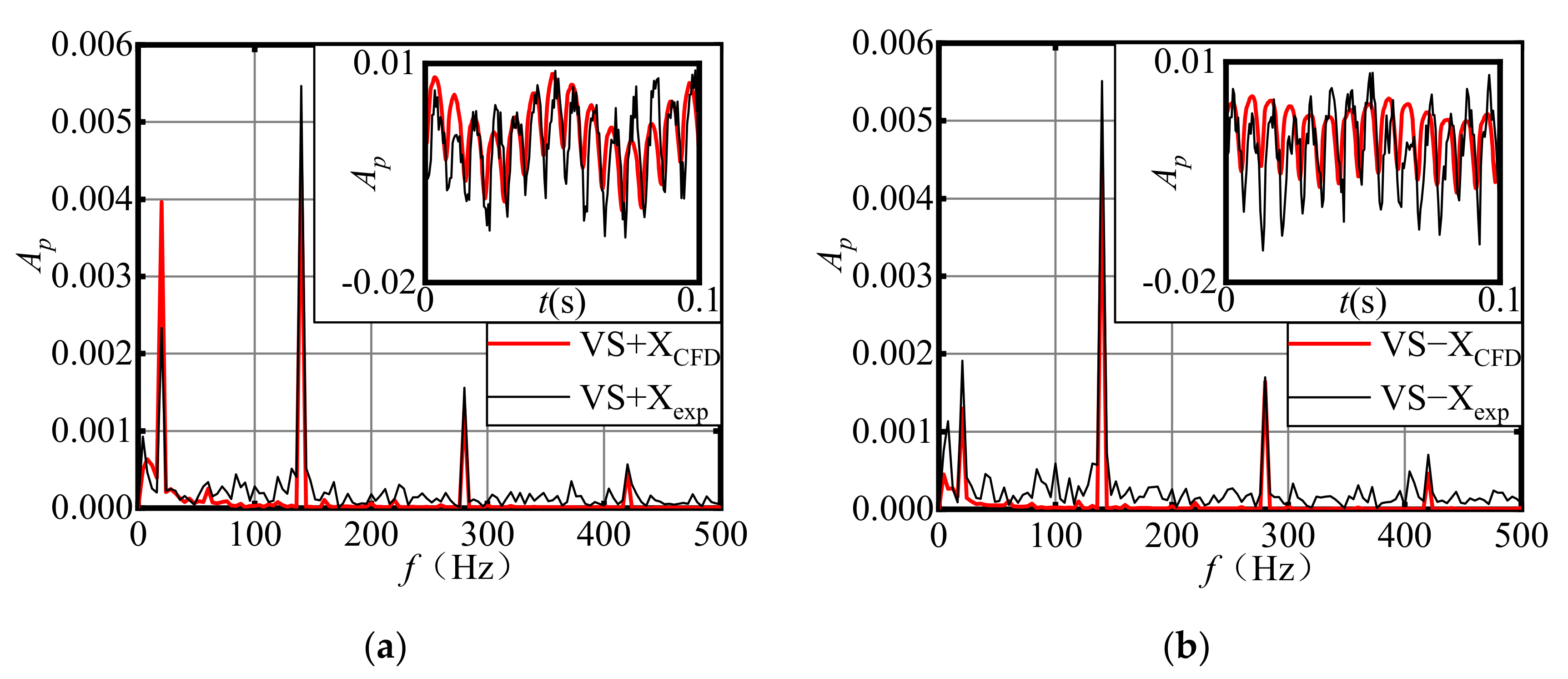
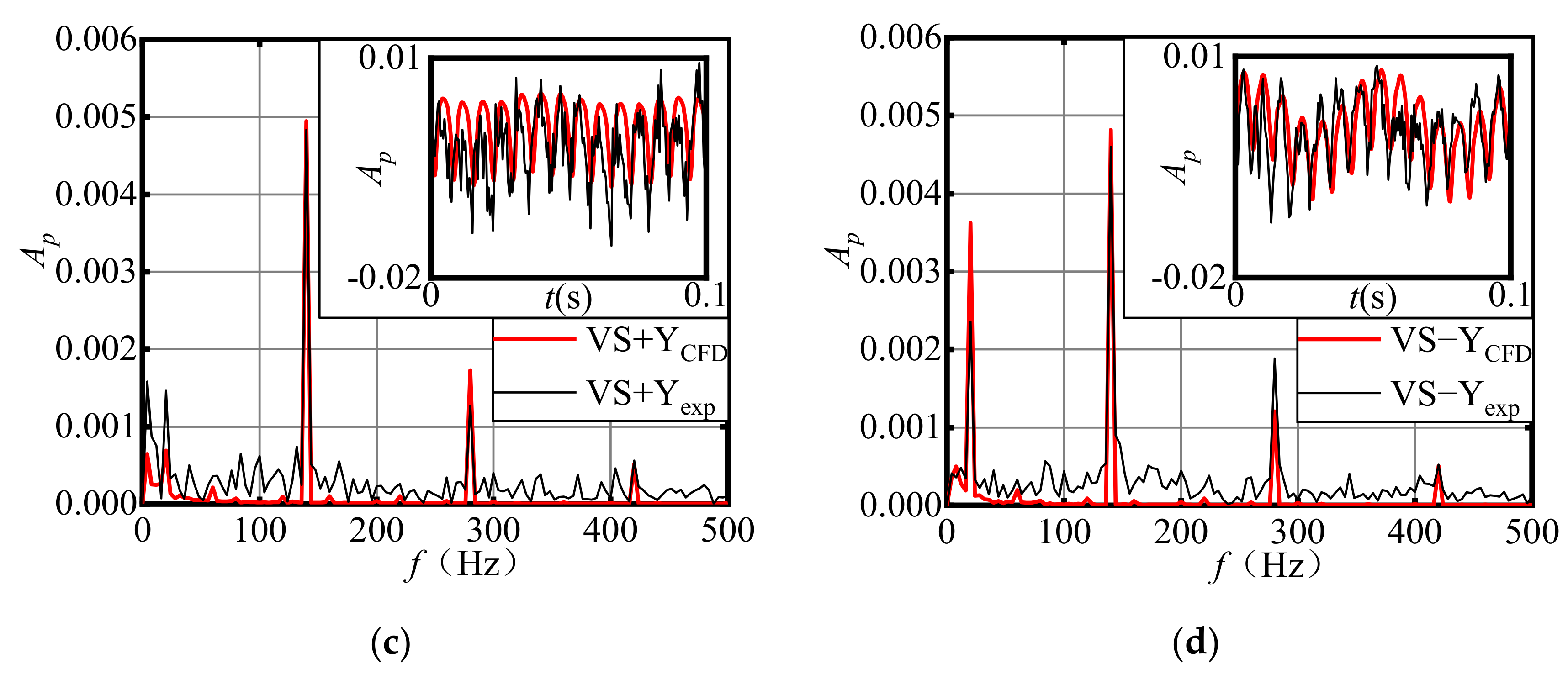
3.7. Experimental-Numerical Verification

For the accuracy of the numerical simulation results, validation is necessary to compare CFD and experimental data. The head versus the flow rate curve and the efficiency versus the flow rate curve are shown in Figure 9. Highly matched results of CFD and the experiment can be observed, especially around the design point that φ = φ d . The efficiency at φ d is higher than 90%, which shows a good hydraulic performance. The gap between the experimental and numerical values of efficiency at φ d is 0.1%, and the gap between the experimental and numerical values of the head at φ d is 5.2%.
The comparisons of frequency-domain and time-domain of pressure fluctuation between the experiment and CFD results at φ d are shown in Figure 10. The frequency resolution is 4 Hz. FFT is used for the time-frequency analysis without the windowing and weighing function. Among them, the time-domain diagram is obtained by taking three impeller revolutions into consideration. Both the time-domain and frequency-domain data were found accurate especially in capturing the blade-excited frequencies. The one time, two times and three times of BPF were well simulated out. Therefore, the CFD simulation was accurate and reliable enough in the analyses below.

4. Result and Discussion

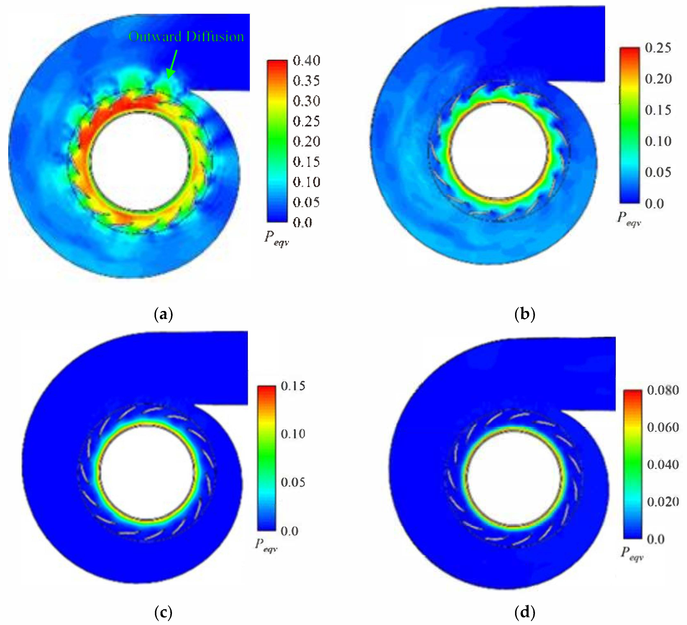
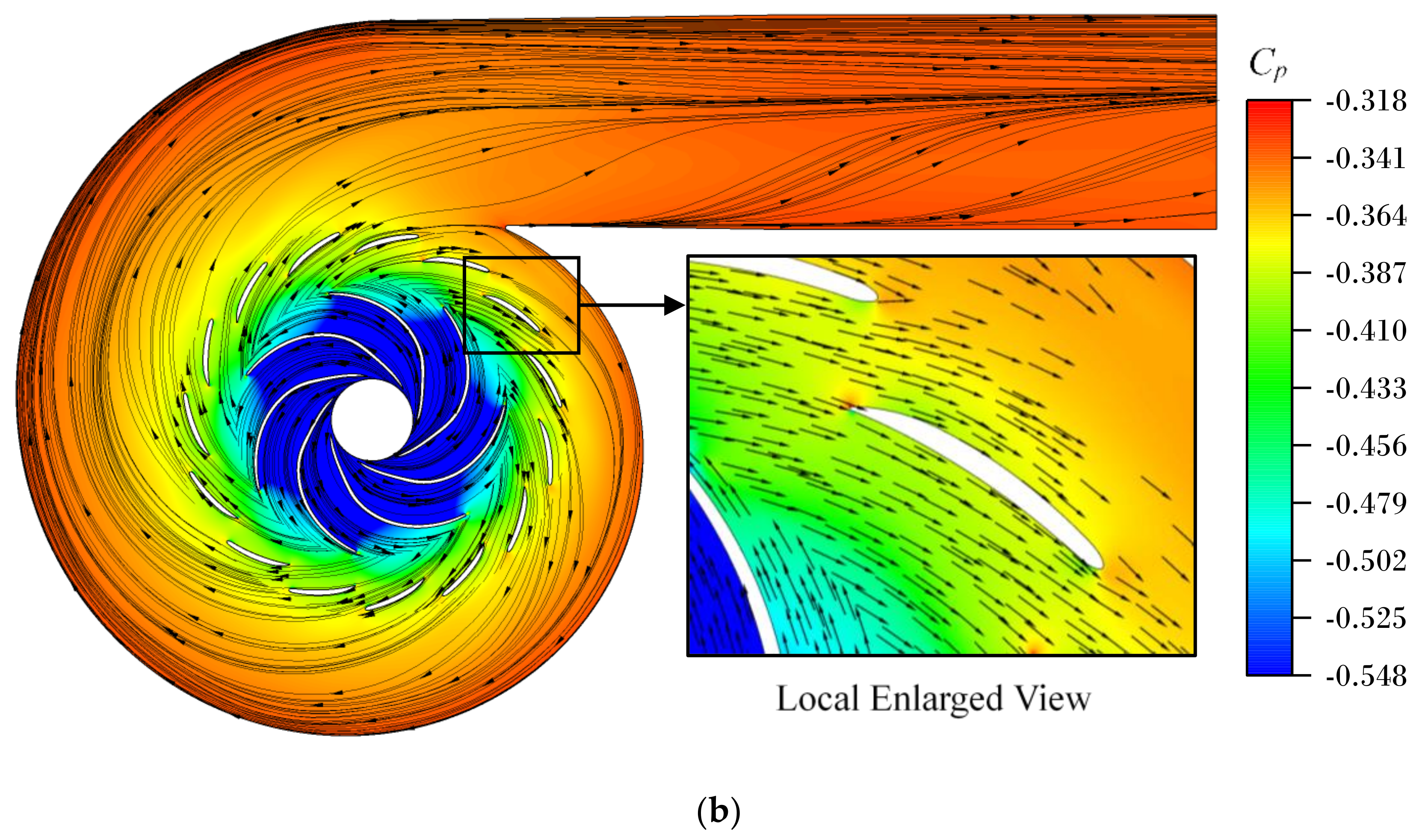
4.1. Pressure Contour and Velocity Vectors

To understand the pressure pulsation in the vaneless region, it is necessary to have an overview of the local flow pattern in the pump. Figure 11 shows the pressure contour and velocity vectors at φ d condition on the Z = 0 plane and impeller mid-span surface. Local flow regime is smooth without obvious vorticial structures. C p globally increases along the streamwise direction. Fluid gets both kinetic and pressure energy well from impeller. Then, the kinetic energy is well converted into pressure energy when flow passes through the diffusers. There are local high-pressure sites in front and local low-pressure sites on the back of the vaned diffuser leading-edge. At the leading-edge of the vaned diffuser, obvious flow separation can be found, which is the main reason why pressure suddenly varies. In detail, the flow striking causes local high pressure, and the flow separation causes local low pressure.

4.2. Pressure Pulsation at Scatter Points in Vaned Diffuser

To study the characteristics of pressure pulsation, four monitoring points were added in the vaneless region and the middle of the vaned diffuser passage along the flow (streamwise) direction on the Z = 0 plane. The distributions of added points Pa1~Pa4 are shown in Figure 3. Pa1 was located in the middle of the vaneless region. Pa2, Pa3, and Pa4 were orderly distributed in the vaned diffuser channel from leading edge to trailing edge. The time resolution was 6.944 × 10⁻⁵ s and the frequency resolution was 4 Hz. The time-frequency characteristic diagram is shown in Figure 12.
As shown in Figure 12, the main amplitude in the vaneless region and between the vaned diffuser is a narrow band frequency of 140 Hz, which is 7 (impeller blade number) times that of the impeller frequency. Along the flow direction, the amplitude of the BPF gradually decreases, and the second and third harmonics of the BPF rapidly decrease and disappear, while other frequencies are basically unchanged. The amplitude of BPF decreases and is lower than the amplitude of impeller frequency. In the whole process, there is always a low frequency broadband. There is a low frequency band of about 60 Hz between the vaneless region and vaned diffuser. It disappears in the volute.
In the vaneless region, BPF with a high amplitude is dominant in affecting pressure pulsation. As shown in Figure 12, the amplitude of BPF attenuates rapidly along streamwise direction. This is mainly because the working condition is a design point working condition, and the flow pattern is smooth without an obviously vorticial flow or flow separation. Moreover, there is always a broadband between 0–20 Hz and the rotation frequency is 20 Hz.
In this paper, the main research object was the source, the propagation, and the attenuation law of the amplitude of BPF. Therefore, a tracking of the BPF is supplied in a perspective of innovation in the following sections.

4.3. Tracking and Visualizing of Pressure Pulsation in Diffusers

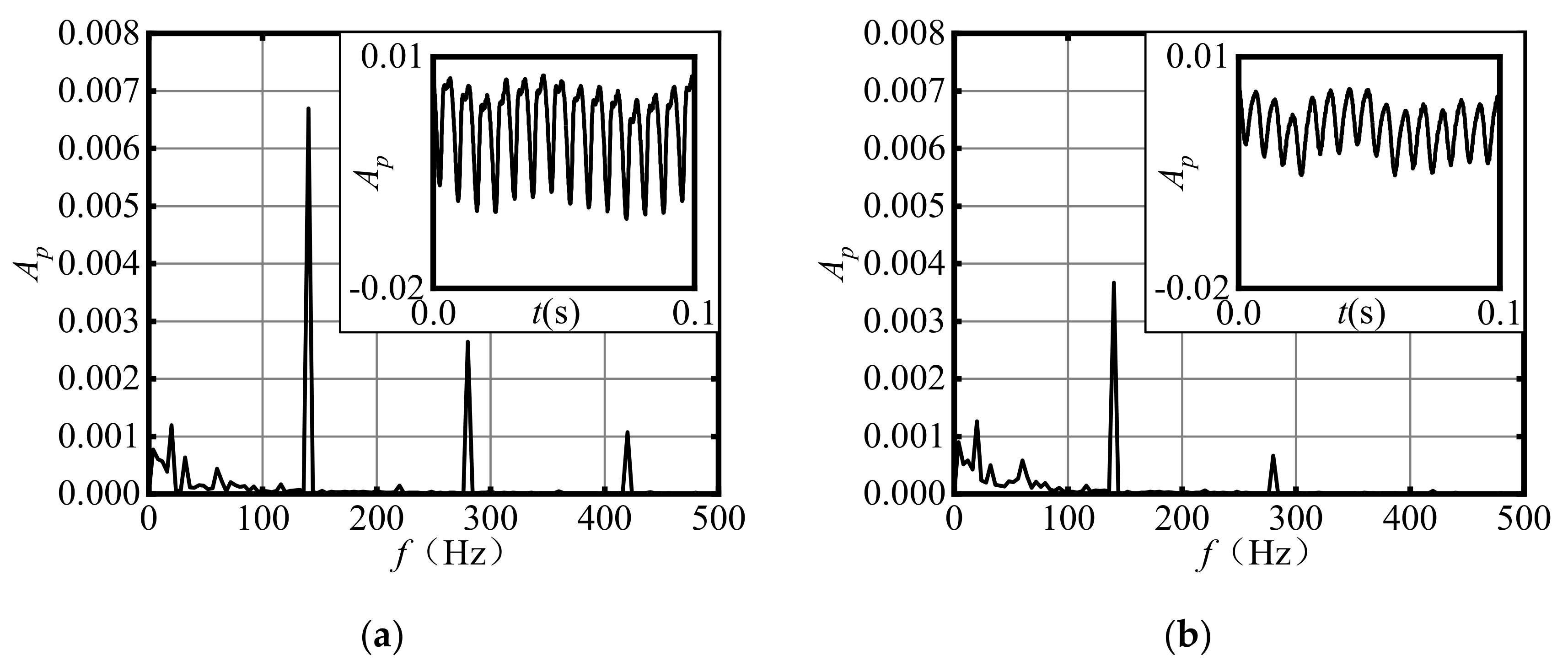
4.3.1. Main Frequency

Main frequency is an important quantity in frequency-domain analysis. It represents the dominant frequency in a certain signal. Figure 13 shows the main frequency distribution on Z = 0 plane in diffusers. In the vaneless region and vaned diffuser, the main frequency is BPF of 140 Hz and its harmonics. Along the streamwise direction in the vaned diffuser, main frequency gradually changes from BPF to the impeller frequency of 20 Hz. Based on the BPF part with green color as shown in Figure 13, there is an obvious outward diffusion phenomenon of BPF along the radial direction with the volute section area growing.

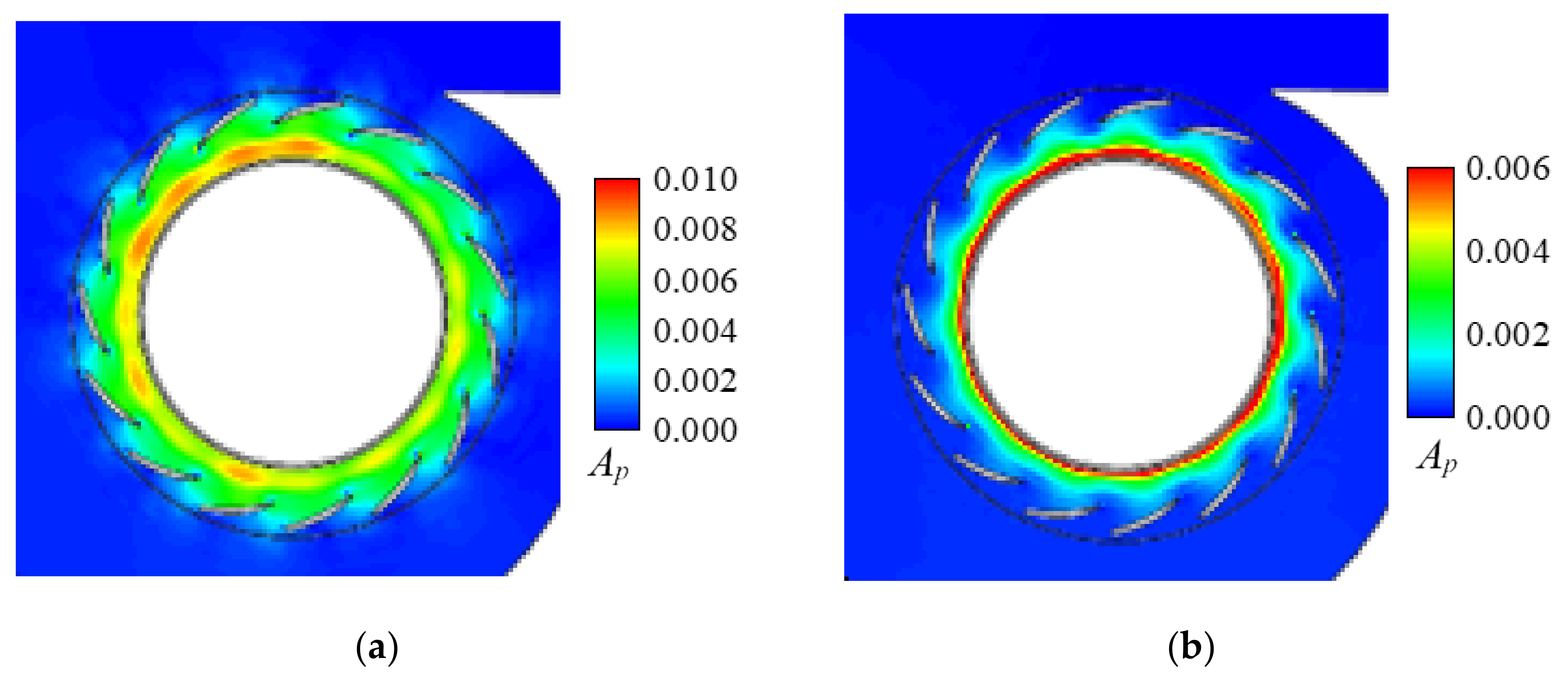
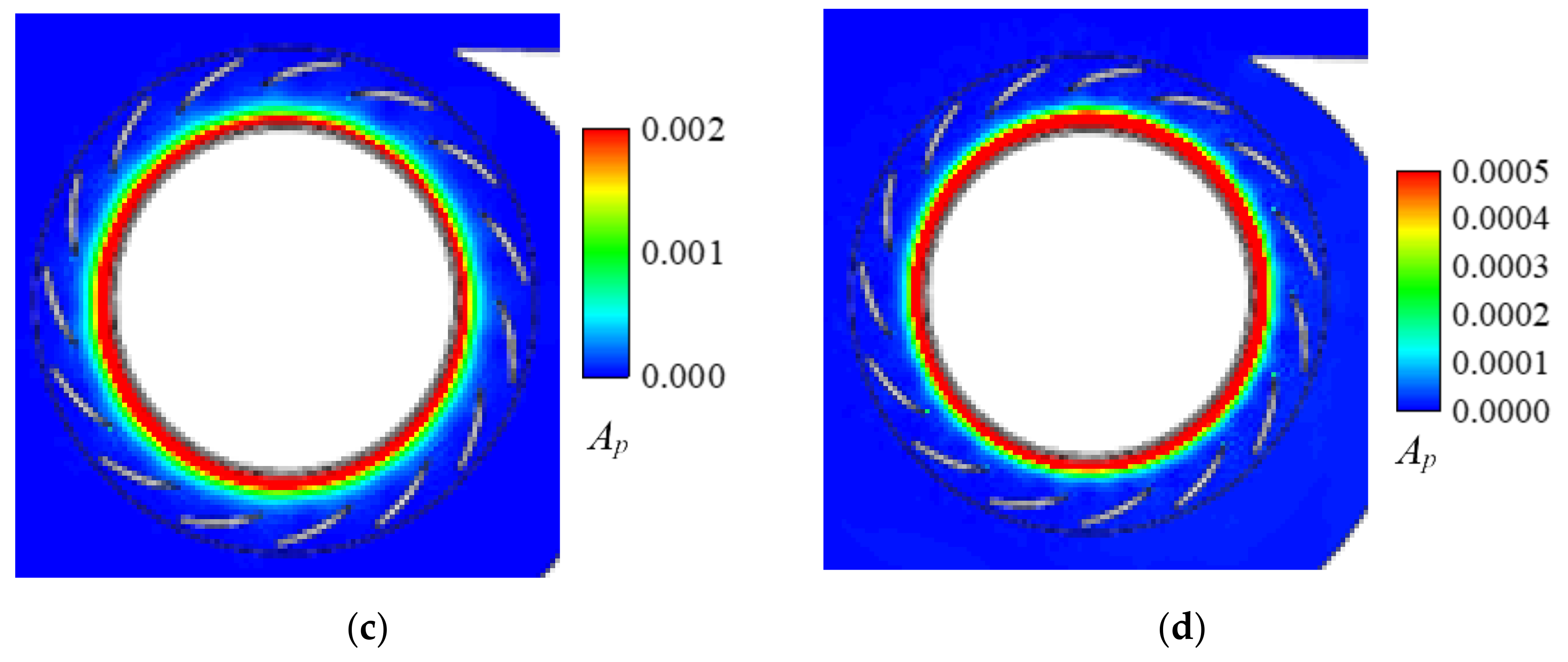
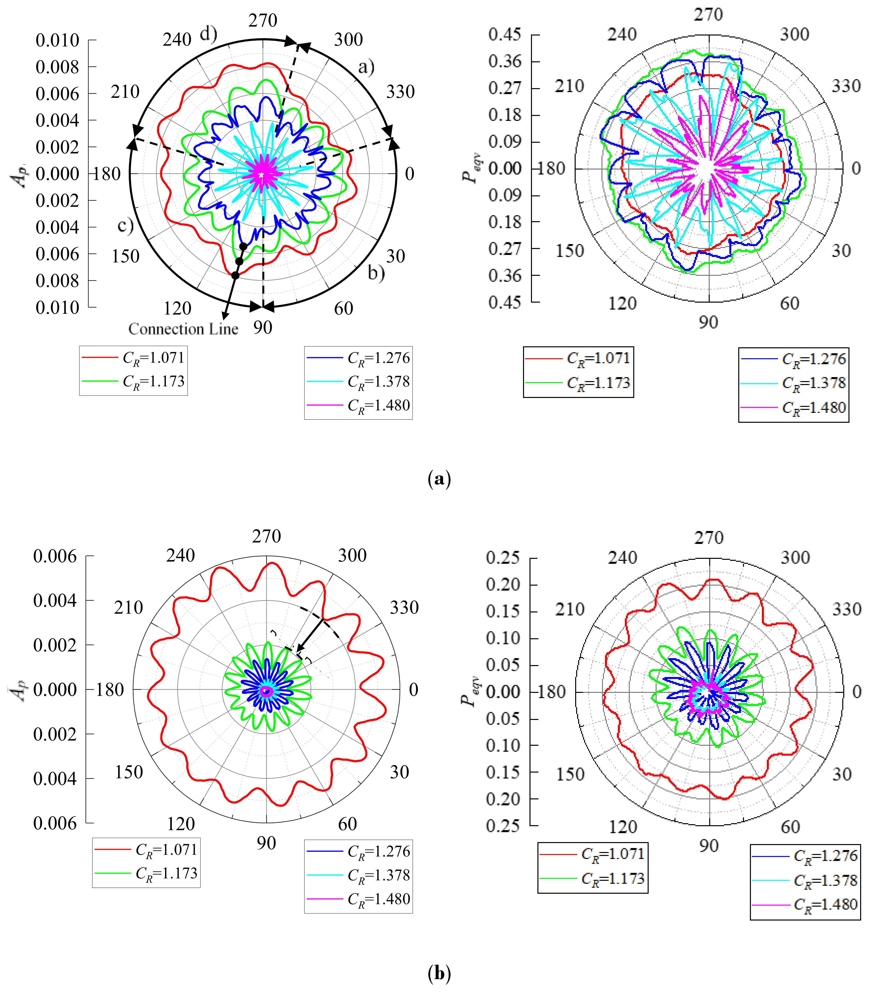
4.3.2. Absolute and Relative Amplitude of Typical Frequencies

The amplitude of pressure pulsation is an important parameter in this case. Based on Figure 10 and Figure 12, there are typical frequencies that are the impeller frequency 20 Hz, BPF 140 Hz, and the second, third, and fourth harmonics of BPF 280 Hz, 420 Hz, and 560 Hz. The absolute amplitude of BPF and its harmonics is analyzed by comparing the Ap contour on the Z = 0 plane in Figure 14.
The BPF and its harmonics strongly vary in diffusers as shown in Figure 14a–d. In the vaneless region, the amplitude of BPF and its harmonics gradually decreases. Among all the blade-excited frequencies, a higher frequency has a shorter propagation distance. The highest amplitude region of BPF is located in the middle of the vaneless region instead of close to the impeller blade’s trailing edge. However, the highest amplitude region of the other BPF’s harmonics is very close to the impeller blade’s trailing-edge position. The amplitude in the vaned diffuser and the vaneless region is obviously higher than that behind the vaned diffuser.

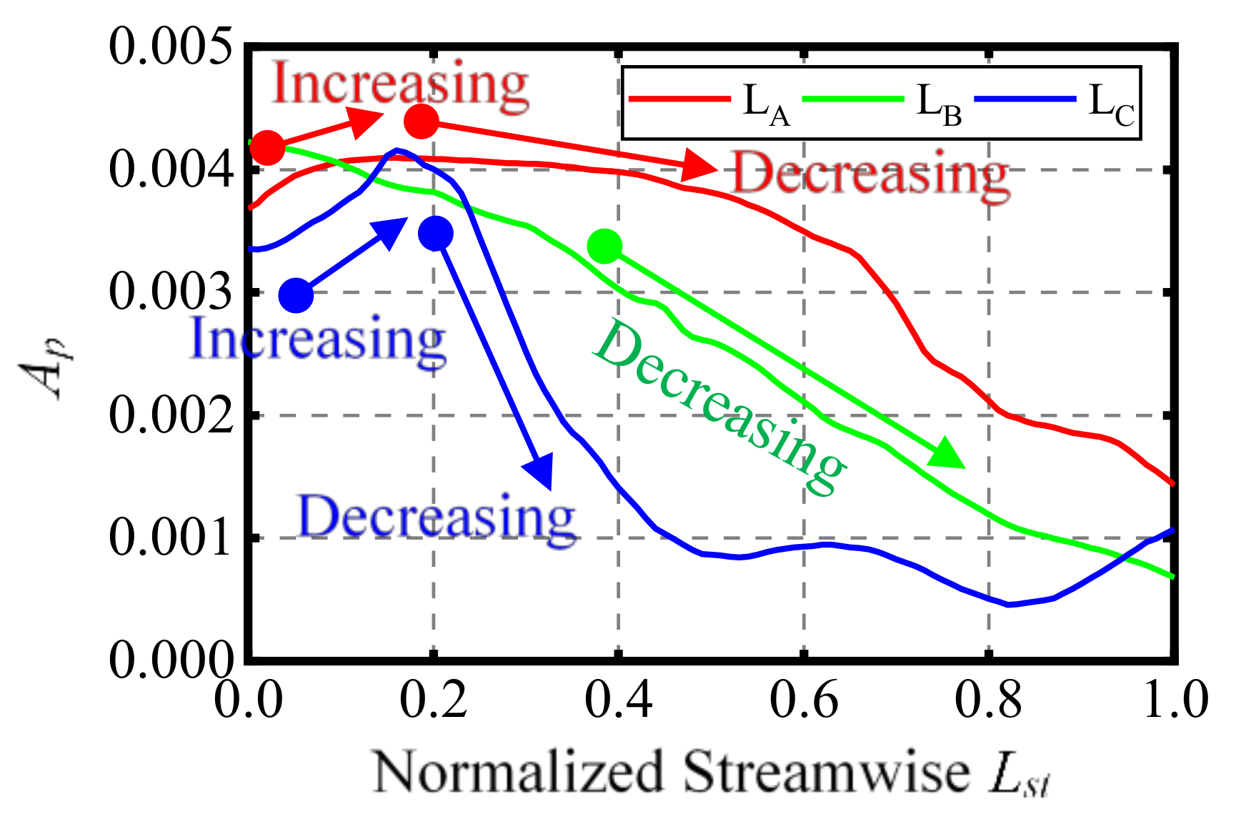
4.3.3. Relative Amplitude of Typical Frequencies

Compared with the absolute amplitude, the relative amplitude will perform better in tracking the spatial propagation and distribution of a specific frequency. Thus, parameter P e q v is defined to show the relative amplitude:
P e q v = p p max p min
where p is the pressure at a certain point and a certain time, and p max and p min are the maximum and minimum pressures at this certain point. This parameter is the purity of main frequency, which eliminates the influence of its own strength. Larger P e q v is, higher than the proportion of frequency is. It is accurate in judging the pressure amplitude change of a certain frequency.
Figure 15 shows the distribution of the purity P e q v on the Z = 0 plane. Figure 15a–d are the P e q v contours of BPF and its harmonics. The P e q v contour shows the blade-excited frequency series better in the vaneless region. High order harmonics of BPF dominate the region close to the impeller trailing edge. Low order harmonics of BPF dominate the middle of the vaneless region. BPF dominates the vaned diffuser channel. Outward diffusion patterns can be seen in the contour of BPF. The variation law of P e q v contour shows that the impeller blade generates complex high-order BPF harmonics. When flow deviates away from the impeller and is interrupted by the vane, high order harmonics interact on each other to enhance lower-order BPF characters. The high amplitude region in the vaneless region is wider where the volute section-area is larger along the spiral direction. It shows that the high amplitude range in the vaneless region is affected by the volute.

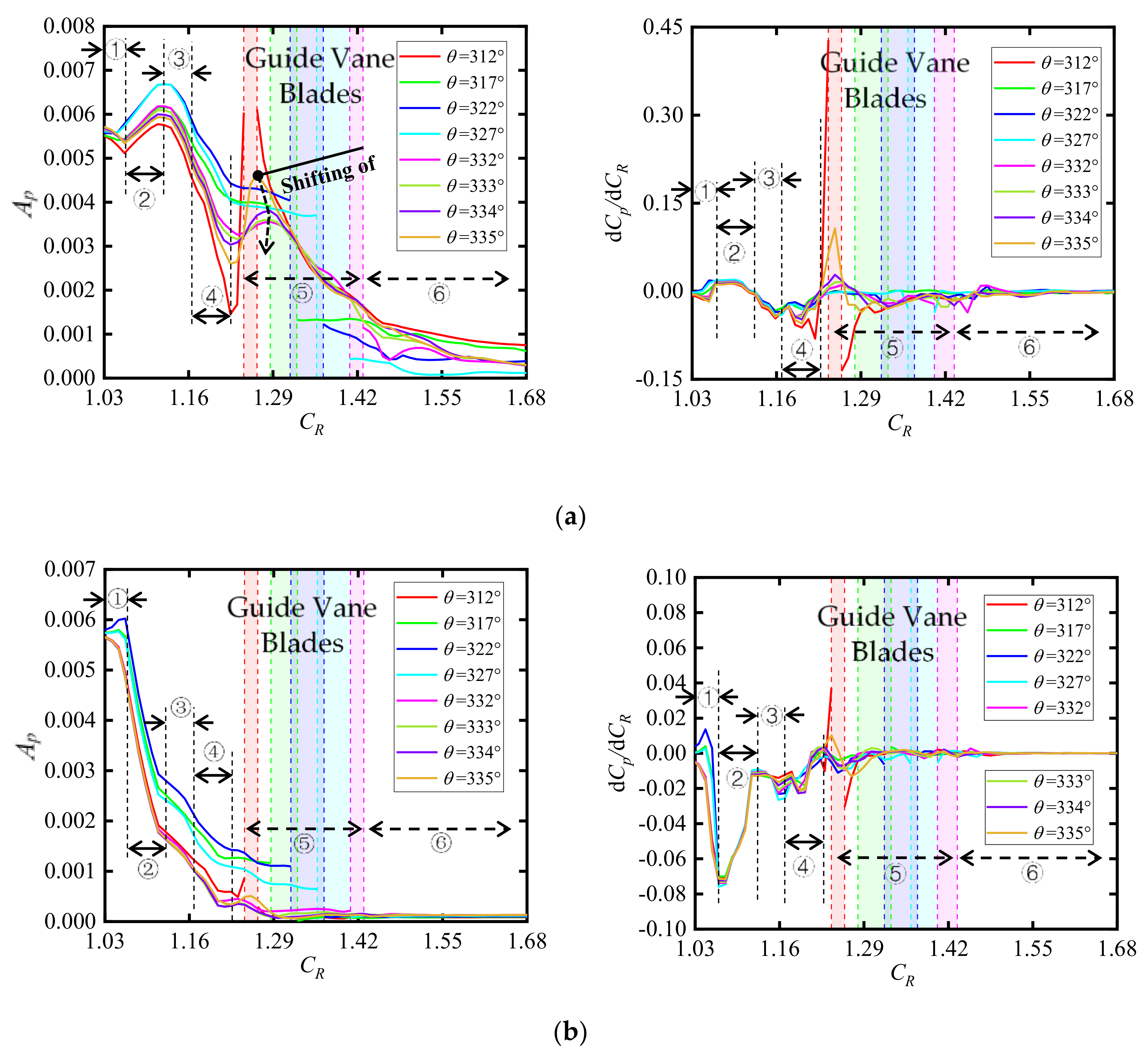
4.3.4. Detailed Distributions of Pressure Pulsation amplitudes

The A p contour and P e q v contour provide a good spatial visualization of pressure pulsation. However, more detailed information is required, especially for the local sudden change of pressure pulsation amplitudes. Thus, reference angle and positions are defined to have a better analysis on the Z = 0 plane. Considering the different radius position r, the dimensionless radius C R is defined as:
C R = r R iout  
Figure 16 shows the reference angle and positions. The circumferential angle θ is defined along the impeller rotation direction ω. Three streamwise lines LA, LB, and LC are set in a vaned diffuser channel that is dominated by 60 Hz frequency. Five ISO- C R circles are set within C R = 1.071~1.480. Five ISO-θ lines are set at every 5 degrees within θ = 312~332 degrees. After the θ = 332 degrees’ line, three ISO-θ lines are set at every 1 degree within θ = 333~335 degrees as a refinement. Therefore, the absolute amplitude A p and relative amplitude P e q v of typical frequencies are analyzed in Figure 17, Figure 18 and Figure 19.
The absolute amplitude A p and relative amplitude P e q v on the ISO- C R circles from θ = 0 degree to 360 degrees are shown in Figure 17. Figure 17a,b are about the BPF and its second harmonic frequency. The circumferential variation law of A p and P e q v are similar. In total, 15 (vaned diffuser blade number) periods can be seen at different C R positions. For example, for A p of BPF, the amplitude increases with the increasing volute section-area. The phenomenon becomes stronger when the C R is smaller. The circumferential fluctuation period can be divided into four parts along θ direction that are (a) 285–345 degrees, (b) 345–90 degrees, (c) 90–195 degrees, and (d) 195–285 degrees. In each part, the local peak and valley are at the same level. It shows that the volute not only affects amplitude distribution range, but it also affects the maximum value of amplitude, and the volute cut-water especially has great influence, which causes the sudden decrease of amplitude. The vaned diffuser geometry also affects the A p amplitude distribution that the peak corresponds to mid-channel when the valley is near the blade leading-edge. There is a special phenomenon at the three radial positions that are C R = 1.071, 1.173, and 1.276, which are upstream from the vaned diffuser. Their peak and valley positions strongly overlap in circumferential direction with the connection line (as indicated) perfectly towards the radial direction. It reveals the radial propagation of pressure pulsation in the vaneless region. At the radial position that C R = 1.378, the local peak is still high with the valley becoming very low. The maintaining high peaks are because of the accumulation phenomenon of pressure pulsation on the vaned diffuser blade concave side. At C R = 1.480, both the peaks and valleys strongly drop to a lower level. This is because C R = 1.480 circle is on the convex side of the blade, which is out of the accumulation region. In general, the maximum A p amplitude level decreases from about 0.008 to about 0.0015 along the radial direction. For BPF, the P e q v curves are similar to the A p curves but with an amplification that all the distribution laws are much clearer. The distribution laws A p and P e q v amplitudes of the second harmonics of BPF are similar to that of BPF. The positions of peaks and valleys still correspond to the vaned diffuser. However, it is not obviously affected by the volute. The A p and P e q v amplitude levels are stable along the circumferential direction. The amplitude of second harmonics of BPF has a rapid drop from C R = 1.071 to 1.173 as indicated. It drops by at least 0.002, which is approximately 0.3% of the pump head.
Because some specific pressure pulsation propagations are found along the radial direction, it is necessary to have detailed analyses along the radial reference lines. As the pressure wave can pass through objects, the radial distributions, especially across blades, can indicate special variations. To understand the detailed radial variation laws, the absolute amplitude A p on the ISO-θ lines from C R = 1.03 to 1.68 are shown in Figure 18. To have more direct results of the attenuation of typical frequencies, the derivative of A p against C R is also plotted as d A p /d C R .
Figure 18a,b are the radial distribution of A p and d A p /d C R of BPF and its second harmonic frequency. Their variation laws are very complex. For a better comparison, six different regions are divided as shown in Figure 18a,b. They are, respectively, named ① impeller blade trailing-edge downstream region, ② amplitude fluctuation region, ③ vaneless attenuation region, ④ pre-guide-vane fluctuating region, ⑤ inter-channel attenuation region, and ⑥ post-guide-vane attenuation region. The ① impeller blade trailing-edge region is near the impeller blade trailing-edge. It is a complex region where both the A p of BPF and the second harmonic of BPF are strong, about 0.0055~0.0058. Different θ positions have different variation tendencies. For example, the θ = 327 degrees’ site is near one of the peaks in Figure 17a,b. The A p of BPF and the second harmonic of BPF may rise locally. On the contrary, the θ = 335 degrees’ site is near one of the valleys in Figure 17a,b. The A p of BPF and the second harmonic of BPF may decrease locally. In the figures d A p /d C R , both positive and negative values can be found in region ①. The ② amplitude fluctuation region, ③ vaneless attenuation region, and ④ pre-guide-vane fluctuating region are in the middle of the vaneless region. In the ② amplitude fluctuation region, BPF suddenly changes from decreasing to increasing, but the second harmonic of BPF still keeps r A p idly decreasing. The d A p /d C R values of BPF are positive, and that of the second harmonic of BPF is negative. It may indicate the interaction and transmission of pressure pulsation amplitude from the second harmonic of BPF to BPF. Along the radial direction, the BPF’s A p increases slower with the quicker attenuation of 2BPF’s A p when the 2BPF’s A p becomes very low. This is also why the maximum A p of BPF is in the middle of the vaneless region instead of near the impeller trailing edge. In the ③ vaneless attenuation region, the A p of both BPF and the second harmonic of BPF decreases. The values of d A p /d C R are negative for BPF and the second harmonic of BPF, which indicates an accelerated attenuation in this region. However, for the second harmonic of BPF, the attenuation becomes slower than that in the ② region. The ④ pre-guide-vane fluctuating region is slightly similar to the ③ region because A p is also locally decreasing. However, it is different because d A p /d C R is fluctuating in the ④ region. It indicates a very complex local flow pulsation due to the influence of the vaned diffuser. The ⑤ inter-channel attenuation region is in the vaned diffuser channel near the blade concave surface. There are two different typical conditions. First, near one of the peaks in Figure 17a,b, the A p attenuates stably and flatly with a low level in the ⑤ region because of the prevention effect of the vaned diffuser blade. Second, near the leading edge of the vaned diffuser, the A p is rapidly rising and then suddenly decreasing down with a local peak. There is a spatial shifting phenomenon of local peaks that can be indicated on the C R - A p figure. With the decreasing of θ, for example, from 335 to 332 degrees, the propagation direction shifts from one blade leading edge to the upstream blade’s concave surface. It indicates the deflection of the pressure wave under the influence of the vaned diffuser leading edge. The ⑥ post-guide-vane attenuation region is downstream to the vaned diffuser from the blade convex side to the volute. The A p in this region attenuates slower and slower. The A p of the second harmonic of BPF decreases to a very low level. The value of d A p /d C R is at a small negative level. It indicates the slow attenuation of pressure pulsation amplitude without the vaned diffuser’s interference.
The variation of A p on the streamwise lines is also important for understanding the pressure pulsation propagation in the vaned diffuser channels. The streamwise length is normalized into L s t = 0~1, as shown in Figure 19. As illustrated in Figure 16, LA is the streamwise line on the blade concave side, and LC is the streamwise line on the blade convex side. The A p on the two lines are similar as there is a local increasing and decreasing around the blade leading-edge. It shows the importance of the leading-edge geometry again in affecting pressure pulsation. As illustrated in Figure 16, LB is in the mid-channel, which is relatively far away from the leading edge. Therefore, A p continually decreases on LB from L s t = 0 to L s t = 1.
The vaned diffuser blade, especially the leading edge, has a strong effect on pressure pulsation. BPF and its harmonics are found interacting with each other on local strong amplitude variations. The attenuation and propagation laws of pressure pulsation amplitude are somehow indicated, which provides a new understanding of pulsation flow driven by rotor-stator interaction in the vaneless region, vane channels, and downstream diffusers.

4.3.5. Phase and Phase Difference

The initial phase is important to analyze phase and phase difference. In this study, it is defined at the volute cut-water. Figure 20 shows the distributions of phase difference of typical frequencies on the Z = 0 plane. As the sine and cosine functions are the basis functions in Fourier transform, the phase will change within -π to π. If the phase difference is π, which is called antiphase, all the temporal states, including displacement, velocity, and acceleration, are completely on the contrary. If the phase difference is 0 or 2π, all the temporal states are in the same status. Phase π and −π in Figure 20 is also the same. Due to the interpolation problem, mutations can be seen between adjacent π and −π, which are smooth transitions.
Figure 20a–d shows the phase difference of BPF and its harmonics. In the vaneless region, the pattern of phase difference is strongly periodic. The number of periods relates to the impeller blade number. For example, 140 Hz frequency (BPF), 280 Hz frequency, 420 Hz frequency, and 560 Hz frequency have respectively 7, 14, 2,1 and 28 periods. Without the interference of vane blades, the pressure wave fluctuates along the circumferential direction repeating the same states. This means that the BPF and its harmonics in the vaneless region are only influenced by the impeller, and the impeller influences the BPF and its harmonics mainly in the circumferential direction. The BPF and its harmonics propagate along the radial direction. The vaned diffuser, especially the leading edge, interferes with the propagation of pressure wave and broke the circumferential phase fluctuation pattern. In a single vaned diffuser channel, the phase is almost the same. As pressure wave propagates along the radial direction, the circumferential phase fluctuation pattern is outward diffusing from the vaned diffuser to the volute with diffraction patterns. The lower the order the harmonic of BPF is, the further it diffuses. This means in the outlet of the vaned diffusers, as indicated in Figure 20a, the outward diffusion of BPF is obvious. On the contrary, as shown in Figure 20d, the circumferential phase fluctuation pattern of four times of BPF stops on the vaned diffuser leading edge. The volute cut-water is important in affecting the pressure wave propagation. As indicated in Figure 20a, the outward diffusion of BPF is fluctuating between −0.5π to −π. The two times and four times of BPF have also a phase change from 0 to −π there. In the volute straight section, the phase difference pattern is divided into three parts, as indicated by upper, middle, and lower. The upper and lower part have the same phase. The middle part has the phase with a difference of π with the upper and lower parts. This three-part pattern is related to the local merging flow in the volute straight section, as shown in Figure 11. Phase differences can be found among different frequencies.
The spatial distribution of phase well indicates the trend and state of BPF and its harmonics’ pressure variations. As shown in Figure 20a, the phase difference between adjacent vane channels is about π, which means that the pressure change between adjacent vanes channels is completely opposite. Similarly, at the outlet of the vaned diffusers, the diffraction fringes indicate that there is variable pressure change. However, it has little effect because the amplitude of BPF at the outlet is not strong. It is difficult to observe these phenomena by conventional methods.

4.4. Discussions

According to the PTN-based analyses above, there are some discussions for a better summary of the tracked pulsation characters. Figure 21 is drawn for detailed illustrations. The pulsation amplitude is found alternatively weak and strong in the vaneless region. As the blade-excited pressure wave propagates along the radial direction, this alternative amplitude pattern indicates the interference of the vaned diffuser on pressure pulsation amplitude. Based on the PTN analysis, it is always weaker for the amplitude of BPF near the vaned diffuser leading edge in the vaneless region due to the vaned diffuser blocking effect. It is always stronger for the amplitude of BPF near the vaned diffuser mid-channel.
Vaned diffuser geometry has two main influences that are deviation and accumulation on pressure pulsation propagation. As the vaned diffuser is designed for flow guidance, the radial flow from the impeller is guided into a more circumferential direction for downstream volute. Leading edge, which is the site nearest to the impeller, may deviate flow onto the concave side of the adjacent vane blade. This why a deviation can be found on the connection of pulsation amplitude peaks in the vaned diffuser channel. At the same time, the blade concave side prevents the deviated flow. The accumulation effect can be found on the vane blade concave side with local strong pressure pulsation amplitude. Similar effects can be found at the volute cut-water, which can be treated as a single vane. It also strongly affects the pressure pulsation. Therefore, the impeller is the main source of pulsating signal, and the vaned diffuser enhances pulsation amplitude in the local region, especially near the head of blade. Then, the pulsation amplitude attenuates quickly in the vaned diffuser channel.
Overall, pressure pulsation amplitude generally attenuates in the vaned diffuser. In the vaneless region, the BPF series frequencies rapidly attenuate but with BPF local enhancements due to the influence on each other. High order harmonics of BPF attenuate earlier. Low order harmonics such as BPF and two times BPF may shortly self-enhance by receiving the energy from attenuated high-order harmonics. As the vaned diffuser geometry has the obstruction effect on the pressure wave, the pressure pulsation amplitude attenuates slower, which even increases near the vane blade, especially at the leading edge. However, there is a small region with low amplitude at the leading edge of blade. There is a high pressure and a low flow velocity region in the front of the blade leading edge because of the impact between flow and the leading edge. In this region, the pressure pulsation is stable and with low amplitude. The closer to vane blade concave side, the slower the attenuation is, but at the convex side, the amplitude attenuates rapidly. The amplitude attenuates to a lower level. After the pressure wave bypasses the vaned diffuser, the amplitude attenuation decelerates without strong preventions. Hence, the vaned diffuser made the amplitude of the pulsating signal attenuate overall.
The spatial distribution of phase difference is interesting. Phase change from π to 0 to −π indicates a complete waveform and sub-flow of a certain frequency. In the vaneless region, BPF and its harmonics have several complete waveform periods along the circumferential direction. It indicates the circumferential sub-flow in the vaneless region. However, there are some local incomplete phase changes. For example, the phase of BPF fluctuates between −0.5π to −π near the volute cut-water. The composition of the pattern is two or more sub-flow that have similar frequencies, but different directions, interfere with each other and mix, and then they result in a phenomenon such as wave interference.
Vaneless region, guide vaned diffuser, impeller blades and vaned diffuser blades have obvious influences on the propagation characteristics of BPF and its harmonics based on the above analysis. The vaneless region can be enlarged for the amplitude rapid attenuation when designing the pump, and close attention must be paid to the head and the blade angle at the medium of the vaned diffuser blade to avoid the enhancement of pressure pulsation amplitude.

5. Conclusions

In this study, the propagation and attenuation of pressure pulsation in the diffusers of large-scale vaned-voluted centrifugal pumps were numerically tracked and visualized. The experiment verifies the accuracy of the simulation. Conclusions can be drawn as follows:
(1)
When a large-scale vaned-voluted centrifugal pump is operating at design-load, impeller frequency and blade-excited frequency are the pressure pulsations dominant in diffusers. The impeller frequency of 20 Hz, the blade passing frequency (BPF) of 140 Hz, and its high order harmonics that are 280 Hz, 420 Hz, and 560 Hz can be obviously found. By analyzing the variation law of pressure pulsation in one vaned diffuser channel, attenuations of the BPF and BPF’s harmonics are found along the streamwise direction.
(2)
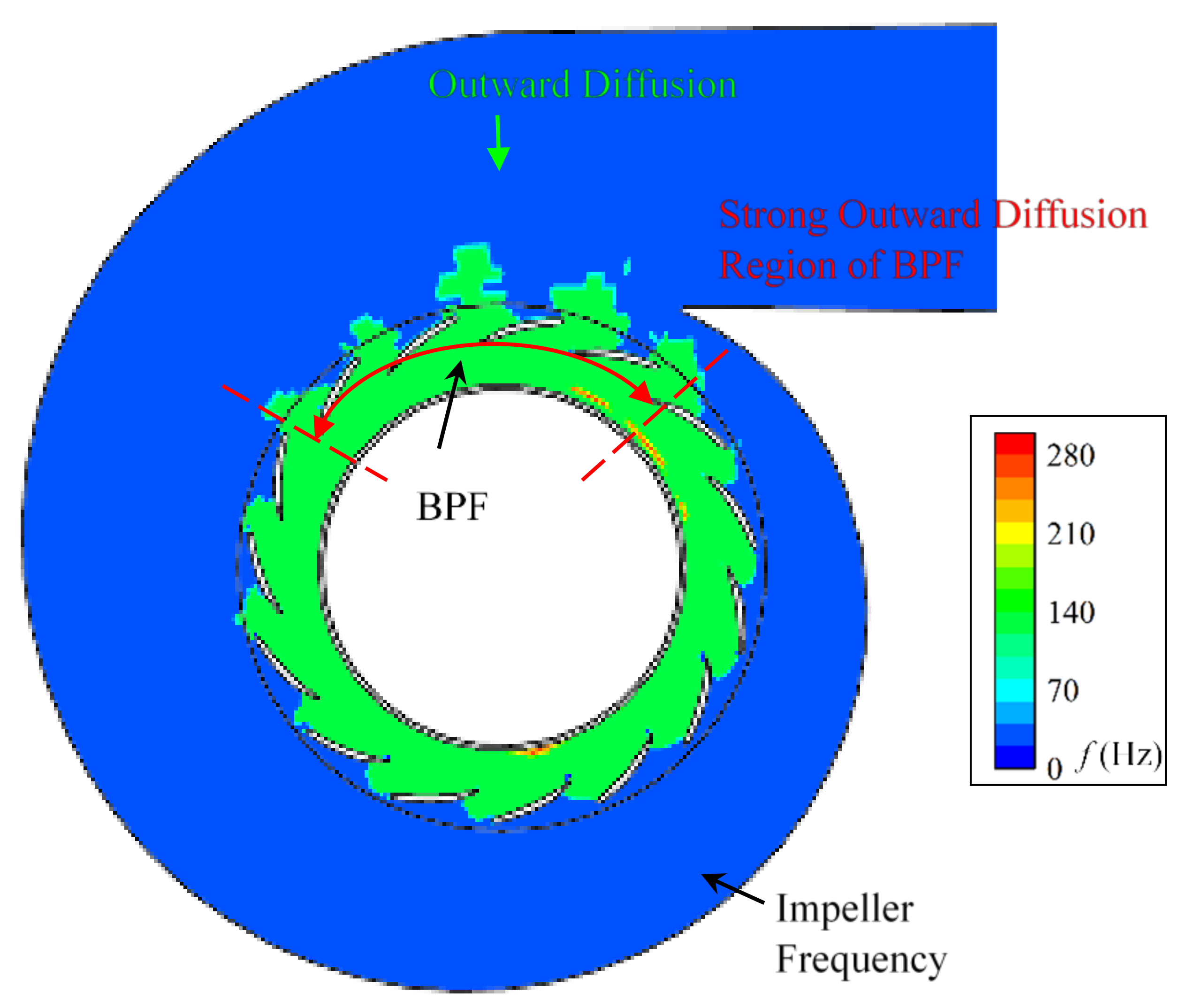
By using the pulsation tracking network (PTN), it is possible to have a more detailed visualization of the source, propagation law, and attenuation law of pulsation frequencies. The BPF series are obviously related to the impeller and vaned diffuser. The BPF series is concentrated in the vaneless region and the inlet of the vaned diffuser channel. The significant influence region and amplitude of BPF have a positive correlation with the sectional area of the volute.
(3)
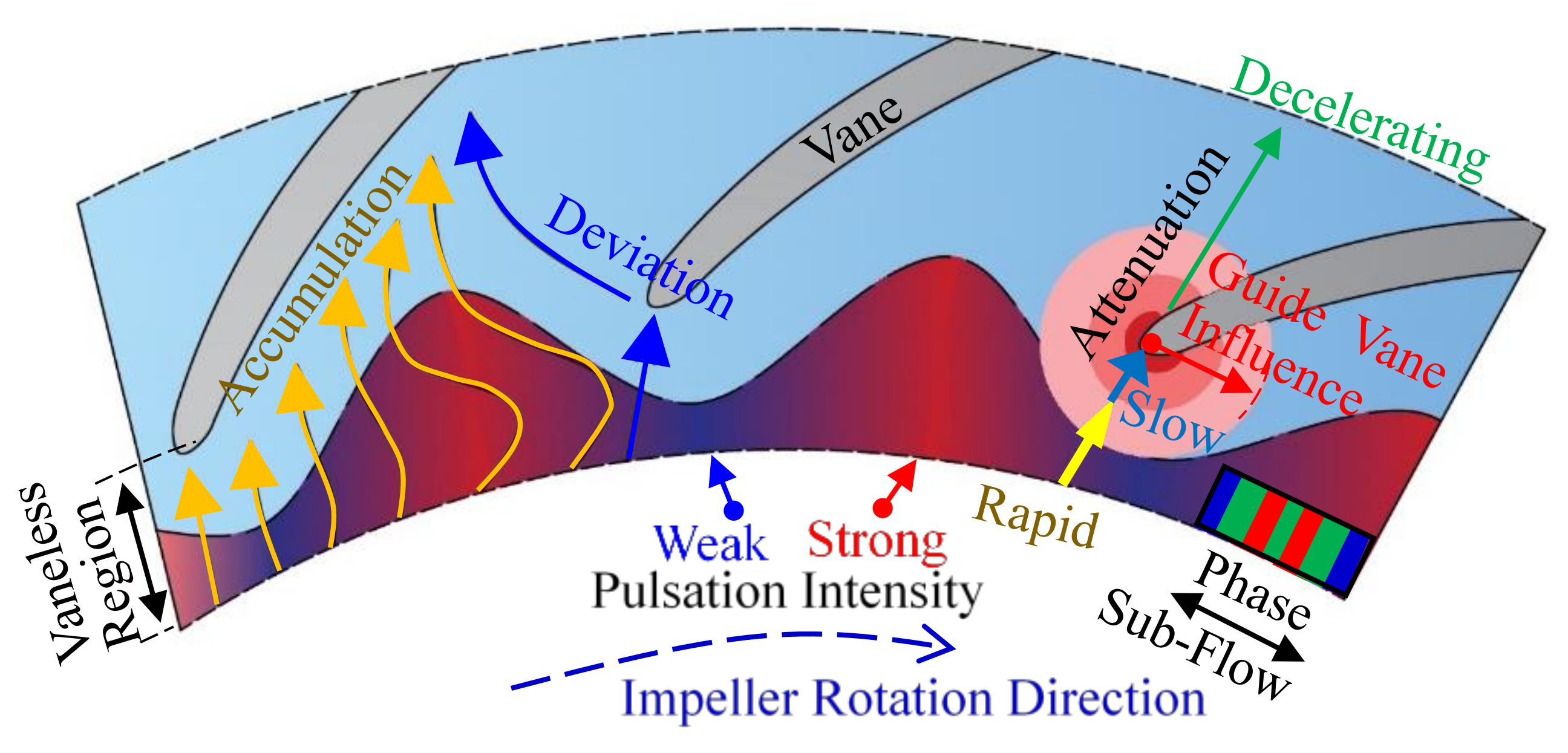
PTN results reveal the propagation and attenuation law of pressure pulsation frequencies in diffusers of the vaned-voluted pump. In the vaneless region, the pressure wave propagates along the radial direction. Vaned diffuser blades (and volute cut-water) have influence on the pressure pulsation. The accumulation effect and the flow-prevention effect of the vaned diffuser will cause local enhancement of amplitude. Hence, the pulsation amplitude attenuation has mainly three stages. In the vaneless region, it is rapid. Near the vaned diffuser, it attenuates first slowly then fast. After the vaned diffuser, the attenuation decelerates.
(4)
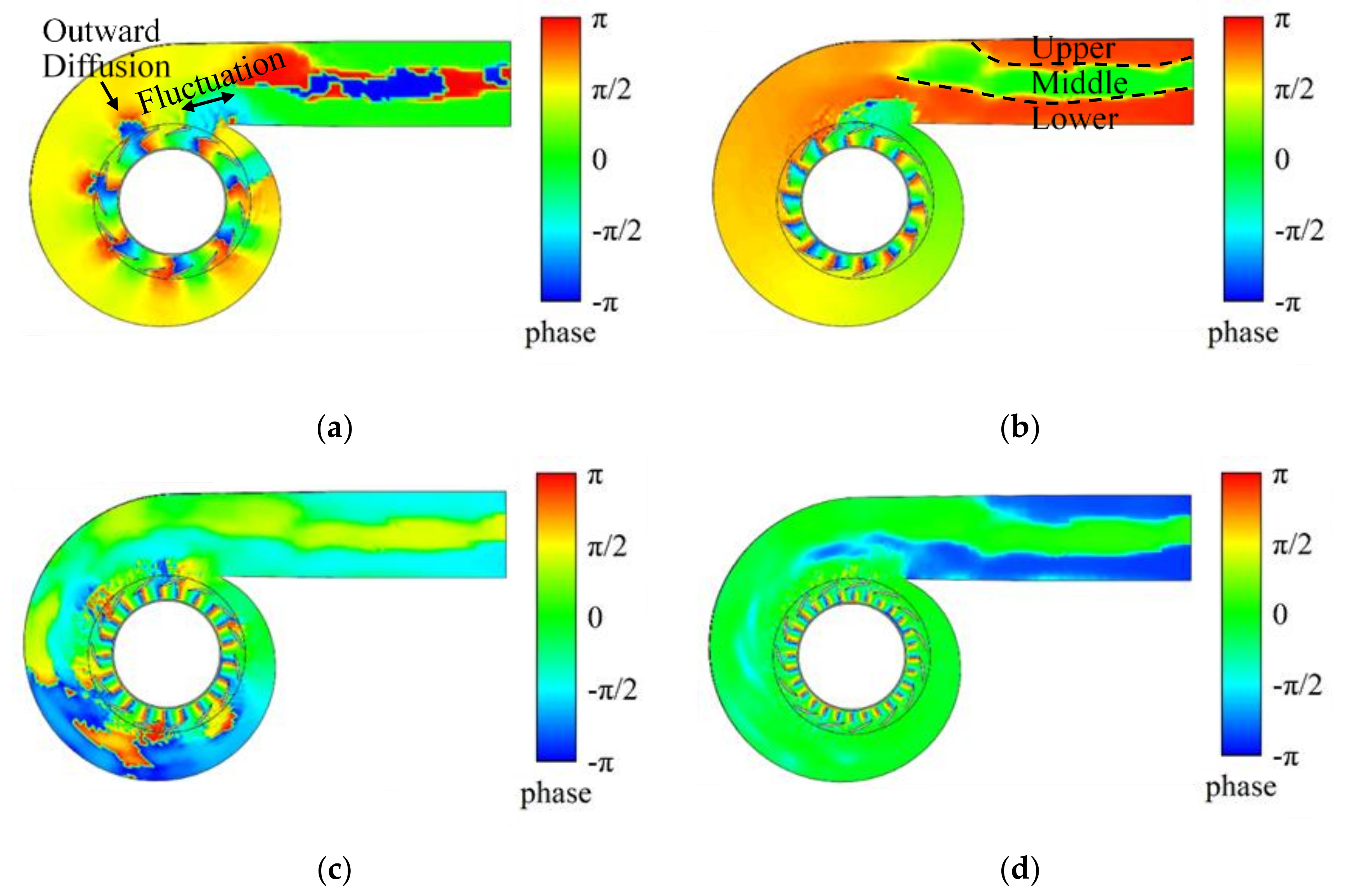
The phase distribution can indicate sub-flow with certain frequencies. BPF and BPF’s harmonics fluctuate from π to 0 to −π in the vaneless region along the circumferential direction. It shows the circumferential sub-flow driven by the impeller rotation. The outward diffusing pattern of BPF in the volute spiral section shows the sub-flow along the vaned diffuser in the streamwise direction. The fluctuating phase pattern between −0.5π and −π indicates local interference by several sub-flows, with some similar specific pulsation frequencies.
(5)
This study only analyzes the BPF and its harmonics at design condition. Considering the simplicity of the operation, the FFT method is selected. It has certain limitations. More reasonable distribution of the PTN points need to be studied, and better frequency domain analysis methods can be used so that more working conditions can be analyzed. The selection of the interpolation method also needs to be improved. This study can be combined with some typical physical phenomena, and further research will be developed in the future.

Author Contributions

Conceptualization, R.T., F.J. and Z.L.; methodology, Z.L.; software, Z.L.; validation, W.L., P.L. and Z.L.; formal analysis, Z.L.; resources, R.X.; data curation, F.J.; writing—original draft preparation, Z.L.; writing—review and editing, P.L.; visualization, F.J.; supervision, R.T.; project administration, R.T.; funding acquisition, R.T. and R.X. All authors have read and agreed to the published version of the manuscript.

Funding

This research was funded by National Natural Science Foundation of China, grant number No. 51909131 and National Natural Science Foundation of China, grant number No. 51879265.

Data Availability Statement

Data sharing not applicable.

Acknowledgments

The authors would like to acknowledge the financial support of National Natural Science Foundation of China No. 51909131 and National Natural Science Foundation of China No. 51879265.

Conflicts of Interest

The authors declare no conflict of interest.

Nomenclature

a 1 constant coefficient
A p pressure pulsation dimensionless coefficient
c n amplitude component
C 0 a constant term which represents a deviation from zero
C p the dimensionless coefficient of pressure
C R the dimensionless radius
D h the inlet diameter at hub, mm
D o u t impeller outlet diameter, mm
E total uncertainty
E r random uncertainty
E s systematic uncertainty
f frequency of pressure pulsation, Hz
f i the value at the sample point Pi
f s a p sampling frequency, Hz
F 1 blending function
F 2 second auxiliary function
g ( a ) the result of interpolation at the point A to be interpolated
GCI fine 21 convergence index of the grid of fine mesh and medium mesh
GCI fine 32 convergence index of the grid of medium mesh and coarse mesh
H head, m
H d design head, m
k kinetic energy
L s t Normalized Streamwise
M 1 First mesh scheme, fine mesh
M 2 Second mesh scheme, medium mesh
M 3 Third mesh scheme, coarse mesh
n d design rotational speed, r/min
n q specific speed
p pressure, Pa
p reference pressure at inflow inlet, Pa
Δ p the difference between instantaneous and average pressure value, Pa
p max the maximum pressure on this certain point, Pa
p min the minimum pressure on this certain point, Pa
P observation accuracy order
P e q v relative intensity of pressure pulsation
P i sample point for interpolation
P k production term of turbulent kinetic energy
P ω generating term of specific dissipation rate
Q flow rate, m3/s
Q d design flow rate, m3/s
R i o u t impeller outlet radius, mm
s invariant measure of the strain rate
s ( a ) the area of the A polygon
s i the area of the polygon near the point A
t time, s
t a c q total acquisition time, s
u ¯ i verage velocity, m/s
u i fluctuating velocity, m/s
w i ( a ) the weight of the interpolation point A
x i spatial coordinate, m
XYZlocal coordinate system
X T t The Fourier series (cosine signal form) of trigonometric function form
Z i m p impeller blade number
Z g vaned diffuser blade number
β constants of the turbulence model
β * constants of the turbulence model
e e x t 21 relative error of extrapolated value of fine mesh and medium mesh
e e x t 32 relative error of extrapolated value of medium mesh and coarse mesh
ϕ 1 evaluated variables of fine mesh
ϕ 2 evaluated variables of medium mesh
ϕ 3 evaluated variables of coarse mesh
ϕ e x t 21 extrapolated values of fine mesh and medium mesh
ϕ e x t 32 extrapolated values of medium mesh and coarse mesh
η efficiency
φ the dimensionless flow rate coefficient
φ d the design dimensionless flow rate coefficient
φ n initial phase angle of each sinusoidal function
μ dynamic viscosity, Pa·s
μ t turbulent eddy viscosity
θ circumferential angle, °
ρ density, kg/m3
σ k constants of the turbulence model
σ ω constants of the turbulence model
ω specific dissipation rate
ω r rotation angular speed of impeller, rad/s
ω f angular frequency
ψ the dimensionless head coefficient
ψ d the design dimensionless head coefficient
BPFBlade Passing Frequency
CFDcomputational fluid dynamics
FFTfast Fourier transform
PTNpulsation tracking network
RANSReynolds averaged Navier Stokes
URANSunsteady Reynolds averaged Navier Stokes

References

  1. McKee, K.K.; Forbes, G.; Mazhar, I.; Entwistle, R.; Howard, I. A review of major centrifugal pump failure modes with application to the water supply and sewerage industries. In Proceedings of the ICOMS Asset Management Conference, Gold Coast, Australia, 16–20 May 2011. [Google Scholar]
  2. Pei, J.; Yuan, S.; Li, X.; Yuan, J. Numerical prediction of 3-d periodic flow unsteadiness in a centrifugal pump under part load condition. J. Hydrodyn. B 2014, 26, 257–263. [Google Scholar] [CrossRef]
  3. Tao, R.; Xiao, R.; Liu, W. Investigation of the flow characteristics in a main nuclear power plant pump with eccentric impeller. Nucl. Eng. Design 2018, 327, 70–81. [Google Scholar] [CrossRef]
  4. Yao, Z.; Wang, F.; Qu, L.; Xiao, R.; He, C.; Wang, M. Experimental investigation of time-frequency characteristics of pressure fluctuations in a double-suction centrifugal pump. J. Fluids Eng. 2011, 133, 1076–1081. [Google Scholar] [CrossRef]
  5. Wei, Z.; Yang, W.; Xiao, R. Pressure fluctuation and flow characteristics in a two-stage double-suction centrifugal pump. Symmetry 2019, 11, 65. [Google Scholar] [CrossRef] [Green Version]
  6. Guelich, J.F.; Bolleter, U. Pressure pulsations in centrifugal pumps. J. Vib. Acoust. 1992, 114, 272–279. [Google Scholar] [CrossRef]
  7. Dong, R.; Chu, S.; Katz, J. Effect of modification to tongue and impeller geometry on unsteady flow, pressure fluctuations, and noise in a centrifugal pump. J. Turbomach. 1997, 119, 506–515. [Google Scholar] [CrossRef] [Green Version]
  8. Morgenroth, M.; Weaver, D.S. Sound generation by a centrifugal pump at blade passing frequency. J. Turbomach. 1998, 120, 736–743. [Google Scholar] [CrossRef]
  9. Song, H.; Zhang, J.; Huang, P.; Cai, H.; Cao, P.; Hu, B. Analysis of Rotor-Stator Interaction of a Pump-Turbine with Splitter Blades in a Pump Mode. Mathematics 2020, 8, 1465. [Google Scholar] [CrossRef]
  10. Zhang, Y.; Zheng, X.; Li, J.; Du, X. Experimental study on the vibrational performance and its physical origins of a prototype reversible pump turbine in the pumped hydro energy storage power station. Renew. Energy 2019, 130, 667–676. [Google Scholar] [CrossRef]
  11. Ran, H.; Luo, X.; Zhu, L.; Zhang, Y. Experimental study of the pressure fluctuations in a pump turbine at large partial flow conditions. Chin. J. Mech. Eng. 2012, 25, 1205–1209. [Google Scholar] [CrossRef]
  12. Zhang, N.; Gao, B.; Ni, D.; Liu, X. Coherence analysis to detect unsteady rotating stall phenomenon based on pressure pulsation signals of a centrifugal pump. Mech. Syst. Signal 2021, 148, 107161. [Google Scholar] [CrossRef]
  13. Sinha, M.; Pinarbasi, A.; Katz, J. The flow structure during onset and developed states of rotating stall within a vaned diffuser of a centrifugal pump. J. Fluids Eng. 2001, 123, 490–499. [Google Scholar] [CrossRef] [Green Version]
  14. González, J.; Fernández, J.; Blanco, E.; Santolaria, C. Numerical simulation of the dynamic effects due to impeller-volute interaction in a centrifugal pump. J. Fluids Eng. 2002, 124, 348–355. [Google Scholar] [CrossRef]
  15. Parrondo-Gayo, J.L.; González-Pérez, J.; Fernández-Francos, J. The effect of the operating point on the pressure fluctuations at the blade passage frequency in the volute of a centrifugal pump. J. Fluids Eng. 2002, 124, 784–790. [Google Scholar] [CrossRef]
  16. Zhang, N.; Yang, M.; Gao, B.; Li, Z.; Ni, D. Investigation of rotor-stator interaction and flow unsteadiness in a low specific speed centrifugal pump. Stroj. Vestn.-J. Mech. Eng. 2016, 62, 21–31. [Google Scholar] [CrossRef]
  17. Wang, H.; Tsukamoto, H. Experimental and numerical study of unsteady flow in a diffuser pump at off-design conditions. J. Fluids Eng. 2003, 125, 767–778. [Google Scholar] [CrossRef]
  18. Lei, T.; Zhu, B.; Cao, S.; Wang, Y.; Wang, B. Numerical simulation of unsteady cavitation flow in a centrifugal pump at off-design conditions. Proc. Inst. Mech. Eng. Part C J. Mech. Eng. Sci. 2014, 228, 1994–2006. [Google Scholar] [CrossRef]
  19. Lei, T.; Zhu, B.; Wang, Y.; Cao, S.; Gui, S. Numerical study on characteristics of unsteady flow in a centrifugal pump volute at partial load condition. Eng. Comput. 2015, 32, 1549–1566. [Google Scholar]
  20. Wang, F.; Zhang, L.; Zhang, Z. Analysis on pressure fluctuation of unsteady flow in axial-flow pump. J. Hydraul. Eng. 2007, 38, 1003–1009. [Google Scholar]
  21. Zhang, D.; Shi, W.; Chen, B.; Guan, X. Unsteady flow analysis and experimental investigation of axial-flow pump. J. Hydrodyn. B 2010, 22, 35–43. [Google Scholar] [CrossRef]
  22. Wang, C.; Wang, F.; Tang, Y.; Wang, B.; Yao, Z.; Xiao, R. Investigation on the horn-like vortices in stator corner separation flow in an axial flow pump. J. Fluids Eng. 2020, 142, 071208. [Google Scholar] [CrossRef]
  23. Jin, F.; Yao, Z.; Li, D.; Xiao, R.; Wang, F.; He, C. Experimental investigation of transient characteristics of a double suction centrifugal pump system during starting period. Energies 2019, 12, 4135. [Google Scholar] [CrossRef] [Green Version]
  24. Spence, R.; Amaral-Teixeira, J. A CFD parametric study of geometrical variations on the pressure pulsations and performance characteristics of a centrifugal pump. Comput. Fluids 2009, 38, 1243–1257. [Google Scholar] [CrossRef] [Green Version]
  25. Zeng, Y.; Yao, Z.; Wang, F.; Xiao, R.; He, C. Experimental investigation on pressure fluctuation reduction in a double suction centrifugal pump: Influence of impeller stagger and blade geometry. J. Fluids Eng. 2020, 142, 041202. [Google Scholar] [CrossRef]
  26. Sun, Y.; Zuo, Z.; Liu, S.; Liu, J.; Wu, Y. Numerical study of pressure fluctuations in different vaned diffusers’ opening angle in pump mode of a pump turbine. In Proceedings of the 26th IAHR Symposium on Hydraulic Machinery and Systems, Beijing, China, 19–23 August 2012. [Google Scholar]
  27. Sun, Y.; Zuo, Z.; Liu, S.; Liu, J.; Wu, Y. Distribution of pressure fluctuations in a prototype pump turbine at pump model. Adv. Mech. Eng. 2014, 2014, 174–183. [Google Scholar]
  28. Zhu, D.; Xiao, R.; Tao, R.; Liu, W. Analysis of flow regime and pressure pulsations under off-design condition in pump mode of pump-turbine. Trans. Chin. Soc. Agric. Mach. 2016, 47, 77–84. (In Chinese) [Google Scholar]
  29. Farzaneh-Gord, M.; Faramarzi, M.; Ahmadi, M.H.; Sadi, M.; Shamshirband, S.; Mosavi, A.; Chau, K. Numerical simulation of pressure pulsation effects of a snubber in a CNG station for increasing measurement accuracy. Eng. Appl. Comput. Fluid Mech. 2019, 13, 642–663. [Google Scholar] [CrossRef] [Green Version]
  30. Lai, B.; Cui, Q.; Han, L.; Gong, R.; Wang, Q. Pressure fluctuation of 1000 mw model francis turbine. Large Electr. Mach. Hydraul. Turbine 2018, 258, 47–52. [Google Scholar]
  31. Wu, C.; Zhang, W.; Wu, P.; Yi, J.; Ye, H.; Huang, B.; Wu, D. Effects of blade pressure side modification on unsteady pressure pulsation and flow structures in a centrifugal pump. J. Fluids Eng. 2021, 143, 111208. [Google Scholar] [CrossRef]
  32. Lin, Y.; Li, X.; Li, B.; Jia, X.; Zhu, Z. Influence of impeller sinusoidal tubercle trailing edge on pressure pulsation in a centrifugal pump at nominal flow rate. J. Fluids Eng. 2021, 143, 091205. [Google Scholar] [CrossRef]
  33. Posa, A. LES investigation on the dependence of the flow through a centrifugal pump on the diffuser geometry. Int. J. Heat Fluid Flow 2021, 87, 108750. [Google Scholar] [CrossRef]
  34. Wang, F.; Yao, Z.; Wei, Y.; Xiao, R.; Leng, H. Impeller design with alternate loading technique for double-suction centrifugal pumps. Trans. Chin. Soc. Agric. Mach. 2015, 46, 84–91. (In Chinese) [Google Scholar]
  35. Zeng, Y.; Yao, Z.; Tao, R.; Liu, W.; Xiao, R. Effects of lean mode of blade trailing edge on pressure fluctuation characteristics of a vertical centrifugal pump with vaned diffuser. J. Fluids Eng. 2021, 143, 111201. [Google Scholar] [CrossRef]
  36. Tanasa, C.; Bosioc, A.; Muntean, S.; Susan-Resiga, R. Flow-feedback control technique for vortex rope mitigation from conical diffuser of hydraulic turbines. Proc. Rom. Acad. Ser. A 2011, 12, 125–132. [Google Scholar]
  37. Tanasa, C.; Szakal, R.; Mos, D.; Ciocan, T.; Muntean, S. Experimental and numerical analysis of decelerated swirling flow from the discharge cone of hydraulic turbines using pulsating jet technique. IOP Conf. Ser. Earth Environ. Sci. 2019, 240, 022010. [Google Scholar] [CrossRef]
  38. Tanasa, C.; Bosioc, A.; Muntean, S.; Susan-Resiga, R. A novel passive method to control the swirling flow with vortex rope from the conical diffuser of hydraulic turbines with fixed blades. Appl. Sci. 2019, 22, 4910. [Google Scholar] [CrossRef] [Green Version]
  39. Bosioc, A.; Susan-Resiga, R.; Muntean, S.; Tanasa, C. Unsteady pressure analysis of a swirling flow with vortex rope and axial water injection in a discharge cone. J. Fluids Eng. 2012, 134, 669–679. [Google Scholar] [CrossRef]
  40. International Electrotechnical Commission. Hydraulic Turbines, Storage Pumps and Pump-Turbines-Model Acceptance Tests, 2nd ed.; International Standard IEC 60193; International Electrotechnical Commission: Lausanne, Switzerland, 1999. [Google Scholar]
  41. Launder, B.E.; Spalding, D.B. Lectures in Mathematical Models of Turbulence, 1st ed.; Academic Press: London, UK, 1972. [Google Scholar]
  42. Yakhot, V.; Orzag, S.A. Renormalization group analysis of turbulence: Basic theory. J. Sci. Comput. 1986, 1, 3–11. [Google Scholar] [CrossRef]
  43. Shih, T.H.; Liou, W.W.; Shabbir, A.; Yang, Z.; Zhu, J. A new k-ε eddy viscosity model for high Reynolds number turbulent flows. Comput. Fluids 1995, 24, 227–238. [Google Scholar] [CrossRef]
  44. Wilcox, D.C. Multiscale model for turbulent flows. AIAA J. 1986, 26, 1311–1320. [Google Scholar] [CrossRef]
  45. Menter, F.R. Two-equation eddy-viscosity turbulence models for engineering applications. AIAA J. 1994, 32, 1598–1605. [Google Scholar] [CrossRef] [Green Version]
  46. Wang, Y.; Liu, H.; Yuan, S.; Tan, M.; Shu, M. Applicability of turbulence models on characteristics prediction of centrifugal pumps. In Proceedings of the ASME-JSME-KSME Joint Fluids Engineering Conference, Hamamatsu, Japan, 24–29 July 2011. [Google Scholar]
  47. Liu, H.; Pan, H. The influence of turbulence model selection and leakage considerations on CFD simulation results for a centrifugal pump. In Proceedings of the Global Conference on Civil, Structural and Environmental Engineering/3rd International Symp on Multi-field Coupling Theory of Rock and Soil Media and its Applications, Yichang, China, 20–21 October 2012. [Google Scholar]
  48. Al-Obaidi, A.R. Effects of Different Turbulence Models on Three-Dimensional Unsteady Cavitating Flows in the Centrifugal Pump and Performance Prediction. Int. J. Nonlinear Sci. Num. Simul. 2019, 20, 487–509. [Google Scholar] [CrossRef]
  49. Brigham, E.O. The Fast Fourier Transform.; Prentice Hall: Englewood Cliffs, NJ, USA, 1974. [Google Scholar]
  50. Sibson, R. A brief description of natural neighbor interpolation. In Interpreting Multivariate Data; Barnett, V., Ed.; John Wiley: Chichester, UK, 1981; pp. 21–36. [Google Scholar]
  51. Celik, I.B.; Ghia, U.; Roache, P.J.; Freitas, C.J. Procedure for Estimation and Reporting of Uncertainty Due to Discretization in CFD Applications. J. Fluids Eng. 2008, 130, 078001. [Google Scholar]
Figure 1. Structures of the large-scale vaned-voluted centrifugal pump model.
Machines 09 00266 g001
Figure 2. Schematic map of the test rig.
Machines 09 00266 g002
Figure 3. Pressure-pulsation monitor points in the model, test, and numerical simulation.
Machines 09 00266 g003
Figure 4. Schematic map of the natural neighbor interpolation method.
Machines 09 00266 g004
Figure 5. Distribution of PTN in the vaneless region, the vaned diffuser, and the volute on Z = 0 plane.
Machines 09 00266 g005
Figure 6. Flow domain of the pump model.
Machines 09 00266 g006
Figure 7. Four monitors points of GCI.
Machines 09 00266 g007
Figure 8. Mesh of the computational domain of the pump unit.
Machines 09 00266 g008
Figure 9. Comparison between CFD and experimental dimensionless head ψ and efficiency η.
Machines 09 00266 g009
Figure 10. Comparison between CFD and experimental pressure pulsation at φ d . (a) VS + X; (b) VS − X; (c) VS + Y; (d) VS − Y.
Machines 09 00266 g010aMachines 09 00266 g010b
Figure 11. Flow pattern overview in the pump at φ d on Z = 0 plane and impeller mid-span surface. (a) Indication of Z = 0 plane and impeller mid-span surface; (b) pressure contour and velocity vectors.
Machines 09 00266 g011aMachines 09 00266 g011b
Figure 12. Comparison between CFD and experimental pressure pulsation at φ d . (a) Pa1; (b) Pa2; (c) Pa3; (d) Pa4.
Machines 09 00266 g012aMachines 09 00266 g012b
Figure 13. Main frequency distribution on Z = 0 plane.
Machines 09 00266 g013
Figure 14. Ap amplitude contour of typical frequencies on the Z = 0 plane. (a) 140 Hz; (b) 280 Hz; (c) 420 Hz; (d) 560 Hz.
Machines 09 00266 g014aMachines 09 00266 g014b
Figure 15. P e q v amplitude contour of typical frequencies on Z = 0 plane. (a) 140 Hz; (b) 280 Hz; (c) 420 Hz; (d) 560 Hz.
Machines 09 00266 g015
Figure 16. Reference angle and positions for analyzing the detailed distribution of amplitude on the Z = 0 plane.
Machines 09 00266 g016
Figure 17. Circumferential amplitude of A p and P e q v distribution. (a) 140 Hz; (b) 280 Hz.
Machines 09 00266 g017
Figure 18. Radial amplitude of A p distribution. (a) 140 Hz; (b) 280 Hz; ① impeller blade trailing-edge downstream region; ② amplitude fluctuation region; ③ vaneless attenuation region; ④ pre-guide-vane fluctuating region; ⑤ inter-channel attenuation region; ⑥ post-guide-vane attenuation.
Machines 09 00266 g018
Figure 19. Streamwise lines amplitude of A p .
Machines 09 00266 g019
Figure 20. Phase difference distribution on Z = 0 plane. (a) 140 Hz; (b) 280 Hz; (c) 420 Hz; (d) 560 Hz.
Machines 09 00266 g020
Figure 21. Illustrations for discussion. RSI: rotor-stator interface.
Machines 09 00266 g021
Table 1. Main parameters and values of the pump unit.
ParameterAbbreviationValue
Design flow rate Q d 0.273 [m3/s]
Design head H d 22 [m]
Design rotational speed n d 1200 [r/min]
Impeller blade number Z i m p 7
Vaned diffuser blade number Z g 15
Impeller outlet diameter D o u t 392 [mm]
The inlet diameter at hub D h 280 [mm]
Specific speed n q 61.72
Table 2. Test instruments and uncertainty.
QuantityApparatusTypeUncertainty
Flow rateElectromagnetic flowmeterKrohne IFC090±0.18%
Rotation speedRotary encoderE6B2-CWZ1X±0.02%
HeadDifferential pressure sensorRosemount 3051±0.05%
TorqueLoad sensorHBM Z3H2R±0.05%
Pressure pulsationDynamic pressure sensorPCB 112A22±1.00%
Table 3. Evaluation results of discretization error.
VariationVS + XZ=0VS − XZ=0VS + YZ=0VS − YZ=0ηH
ϕ 1 −20,434−28,013−19,088−25,07689.60%21.0574
ϕ 2 −19,253−27,842−18,338−24,58989.67%21.0886
ϕ 3 −16,647−25,171−16,553−21,07490.37%21.009
P2.1778.4013.40031.62624.71551.9896
ϕ ext 21 −21,793−28,030−19,835−25,18389.59%21.0344
e ext 21 6.2%0.06%3.76%0.42%0.012%0.1092%
GCI fine 21 8.3%0.07%4.89%0.53%0.015%0.1364%
ϕ ext 32 −21,793−28,030−19,835−25,18389.59%21.1373
e ext 32 11.6%0.67%7.55%2.36%0.09%0.2305%
GCI fine 32 16%0.84%10.20%3.02%0.11%0.2889%
Table 4. Mesh number details of the computational domain.
PartElement TypeNodesElements
InletHexahedral203307196776
ImpellerHexahedral11344201029924
Vaned diffuserHexahedral17193601581300
Volute Hexahedral688800665556
Total-37458873473556
Publisher’s Note: MDPI stays neutral with regard to jurisdictional claims in published maps and institutional affiliations.

