Optimal PID Controllers for AVR System Considering Excitation Voltage Limitations Using Hybrid Equilibrium Optimizer

Abstract

Automatic voltage regulator (AVR) represents the basic voltage regulator loop in power systems. The central part of this loop is the regulator, which has parameters that define the speed of the voltage regulation, quality of responses, and system stability. Furthermore, it has an impact on the excitation voltage change and value, especially during transients. In this paper, unlike literature approaches, the experimental verifications of the impact of regulator parameters on the excitation voltage and current value are presented. A novel hybrid metaheuristic algorithm for obtaining regulator parameters determination of the AVR system, and a novel regulator design taking into account excitation voltage limitation are presented. The proposed algorithm combines the properties and characteristics of equilibrium optimizer and evaporation rate water cycle algorithms. The proposed algorithm is effective, fast, and accurate. Both experimental and simulation results show that the limitation of the excitation voltage increases the settling time of the generator voltage during reference change. Additionally, the simulation results show that the optimal values of PID parameters are smaller for limited excitation voltage values.

1. Introduction

Power systems are dynamic in nature, where their operators must monitor all consumers, and regulate energy production of the various energy sources operating and stored. Furthermore, at any moment, the quality of energy, in terms of voltage level and frequency, needs to be in predefined limits [1]. Automatic voltage regulation is an essential control loop for the generator voltage regulation on the desired value [1,2,3]. By regulating the generator voltage, the voltage in power systems can be efficiently controlled. However, that process depends on the excitation system readiness, and the speed of regulation relies on the regulator parameters. In a mathematical sense, all components of the excitation systems are nonlinear which indicates that the observation of an automatic regulation loop is not an easy task, particularly with certain assumptions that should be considered [4].

The most important part of the automatic voltage regulator (AVR) is the regulator. Although different variants of regulators can be found in science and practice, the most common regulator is still the proportional-integral-derivative (PID) regulator. Furthermore, different types of PID regulators can be found in the literature—ideal PID [4,5,6,7,8,9,10,11,12,13,14,15,16,17], real PID [18,19,20,21], fractional-order PID (FOPID) [17,22,23,24,25,26,27,28,29,30], as well as the higher-order controllers, such as PIDD² [17,31].

In practice, the majority of tuning methods are based on a process model or on some non-parametric data from the process. In terms of the controller tuning based on optimal point search, the research works [4,5,6,7,8,9,10,11,12,13,14,15,16,17,18,19,20,21,22,23,24,25,26,27,28,29,30,31] use different algorithms to design the controller of the AVR system. Some of these works present the usage of improved kidney-inspired algorithm (IKIA) [4], whale optimization algorithm (WOA) [5], symbiotic organisms search algorithm (SOSA) [6], ant colony optimization (ACO) [8], local unimodal sampling algorithm (LUSA) [9], taguchi combined genetic algorithm (TCGA) [10], simplified particle swarm optimization (SPSO) [11], genetic algorithm (GA) [12], artificial bee colony algorithm (ABCA) [13], chaotic optimization approach (COA) [14], particle swarm optimization (PSO) [15], equilibrium optimizer algorithm (EOA) [16], hybrid simulated annealing- manta ray foraging optimization algorithm (SA-MRFA) [17], cuckoo search algorithm (CSA) [19,27], teaching-learning based optimization (TLBO) [20], chaotic multi-objective optimization (CMOA) [22,25], artificial bee colony algorithm (ABCA) [23], chaotic ant swarm (CAS) [24], multi-objective extremal optimization (MOEO) [26], salp swarm optimization (SSO) [29], and yellow saddle goatfish algorithm (YSGA) [30] for this purpose.

All the previously mentioned algorithms use different objective functions. The most commonly used objective function takes into account different time-domain parameters [22,23,24,25,26,27,28,29], such as rise time, settling time, overshoot, and steady state error. However, there are other objective functions in the literature which rely on different frequency-domain parameters [22] such as gain margin, phase margin, gain crossover frequency, and others. In this regard, the most common objective functions are the integrated absolute error (IAE) and integral time absolute error (ITAE) as mentioned in [23,26,29]. Moreover, Zwee Lee Gaing’s function is another common objective function [24,27] that takes into account different time-domain parameters. It is apparent that investigation of the performance of different optimization algorithms, as well as the objective functions, is popular in solving this engineering problem.

In this paper, a novel hybrid metaheuristic algorithm, called equilibrium optimizer–evaporation rate water cycle algorithm (EO–ERWCA) is presented and tested. The mentioned hybrid algorithm belongs to the hybrid algorithms that rely on sub-populations. The main idea of the hybridization of this algorithm is to split the population into two sub-populations, and then separately apply the first EO algorithm to one sub-population and the second ER-WCA algorithm to the other.

Although many research works are dealing with PID parameters design for AVR control, all of them have two significant drawbacks. Firstly, the experimental results of the impact of different PID parameters on excitation voltage, excitation current, and generator voltage have not been presented in these works. Accordingly, in this paper, experimental validation of the controller performance is presented and analyzed. Secondly, the research works did not take into account the excitation voltage limit. Namely, field winding determines the rated value of the excitation voltage as well as its allowable value during transients. Furthermore, the field voltage determines the field current and its unlimited value can damage the field coils. Therefore, in practice, the field voltage cannot be unlimited. In practice, the maximum excitation voltage during the “forcing” of the excitation current (known as ceiling voltage) is in the range between 1.6 p.u (p.u denotes a per-unit value) and 3 p.u [3,32,33]. The ceiling voltages above 2 p.u are difficult to realize because of magnetic saturation [3]. Additionally, in this case, the field current is impossible to be observed and controlled. Therefore, in a real power system, an excitation voltage value higher than 3 p.u cannot be realized. This problem is noted in [32,33]. In [32], the excitation voltage is limited by limiters, which can be represented by upper and lower limits. The limiters represent the elements for the limitation of the amplitude and speed of change of certain variables. In the excitation system, the limits are set only for variables that have a significant impact on the minimum and maximum excitation voltage or current value. Typically, in excitation systems, there are two types of limiters—windup and anti-windup. Windup protection is based on setting the output variable (excitation voltage) to the corresponding minimum/maximum limit value if it exceeds the pre-defined limits. On the other side, the anti-windup protection, despite considering the value of the output variable, also takes into account its speed of change. In other words, the anti-windup changes the states of the controller when there is a difference between unlimited and limited controller output. A block diagram of the AVR structure with the limiter is presented in [32]. However, taking into account that the excitation voltage limit is not concerned in previously published papers dealing with the AVR controller design.

In [33], the excitation voltage limit was taken into account during PID parameters design. Furthermore, several comparisons among different PID values in terms of the excitation voltage value were introduced. However, in both papers, experimental validation of the controller performance was not presented. Additionally, the impact of excitation voltage/current limitation on the optimal PID parameters design was not analyzed. These issues represent the research goal of this work.

The organization of this paper is as follows. Section 2 gives a short overview of the composition of the AVR system. A comparison of the literature approaches that deal with the optimization of different types of PID controllers, with excitation voltage discussion, is given in Section 3. A detailed description and mathematical formulation of the proposed EO–ERWCA algorithm are given in Section 4. Section 5 shows the results obtained from the simulations that are carried out in this paper. The experimental investigation of the impact of the excitation voltage and AVR controller values on the generator voltage response is presented in Section 6. Finally, conclusions are presented in Section 7.

2. Automatic Voltage Regulation System

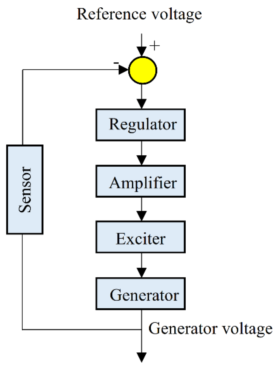
The AVR system consists of five components—regulator (R), amplifier (A), exciter (E), generator (G), and sensor (S). The block diagram of an AVR system is illustrated in Figure 1. The regulator uses the signal obtained from the difference between the reference and measured (sensed) generator voltage and generates a control signal for the amplifier to amplify the signal. In modern excitation systems, it is a microprocessor unit. The most-used regulator in AVR systems is the PID regulator. The ideal PID regulator is not often used [4,5,6,7,8,9,10,11,12,13,14,15,16,17] in the literature. Some research works present the usage of real PID (in which the derivative action is filtered) [18,19,20,21], fractional-order PID regulator (in which the fractional calculus is added to the PID regulator) [22,23,24,25,26,27,28,29,30], and higher-order controller or PIDD² [31].

The ideal PID regulator has three parameters i.e., gains—proportional k_p, integral k_i, and differential k_d. The transfer function of the ideal PID regulator in the s-domain is given as follows:

$$PI{D}_{ideal}\left(s\right)=k_p+\frac{k_i}{s}+k_{d}s$$

(1)

In a real PID controller, the derivative action of the ideal PID controller is filtered with the filter time constant T_f. Its transfer function is given as follows:

$$PI{D}_{real}=k_p+\frac{k_i}{s}+k_d\left(\frac{s}{1+T_{f}s}\right)$$

(2)

The FOPID controller has five parameters k_p, k_i, k_d, μ, and λ, where μ and λ represent the order of the derivative and the integral. The FOPID transfer function is given as follows:

$$FOPID=k_p+\frac{k_i}{s^{\lambda }}+k_d{s}^{\mu }$$

(3)

The PIDD² controller has also an additional parameter that represents second-order derivative gain (k_d2), in addition to the standard parameters k_p, k_i, and k_d. Its transfer function is given as follows:

$$PID{D}^2=k_p+\frac{k_i}{s}+k_{d}s+k_{d2}{s}^2$$

(4)

The amplifier is a power element, which increases the power of the control signal and generates a signal of appropriate power for the exciter control. Mathematically, the amplifier can be represented as a first-order transfer function W_A with gain k_A and time constant T_A as follows:

$$W_A\left(s\right)=\frac{k_A}{1+s{T}_A}$$

(5)

In modern power systems, the exciter represents the power electronic device, usually, it is a thyristor rectifier bridge. This device receives the control signal from the amplifier and defines the excitation voltage value. At present, power electronic devices, such as rectifier bridges, are fast and easy to be controlled. They can be mathematically represented as a first-order transfer function W_E with gain k_E and time constant T_E as follows:

$$W_E\left(s\right)=\frac{k_E}{1+s{T}_E}$$

(6)

The most complicated element in the excitation system is the synchronous machine. The most frequently used model of the synchronous generator (SG) is very complicated and it consists of seven differential equations, which are derived from Park’s transformations. However, in the literature, all the components of an AVR loop are formulated as first-order transfer functions W_G with gain k_G and time constant T_G as follows:

$$W_G\left(s\right)=\frac{k_G}{1+s{T}_G}$$

(7)

The parameters of generator, exciter, amplifier and sensor used are the same in all research—k_G = 1, T_G = 1, k_E = 1, T_E = 0.4, k_A = 10, T_A = 0.1.

3. Related Works

In this section, an overview of the existing studies dealing with PID design in AVR systems is presented.

Table 1. Summary of the optimal parameters obtained using different controllers/algorithms in the investigated works.

Method Number	Ref.	Regulator	kp	ki	kd	Tf	μ	λ	kd2
1	[4]	Ideal PID	1.0426	1.0093	0.5999	-	-	-	-
2	[5]		0.7847	0.9961	0.3061	-	-	-	-
3	[6]		0.5693	0.4097	0.1750	-	-	-	-
4	[7]		0.9685	1.0000	0.8983	-	-	-	-
5			0.9519	0.9997	0.8994	-	-	-	-
6			0.86832	0.9325	0.9419	-	-	-	-
7	[8]		0.6739	0.5951	0.2622	-	-	-	-
8			0.6348	0.4801	0.2267	-	-	-	-
9	[9]		1.2012	0.9096	0.4593	-	-	-	-
10			0.5878	0.4062	0.1843	-	-	-	-
11			0.6022	0.3793	0.1841	-	-	-	-
12			1.2930	0.9828	0.6303	-	-	-	-
13			0.6190	0.4222	0.2058	-	-	-	-
14	[10]		0.5600	0.5000	0.2000	-	-	-	-
15	[11]		0.5857	0.4189	0.1772	-	-	-	-
16			0.9931	0.7461	0.4249	-	-	-	-
17			0.9877	0.7780	0.5014	-	-	-	-
18			0.9544	0.9434	0.9909	-	-	-	-
19	[12]		0.6823	0.6138	0.2678	-	-	-	-
20			0.6800	0.5221	0.2440	-	-	-	-
21			0.6727	0.4786	0.2298	-	-	-	-
22	[13]		1.6524	0.4083	0.3654	-	-	-	-
23	[14]		0.6710	0.5050	0.2640	-	-	-	-
24			0.6390	0.4770	0.2340	-	-	-	-
25			0.6480	0.4780	0.2410	-	-	-	-
26			0.6220	0.4530	0.2180	-	-	-	-
27			0.6590	0.4870	0.2540	-	-	-	-
28	[15]		0.6568	0.5393	0.2458	-	-	-	-
29			0.6751	0.5980	0.2630	-	-	-	-
30			0.6570	0.5390	0.2458	-	-	-	-
31			0.6271	0.4652	0.2209	-	-	-	-
32			0.6477	0.5128	0.2375	-	-	-	-
33			0.6476	0.5216	0.2375	-	-	-	-
34	[16]		0.6829	0.6321	0.2716	-	-	-	-
35	[17]		0.6778	0.3802	0.2663	-	-	-	-
36	[18]	Real PID	0.6392	0.4757	0.2159	0.0021	-	-	-
37			0.3120	0.2567	0.1503	0.002	-	-	-
38			0.5463	0.3409	0.1485	0.002	-	-	-
39	[19]		0.6198	0.4165	0.2126	0.001	-	-	-
40	[20]		0.5302	0.4001	0.1787	0.0057	-	-	-
41	[21]		0.7080	0.6560	0.2820	0.001	-	-	-
42	[22]	FOPID	0.408	0.374	0.1773	-	1.3336	0.6827	-
43			0.9632	0.3599	0.2816	-	1.8307	0.5491	-
44			1.0376	0.3657	0.6546	-	1.8716	0.5497	-
45	[23]		1.9605	0.4922	0.2355	-	1.4331	1.5508	-
46	[24]		1.0537	0.4418	0.251	-	1.1122	1.0624	-
47			0.9315	0.4776	0.2536	-	1.0838	1.0275	-
48	[25]		0.9894	1.7628	0.3674	-	0.7051	0.9467	-
49			0.8399	1.3359	0.3511	-	0.7107	0.9146	-
50			0.4667	0.9519	0.2967	-	0.2306	0.8872	-
51	[26]		2.9737	0.9089	0.5383	-	1.3462	1.1446	-
52	[27]		2.5490	0.1759	0.3904	-	1.3800	0.9700	-
53			2.5150	0.1629	0.3888	-	1.3800	0.9700	-
54			2.4676	0.302	0.4230	-	1.3800	0.9700	-
55	[28]		1.5338	0.6523	0.9722	-	1.2090	0.9702	-
56	[29]		1.9982	1.1706	0.5749	-	1.1656	1.1395	-
57	[30]		1.7775	0.9463	0.3525	-	1.2606	1.1273	-
58	[17]		1.8931	0.8699	0.3595		1.2780	1.0408
59	[31]	PIDD2	2.7784	1.8521	0.9997	-	-	-	0.073
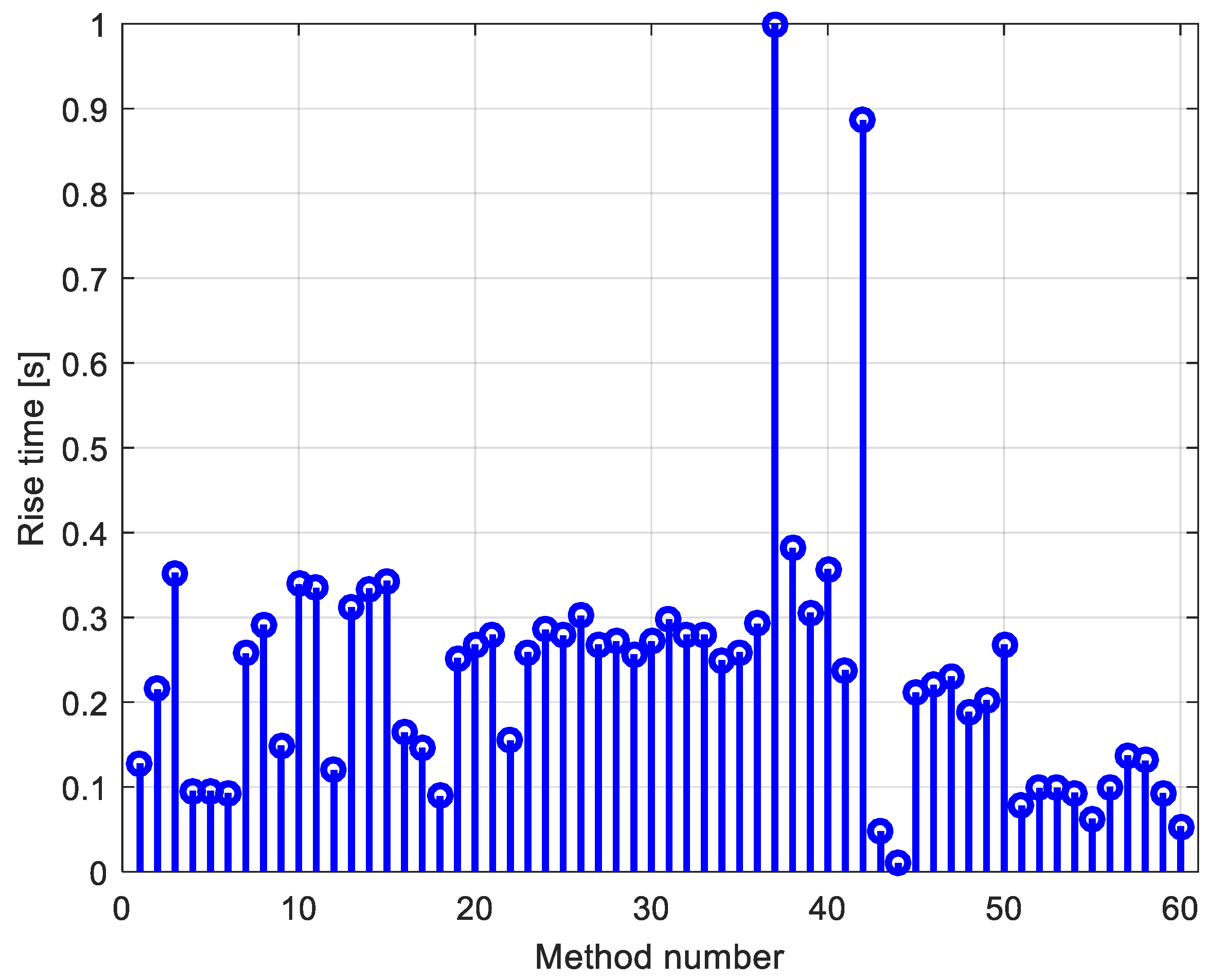
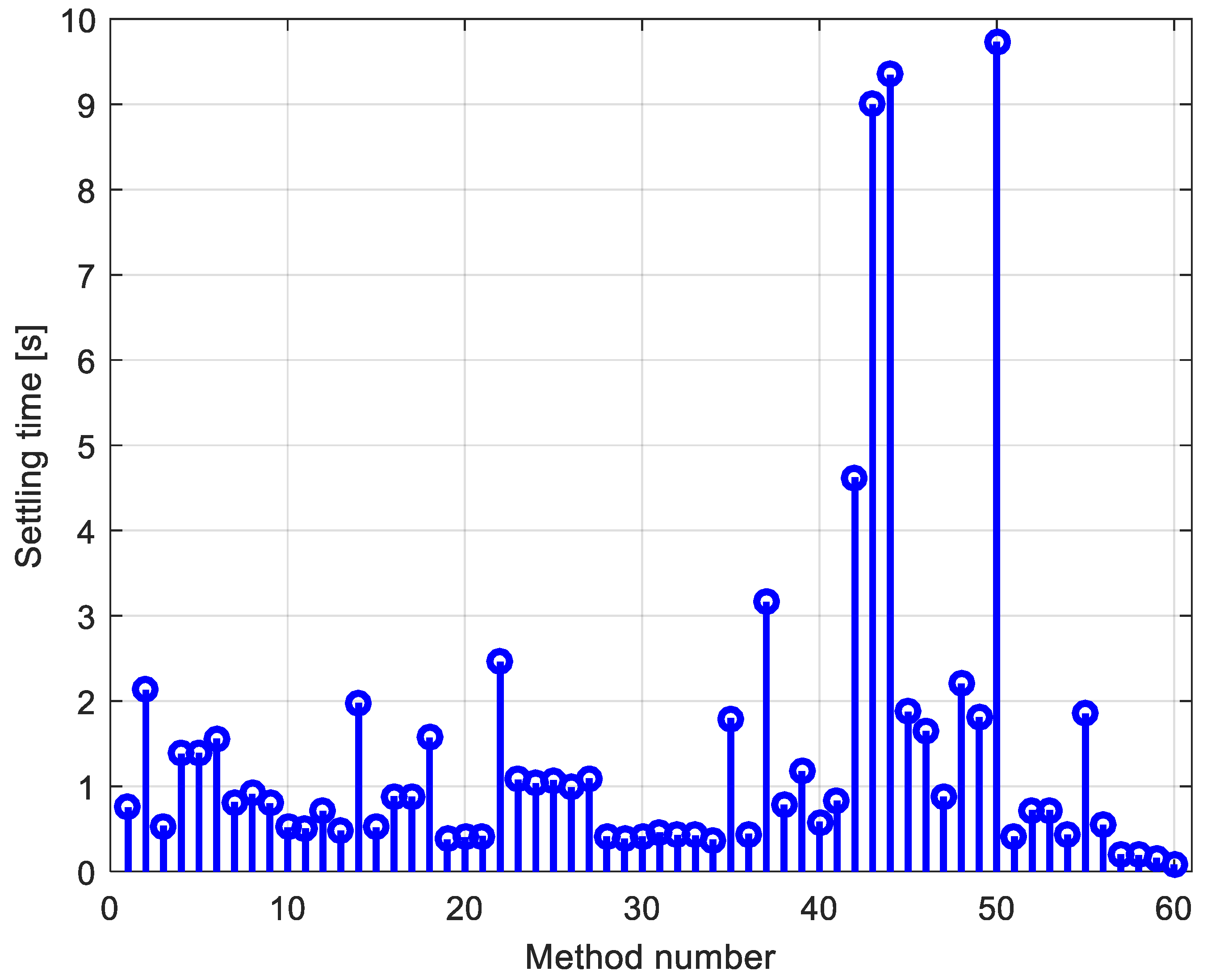
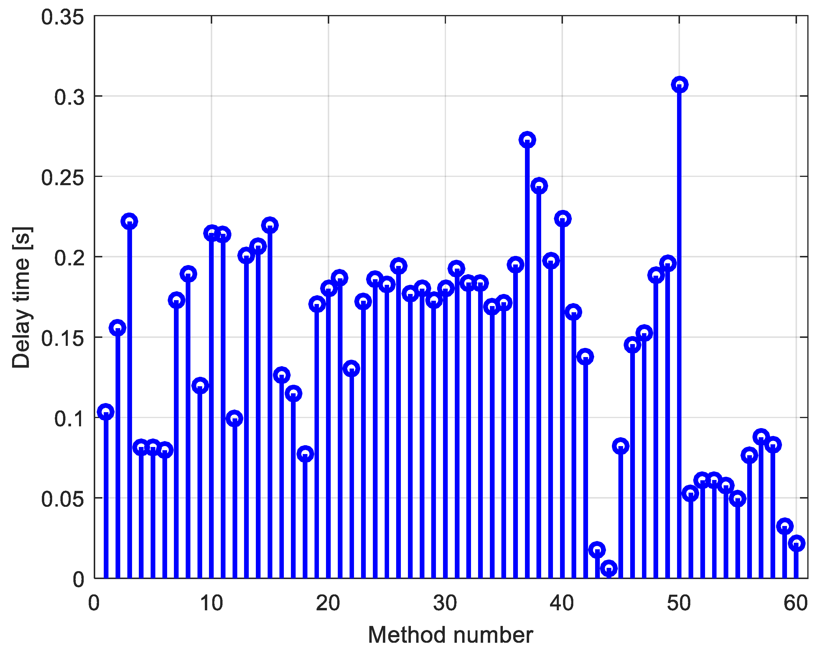
60	[17]		2.9943	2.9787	1.5882	-	-	-	0.102

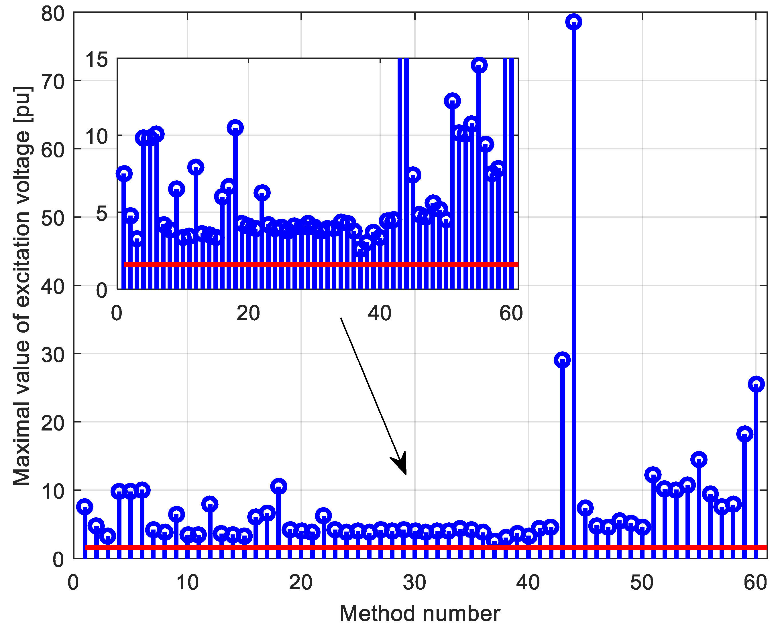
presents the optimal values of the parameters for different types of PID controllers (ideal PID, real PID, FOPID, and PIDD²) that are tuned by different algorithms. Using the presented data, different simulations were carried out to obtain step responses of the AVR system. A comparison of the obtained results, in terms of the rise time, delay time, overshoot, settling time, and maximum value of excitation voltage is presented in Figure 2, Figure 3, Figure 4, Figure 5 and Figure 6, respectively. For the presented results, it is clear that all the existing methods guarantee null steady state error. However, there are big differences in terms of the characteristic time metrics (overshoot, rise time, settling time), which means that these different methods do not provide the optimal PID design so far.

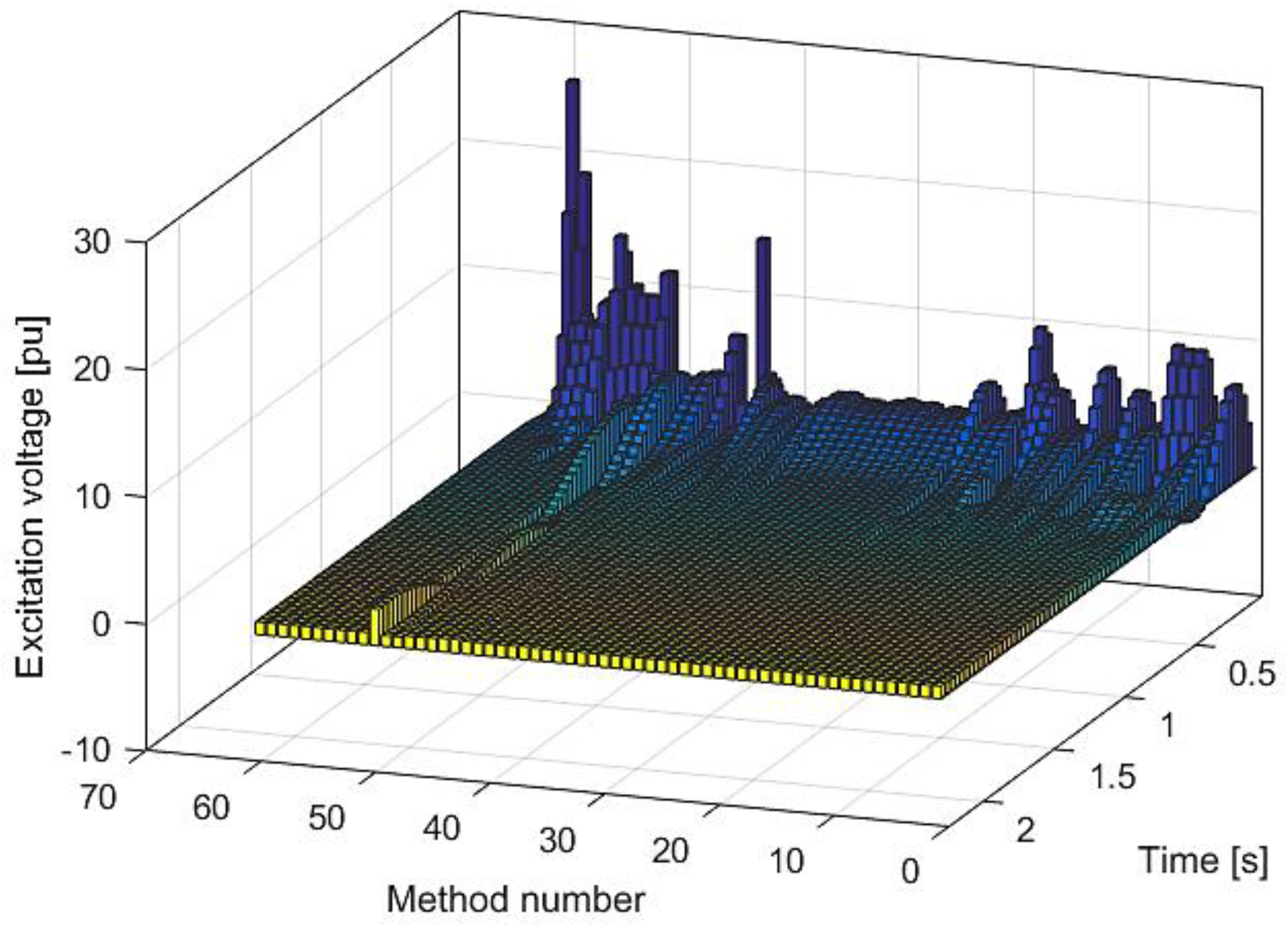
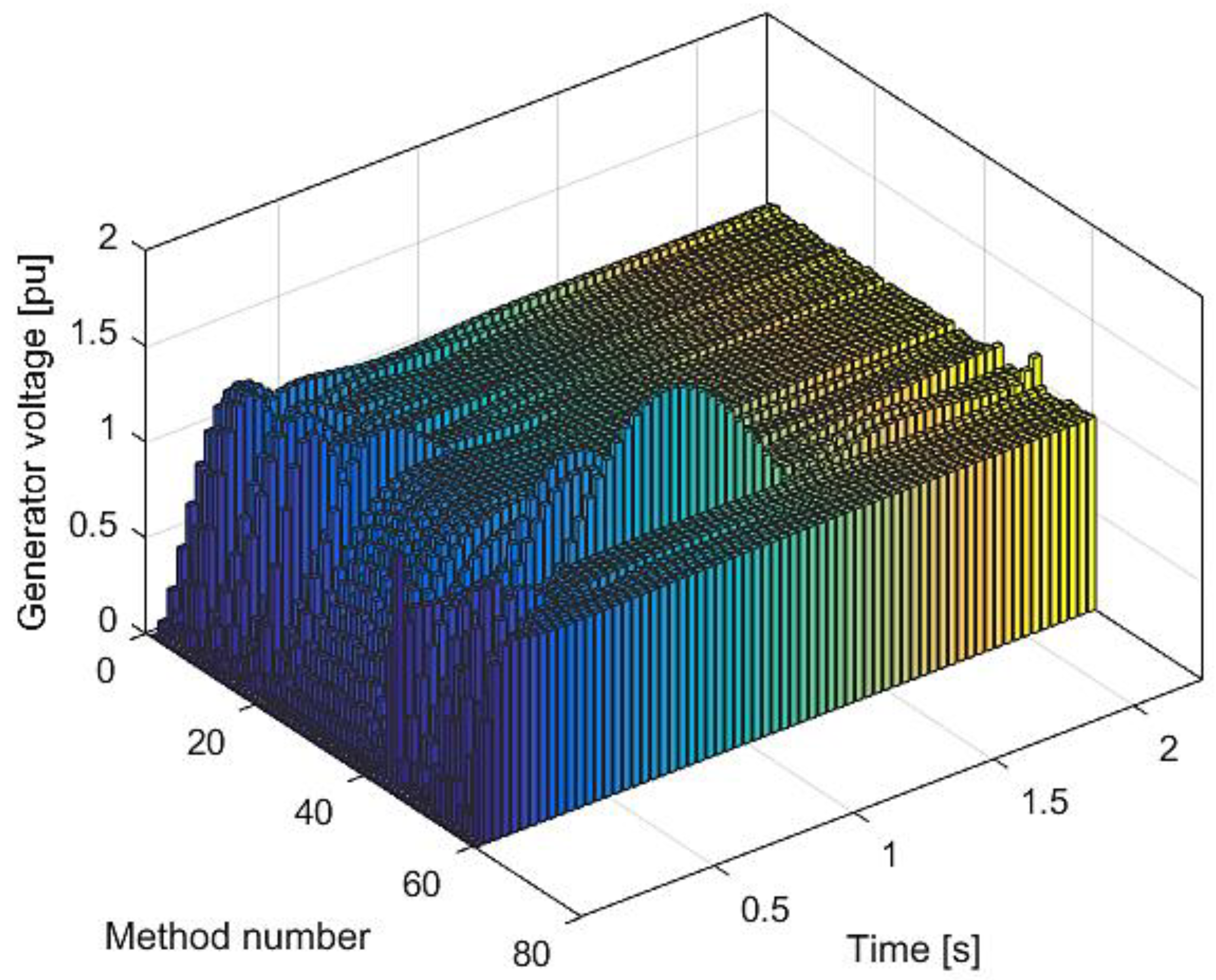
These differences can be better viewed on the 3D graphs presented in Figure 7 and Figure 8. These graphs are plotted with a time step of 0.03. Namely, in this figure, the generator and excitation voltage responses of the AVR system via different PID parameters obtained using the methods presented in Table 1 are shown.

It can be seen that the best system responses were using PIDD² compared to others. Additionally, it is more than evident that observing settling time, as well as overshoot are important time-domain parameters. Regarding the maximum value of the excitation voltage calculated via the different methods in Table 1, in all cases, the maximum value of the excitation voltage is higher than the permitted limit (limit is plotted with the bold line in Figure 6). For that reason, it can be concluded that the existing PID values do not guarantee a safe operation of the generator even at small voltage pulsations. For that reason, special attention to PID design should be paid if the investigated generator was operating in a weak network.

4. Equilibrium Optimizer–Evaporation Rate Water Cycle Algorithm

This article proposes a novel hybrid metaheuristic algorithm called equilibrium optimizer–evaporation rate water cycle (EO–ERWCA) algorithm for determining the optimal values of PIDD² controller parameters. In this regard, hybrid metaheuristic algorithms can be constructed using different hybridization strategies [34] based on populations, sub-populations, and individuals. The hybrid algorithm proposed in this paper belongs to the hybrid algorithms based on sub-populations. The main idea is to split the population into two sub-populations, and then separately apply the EO algorithm [35] on one sub-population and the ER-WCA algorithm [36] on the other sub-population. These algorithms have been chosen because of their extremely high efficiency in solving problems related to the estimation of the parameters [37,38]. General steps of such a hybrid algorithm are depicted in the following pseudo-code in Algorithm 1:

Algorithm 1 Hybrid EO-ERWCA Algorithm: Pseudo-Code

Pseudo-code of hybrid EO-ERWCA algorithm

Randomly initialize the population

Split the population into two sub-populations

for iterator = 1 to max_iterations

for m = 1 to population_size

Update the first sub-population using the EO algorithm

Update the second sub-population using ER—WCA algorithm

end for

end for

Determine the best individual from both sub-populations

4.1. EO Algorithm

The population consists of a certain number of individuals, denoted with N. In the EO algorithm, each individual is represented with its concentration, which stands for the potential solution of the optimization problem. Before the iterative procedure starts, the population of the algorithm is randomly initialized between the lower and upper bounds of the optimization variables. The concentration of each particle C at iteration ite is updated using Equation (8), and it depends on C_eq—equilibrium concentration, F—exponential term, G—generation rate, λ—turnover rate, V—volume (set to unity in this work), as follows:

$$C\left(ite\right)=C_{eq}+\left(C\left(ite-1\right)-C_{eq}\right)F+\frac{G}{\lambda V}\left(1-F\right)$$

(8)

→

The first term C_eq is called equilibrium concentration and it stands for the random concentration chosen from the equilibrium pool C_eq,pool. This pool consists of four best solutions after each iteration and their average value is formulated as follows:

$$\begin{array}{l}{C}_{eq,pool}=\left\{C_{eq(1)},C_{eq(2)},C_{eq(3)},C_{eq(4)},C_{eq(ave)}\right\},\\ C_{eq(ave)}=\frac{C_{eq(1)}+C_{eq(2)}+C_{eq(3)}+C_{eq(4)}}{4}.\end{array}$$

(9)

→

The second term consists of the difference between the concentration in the previous iteration and the current equilibrium concentration, scaled with exponential term F. This part of Equation (9) forces the global search of the algorithm, or so-called the exploration phase. The exponential term is defined as follows:

$$F=e^{-\lambda (t-t_0)}$$

(10)

where λ denotes the turnover rate and consists of random numbers in the range [0, 1]. The exponential term is also defined with vectors t and t₀, which are calculated as follows:

$$t={\left(1-\frac{ite}{max\_ite}\right)}^{a_2\frac{ite}{max\_ite}}$$

(11)

$$t_0=\frac{1}{\lambda }ln\left[-a_1\left(1-e^{-\lambda t}\right)\cdot sign(r-0.5)\right]+t$$

(12)

where max_ite stands for the number of iterations of the algorithm, a₁ and a₂ are constants whose values are set to 2 and 1, respectively, while r is a vector of random numbers in the range [0, 1].

→

The third term focuses on the local search of the algorithm, and is defined with the generation rate G, which is calculated using Equation (13):

$$G=G_0{e}^{-\lambda (t-t_0)}=G_{0}F$$

(13)

The initial value of the generation rate is denoted with G₀ and can be determined as follows:

$$G_0=G_{CP}\left(C_{eq}-\lambda C\left(ite-1\right)\right)$$

(14)

where G_CP stands for generation rate control parameter, whose value depends on generation probability GP, which is set to 0.5, and random numbers in the range [0, 1], denoted with r₁ and r₂.

$$G_{CP}=\{\begin{array}{l}0.5r_1,r_2\ge GP\\ 0,r_2<GP\end{array}$$

(15)

Finally, after reaching the selected number of iterations, the optimal solution of the EO algorithm is represented by the concentration of the individual with the lowest fitness function value.

4.2. ER-WCA Algorithm

The second sub-population is handled by the ER–WCA algorithm. Similar to the EO algorithm, the sub-population of the total population that belongs to ER–WCA algorithm is also randomly initialized between boundaries of the optimization variables. The population of ER–WCA algorithm consists of the sea, rivers, and streams. Precisely, there is one sea, the number of rivers is predefined with the parameter N_r, and the number of streams is determined with N_s = N_pop − N_r − 1, where N_pop stands for the population size. This algorithm is based on the water cycle process that normally occurs in nature. Namely, each stream in nature flows to the river or the sea. Therefore, the number of streams that belong to each river and the sea must be determined using Equation (16).

$$N{S}_n=round\left\{\left|\frac{C_n}{{\displaystyle \sum _{n=1}^{N_{sr}}{C}_n}}\right|N_s\right\},n=1,2,\dots ,N_{sr},\left(N_{sr}=N_r+1\right)$$

(16)

where NS_n denotes the number of streams that flow into the nth river or the sea if n equals 1 is assumed. In the previous equation, round{} stands for the rounding to the nearest integer number, while || denotes the absolute value. Additionally, C_n is calculated as follows:

$$C_n=f(X_n)-f(X_{N_{sr}+1}),n=1,2,\dots ,N_{sr}$$

(17)

where X_i represents the ith individual of the population, and f() stands for the fitness function. Each stream can flow to either river or sea. The mathematical formulations will differ depending on the final destination of the stream. If the stream flows into the river, its position that is denoted X_stream is updated using Equation (18). Thus:

$$X_{stream}\left(ite\right)=X_{stream}\left(ite-1\right)+rand\cdot C\left(X_{river}\left(ite-1\right)-X_{stream}\left(ite-1\right)\right)$$

(18)

The other possible situation is that the stream flows into the sea. In this case, the position of the corresponding stream is updated using Equation (19):

$$X_{stream}\left(ite\right)=X_{stream}\left(ite-1\right)+rand\cdot C\left(X_{sea}\left(ite-1\right)-X_{stream}\left(ite-1\right)\right)$$

(19)

In the previous equations, rand stands for a random number between 0 and 1 that is generated separately for each stream, while C is a predefined parameter that is selected to be 2, according to [36].

After the update procedure for each stream is finished, it is necessary to compare the fitness functions of such obtained streams and the corresponding river. If a certain stream has a lower value of the fitness function than the river, that stream becomes the river, and vice versa (their roles are switched).

A similar procedure is also carried out for the rivers. Namely, the position of each river is updated using Equation (20).

$$X_{river}\left(t\right)=X_{river}\left(t\right)+rand\cdot C\left(X_{sea}\left(t\right)-X_{river}\left(t\right)\right)$$

(20)

The fitness function of updated rivers must be calculated and compared with the fitness function of the sea. If a river has a lower fitness function value than the sea, their positions will be swapped.

The final stage of ER–WCA is the process of evaporation. The evaporation can occur in two cases:

→

Firstly, if the river has only a few streams, it can evaporate even before it reaches the sea. The chance of evaporation is defined with the evaporation rate (ER):

$$ER=\frac{sum(N{S}_n)}{N_{sr}-1}\cdot rand,n=2,3,\dots ,N_{sr}$$

(21)

If the evaporation occurs, the river disappears but the new stream is formed from the vapor, so that:

$$X_{stream}^{new}=LB+rand\cdot \left(UB-LB\right)$$

(22)

where LB and UB stand for the lower and upper bounds of optimization variables, respectively.

In summary, the evaporation process of the rivers can be summarized as follows:

$$\begin{array}{l}if\left(e^{-\frac{ite}{max\_ite}}<rand\right)\&\left(N{S}_i<ER\right),i=1,2,\dots ,N_r\\ X_{stream}^{new}=LB+rand\cdot \left(UB-LB\right);\\ end if\end{array}$$

(23)

→

Secondly, rivers and streams can flow to the sea. Afterward, the seawater will evaporate. The evaporation in the case when river flows into the sea is modeled as follows:

$$\begin{array}{l}if\left(\left|X_{sea}-X_i\right|<d_{max}\right)or\left(rand<0.1\right),i=1,2,\dots ,N_r\\ X_{stream}^{new}=LB+rand\cdot \left(UB-LB\right);\\ end if\end{array}$$

(24)

Similar to this, the evaporation of the seawater when the stream flows into the sea is described with Equation (25):

$$\begin{array}{l}if\left(\left|X_{sea}-X_i\right|<d_{max}\right),i=1,2,\dots ,N_s\\ X_{stream}^{new}=X_{sea}+\sqrt{\mu }\cdot randn;\\ end if\end{array}$$

(25)

where μ is a parameter, whose value is set to 0.1 [36]. Furthermore, randn(1, N) is a vector of standard Gaussian numbers, and d_max is a parameter that changes at each iteration, as follows:

$$d_{max}\left(ite\right)=d_{max}\left(ite-1\right)-\frac{d_{max}\left(ite\right)}{max\_ite}$$

(26)

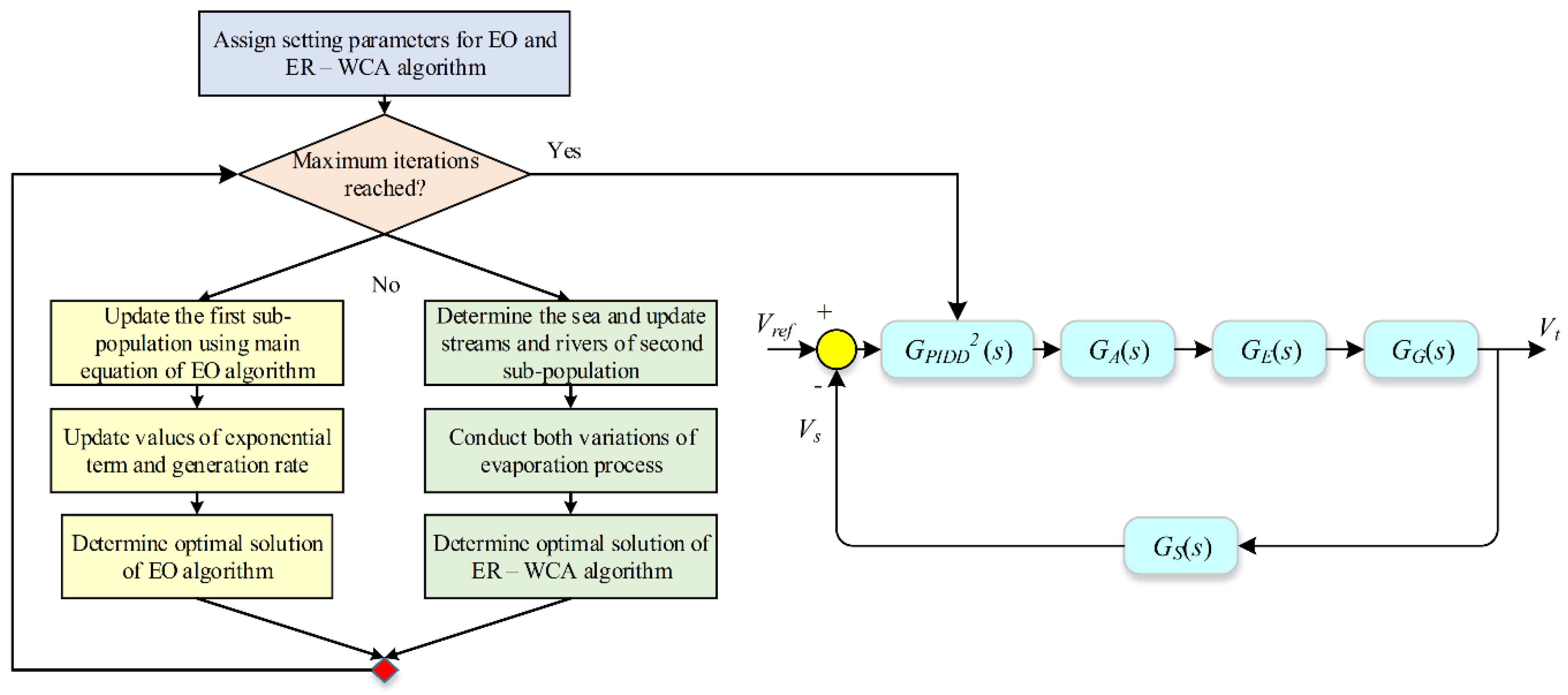
Finally, after the end of the evaporation process, one iteration of the ER–WCA algorithm is completed. The described process should be repeated until the maximum number of iterations is reached. Then, the individual with the lowest fitness function value stands for the optimal solution of ER–WCA algorithm. The global optimal solution of the problem is obtained by comparing the solution obtained from the first sub-population which is handled by the EO algorithm and the other solution from the second sub-population that is handled by the ER–WCA algorithm. The procedure of the hybrid EO–ERWCA algorithm for determining the optimal set of PIDD² controller parameters can be summarized by the flowchart presented in Figure 9.

The maximum number of iterations is the parameter that should be carefully chosen. It is important not to set this parameter to be too high because it will slow down the optimization process, but also it should not be too small because the optimal solution might not be reached. In this work, the maximum number of iterations is set to 100.

5. Simulation Results

The simulations presented in this paper were carried out in Matlab R2019b, on the computer with the following performances: processor Intel i7 1065G7 1.3 GHz, RAM memory 16 GB, and hard disk with the capacity of 500 GB.

Two objective functions are suggested for PID parameters design considering the excitation voltage/current limit, as follows:

$$O{F}_1=\{\begin{array}{ll}{\displaystyle \sum _{k=1}^N}{\left(V_R-V_g(k)\right)}^2& \mathrm{if}\max \left(V_{exc}\right)\le V_{exc}^{\mathrm{limit}}\\ \infty & \mathrm{if}\max \left(V_{exc}\right)>V_{exc}^{\mathrm{limit}}\end{array}$$

(27)

$$O{F}_2=\{\begin{array}{ll}{\displaystyle \sum _{k=1}^N}{\left(V_R-V_g(k)\right)}^2+10\cdot \max \left(V_g\right)& \mathrm{if}\max \left(V_{exc}\right)\le V_{exc}^{\mathrm{limit}}\\ \infty & \mathrm{if}\max \left(V_{exc}\right)>V_{exc}^{\mathrm{li}\mathrm{mi}t}\end{array}$$

(28)

Therefore, PID parameter design includes instantaneous tracking of the excitation voltage value due to the generator reference voltage change. If the instantaneous value of the excitation voltage at any point k is higher than the maximum allowed value of the excitation voltage ($V_{exc}^{\mathrm{limit}}$), the value of the objective function will be equal to infinity. If for all measured points the excitation voltage is lower than the maximum allowable value of the excitation voltage, the objective function shall be calculated as a summation of the squared value of the absolute error (OF₁) or as a summation of the squared value of the absolute error and the maximum value of the generator voltage multiplied by gains. After a lot of simulations and tests, it was found that the optimal value of the gain is 10. Therefore, the used PID parameters cannot lead to impermissible excitation voltage values upon the reference voltage change.

During the optimization process, the maximum and minimum value of PID parameters are defined to be in pre-specified limits (for all parameters, the lower value is 1 × 10⁻⁵, while the upper value is 1).

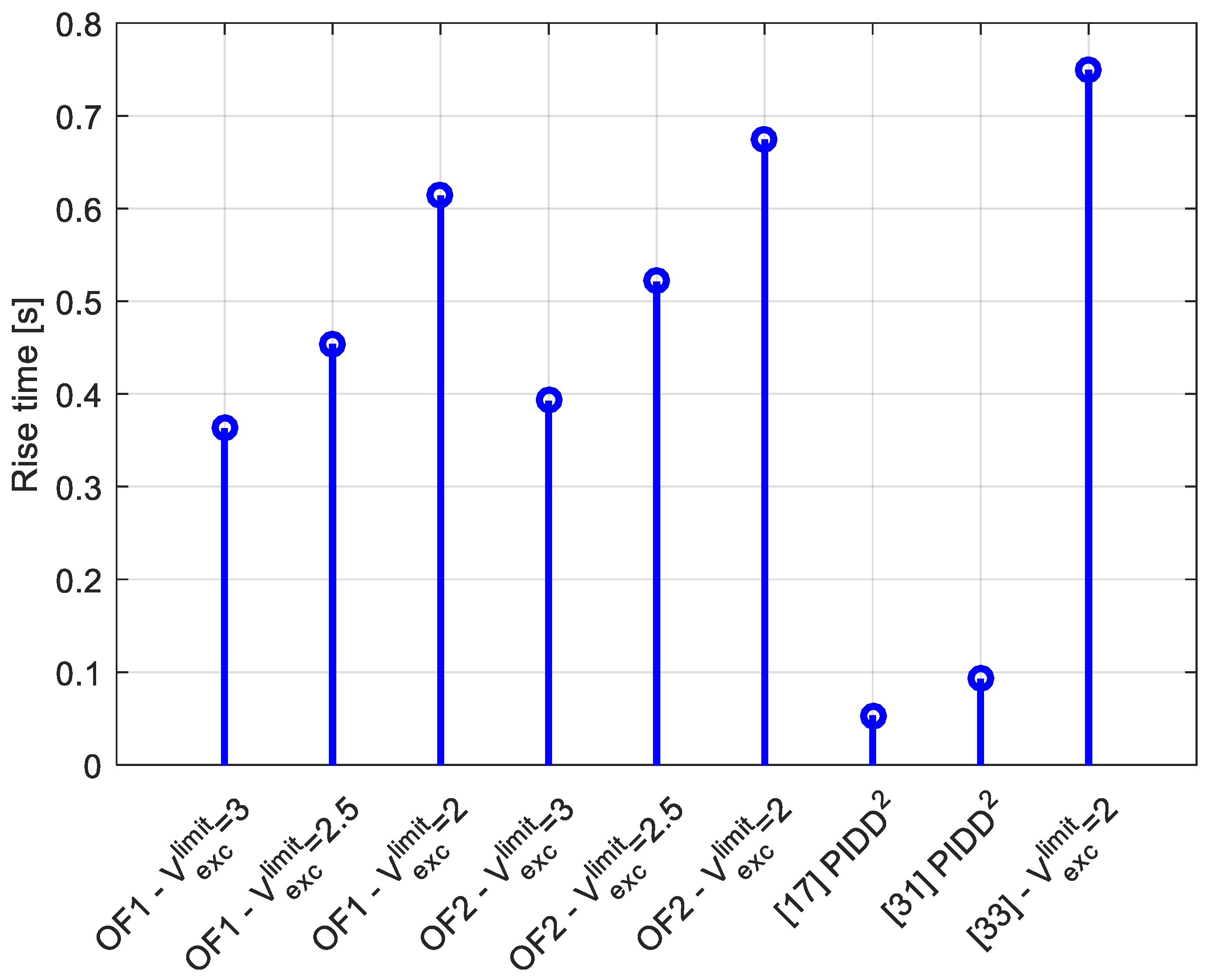
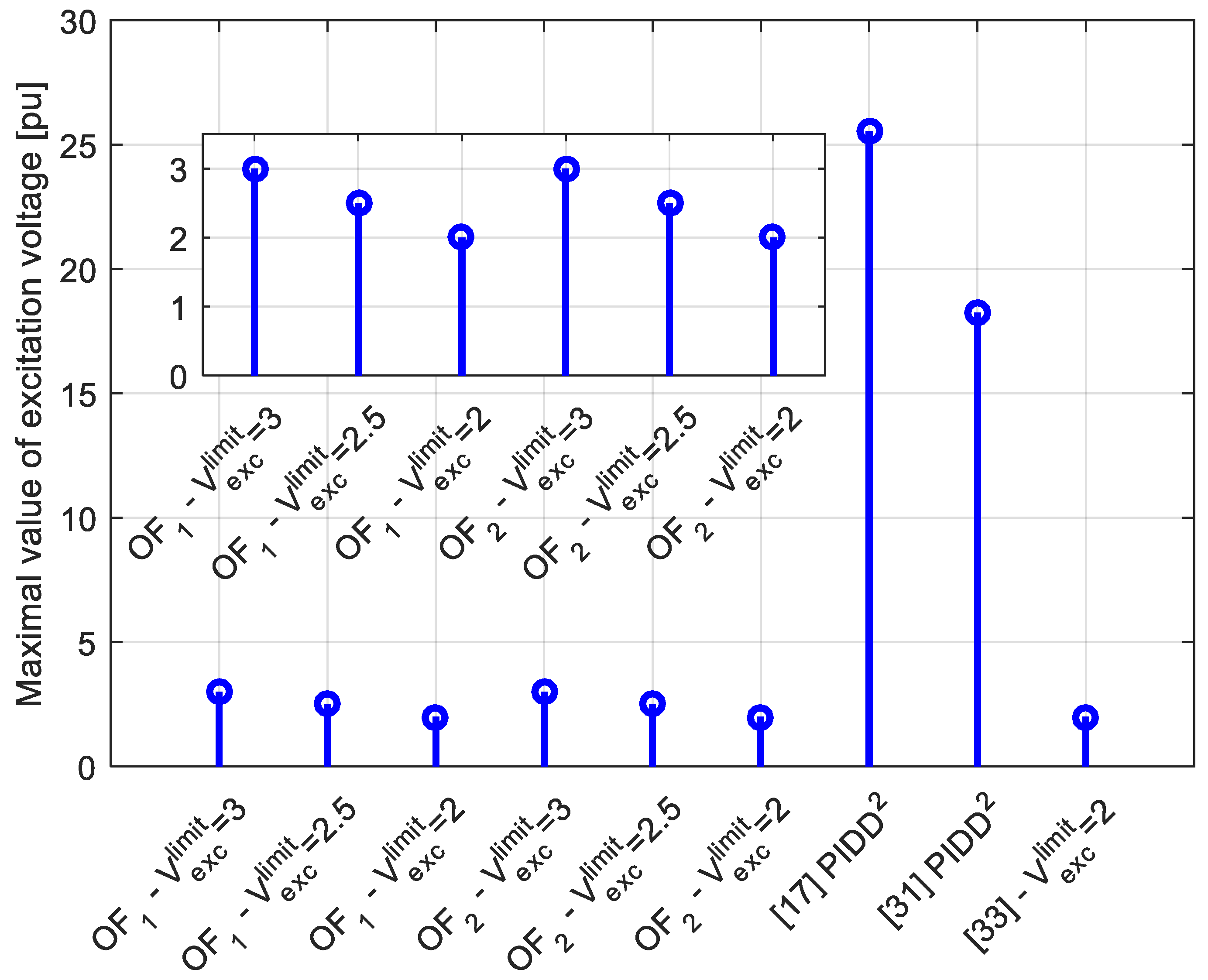
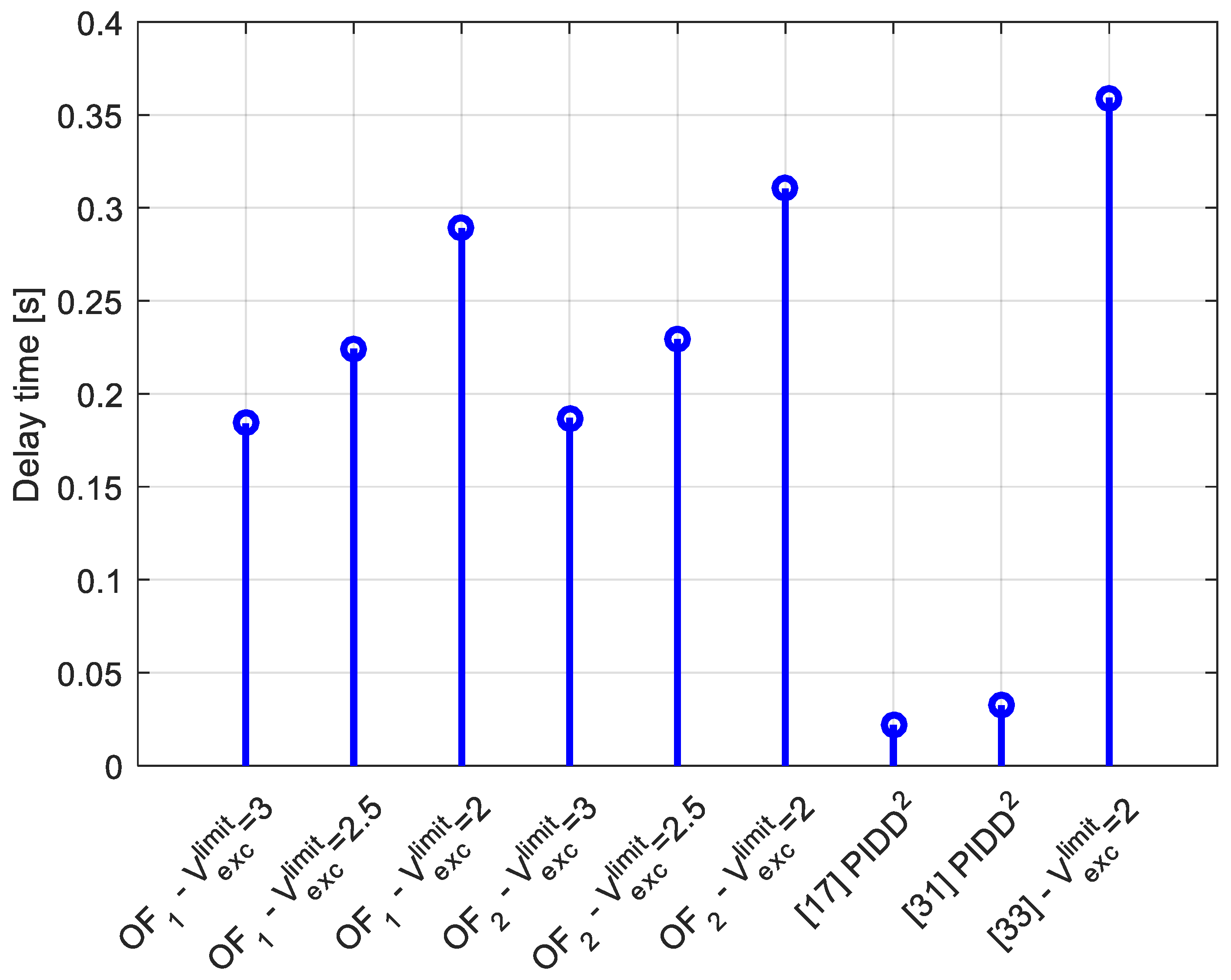
The optimal PID parameters obtained using the proposed algorithm for different values of the excitation voltage limit, for both objective functions, are presented in

Table 2. Comparison of the results obtained using the proposed and presented algorithms in the literature.

Methods	Excitation Voltage Limit (p.u)	Regulator	kp	ki	kd	kd2
OF1 via the proposed method	3.0	PIDD2	0.8577	0.4361	0.1783	0.0116
	2.5		0.6531	0.3624	0.1428	0.0098
	2.0		0.4498	0.3137	0.1104	0.0079
OF2 via the proposed method	3.0	PIDD2	0.7407	0.4396	0.1859	0.0109
	2.5		0.5459	0.3435	0.1503	0.0092
	2.0		0.3809	0.2899	0.1079	0.0051
[17]	-	PIDD2	2.9943	2.9787	1.5882	0.102
[31]	-	PIDD2	2.7784	1.8521	0.9997	0.073
[33]	2.0	PID	0.2956	0.2625	0.0937	-

. The maximum value of the excitation voltage, values of the rise time, delay time, and overshoot are presented in Figure 10, Figure 11, Figure 12 and Figure 13, respectively.

Few investigations can be derived by observing these figures. Firstly, it can be seen that all parameter values enable null-stationary error. Secondly, smaller values of the excitation voltage limit lead to lower values of the parameters of the regulator. However, a lower value of the maximum excitation voltage increases the rise time and delay time values. Additionally, the parameters obtained using OF₂ enable a lower value of overshoot compared to the value obtained using the first objective function. Finally, compared to the PIDD² parameters in [17,31], it can be seen that the proposed design guarantees the secure and safe value of the excitation voltage. In addition, compared to the PIDD² parameters in [33], it can be seen that the proposed regulator design enables faster generator voltage change. Hence, it can be concluded that the proposed PIDD² is successfully realized.

5.1. Robustness of the AVR System

Three investigations were performed in this work to check the robustness of the AVR system with the proposed PIDD² parameters.

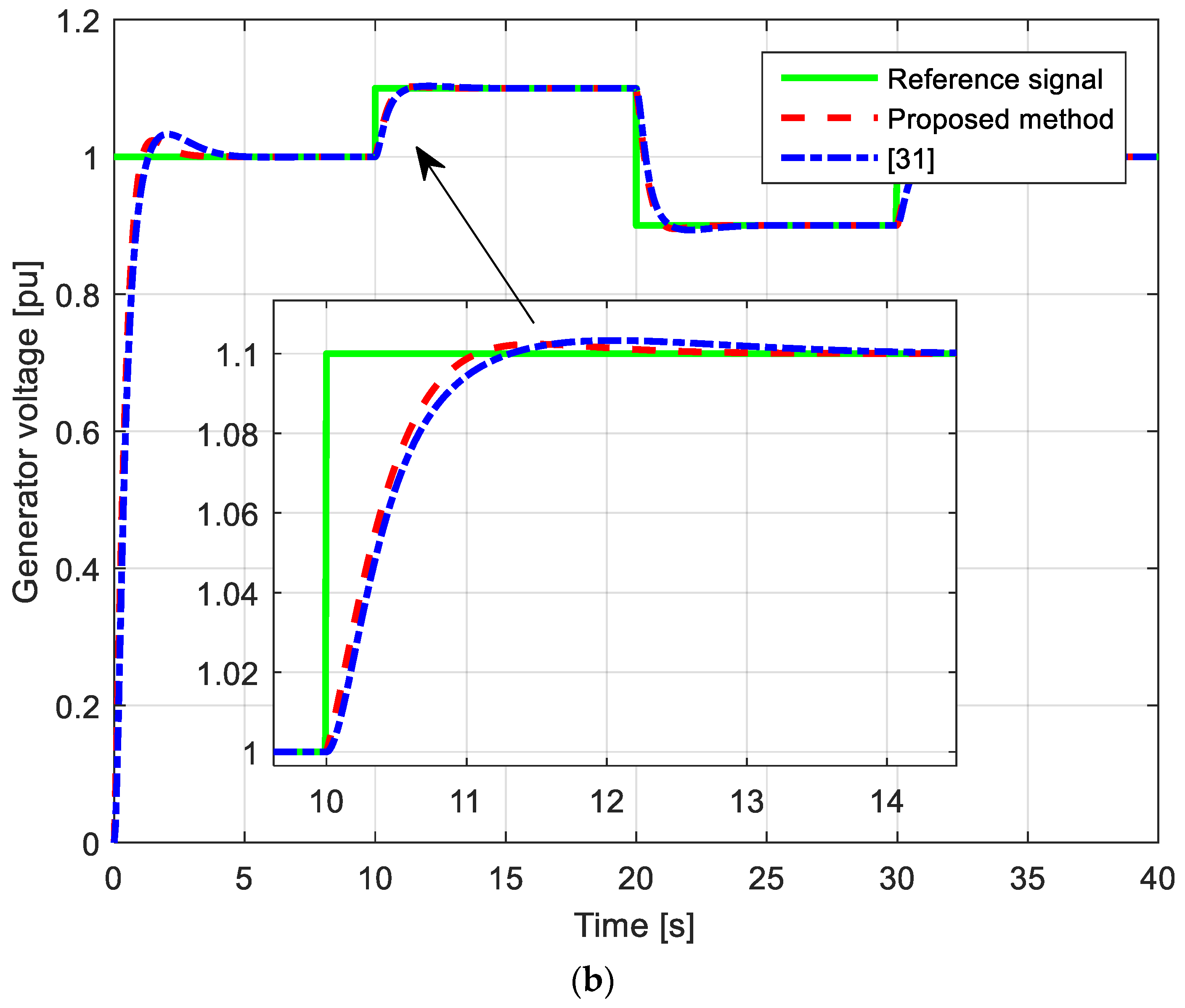
First, a set-point variation of the generator voltage is performed. Initially, the generator set-point equals 1 p.u, and after 10 s, it is set to 1.1 p.u, then after 20 s, it is set to 0.9 p.u, and finally, after 30 s, it returns to 1 p.u. The corresponding results are presented in Figure 14. Notably, the parameters obtained via OF₂ and using $V_{exc}^{limit}=2 \mathrm{p}.\mathrm{u}$are used. The PID parameters from [31] have provided a slower generator voltage response with a higher overshoot compared to the response obtained using the proposed controller. For both responses, the excitation voltage changes are within allowable limits.

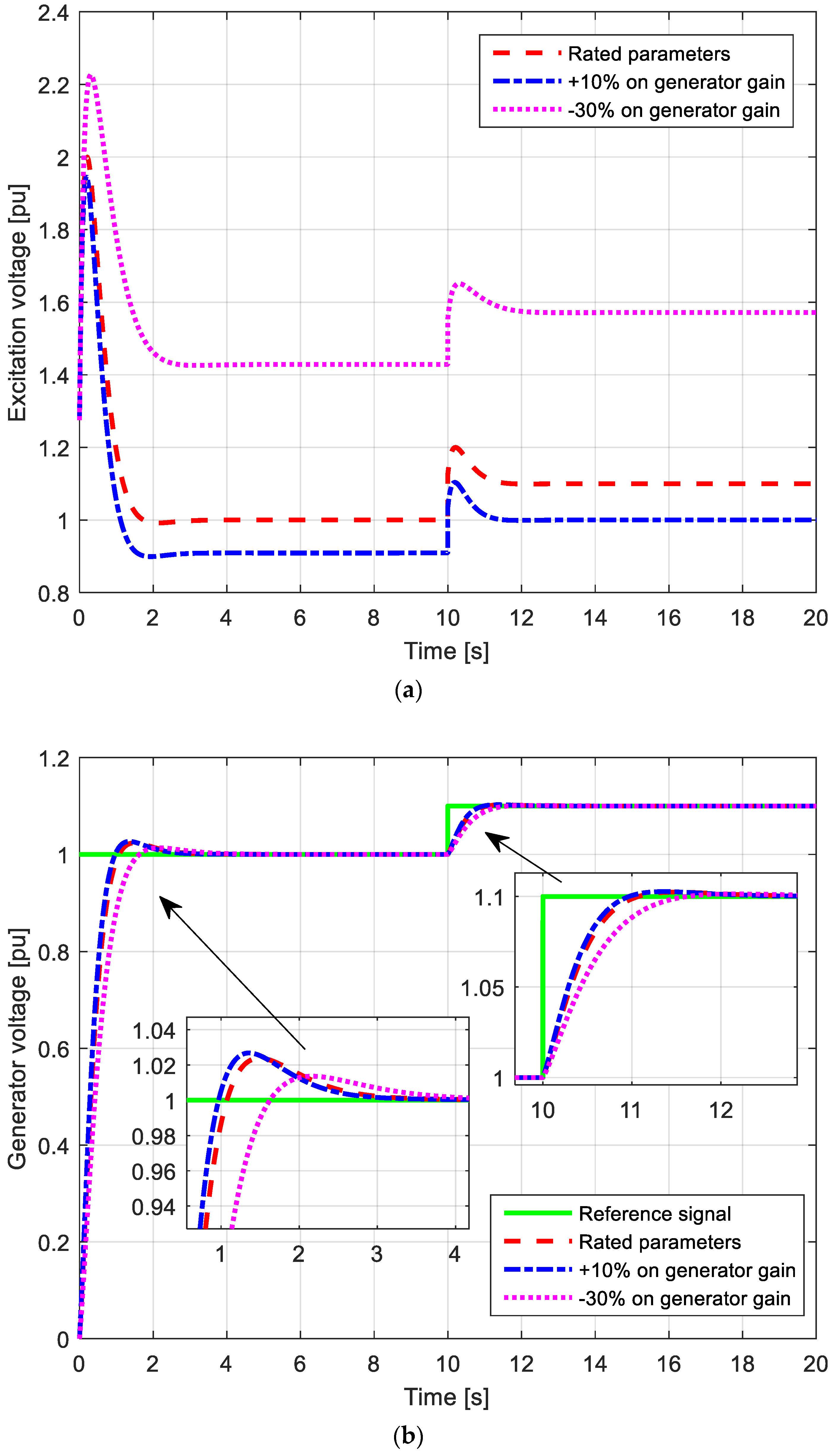
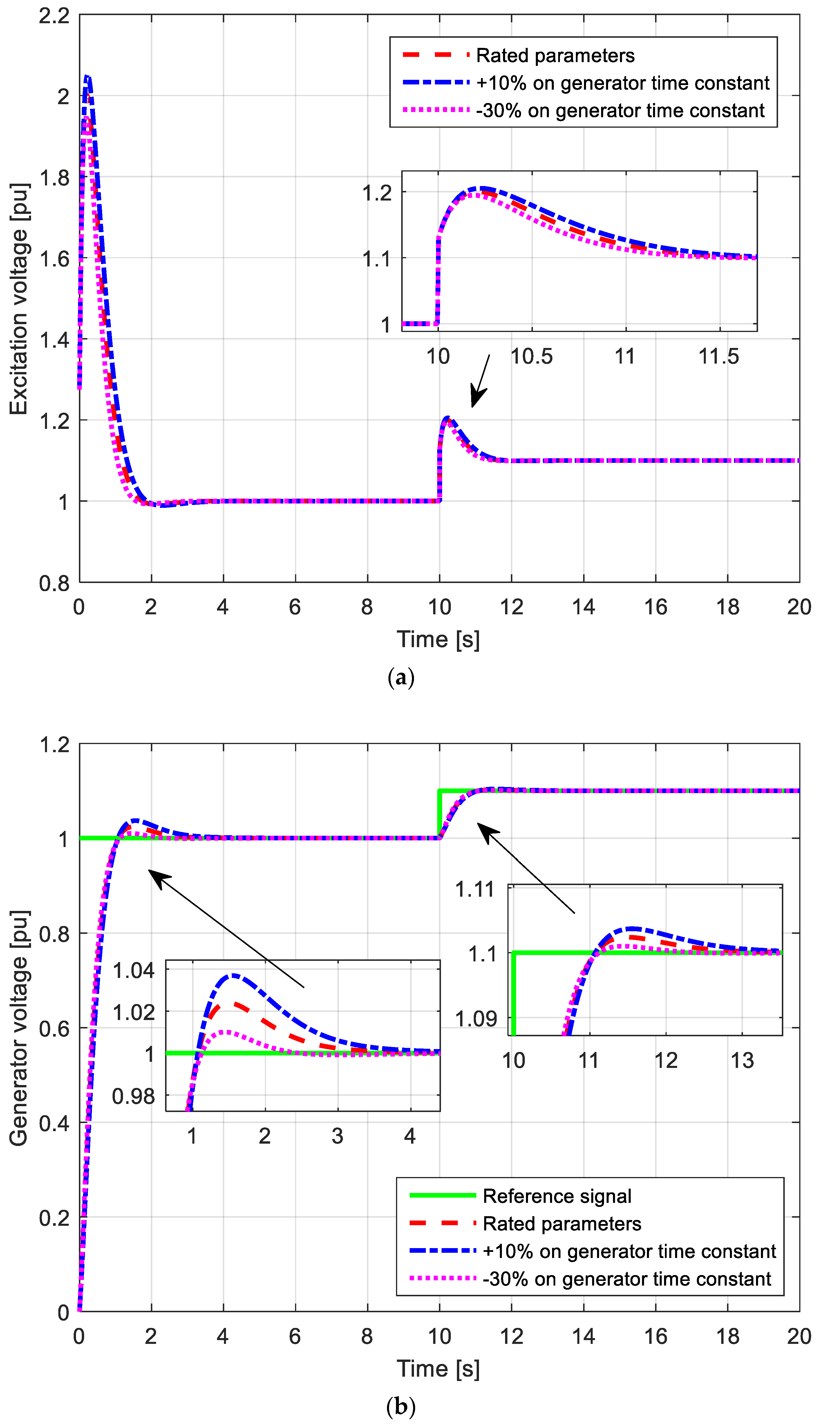
Second, the robustness is investigated by changing the generator gain and time constants. Figure 15 demonstrates the results for the base value (100%), 110%, and 70% of the generator gain. It should be noted that the value of the generator gain represents the value of the generator load [5,6,7,8,9,10,11,12,13,14,15]. The same results, for a change in the generator time constant (+10% and −10%) are presented in Figure 16. The results obtained show that the generator voltage change has a null stationary error. Additionally, the system is stable, while the excitation voltage rise is lower by 10% for a 10% rise of the generator gain. Therefore, according to these results, it can be seen that the controller parameters tuned by the proposed method provide the desired control behavior even in case of a change of a load of the generator.

Third, the robustness is checked by adding disturbance signals to the generator voltage, in which a positive and negative disturbance step signal (step signal whose value is 0.1 p.u) is added to the generator voltage value. The corresponding results are presented in Figure 17. It can be seen that the positive disturbance signal leads to a decrease in the excitation voltage, and vice versa. In addition, it is evident that on both disturbances (positive and negative), after the transitional process, the generator voltage comes into its steady state condition (1 p.u).

Finally, based on the results in all the scenarios conducted to investigate the robustness of the proposed PIDD² controller, it is clear that the proposed controller design enables stable and secure tracking of the reference signal as well as a reliable disturbance attenuation capability.

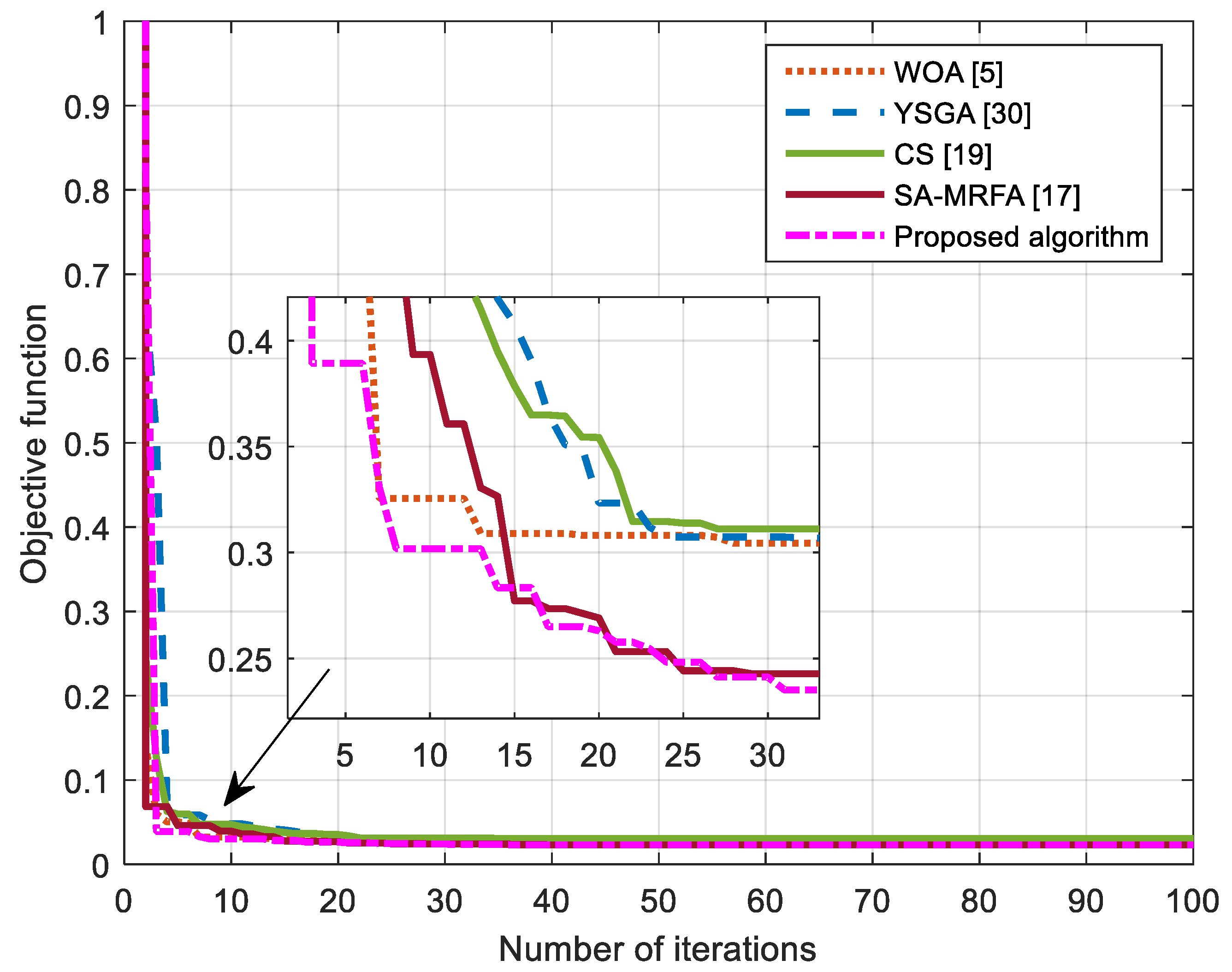
5.2. Algorithm Tests

All previously determined results (PIDD² design) were realized using the proposed EO–ERWCA algorithm. To demonstrate its power and superiority over other algorithms, a comparison between the proposed algorithm and other algorithms in the literature (WOA [5], YSGA [30], CS [19], and SA-MRFA [17]) is made in terms of the convergence speed. The number of runs in all algorithms was set to 30, and the normalized mean value of the convergence curves is presented in Figure 18. Additionally, each algorithm was employed to the optimal tuning of the real PID controller using the same settings as the proposed algorithm. It is obvious in Figure 18 that the EO-ERWCA converges to the optimal solution faster than other algorithms.

Moreover, it is well known that metaheuristic algorithms have a stochastic nature. For that reason, the considered algorithms had 30 independent runs and the best, worst, mean, and median values are calculated and presented in

Table 3. Statistical measures of the results obtained with the different algorithms.

Algorithm	Best	Worst	Mean	Median	Standard Deviation
EO-ERWCA	1284.5	1406.9	1345.1	1343.0	35.7286
YSGA	1284.7	1468.6	1378.4	1381.3	54.2141
CS	1284.6	1592.0	1429.7	1427.2	110.1038
WOA	1286.4	1530.8	1415.7	1424.6	70.0808

. Additionally, the standard deviation of the presented results was calculated. It is clear from Table 3 that the standard deviation has the lowest value when the proposed EO-ERWCA algorithm is applied. It can be concluded that the deviation of the results obtained from each run is very small, so the results obtained are consistent. In addition to the previous statistical analysis measures, a non-parametric statistical test called Wilcoxon’s rank-sum test was also carried out. This test enables additional comparison between the proposed EO–ERWCA algorithm and CS, WOA, and YSGA algorithms. The corresponding p-values obtained by applying this test are presented in

Table 4. p-Values obtained with Wilcoxon’s rank-sum test.

Algorithms	EO–ERWCA vs. CS	EO–ERWCA vs. WOA	EO–ERWCA vs. YSGA
p-value	4.4034 × 10−20	3.1748 × 10−19	3.3537 × 10−12

with a 5% level of significance between the EO–ERWCA and other optimization methods. The proposed algorithm is clearly effective, fast, and accurate.

6. Experimental Results

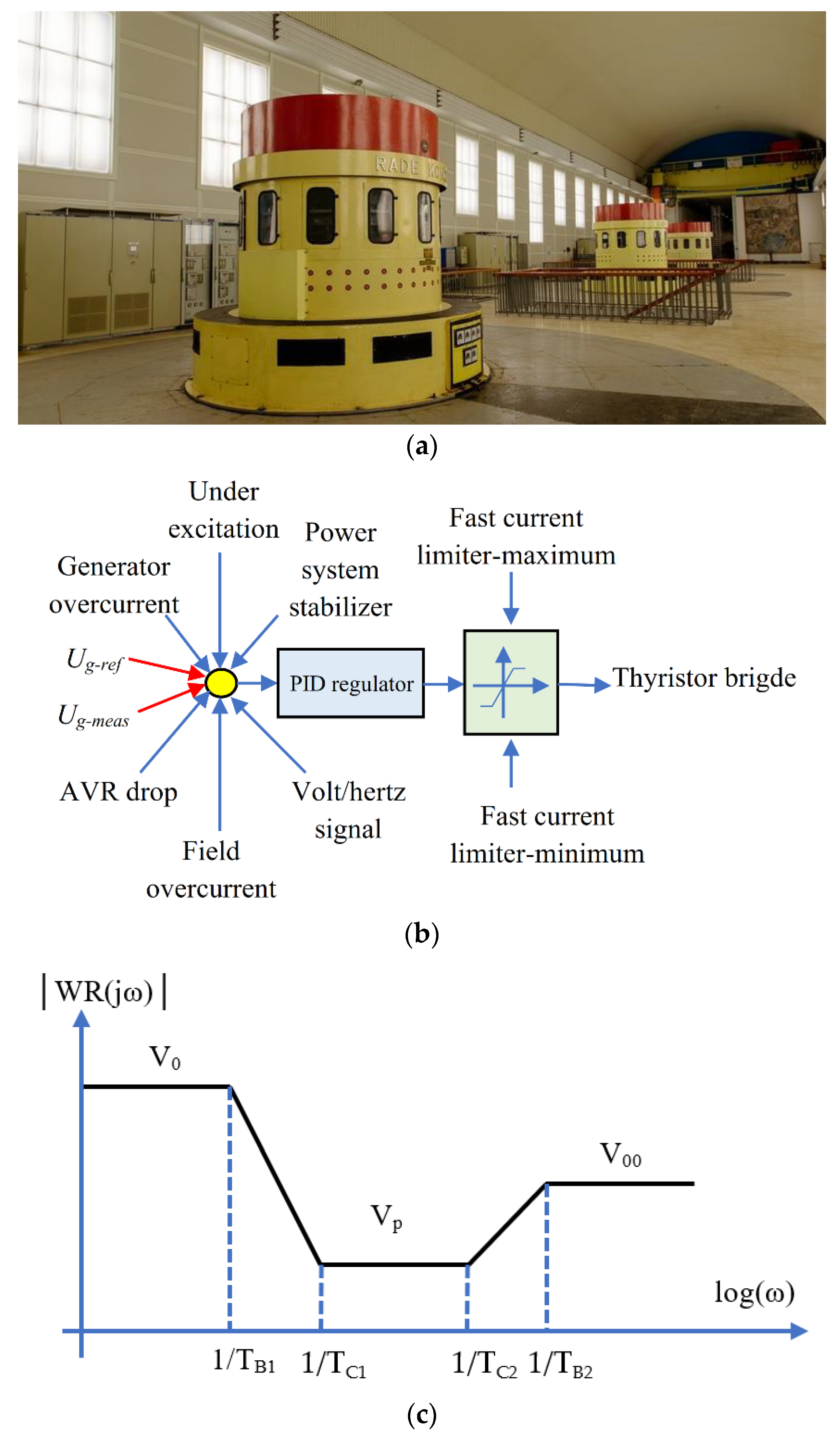
The previously presented simulations show that the limitation of the excitation voltage leads to a slower generator voltage change. In addition, the lower values of the regulator parameters provide a lower value of the excitation voltage. These analyses were the starting point for an experimental investigation of the proposed controller design. The experimental verification of the impact of excitation controller parameters value as well as of the excitation voltage value on the generator voltage was realized using a lead-lag compensator on one 120 MVA 15.75 kV, 50 Hz generator from HPP Piva, Montenegro, as shown in Figure 19a. The excitation system in HPP Piva is called Thyricon, which is manufactured by Voith Siemens. It is a thyristor-controlled self-excitation system. The control of the excitation voltage, besides the voltage control loop, includes other control loops such as excitation current, power system stabilizer, generator current, and others. In that way, the regulation of the generator voltage includes all the vital control variables. The regulation of the generator voltage was realized using a lead-lag compensator. The block diagram of the AVR control is presented in Figure 19b, where U_g-ref represents the generator reference value, while U_g-meas represents the generator measured voltage.

The lead-lag compensator, whose transfer function is WR(s), is realized in the following manner:

$$WR\left(s\right)=\frac{1+sT{C}_1}{1+sT{B}_1}\times \frac{1+sT{C}_2}{1+sT{B}_2}\times \frac{KR}{GR}$$

(29)

where TB_1,2 and TC_1,2 are time constants, KR is the proportional gain, and GR is the gain of the rectifier. The corresponding Bode characteristic of the lead-lag compensator is presented in Figure 19c.

These parameters are expressed as follows:

$$\begin{gathered} KR = V_0, T{B}_1 = \frac{T_a}{\raisebox{1ex}{$V_0$}\!\left/ \!\raisebox{-1ex}{$V_p$}\right.} \\ T{C}_1 = T_a, T{B}_2 = \frac{T_b}{\raisebox{1ex}{$V_p$}\!\left/ \!\raisebox{-1ex}{$V_{00}$}\right.}, T{C}_2 = T_b \end{gathered}$$

(30)

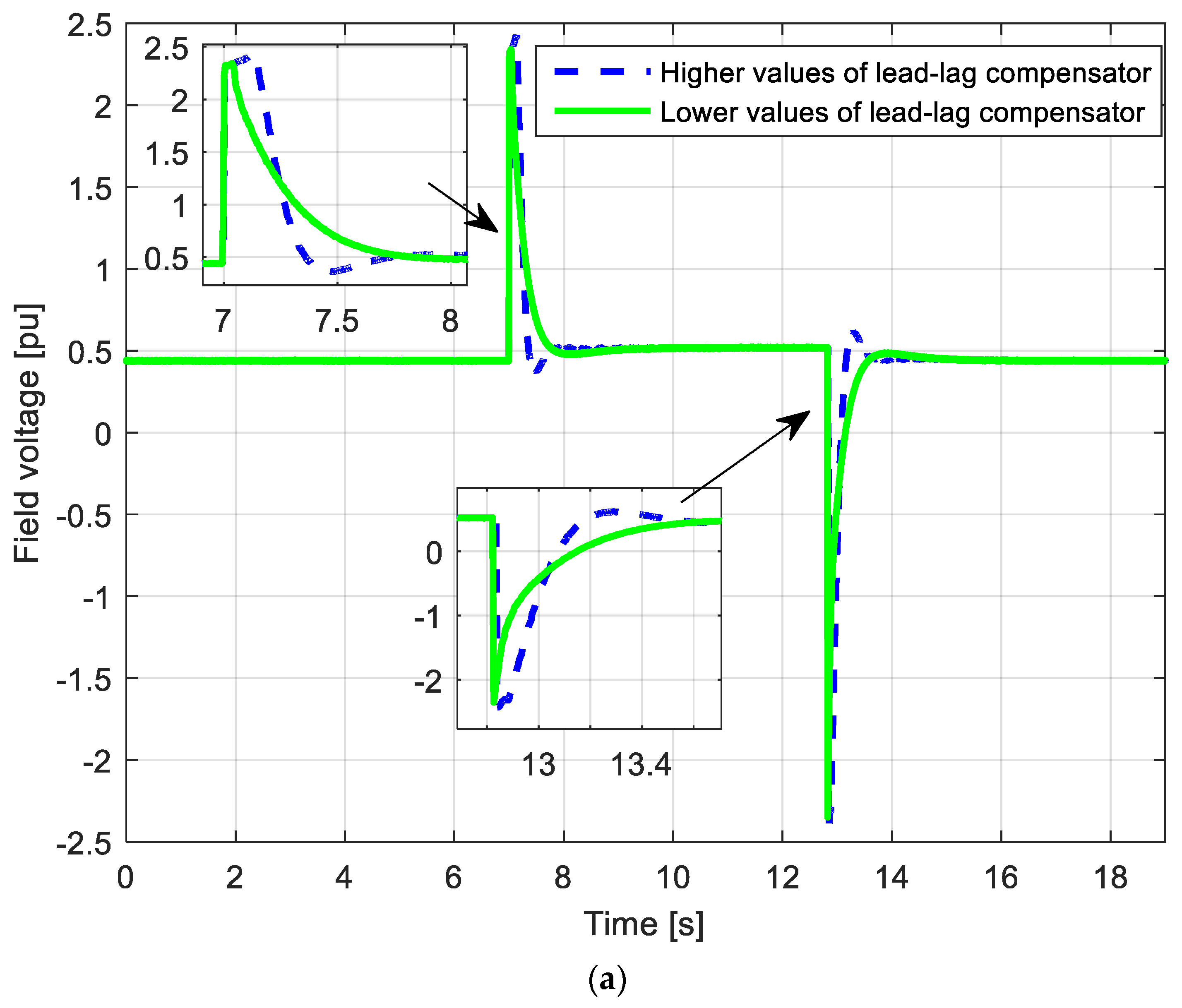
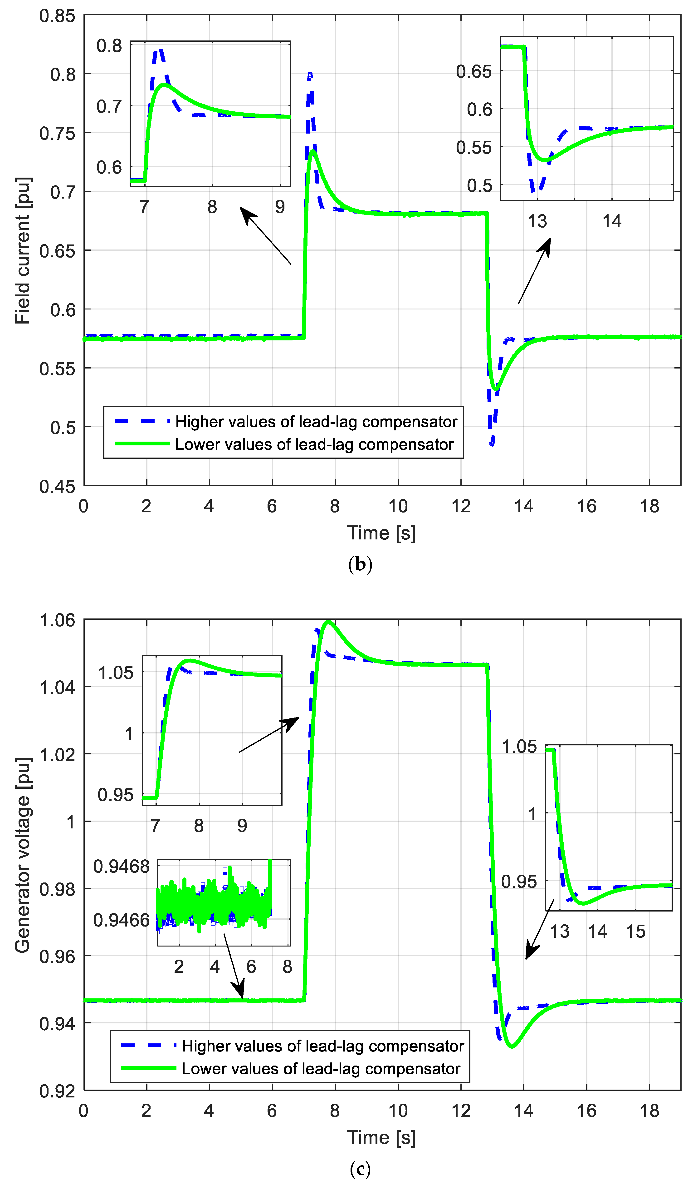
The generator is accelerated at the nominal speed and excited in no-load operation with a 0.947 p.u voltage value. After 7 s, the reference generator voltage set-point is changed to 1.046 p.u. A command is added to the excitation voltage to increase the generator voltage. Finally, after 6 s, the reference generator voltage is changed to the first value (0.947 p.u). This experiment is realized for two different values of lead-lag compensator parameters. In the first experiment, the lead-lag compensator parameters are T_a = 1.5 s, T_b = 0.1 s, V_p = 60, V₀ = 250, and V₀₀ = 50. In the second experiment, the lead-lag compensator parameters are T_a = 0.75 s, T_b = 0.05 s, V_p = 30, V₀ = 250, and V₀₀ = 50. The measurements were realized during July 2020 and refined in October 2021. For recording measurements, UNITROL UN6080 (SW version: 2.1.0.8), type: A6T-A/08T1-A1250, UN 6080 2CH was used. The corresponding results are presented in Figure 20.

The sudden change of the generator voltage set-point leads to a sudden rise of the excitation voltage. This very fast change enables the thyristor bridge operation in the static excitation system. The rise of the excitation voltage leads to the rise of the excitation current, and finally leads to the rise of output generator voltage.

On the opposite side, when the generator voltage set-point suddenly decreases, the excitation voltage suddenly decreases, which results in a reduction of the excitation current and voltage at the ends of the generator. In the second experiment, as lower lead-lag compensator parameters are implemented, the voltage response of the generator was slower. This is a consequence of the slower and smaller growth of the excitation current. Furthermore, in this case, forcing the field current after the initial rise was slower, as illustrated in Figure 20b. Therefore, the lower value of lead-lag compensator parameters provides a slower change of the generator voltage. It was also clear that higher values of lead-lag compensator parameters, i.e., a higher value of the excitation voltage causes smaller rise time and settling time of the generator voltage during step change. To sum up, it can be concluded that the value of lead-lag compensator parameters has considerable effects on the excitation voltage, excitation current, and generator voltage waveforms.

7. Conclusions

This paper addressed the design of regulators in AVR systems, as well as the experimental verification of the impact of the optimal regulator parameters on the generator. To this end, the importance of taking the value of the excitation voltage into account when designing parameters of the AVR system controller was first discussed. Additionally, a comparison of system responses of different controller parameters found in the literature was performed. Analyzing the obtained results, it was concluded that the PIDD² controller allows the minimum delay time and rise time of the generator voltage. Therefore, the parameters of the PIDD² controller were estimated and the excitation voltage values were monitored. Besides, two new optimization functions and a novel hybrid metaheuristic algorithm are proposed in the paper. Analyzing the obtained results using them, it was concluded that limiting the values of the excitation voltage leads to a decrease in the values of the optimal parameters of the regulator. Based on this conclusion, the influence of the values of the regulator parameters on the response of the excitation voltage and the generator voltage in HPP Piva was investigated. The experimental results validated the conclusions figured out from the simulation studies that limiting the maximum value of the excitation voltage leads to a higher value of the rise time and the rise time of the generator voltage. Finally, the determination of AVR controller parameters by applying the anti-windup type of excitation voltage limitation will be considered in future works.

In future work, the parameters of synchronous generators of HPP PIVA will be estimated to simulate the AVR system for generators of the same power plant. In this way, it will be possible to easily test different types and values of regulator parameters to achieve the desired generator voltage responses.