Kinematics Analysis and Optimization of a 3-DOF Planar Tensegrity Manipulator under Workspace Constraint

Abstract

Tensegrity mechanisms (TM) are well-appraised for their compliance and lightweight, making their design theory a hot research topic recently. However, due to unconstrained DOFs, the design and analysis of TMs are generally more complicated than traditional mechanisms composed of rigid links and joints. A compact 3-DOF tensegrity manipulator is introduced and an advanced two-step kinematic modeling method is proposed in this paper. This method is first assumed that bars and cables are rigid to estimate the equilibrium state using the energy-based method. Then, the flexibility of bars and cables is considered, and the force density method equations are solved utilizing the equilibrium state obtained by the previous step as the initial guess of iteration for fast computation. Based on the two-step method, the performances of the TM, such as workspace, manipulability, potential energy, and stiffness, are analyzed. Thereafter, the installation position and size of the manipulator are optimized under the workspace constraint. In the optimization process, discrete points on the prescribed task workspace contour are used to simplify the constraint to improve computational efficiency. Finally, study cases are investigated to validate the proposed method, and the feasibility of the discrete sampling method for constraint simplification is also verified.

1. Introduction

The word Tensegrity (tensile-integrity) was first proposed by Fuller [1] to describe a structure only containing compression members (struts) and tension members (cables or springs). As a structure characterized by self-stressing and high strength-to-weight ratio, tensegrity quickly gained attention in the fields of architecture [2,3], biology [4,5,6], and art. In the past 20 years, there has been an increasing interest in its applications in deployable mechanisms [7,8,9], manipulators [10], and mobile robots [11,12,13,14]. Generally, tensegrity mechanisms (TM) use springs to achieve a larger workspace on the premise that the mechanism is tensioned and stable. For some applications, TM is advantageous due to its compliance. However, unlike traditional mechanisms, TM has unconstrained DOFs and its pose is determined by solving self-equilibrium equations. Therefore, except for 1-DOF mechanisms [15], it is formidable to obtain an analytical kinematic model of TM, which brings challenges to its design and analysis.

The kinematic modeling method for TMs is being studied persistently and various methods have been developed. The energy-based modeling method determines the equilibrium position through the minimum point of potential energy and can be used for kinematic modeling of TMs. Following this track, Arsenault et al. [16] gave a kinematics model of a 2-DOF tensegrity mechanism using an energy-based approach and analyzed its stiffness and dynamic characteristics. They pointed out that the actual control of TM is more involved than the traditional mechanism due to unconstrained DOFs. Boehler et al. [17,18] used an energy-based approach to calculate the workspace of a planar TM. They further studied the effects of the springs on stiffness, workspace, and actuation requirements. Wenger et al. [19] analyzed the multi-solution problem of a planar TM with three linear springs and classified the solutions according to stability. However, in the energy method, the second partial derivative of the potential energy function is required to determine the stable solution, which is complicated for complex mechanisms. Apart from the energy approach, the principle of virtual work [10], screw method [20], and force density method (FDM) [21] are also used for kinematic modeling.

In addition to the kinematic modeling technique, configuration and actuation design of planar TMs also interests researchers. One typical planar TM structure is obtained by adding actuators to the Snelson Cross (SC), an X-shape planar tensegrity formed by two crossing bars and four cables. Moored et al. [22] designed and analyzed an artificial pectoral fin based on SC, and the multiple cable-routed and strut-routed actuation strategies were adopted. Begey et al. [23] took actuated SC as an example to study the workspace, manipulability, potential energy, and internal forces under different actuation modes. Their research revealed that the actuation mode has significant effects on the behavior of the Snelson Cross. Based on the idea of using SCs as building blocks for assembly, they investigated two planar tensegrity manipulators that meet a remote center of motion constraint [24]. Generally, the performance of the TM is directly determined by installation position, size, and springs. However, it is arduous to obtain the optimal design due to its self-stressing characteristics. In practical applications, a proper workspace of the TM is required, and thus the problem of optimal design for TM under workspace constraint should be investigated.

A 3-DOF planar tensegrity manipulator, considering the flexibility of cables and bars, is introduced in this work. Due to the flexibility of members, the analytical expression of potential energy and its partial derivative are complex, which brings challenges to the form-finding of the energy-based approach. Meanwhile, the stiffness of the bars is generally much greater than that of the springs, making the equilibrium matrix close to singularity when the FDM is used for modeling. The initial guess has a significant effect on the efficiency of the iterative approach in solving the FDM equilibrium equation. In view of the above problems, a two-step kinematic modeling method combining the energy-based approach and FDM is proposed to analyze the workspace, manipulability, and stiffness of the TM. This method first assumes that the bars and cables are rigid to estimate the self-equilibrium state using the energy-based approach. Then, considering the flexibility, the FDM equilibrium equation is established, and the state obtained in the previous step is used as the initial guess of iteration. In this way, determining the initial value of FDM iteration is addressed, and the efficiency of kinematics computation is improved. Besides, a minimum size optimization method under arbitrary workspace constraints is proposed. In order to improve computational efficiency, discrete points on the contour of a prescribed target workspace are used to simplify the constraint in the proposed method.

The rest of this paper is organized as follows. Section 2 presents the 3-DOF planar TM and its configuration and actuation mode. In Section 3, the two-step kinematic model is derived, and the solving procedure is discussed. Section 4 introduces definitions of performance criteria, such as workspace, manipulability, and so on. Section 5 discusses the optimization method under workspace constraints, and study cases are discussed in Section 6. Finally, conclusions are drawn in Section 7.

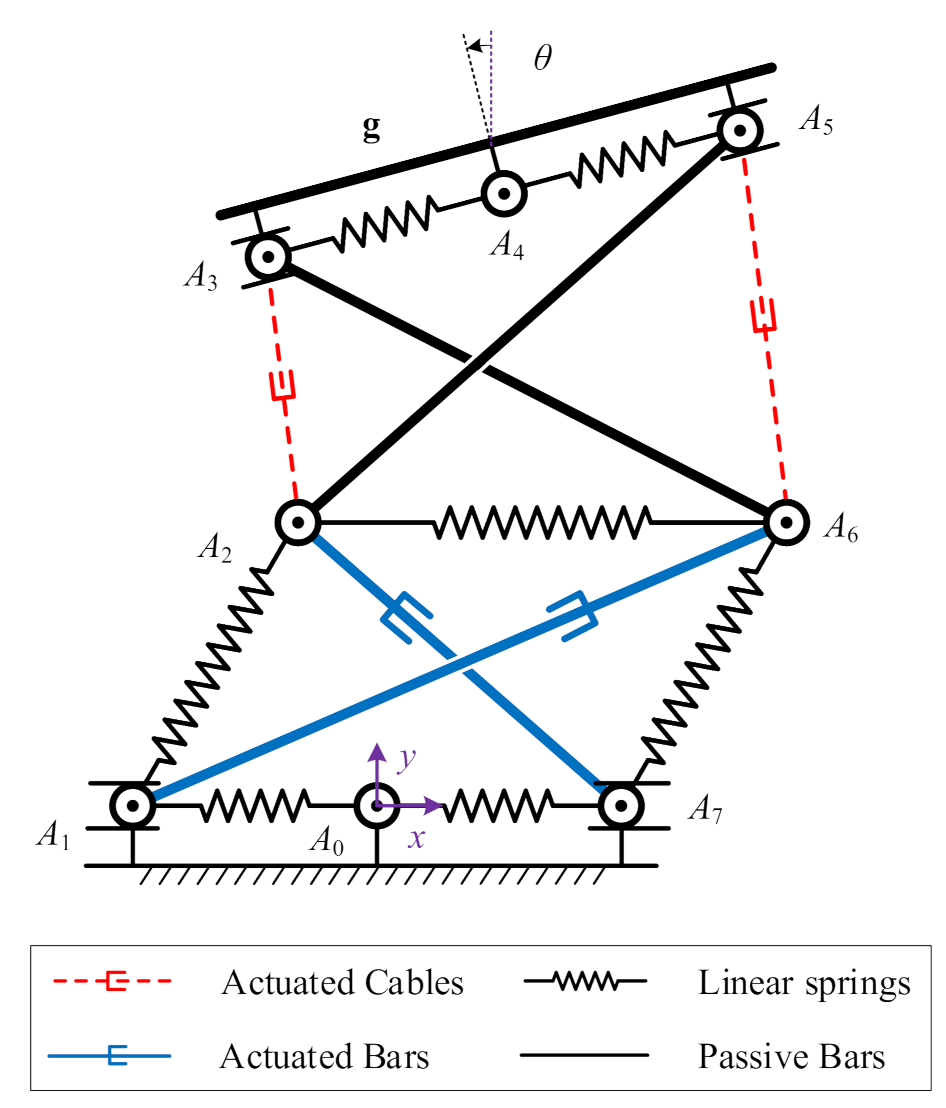
2. Configuration and Actuation Mode

The 3-DOF compliant tensegrity manipulator discussed in this paper is constructed by stacking two SCs, as shown in Figure 1. These two SCs share the member $l_{26}$ for compactness and high stiffness, which is different from the manipulator introduced in Ref. [24]. The proposed mechanism consists of seven passive linear springs, two passive bars, two actuated cables, and two actuated bars. Linear springs are essential tensile elements in TM that provide compliance. The length of passive bars $l_{25}$ and $l_{36}$ are equal to have symmetric structure. Node $A_0$ is fixed at the origin of coordinate system $A_0$-$xy$, and nodes $A_1$ and $A_7$ are connected with the base by prismatic joints. Analogously, end-effector $\mathbf{g}$ is connected to nodes $A_3$, $A_4$, and $A_5$. Cables and bars are generally considered rigid in tensegrity mechanisms to simplify the modeling due to their relatively high axial stiffness compared to the springs. However, in practical implementations where non-metallic material (e.g., plastic) is used to reduce weight, the deformation of cables and bars cannot be ignored. Therefore, the compliance of cables and bars is considered in this work. Besides, all joints are frictionless and the effect of gravity is ignored.

In order to obtain determined planar motion and keep all the springs tensioned, four actuators are used. However, in the inverse kinematics analysis, the end-effector $\mathbf{g}={\left[x_4,y_4,\theta \right]}^{\mathrm{T}}$ only provides three constraining equations, making the mechanism actuation-redundant. Therefore cables $l_{23}$ and $l_{56}$ are designed to actuate synchronously so that the mechanism can have determined motion. The actuation strategy for $l_{23}$ and $l_{56}$ is given as

$$l_{23}+l_{56}=l_{\mathrm{c}},$$

(1)

where $l_{\mathrm{c}}$ is constant. Using the proposed actuation strategy, the forward and inverse kinematics can have smooth motion and stable solution, respectively.

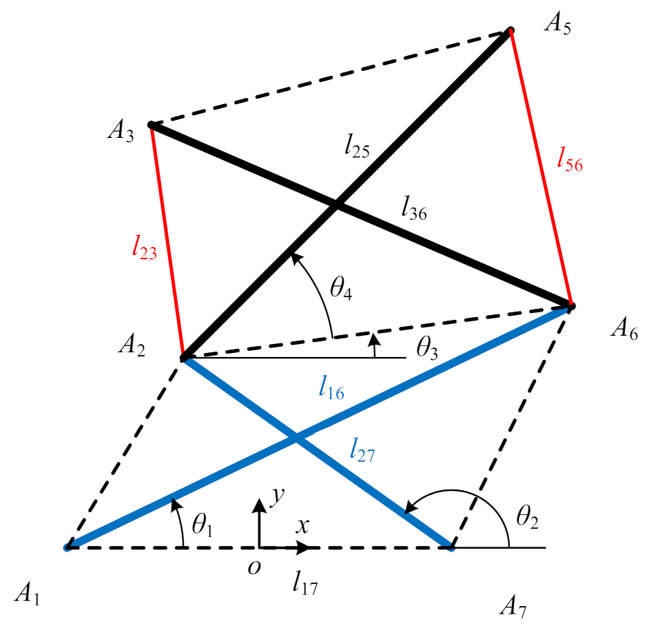
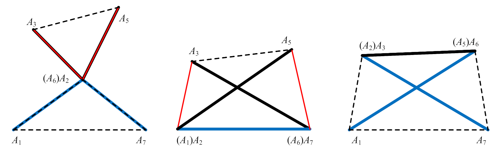
3. Two-Step Kinematics Modeling

3.1. Step-1: Energy-Based Preliminary Modeling

For traditional mechanisms, the number of drives needs to be greater than or equal to the DOFs of the mechanism to ensure the unique motion. However, for the TM with springs, the spring can not be regarded as a constraint. The mechanism maintains equilibrium under springs and can deviate from the equilibrium position under external force. This is also the reason why such mechanisms are compliant. When cables and bars are assumed to be rigid, the mechanism presents three unconstrained DOFs if the actuation variables ${\mathbf{q}}_{\mathrm{a}}={\left[\begin{array}{ccc}{l}_{16}& l_{27}& l_{23}\end{array}\right]}^{\mathrm{T}}$ are given. The generalized coordinates of unconstrained DOFs are selected as ${\mathbf{q}}_{\mathrm{u}}={\left[\begin{array}{ccc}{\theta }_1& {\theta }_2& l_{17}\end{array}\right]}^{\mathrm{T}}$, as shown in Figure 2. Based on geometric conditions, the coordinates of the nodes can be obtained as

$$\begin{array}{c}{A}_1={\left[\begin{array}{c}-l_{17},0\end{array}\right]}^{\mathrm{T}},A_7={\left[\begin{array}{c}{l}_{17},0\end{array}\right]}^{\mathrm{T}}\hfill \\ A_6=A_1+l_{16}{\left[\begin{array}{c}cos{\theta }_1,sin{\theta }_1\end{array}\right]}^{\mathrm{T}}\hfill \\ A_2=A_7+l_{27}{\left[\begin{array}{c}cos{\theta }_2,sin{\theta }_2\end{array}\right]}^{\mathrm{T}}\hfill \end{array}$$

(2)

According to the Cosine theorem in triangles $A_2{A}_5{A}_6$, the angle ${\theta }_4$ can be written as

$${\theta }_4=arccos\left(\frac{{l_{25}}^2+{l_{26}}^2-{\left(l_{\mathrm{c}}-l_{23}\right)}^2}{2l_{25}{l}_{26}}\right)$$

(3)

Then the coordinates of $A_5$ is expressed as

$$A_5=A_2+l_{25}{\left[\begin{array}{cc}cos\left({\theta }_3+{\theta }_4\right)& sin\left({\theta }_3+{\theta }_4\right)\end{array}\right]}^{\mathrm{T}}$$

(4)

with

$${\theta }_3=arccos\frac{\left[x_6-x_2,y_6-y_2\right]{\left[1,0\right]}^{\mathrm{T}}}{\left|{\left(x_6-x_2,y_6-y_2\right)}^{\mathrm{T}}\right|}$$

(5)

In the same way, it is easy to calculate the coordinates of $A_3$.

As the coordinates of all nodes are expressed, the potential energy stored in springs can hence be written as

$$U\left({\mathbf{q}}_{\mathrm{u}},{\mathbf{q}}_{\mathrm{a}}\right)=\frac{1}{2}\sum k_s{\left(l_s-l_{0,s}\right)}^2\left(s=12,17,26,35,67\right)$$

(6)

where $k_{ij}$ is the stiffness of spring $A_i$$A_j$, and $l_{0,ij}$ represents the free-length of the spring. In the energy method, the equilibrium state of the tensegrity mechanism is the minimum potential energy state. Accordingly, it can be obtained by solving the following equations

$$\frac{\partial U\left({\mathbf{q}}_{\mathrm{u}},{\mathbf{q}}_{\mathrm{a}}\right)}{\partial {\mathbf{q}}_{\mathrm{u}}}=\mathbf{0}$$

(7)

Equations (3) and (5) require that $A_2$ and $A_6$ cannot coincide, otherwise, the mechanism will have a singular configuration. In addition, when the two groups of rods are collinear, the second derivative of potential energy is less than 0, which is an unstable equilibrium state, resulting in a singularity of the mechanism too. Without considering the symmetry factor, the typical singular configuration is shown in Figure 3, and the singularity needs to be judged when solving.

3.2. Step-2: FDM Equilibrium Equations

The equilibrium equations of FDM are essentially the equilibrium equations of node forces. This method originates from the form-finding problem of cable-nets and can also be applied to the tensegrity mechanism. There are 8 nodes and 13 members in the proposed mechanism, and a 13 × 8 connectivity matrix $\mathbf{C}$ can describe the topology information of the TM. Supposing that member $m(m=1,2,\dots ,13)$ connects node $A_i$ and node $A_j$$(i,j=0,1,\dots ,7)$. The components of the m-th row of $\mathbf{C}$ are defined as

$$C_{\left(m,p+1\right)}=\left\{\begin{array}{ccc}\begin{array}{c}\mathrm{sign}\left(j-p\right)\\ \mathrm{sign}\left(i-p\right)\\ 0\end{array}& \begin{array}{c}\mathrm{if}p=i\\ \mathrm{if}p=j\\ \mathrm{other}\end{array}& \left(p=0,1,\dots ,7\right)\end{array}\right.$$

(8)

Let $\mathbf{x},\mathbf{y}\in {\mathbf{R}}^8$ denote the vectors of nodal coordinates in x-, y-directions, respectively. The coordinate difference vectors (member vectors) $\mathbf{u},\mathbf{v}\in {\mathbf{R}}^{13}$ expressed in a matrix-vector form as follow

$$\mathbf{u}=\mathbf{Cx},\mathbf{v}=\mathbf{Cy}$$

(9)

Based on $\mathbf{u}$ and $\mathbf{v}$, the lengths of members can be obtained as

$$l_m=\sqrt{u_m^2+v_m^2}\left(m=1,2,\dots ,13\right)$$

(10)

Springs, bars, and cables are assumed to deform linearly. Therefore, given the free length $l_{0,m}$ and axial stiffness $k_m$, the force density of member m can be calculated as

$$q_m=\frac{(l_m-l_{0,m})k_m}{l_m}\left(m=1,2,\dots ,13\right)$$

(11)

Then, the 8 × 8 force density matrix $\mathbf{E}$ is defined as [21]

$$\mathbf{E}={\mathbf{C}}^{\mathrm{T}}\mathbf{QC}$$

(12)

where the diagnosed matrix $\mathbf{Q}$ is expressed as

$$\mathbf{Q}=\mathrm{diag}\left(q_1,q_2,\dots ,q_{13}\right)$$

(13)

If there is no external force acting on the mechanism, the equilibrium equations are

$$\left[\begin{array}{cc}\mathbf{E}(\mathbf{x},\mathbf{y})& \mathbf{0}\\ \mathbf{0}& \mathbf{E}(\mathbf{x},\mathbf{y})\end{array}\right]\left[\begin{array}{c}\mathbf{x}\\ \mathbf{y}\end{array}\right]=\mathbf{0}$$

(14)

Note that $\mathbf{E}$ can be expressed by $\mathbf{x}$ and $\mathbf{y}$. Equation (14) is a set of non-linear equations with respect to nodal coordinates. The geometric constraints considering the fixed constraint and prismatic joints can be written as

$${\Phi }_1={\left[x_0,y_0,y_1,y_7\right]}^{\mathrm{T}}=\mathbf{0}$$

(15)

Meanwhile, in order to avoid the mirrored configuration, the coordinate range should be constrained by

$${\Phi }_2={\left[-x_1,x_7,y_2,y_6,y_3-y_2,y_5-y_6\right]}^{\mathrm{T}}>\mathbf{0}$$

(16)

3.3. Kinematics Solving Procedure

As the dimension of ${\mathbf{q}}_{\mathbf{a}}$ and the end-effector $\mathbf{g}$ are all three, there is only one unique stable solution within a reasonable range after excluding symmetrical results. According to the two-step method, both forward and inverse kinematics require solving nonlinear equations twice, as shown in Figure 4. Iterative methods, such as the Levenberg-Marquardt algorithm, are suitable for solving these equations.

4. Performance Criteria

4.1. Stability

Eigenvalues of the stiffness matrix can indicate the stability of a tensegrity mechanism. Denoting $\mathbf{X}={[{\mathbf{x}}^{\mathrm{T}},{\mathbf{y}}^{\mathrm{T}}]}^{\mathrm{T}}$ as the generalized coordinates vector and the 16 × 16 global stiffness matrix $\mathbf{K}$ can be computed as [21]

$$\mathbf{K}=\left[\begin{array}{c}{\mathbf{C}}^{\mathrm{T}}{\mathbf{UL}}^{-\mathbf{1}}\\ {\mathbf{C}}^{\mathrm{T}}{\mathbf{VL}}^{-\mathbf{1}}\end{array}\right]\overline{\mathbf{K}}{\left[\begin{array}{c}{\mathbf{C}}^{\mathrm{T}}{\mathbf{UL}}^{-\mathbf{1}}\\ {\mathbf{C}}^{\mathrm{T}}{\mathbf{VL}}^{-\mathbf{1}}\end{array}\right]}^{\mathrm{T}}+{\mathbf{I}}_2\otimes \mathbf{E}$$

(17)

with

$$\begin{array}{c}\mathbf{L}=\mathrm{diag}(l_1,l_2,\dots ,l_{13})\hfill \\ \overline{\mathbf{K}}=\mathrm{diag}(k_1,k_2,\dots k_{13}){\mathbf{L}}^{-1}\hfill \\ \mathbf{U}=\mathrm{diag}\left(\mathbf{u}\right)\hfill \\ \mathbf{V}=\mathrm{diag}\left(\mathbf{v}\right)\hfill \end{array}$$

(18)

where ${\mathbf{I}}_2$ is a 2 × 2 identity matrix and ⊗ denotes the tensor product. This formulation considers the stressed equilibrium state as the reference state. The stiffness matrix in Equation (17) is a global matrix with respect to all coordinates. Removing rows and columns related to fixed coordinates ($x_0$, $y_0$, $y_1$, and $y_7$), the 12 × 12 stiffness matrix ${\mathbf{K}}_1$ of all moveable nodal coordinates can be obtained. Let $\lambda ={[{\lambda }_1,{\lambda }_2,\dots ,{\lambda }_{12}]}^{\mathrm{T}}$ denote the eigenvalues of ${\mathbf{K}}_1$, and the TM is considered stable when all the eigenvalues are positive, as

$$\mathrm{Stable}\iff \lambda >\mathbf{0}$$

(19)

Stability is the basic characteristic of tensegrity. If there are non-positive eigenvalues, it indicates that there is singularity caused by the collinearity of members.

4.2. End-Effector Workspace

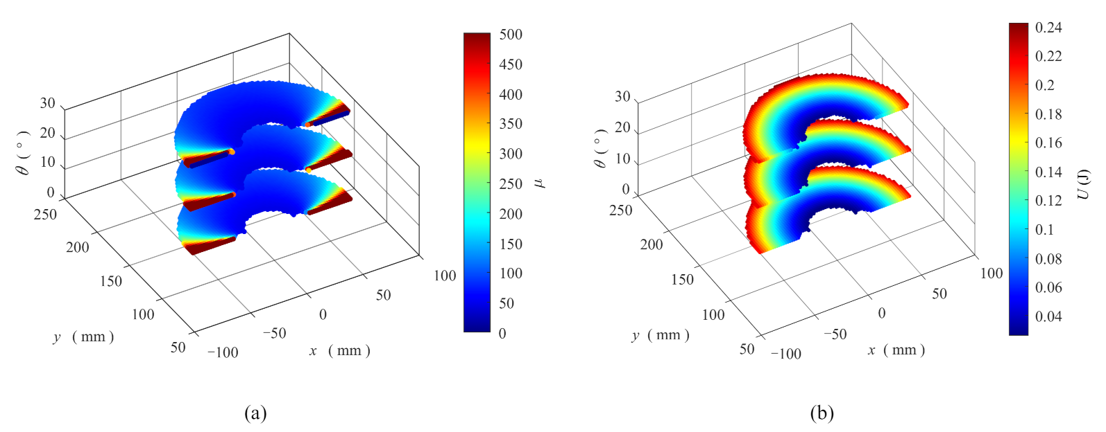
Except for the limitation of the actuators, spring length is another factor that limits the workspace of the end-effector. The springs need to be elongated to ensure that the TM is tensioned and the length cannot exceed the elastic elongation limitation. At present, the conventional method of obtaining the workspace is discretizing ${\mathbf{q}}_{\mathbf{a}}$ or $\mathbf{g}$ and then solving the kinematics equations. The workspace of the end-effector considering geometric constraints, stability, and spring lengths, is defined as

$$\mathbf{W}=\left\{\mathbf{g}\left({\mathbf{q}}_{\mathrm{a}}\right)\mid \begin{array}{c}\left[\begin{array}{cc}\mathbf{E}& \mathbf{0}\\ \mathbf{0}& \mathbf{E}\end{array}\right]\left[\begin{array}{c}\mathbf{x}\\ \mathbf{y}\end{array}\right]=\mathbf{0}\hfill \\ {\Phi }_1\left(\mathbf{x},\mathbf{y}\right)=\mathbf{0}\hfill \\ {\Phi }_2\left(\mathbf{x},\mathbf{y}\right)>\mathbf{0}\hfill \\ \lambda \left({\mathbf{q}}_{\mathrm{a}},\mathbf{x},\mathbf{y}\right)>\mathbf{0}\hfill \\ {\mathbf{L}}_{\mathrm{S}}\left({\mathbf{q}}_{\mathrm{a}},\mathbf{x},\mathbf{y}\right)\in \left[{\mathbf{L}}_{\mathrm{S}}^{\mathrm{low}},{\mathbf{L}}_{\mathrm{S}}^{\mathrm{up}}\right]\hfill \end{array}\right\}$$

(20)

where ${\Phi }_1$ and ${\Phi }_2$ are geometric constraints, $\lambda$ denote the eigenvalues of the stiffness matrix ${\mathbf{K}}_1$, and ${\mathbf{L}}_{\mathrm{S}}$ denotes the lengths of springs constrained within $\left[{\mathbf{L}}_{\mathrm{S}}^{\mathrm{low}},{\mathbf{L}}_{\mathrm{S}}^{\mathrm{up}}\right]$. Cable stress, failure, and buckling of bars are not considered here.

4.3. Manipulability

The 3 × 3 kinematic Jacobian matrix maps the relationship between the actuation velocities and the end-effector velocities, which is a valuable means to evaluate the manipulability. It can also be used to determine whether there are singularity states.

$$\dot{\mathbf{g}}=\mathbf{J}{\dot{\mathbf{q}}}_{\mathrm{a}}$$

(21)

The centered finite differences method is used to compute J, and the manipulability measure is expressed as

$$\mu =\sqrt{det\left({\mathbf{JJ}}^{\mathrm{T}}\right)}$$

(22)

4.4. Potential Energy and Stiffness of End-Effector

Generally, a high level of potential energy is expected to resist deformation when relatively large external loads are applied. However, a low level of potential energy suggests that the manipulator is more mobile and safer in specific situations, e.g., using it as a surgical tool. In practical applications, the proportional adjustment of spring stiffness can directly change the potential energy.

In order to quantify the stiffness intuitively, the translational stiffness (normal stiffness, tangential stiffness) and rotational stiffness of the end-effector can be calculated based on the stiffness matrix. The tangential stiffness of the end-effector can be obtained by applying unit force along the tangential direction ($l_{45}$) on node $A_4$, solving the node displacements using ${\mathbf{K}}_1$, and calculating stiffness. The calculation of normal and rotational stiffness is similar to that of tangential stiffness.

5. Optimization under Workspace Constraint

5.1. Optimization Model

For a designated task workspace, it is not easy to determine the installation location and design member lengths. In some situations, we need to design the TM as compact as possible. Therefore, we develop an optimization method to achieve the most compact design of the mechanism under workspace constraints.

The optimization model is defined as

$$\begin{array}{c}\mathrm{find}:{\mathbf{x}}_{\mathrm{D}}=[x_0,y_0,l_{\mathrm{p}},l_{\mathrm{c}},l_{\mathrm{s}},l_{\mathrm{a}}^{\mathrm{low}},l_{\mathrm{a}}^{\mathrm{up}}]\hfill \\ \min :F_{\mathrm{obj}}=2l_{\mathrm{p}}+l_{\mathrm{c}}+5l_{\mathrm{s}}+l_{\mathrm{a}}^{\mathrm{low}}+l_{\mathrm{a}}^{\mathrm{up}}\hfill \\ \mathrm{s}.\mathrm{t}.:\begin{array}{c}{\mathbf{W}}^{\mathrm{t}}\subset \mathbf{W}\left({\mathbf{x}}_{\mathrm{D}}\right)\hfill \\ \mu \ne 0\hfill \end{array}\hfill \end{array}$$

(23)

where [$x_0$, $y_0$] is the installation location of $A_0$, $l_{\mathrm{p}}$ is the free-length of two passive bars, $l_{\mathrm{c}}$ is the sum length of cables, $l_s$ is the free-length of springs ($l_{12}$, $l_{17}$, $l_{26}$, $l_{35}$, and $l_{67}$), $\left[l_{\mathrm{a}}^{\mathrm{low}},l_{\mathrm{a}}^{\mathrm{up}}\right]$ are the limitation of actuated bars, ${\mathbf{W}}^{\mathrm{t}}$ is the task workspace, which is determined by the actual requirements of the end-effector, $\mathbf{W}\left({\mathbf{x}}_{\mathrm{D}}\right)$ is the workspace defined by Equation (20). $l_{23}$ change in [0.2 $l_{\mathrm{c}}$, 0.8 $l_{\mathrm{c}}$]. The potential energy and stiffness can be changed without affecting the workspace by changing the spring stiffness in equal proportion. Therefore, they are not considered in the optimized model.

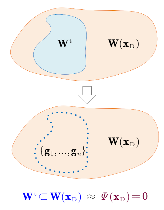
5.2. Constraint Simplification

The above problem is a seven-dimensional single-objective constrained optimization problem. As the objective function is simple, the core of this problem is how to transform complex workspace constraints (set constraints) into relatively simple numerical constraints. Using the discretization method to calculate the workspace defined Equation (20) is time-consuming and unnecessary in the optimization process.

For the TM in this paper, its workspace is a three-dimensional simply connected space. Based on this, as long as the outer contour of the task workspace ${\mathbf{W}}_{\mathrm{B}}^{\mathrm{t}}$ is enclosed by $\mathbf{W}\left({\mathbf{x}}_{\mathrm{D}}\right)$, it is safe to say that the entire task workspace is a subset of $\mathbf{W}\left({\mathbf{x}}_{\mathrm{D}}\right)$, as

$${\mathbf{W}}^{\mathrm{t}}\subset \mathbf{W}\left({\mathbf{x}}_{\mathrm{D}}\right)\iff {\mathbf{W}}_{\mathrm{B}}^{\mathrm{t}}\subset \mathbf{W}\left({\mathbf{x}}_{\mathrm{D}}\right)$$

(24)

Then, we discretize the contour ${\mathbf{W}}_{\mathrm{B}}^{\mathrm{t}}$ to obtain finite poses and reduce the computational cost.

$$\left\{{\mathbf{g}}_1,{\mathbf{g}}_2,\dots ,{\mathbf{g}}_n\right\}\in {\mathbf{W}}_{\mathrm{B}}^{\mathrm{t}}$$

(25)

Therefore, the constraint function can be defined as

$$\Psi \left({\mathbf{x}}_{\mathrm{D}}\right)=\sum _{i=1}^{n}f\left({\mathbf{g}}_i\right)$$

(26)

with

$$f\left({\mathbf{g}}_i\right)=\left\{\begin{array}{cc}1& {\mathbf{g}}_i\notin \mathbf{W}\left({\mathbf{x}}_{\mathrm{D}}\right)\\ 0& {\mathbf{g}}_i\in \mathbf{W}\left({\mathbf{x}}_{\mathrm{D}}\right)\end{array}\right.$$

(27)

In this way, the workspace constraint is expressed by a numerical constraint function, as illustrated in Figure 5. It is noteworthy that the number of discrete poses on the task workspace contour may influence constraint modeling accuracy. The fewer discrete poses we use, the faster the optimization algorithm runs, but it has the risk that the designed TM cannot reach all the poses, especially for a target workspace of irregular shape.

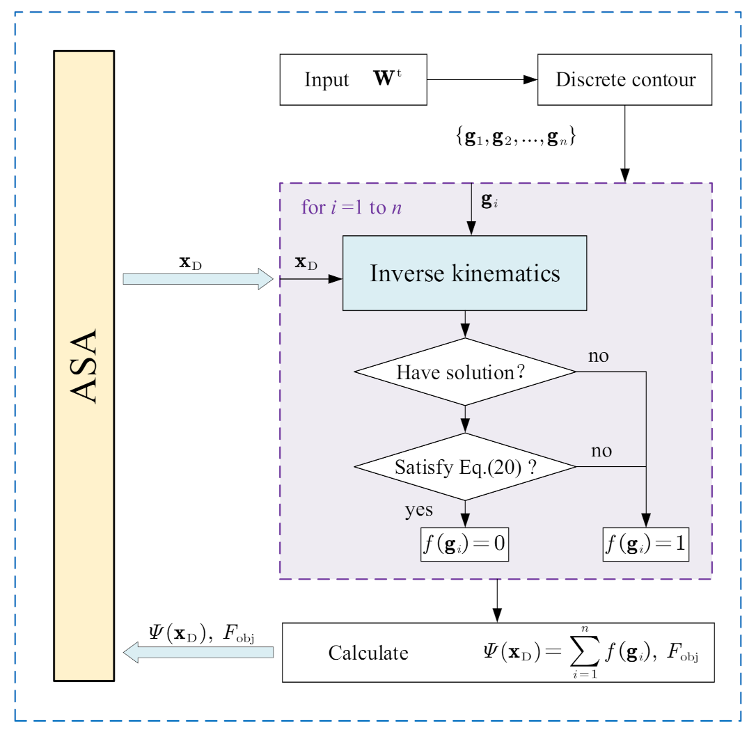
5.3. Optimization Procedure

As shown in Figure 6, after the task workspace is determined, the contour is extracted and discretized to get n poses. The constraint function and objective function value under given design variables can be obtained by solving n sets inverse kinematics equations. Considering that the constraint function of this problem is not expressed analytically, gradient-based optimization algorithms are not suitable, and these methods rely too much on initial values. This paper uses the adaptive simulated annealing (ASA), a global optimization algorithm, to solve this problem.

6. Results and Discussion

6.1. Workspace Analysis

In this section, we use a numerical example to analyze the workspace form. Two passive bars of the 3-DOF TM are set to 100 mm, and the length of the actuating bars varies in the interval [40, 160] mm. The sum length of two cables ($l_{23}$ + $l_{56}$) is set equal to 140 mm. All bars and cables have the same axial stiffness of 1.0$\times {10}^2$ N/mm. Three different springs are used in the tensegrity mechanism, as presented in

Table 1. Free length and axial stiffness of springs.

Springs	Free Length (mm)	Stiffness (N/mm)	$\left[{\mathit{l}}_{}^{\mathbf{low}},{\mathit{l}}_{}^{\mathbf{up}}\right]$ (mm)
$l_{12}$, $l_{67}$	20	0.05	[40,120]
$l_{01}$, $l_{07}$, $l_{34}$, $l_{45}$	10	0.1	[20,60]
$l_{26}$	20	0.1	[40,120]

. In order to better visualize the workspace boundary, we slice the workspace with respect to rotation angle $\theta$, as shown in Figure 7.

As shown in Figure 7a, x, y, and $\theta$ components of the end-effector pose are constrained in the intervals of [−102, 102] mm, [90, 206] mm, and [−64, 64]${}^{\circ }$, respectively. Except for $\pm {60}^{\circ }$, the translational mobility at the other $\theta$ is similar. Meanwhile, the workspace boundary shifts a little bit along the x-axis with different $\theta$. For example, as illustrated in Figure 7c,d, when $\theta =0^{\circ }$, the workspace is symmetrical with respect to the line x = 0 mm, and when $\theta ={30}^{\circ }$, the workspace is symmetrical about the line x = −17 mm. The original intention of the design is to use the cable-actuated SC($A_2{A}_3{A}_5{A}_6$) to produce angular ($\theta$) and the bar-actuated SC($A_1{A}_2{A}_6{A}_7$) to produce displacement(x, y). However, the results show that there is a coupling between the two SCs. When the cable-actuated SC generates a specific $\theta$, there is an x-direction displacement, which is the main reason for the offset.

The manipulability measure $\mu$ is distributed in the range [13.6, 26.9] with a mean value of 19.8, and there is no singularity in the whole workspace. On the whole, the distribution of $\mu$ has two trends. The first is that with the increase of $\left|\theta \right|$, $\mu$ has a downward trend, significantly when $\theta =\pm {60}^{\circ }$, $\mu$ drops to near 14. The second trend is that under the same $\theta$, the farther $\mathbf{g}$ is away from the origin, the larger $\mu$ is, as shown in Figure 7c.

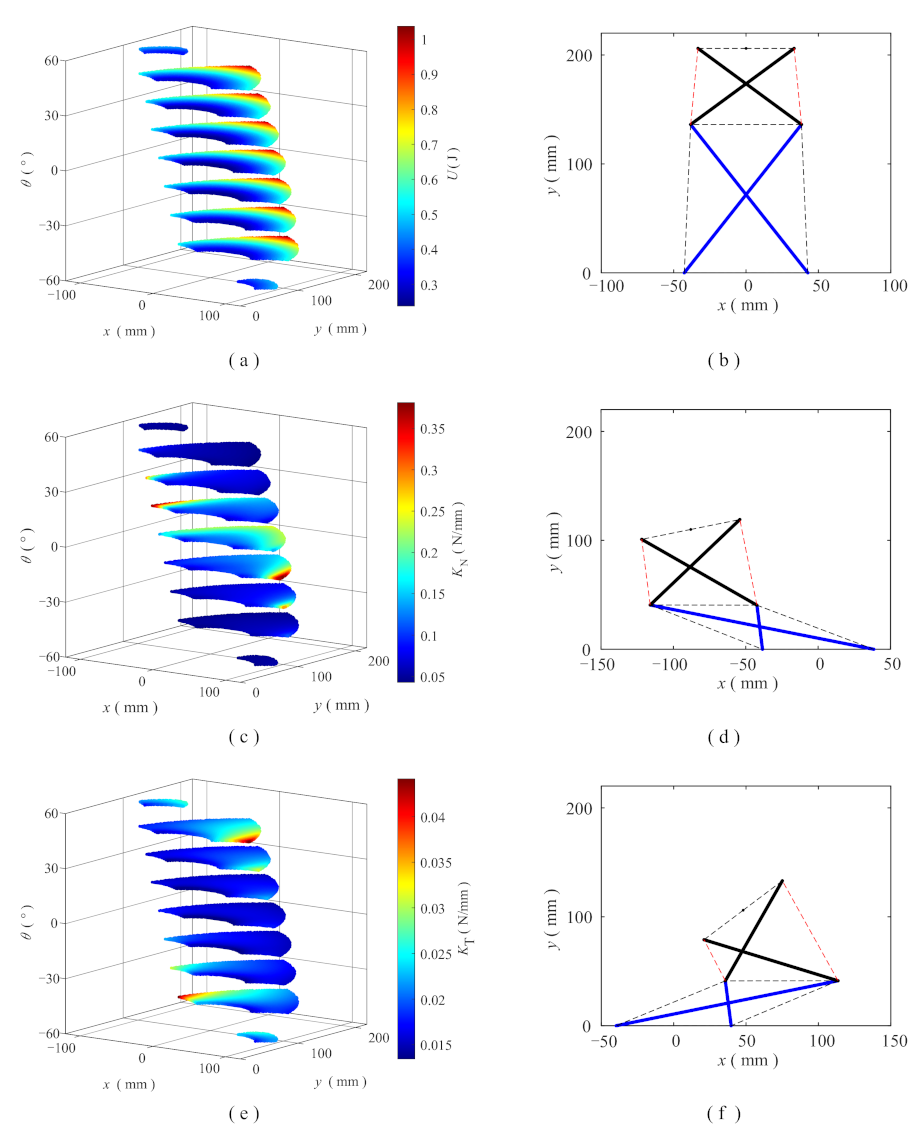
6.2. Potential Energy and Stiffness of End-Effector

As shown in Figure 8a, the maximum and minimum potential energy are 1.0373 J and 0.2378 J, respectively, suggesting that the proposed TM requires at most 0.7995 J actuating energy to move even if there is no external load. At different $\theta$, the potential energy distribution is similar, and it is mainly affected by the translation of the end-effector. As expected, when the actuated bars are both at the maximum length and $l_{23}=0.5l_c$, the TM own maximum potential energy, as shown in Figure 8b.

Figure 8c shows that the distribution of normal stiffness is in [0.0429, 0.3812] N/mm, and the mean value is 0.1050 N/mm. In particular, the normal stiffness increases significantly near $\mathbf{g}={\left[82,126,-5\right]}^{\mathrm{T}}$ and $\mathbf{g}={\left[-82,126,15\right]}^{\mathrm{T}}$, which may be related to the approach between the orientation of actuated bars and the normal direction of end-effector. Take $\mathbf{g}={\left[-82,126,15\right]}^{\mathrm{T}}$ as an example, its configuration is shown in Figure 8d. The tangential stiffness varies in [0.0134, 0.0441] N/mm, and its mean value is 0.0193 N/mm, as shown in Figure 8e. These results show that the tangential stiffness is significantly lower than the normal stiffness. One reason for this phenomenon is that the connections at $A_0$ and $A_4$ are equivalent to a series connection springs. The unevenness of stiffness in different directions is a drawback of this mechanism, and excessive tangential force must be avoided during application.

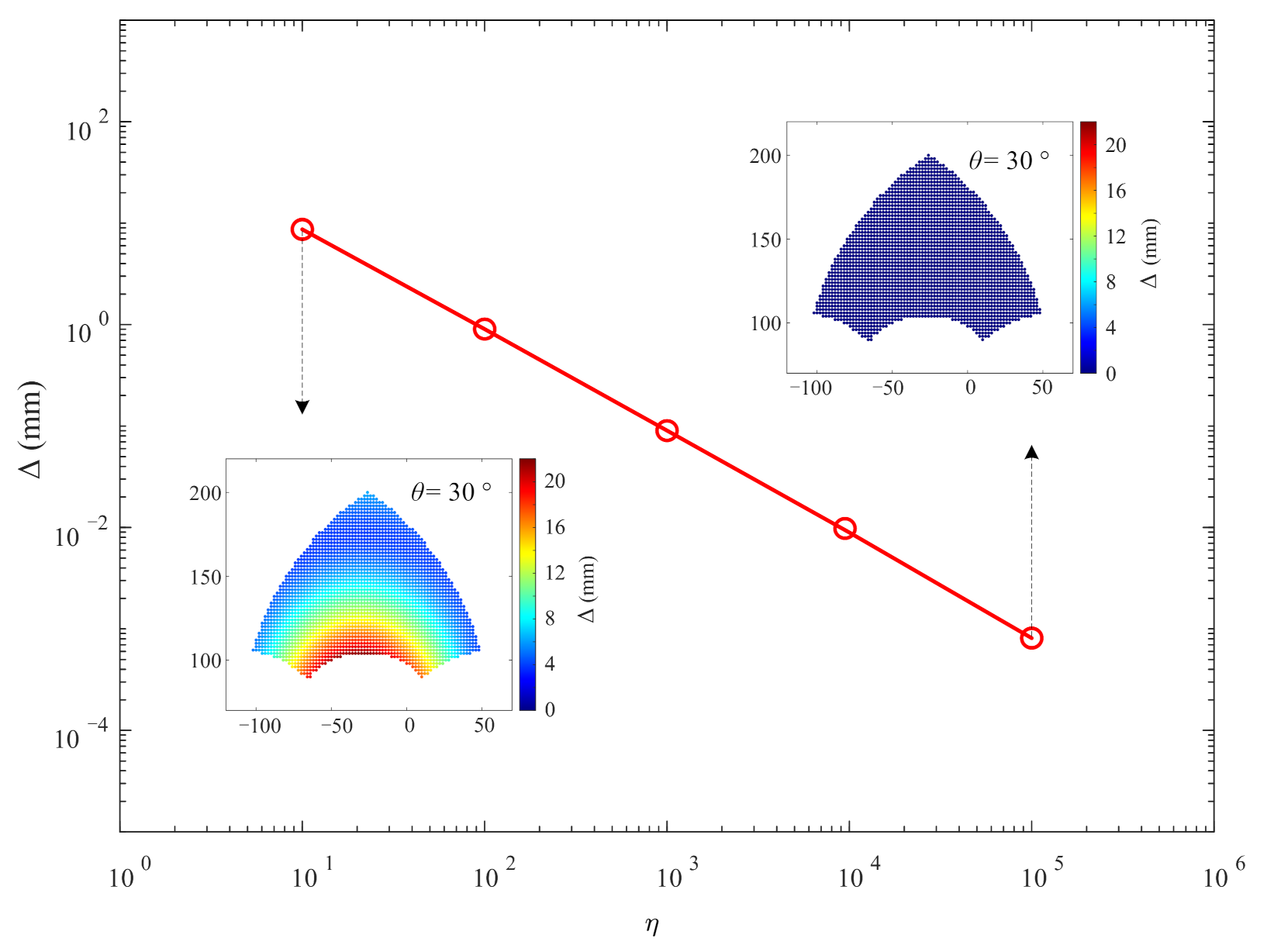
6.3. Effect of the Flexibility of Bars and Cables on Kinematics

By calculating the inverse kinematics under different bar/cable stiffness, we can understand the influence of bar/cable flexibility on kinematics and further evaluate the necessity of the proposed two-step method. The mechanism configuration, size, and springs are consistent with Section 6.1, and all bars and cables have the same axial stiffness. We can define the stiffness ratio as

$$\eta =\frac{k^{\mathrm{bar}\_\mathrm{cable}}}{k^{\mathrm{spring}}}.$$

(28)

The effects of the flexibility of bars/cables can be quantitatively expressed as

$$\Delta \left(\eta ,\mathbf{g}\right)=\left|{\mathbf{q}}_{\mathrm{a}}^{\mathrm{flex}}\left(\eta ,\mathbf{g}\right)-{\mathbf{q}}_{\mathrm{a}}^{\mathrm{rigid}}\left(\mathbf{g}\right)\right|,$$

(29)

where ${\mathbf{q}}_{\mathrm{a}}^{\mathrm{flex}}$ is inverse kinematics solution of the two-step method, ${\mathbf{q}}_{\mathrm{a}}^{\mathrm{rigid}}$ is the inverse kinematics solution assuming bars and cables are rigid.

When $\theta ={30}^{\circ }$, the mean values of $\Delta$ are shown in Figure 9. As expected, the larger the stiffness ratio of the bar to the spring, the smaller difference of the ${\mathbf{q}}_{\mathrm{a}}$ between the rigid and flexible models. The relationship between $\Delta$ and $\eta$ is close to linear in logarithmic coordinate. When $\eta$ = 10, the average $\Delta$ is 8.687 mm, and when $\eta$ = ${10}^5$, the value falls into 8.132 $\times {10}^{-4}$. Meanwhile, the distribution of $\Delta$ is also related to $\mathbf{g}$. Take $\eta$ = 10 and $\theta ={30}^{\circ }$ as an example. The maximum $\Delta$ is 21.462 mm at $\mathbf{g}={\left[-26,104,30\right]}^{\mathrm{T}}$ and minimum $\Delta$ is 4.044 mm at $\mathbf{g}={\left[-26,200,30\right]}^{\mathrm{T}}$. Based on the comparison results, if the ratio of the bar stiffness and spring stiffness is less than ${10}^2$, the flexibility of the bars and cables have a relatively noticeable effect on the kinematics. It is necessary to use FDM for accurate modeling. When the stiffness ratio is more than ${10}^5$, it will not produce an obvious error if the bars/cables are assumed rigid.

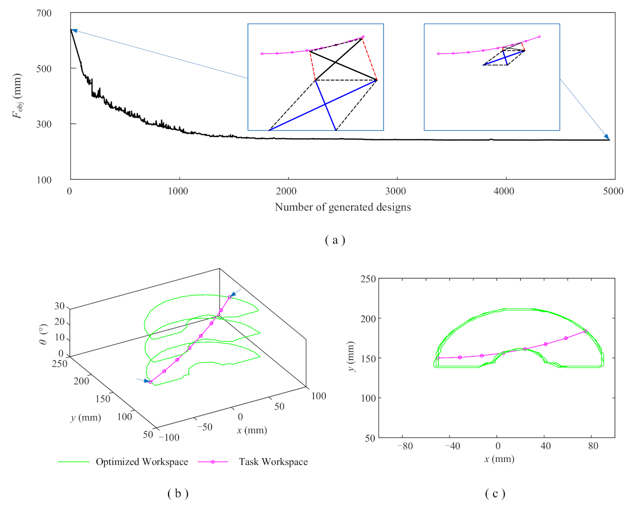
6.4. Optimization Examples

Two examples are used here to validate the proposed optimization method, and the initial design is presented in Section 6.1 with $F_{\mathrm{obj}}$ = 640 mm.

The first example is to design a TM that can rotate around a fixed point, and this remote-center-rotation constraint is modeled as

$${\mathbf{W}}_1^{\mathrm{t}}=\left\{\mathbf{g}={[x_4,y_4,\theta ]}^{\mathrm{T}}\left|\begin{array}{c}{x}_4=250cos\theta -50\hfill \\ y_4=250sin\theta +400\hfill \\ \theta \in [0,\frac{\pi }{6}]\hfill \end{array}\right.\right\}$$

(30)

This remote-center-rotation manipulator is usually used in medical applications [25,26]. In this situation, the task workspace is a smooth curve, and we have ${\mathbf{W}}_{\mathrm{B}}^{\mathrm{t}}$ = ${\mathbf{W}}^{\mathrm{t}}$. Using the proposed contour sampling method in Section 5.2, we use eight sample poses evenly distributed on the ask workspace to model the constraint.

After generating 4947 designs by ASA, the objective $F_{\mathrm{obj}}$ declined by 62.3%, from 640 mm to 241.3 mm, as shown in Figure 10a. The optimized workspace($\theta \in {[0,30]}^{\circ }$) and task workspace are displayed in Figure 10b,c. Two endpoints of the curve almost fall on the contour of the optimized workspace, which means that a relatively optimal design has been found. Figure 11 are manipulability and potential energy plots of the optimized configuration. Compared with the initial configuration, the maximum manipulability increased significantly, but mainly concentrated in the edge region. The potential energy distribution is very similar to the initial design. At the same time, the decline of the overall potential energy level indicates that the elastic potential energy stored by the mechanism itself will also decrease after the overall size is reduced.

Another example is to design a TM with workspace expressed as

$${\mathbf{W}}_2^{\mathrm{t}}=\left\{\mathbf{g}={[x_4,y_4,\theta ]}^{\mathrm{T}}\left|\begin{array}{c}\frac{{x_4}^2}{{40}^2}+\frac{{\left(y_4-150\right)}^2}{{20}^2}⩽1\hfill \\ \theta \in [-\frac{\pi }{9},\frac{\pi }{9}]\hfill \end{array}\right.\right\}$$

(31)

The workspace is an elliptical cylinder region in shape. Analogously, 48 poses on the contour are used to model the constraint. After generating 4997 designs by ASA, the objective $F_{\mathrm{obj}}$ declined by 69.4 %, from 640 mm to 195.7 mm, as shown in Figure 12a. As shown in Figure 12b,c, the workspace contour of the designed TM and the task workspace contour are almost tangent at $\mathbf{g}={\left[-36,159,-20\right]}^{\mathrm{T}}$, $\mathbf{g}={\left[36,159,20\right]}^{\mathrm{T}}$, and $\mathbf{g}={\left[0,129,\dots \right]}^{\mathrm{T}}$. The above two examples obtain the optimal installation positions and sizes of the TMs under respective workspace constraints, suggesting that the proposed method is effective.

7. Conclusions

This paper introduces a 3-DOF planar tensegrity manipulator with a compact structure constructed by two SCs. An advanced two-step kinematic modeling method is proposed to analyze its kinematics characteristics. The first step of this method is to estimate the equilibrium state of TM using the energy method, assuming that the bars and cables are rigid. Then, considering the flexibility of bars and cables, the second step is to obtain the accurate pose by solving the FDM equations using the state of the previous step as the initial design of iteration. After that, a sampling-based optimization method under workspace constraint is proposed. In this method, we use discrete points on the contour of a given target workspace to model constraints numerically. The following conclusions are obtained:

• The numerical example suggests that the TM has a relatively sizeable 3-DOF workspace and no singularity under the constraints of driving variables and spring elongation limitation;
• The stiffness of the end-effector in the tangential direction is significantly less than that in the normal direction, and excessive tangential force must be avoided during application;
• The flexibility of the bars and cables have a relatively noticeable effect on the kinematics when the bars-to-spring stiffness ratio is less than ${10}^3$, and it is necessary to use the two-step method for accurate modeling. When the ratio is more extensive than ${10}^5$, flexibility can be ignored.
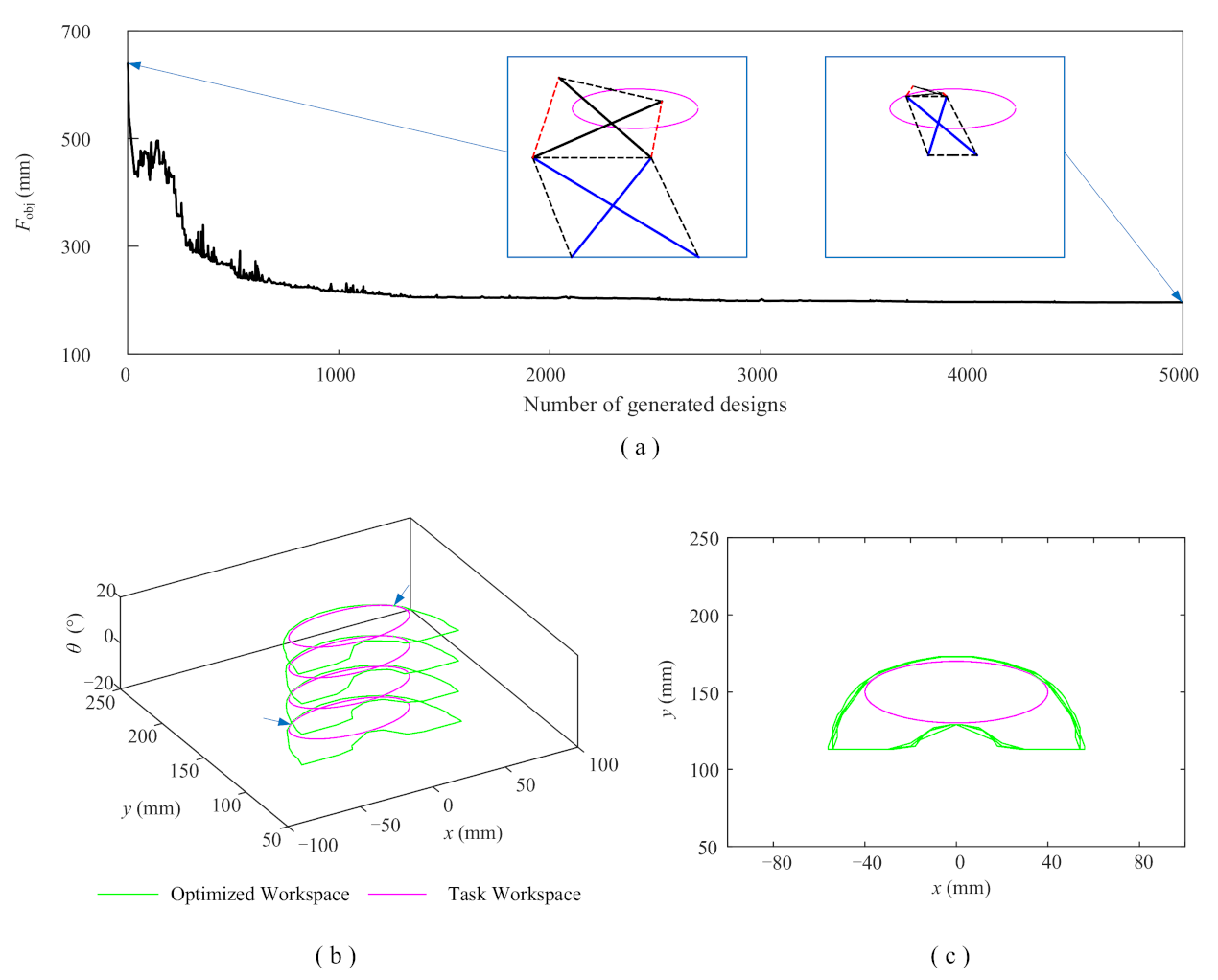
• Two study cases are used to validate the effectiveness of the optimization method. After optimization, the objectives are reduced by 62.3% and 69.4% , respectively. Moreover, the target poses are located on and tangent to the contour of the workspace, suggesting that optimal designs considering compactness are obtained.

References

1. Richard, B.F. Tensile-Integrity Structures. U.S. Patent 3063521, 13 November 1962. [Google Scholar]
2. Castro, G.; Levy, M.P. Analysis of the georgia dome cable roof. In Proceedings of the Computing in Civil Engineering and Geographic Information Systems Symposium, Dallas, TX, USA, 7–9 June 1992; pp. 566–573. [Google Scholar]
3. Zhan, W.D.; Dong, S.L. Advances in cable domes. J. Zhejiang Univ. (Eng. Sci.) 2004, 38, 1298–1307. [Google Scholar]
4. Zavodszky, M.I.; Ming, L.; Thorpe, M.F.; Day, A.R.; Kuhn, L.A. Modeling correlated main-chain motions in proteins for flexible molecular recognition. Proteins-Struct. Funct. Bioinform. 2010, 57, 243–261. [Google Scholar] [CrossRef]
5. Luo, Y.; Xu, X.; Lele, T.; Kumar, S.; Ingber, D.E. A multi-modular tensegrity model of an actin stress fiber. J. Biomech. 2008, 41, 2379–2387. [Google Scholar] [CrossRef] [Green Version]
6. Scarr, G. A consideration of the elbow as a tensegrity structure. Int. J. Osteopath. Med. 2012, 15, 53–65. [Google Scholar] [CrossRef]
7. Sultan, C. Tensegrity deployment using infinitesimal mechanisms. Int. J. Solids Struct. 2014, 51, 21–22. [Google Scholar] [CrossRef] [Green Version]
8. Sychterz, A.; Smith, I. Damage mitigation of near-full-scale deployable tensegrity structure through behavior biomimetics. J. Struct. Eng. 2020, 146, 04019181. [Google Scholar] [CrossRef]
9. Yıldız, K.; Lesieutre, G. Deployment of n-strut cylindrical tensegrity booms. J. Struct. Eng. 2020, 146, 04020247. [Google Scholar] [CrossRef]
10. Rahmat Abadi, B.; Farid, M.; Mahzoon, M. Introducing and analyzing a novel three-degree-of-freedom spatial tensegrity mechanism. J. Comput. Nonlinear Dyn. 2014, 9, 94. [Google Scholar]
11. Rovira, A.; Mirats-Tur, J. Control and simulation of a tensegrity-based mobile robot. Robot. Auton. Syst. 2009, 57, 526–535. [Google Scholar] [CrossRef]
12. Caluwaerts, K.; Despraz, J.; Iscen, A.; Sabelhaus, A.P.; Bruce, J.; Schrauwen, B.; SunSpiral, V. Design and control of compliant tensegrity robots through simulation and hardware validation. J. R. Soc. Interface 2014, 11, 20140520. [Google Scholar] [CrossRef] [Green Version]
13. Du, W.; Ma, S.; Li, B.; Wang, M.; Hirai, S. Force analytic method for rolling gaits of tensegrity robots. IEEE/ASME Trans. Mechatron. 2016, 21, 2249–2259. [Google Scholar] [CrossRef]
14. Luo, A.; Liu, H. Analysis for feasibility of the method for bars driving the ball tensegrity robot. J. Mech. Robot. 2017, 9, 051010. [Google Scholar] [CrossRef]
15. Furet, M.; Wenger, P. Workspace and Cuspidality Analysis of a 2-X Planar Manipulator. In Mechanism Design for Robotics; Springer International Publishing: Cham, Switzerland, 2019; pp. 110–117. [Google Scholar]
16. Arsenault, M.; Gosselin, C. Kinematic, static and dynamic analysis of a planar 2-dof tensegrity mechanism. Mech. Mach. Theory 2006, 41, 1072–1089. [Google Scholar] [CrossRef]
17. Boehler, Q.; Vedrines, M.; Abdelaziz, S.; Poignet, P.; Renaud, P. Influence of Spring Characteristics on the Behavior of Tensegrity Mechanisms. In ARK: Advances in Robot Kinematics; Springer International Publishing: Cham, Switzerland, 2014; pp. 161–169. [Google Scholar]
18. Boehler, Q.; Charpentier, I.; Vedrines, M.S.; Renaud, P. Definition and computation of tensegrity mechanism workspace. J. Mech. Robot. 2015, 7, 044502. [Google Scholar] [CrossRef]
19. Wenger, P.; Chablat, D. Kinetostatic analysis and solution classification of a class of planar tensegrity mechanisms. Robotica 2019, 37, 1214–1224. [Google Scholar] [CrossRef] [Green Version]
20. Rahmat Abadi, B.; Shekarforoush, S.; Mahzoon, M.; Farid, M. Kinematic, stiffness, and dynamic analyses of a compliant tensegrity mechanism. J. Mech. Robot. 2014, 6, 041001. [Google Scholar] [CrossRef]
21. Zhang, J.Y.; Ohsaki, M. Tensegrity Structures; Springer: Tokyo, Japan, 2015. [Google Scholar]
22. Moored, K.W.; Kemp, T.H.; Houle, N.E.; Bart-Smith, H. Analytical predictions, optimization, and design of a tensegrity-based artificial pectoral fin. Int. J. Solids Struct. 2011, 48, 3142–3159. [Google Scholar] [CrossRef] [Green Version]
23. Begey, J.; Vedrines, M.; Andreff, N.; Renaud, P. Selection of actuation mode for tensegrity mechanisms: The case study of the actuated snelson cross. Mech. Mach. Theory 2020, 152, 103881. [Google Scholar] [CrossRef]
24. Begey, J.; Vedrines, M.; Renaud, P. Design of tensegrity-based manipulators: Comparison of two approaches to respect a remote center of motion constraint. IEEE Robot. Autom. Lett. 2020, 5, 1788–1795. [Google Scholar] [CrossRef]
25. Zorn, L.; Renaud, P.; Bayle, B.; Goffin, L.; Lebosse, C.; de Mathelin, M.; Foucher, J. Design and evaluation of a robotic system for transcranial magnetic stimulation. IEEE Trans. Biomed. Eng. 2012, 59, 805–815. [Google Scholar] [CrossRef] [PubMed]
26. Bruyas, A.; Geiskopf, F.; Renaud, P. Toward unibody robotic structures with integrated functions using multimaterial additive manufacturing: Case study of an mri-compatible interventional device. In Proceedings of the IEEE/RSJ International Conference on Intelligent Robots and Systems, Hamburg, Germany, 28 September–2 October 2015; pp. 1744–1750. [Google Scholar]
Figure 1. Configuration of the 3-DOF manipulator.
Machines 09 00256 g001
Figure 2. Actuation variables and generalized coordinates.
Machines 09 00256 g002
Figure 3. Typical singular configuration.
Machines 09 00256 g003
Figure 4. Kinematics solving procedure.
Machines 09 00256 g004
Figure 5. Schematic diagram of constraint simplification.
Machines 09 00256 g005
Figure 6. Optimization procedure.
Machines 09 00256 g006
Figure 7. Workspace and manipulability.(a) Isometric view. (b) θ = 60 . (c) θ = 0 . (d) θ = 30 .
Machines 09 00256 g007
Figure 8. Potential energy and stiffness of end-effector. (a) Potential energy. (b) Maximum potential energy state. (c) Normal stiffness of end-effector. (d) Maximum normal stiffness state. (e) Tangential stiffness of end-effector. (f) Maximum tangential stiffness state.
Machines 09 00256 g008
Figure 9. Effect of flexibility.
Machines 09 00256 g009
Figure 10. Workspace of the optimized configuration and task workspace (Example 1). (a) Optimization history, (b) isometric view, (c) top view.
Machines 09 00256 g010
Figure 11. Manipulability and potential energy of optimized configuration (Example 1). (a) Manipulability, (b) potential energy.
Machines 09 00256 g011
Figure 12. Workspace of the optimized configuration and task workspace (Example 2). (a) Optimization history. (b) Isometric view. (c) Top view.
Machines 09 00256 g012