Bearing Remaining Useful Life Prediction Based on a Scaled Health Indicator and a LSTM Model with Attention Mechanism

Abstract

Rotor systems are of considerable importance in most modern industrial machinery, and the evaluation of the working conditions and longevity of their core component—the rolling bearing—has gained considerable research interest. In this study, a scale-normalized bearing health indicator based on the improved phase space warping (PSW) and hidden Markov model regression was established. This indicator was then used as the input for the encoder–decoder LSTM neural network with an attention mechanism to predict the rolling bearing RUL. Experiments show that compared with traditional health indicators such as kurtosis and root mean square (RMS), this scale-normalized bearing health indicator directly indicates the actual damage degree of the bearing, thereby enabling the LSTM model to predict RUL of the bearing more accurately.

1. Introduction

Bearing reliability evaluation and remaining useful life (RUL) prediction have received extensive attention due to the increasingly extreme working conditions of the entire system [1,2]. Generally, bearing life follows a specific statistical distribution that can be inferred from a large number of life data samples. However, due to the influence of assembly errors, material defects, and load fluctuations, in practice, bearing life has strong randomness. Studies carried out using public bearing life datasets can be taken as examples. In the accelerated degradation datasets of bearings collected by FEMTO-ST on the PRONOSTIA experimental platform, the RUL of the test bearing under specific load and speed conditions falls within the range of 2–7 h [3]. The results of the datasets provided by the BPC system from Sumyoung Technology Co. are similar, where the life spans of the test bearings are between 30 min and 8 hours [4]. In addition to the accelerated degradation experiments mentioned above, the RULs obtained from the natural degradation experiments are also different. For example, in the life test of the Rexnord ZA-2115 double-row bearing carried out on the durability test rig by NASA, the results are between seven days and one month [5]. Therefore, it is highly challenging to predict bearing RUL from a statistical point of view accurately. For this reason, in engineering practice, research focus has shifted to the study of the RUL of individual bearing, considering its actual working condition. Kundu [6] predicted the bearing RUL by establishing a Weibull proportional regression model based on the monitored signals of the PRONOSTIA platform. By combining the respective advantages of long- and short-term memory (LSTM) and statistical process analysis, Liu [7] proposed a new network to predict the bearing RUL using the datasets released by NASA and FEMTO-ST. Huang [8] introduced the transfer learning method and constructed a transfer depth-wise separable convolution recurrent network to predict the bearing RUL from the same public datasets considering different work conditions.

Various mathematical and physical models were successfully applied to the prediction of bearing RUL. However, an overview of the aforementioned studies indicates that the actual degree of damage to the test bearing was not considered in the studies using the public bearing datasets; only the physical signals, e.g., acceleration and temperature signals, monitored in the bearing life test were studied. Take the FEMTO dataset as an example, and it did not provide damage sizes of the test bearings. The termination criterion was only created by the acceleration signal exceeding the threshold. Similarly, the same criterion was defined as the end of bearing life in many other representative studies [7,8,9,10]. However, it was found in our experiments that under the same operating conditions, even if the same acceleration threshold is used as the test termination condition, the final damage degree, namely the crack length in the spall area, can be remarkably different. 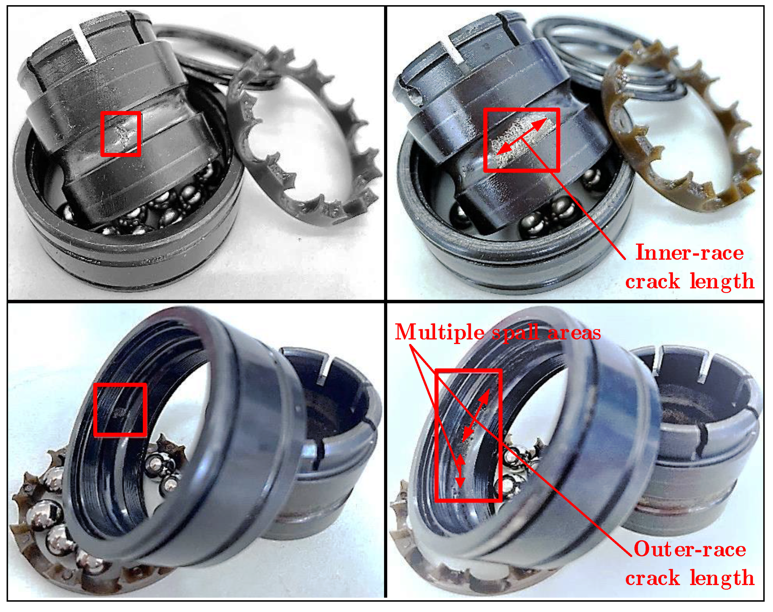Figure 1 shows the damage to four test bearings under the same operating condition, for which the tests were stopped based on the same acceleration threshold. It was demonstrated that even bearings with the same damage exhibited utterly different degrees of damage under similar acceleration levels. Therefore, under different application scenarios, the construction of health indicators and the development of life prediction methods need to be explicitly designed.

Among the conventional health indicators [11,12], the root mean square (RMS) is the most commonly used, although it has the disadvantage of strong fluctuations. Additionally, the relative root mean square (RRMS) was adopted in the literature to reduce the negative impact of the fluctuations on the calculation results [9]. In addition to the RMS, Zhong [13] used a nonparametric health index for machine condition monitoring by combining envelope spectrum and statistic model, and principal component analysis (PCA) was used by Kundu [6] for dimensionality reduction of feature vectors to extract those features with better monotonicity. Xu [14] purposed a new health indicator called moving average cross-correlation of the power spectral density (MACPSD) to predict the health state of ball bearing. However, the problem with these health indicators in practice is that their calculated values are not directly related to the actual damage degree of the bearing, as shown by the crack length of the spall area in Figure 1.

In RUL prediction, researchers have proposed numerous prediction methods, which can be mainly divided into the model-driven method, data-driven method, and hybrid method. Model-driven methods, such as the Paris-Erdogan method [15], can accurately predict the bearing RUL under different working conditions. Still, the accuracy depends on establishing a practical model based on the physical system. The data-driven method utilizes statistical models or artificial intelligence (AI) models to predict the RUL, where the statistical model is often referred to as an empirical model-based method. For example, Kumar [16] combined the Kullback–Leibler divergence and Gaussian process regression to predict the RUL. Li [11] and Qiu [17] presented a stochastic process to predict the RUL. Xing [18] and Li [19] proposed a mixed Gauss model–hidden Markov model (GM-HMM) to predict the RUL of wind turbine bearings. Other methods include AI mathematical models such as the support vector machine [9] and artificial neural network [20], which can handle complex systems problems without any prior knowledge. However, data-driven methods can only manage the targeted work condition and exhibit no universal adaptability. On the other hand, the hybrid method combines the advantages of the model-driven method and the data-driven method; techniques such as the Kalman filter [21] and particle filter [22] belong to this type. Although many works were proposed to study the problem of bearing RUL prediction, few relevant studies have considered detecting accurate damage occurrence time and end of lifetime, which are crucial for prediction outputs. Antoni [23] used entropic evidence to detect the initial faults in rotating machinery. Chegini [24] purposed ensemble empirical model decomposition and wavelet packet decomposition to detect the initial faults in rotating machinery, and the Nirwan [25] used the acoustic emission to detect faults. Although such mentioned works provided relatively accurate detection results, the detection models or the extracted features originated from extensive calculations. It is not easy to implement such methods under the requirement of real-time response, mainly when the prediction of bearing RUL is an ongoing process.

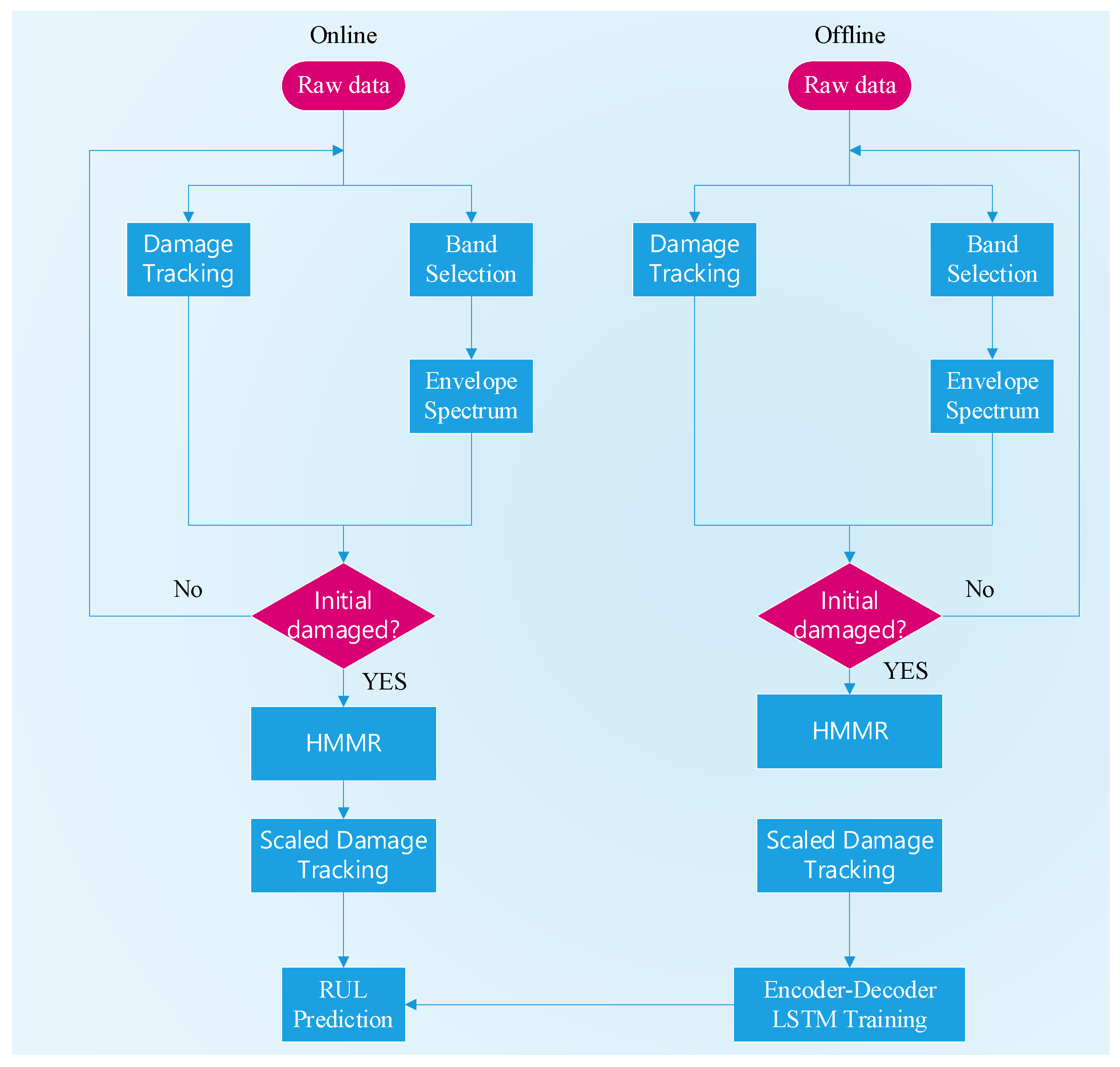
To address the problem of detecting initial bearing damage, an adaptive envelope analysis method was employed in Section 2. Subsequently, in Section 3, an improved phase-space warping (PSW) algorithm was proposed to construct the bearing health indicator, followed by the indicator normalization using the hidden Markov model regression (HMMR) introduced in Section 4. The test bearing datasets verified the capability of the normalized health indicator to reasonably reflect the actual degree of bearing damage. In Section 5, the health indicator threshold, indicating the true damage extent, was defined as the end of bearing lifetime, which allows the proposed encoder-decoder long-short term memory (LSTM) model with an attention mechanism to predict the bearing RUL. The results through analyzing the experimental data of bearing life proved the effectiveness of the proposed method, see Section 6.

2. Detection of Bearing Initial Damage

In engineering practice, it is not practical to take the operation starting time of the rolling bearing as the initiation for bearing RUL prediction. This method has the shortcomings of extensive computation and unclear engineering significance. In contrast, predicting the bearing RUL after detecting the initial damage through real-time monitoring of signals can help determine the maintenance schedule and have more practical engineering significance as the amount of calculation is relatively small. Therefore, before predicting the bearing RUL, it is necessary to develop a damage detection algorithm with high sensitivity and strong robustness to determine the starting time of prediction (i.e., damage occurrence time). This paper proposed a sensitive and stable envelope analysis method that does not need a large amount of calculation and can adaptively determine a reasonable envelope bandwidth to identify the initial damage of the bearing as well as the starting time for RUL prediction.

2.1. Adaptive Frequency Band Selection

The vibration signal should theoretically contain ball passing frequencies (BPFs) when bearing damage occurs, whose calculation formulas are shown as follows, in which, the ω_R, D_P, b_P, α and $n$ are, respectively, the rotational speed, pitch diameter, roller diameter, contact angle and number of rollers.

$$\mathrm{BSF}=\frac{1}{2D_{\mathrm{b}}}{D}_{\mathrm{p}}\left[1-{\left(\frac{D_{\mathrm{b}}}{D_{\mathrm{p}}}\cos \alpha \right)}^2\right]$$

(1)

$$\mathrm{FTF}=\frac{1}{2}{\omega }_{\mathrm{R}}\left(1-\frac{D_{\mathrm{b}}}{D_{\mathrm{P}}}\cos \alpha \right)$$

(2)

$$\mathrm{BPFI}=\frac{1}{2}{\omega }_{\mathrm{R}}n\left(1+\frac{D_{\mathrm{b}}}{D_{\mathrm{P}}}\cos \alpha \right)$$

(3)

$$\mathrm{BPFO}=\frac{1}{2}{\omega }_{\mathrm{R}}n\left(1-\frac{D_{\mathrm{b}}}{D_{\mathrm{P}}}\cos \alpha \right)$$

(4)

Envelope analysis is the standard procedure to extract the ball passing frequencies, called the damage-related characteristic frequencies, from the signal envelopes in real applications. In the envelope analysis, the selection of frequency band for the bandpass filter is a critical step, for which researchers have proposed various methods. Among them, the fast Kurtogram [26] is the most commonly used one for selecting envelope frequency bands. The signal components extracted by this method are primarily impulsive, as fast Kurtogram was initially designed to be highly sensitive to the impacts hidden in the original signal. Due to the impulsive nature of bearing damage response, the method has proven effective in many applications. However, in some other cases, the slide-roll ratio of the bearing or the collision between the cage and rolling elements under normal operations also have significant impacts. As a result, envelope analysis based on fast Kurtogram would lead to misjudgment owing to its excessive sensitivity. Recently, Peeters [27] proposed to select the optimal frequency band based on the sparsity of envelope signals. This approach utilizes the second-order stationarity of healthy bearing signals to maximize the envelope sparsity, thereby realizing the selection of the envelope frequency band. However, when the normal impacts break the hypothesis of second-order cyclostationary, this method would still fail to extract the characteristic frequencies. Therefore, we shift our focus to develop a sensitive and robust detection method for damage frequency extraction. The method must predict the bearing RUL automatically and avoid the interferences caused by slight impacts from the slide-roll mechanism or the collision between the cage and rolling elements during the regular operation of the bearing.

It is well-known that the bearing damage-induced impacts excite vibrations at the bearing resonance frequency [28]. In other words, if the resonance frequency can be identified, the frequency band close to it can be used as the filter band to perform the envelope analysis. To this end, the peaks of power spectral densities (PSDs) of bearing accelerations are used as the center frequencies of the envelope frequency bands. Moreover, it is assumed that the natural frequency rests at the local peak of its PSDs under 10 kHz [29]. Then, eleven frequency bands from the local minimum were selected as the envelope passbands to extract the characteristic frequencies of the bearing damage, see Figure 2.

2.2. Initial Damage Detection

Spectral peaks of a healthy bearing would be evident at the corresponding characteristic frequencies in the envelope spectrum.

Specifically, when a local spalling occurs in the inner-ring, the ball passing frequency of the inner-ring (BPFI), its low-order harmonics, and the nearby sidebands may all exhibit peak characteristics. When a bearing has an outer-ring spalling, the ball passing frequency of the outer-ring (BPFO) and its low-order harmonics would also exhibit corresponding peak characteristics.

Table 1. Geometrical parameters and the characteristic frequencies of the test bearing.

Parameters	Value	Parameters	Value
Inner race diameter Di	25.4 mm	Static load ratings	7828.87 N
Outer race diameter Do	52.0 mm	Dynamic load ratings	14,011.9 N
Pitch diameter DP	38.7 mm	Contact angle	$0°$
Roller diameter Db	7.92 mm
Number of rollers n	9
Rotation speed ${\omega }_{\mathrm{R}}$	33 Hz
BPFI	178 Hz	BPFO	118 Hz
BSF	77 Hz	FTF	13 Hz

shows the geometrical parameters, experimental conditions and the calculated characteristic frequencies of our test bearing.

On the other side, Figure 3 and Figure 4 show the envelope spectrums of the inner- and outer-ring damaged bearing, respectively. They are obtained from the pre-divided bandpass frequency bank with eleven passbands, see Figure 2 as an example.

Each time the acceleration signal is collected from the accelerometer, we select filter bands from the envelope spectrum using the method described in Section 2.1. Then, the obtained amplitudes of the characteristic frequencies would be compared with the pre-defined threshold to determine whether damage has occurred in the bearing. In this paper, the threshold is defined as ${\sigma }_{\mathrm{th}}=3{\sigma }_{\mathrm{n}}$, where ${\sigma }_{\mathrm{n}}$ represents noise level expressed as local average, excluding the amplitudes of BPFs. Taking the definition of the BPFO threshold as example, the BPFO can be determined using Equation (5). In the equation, $f_s$ represents the bandwidth that needs to be captured, $F_s(\mathrm{freq})$ represents the amplitude at the target frequency, $n_s$ is the number of spectral lines, and the BPFO is the ball passing frequency of the outer-ring damaged bearing.

$$\begin{array}{l}{\sigma }_n=\frac{1}{n_s-1}\left[{\displaystyle \sum _{\mathrm{freq}=f_{s1}}^{\mathrm{freq}=f_{s2}}{F}_s(\mathrm{freq})}-F_s(\mathrm{BPFO})\right]\\ f_{s1}=\mathrm{BPFO}-f_s\\ f_{s2}=\mathrm{BPFO}+f_s\end{array}$$

(5)

To avoid misjudgment, when the initial damage occurs in the bearing, it is assumed that at least two of the amplitudes at its characteristic frequencies, i.e., the BPF, the low-order harmonics, and the sideband frequencies (if inner-ring damage occurs in the bearing), would exceed the threshold [30]. Therefore, 11 time instants can be determined based on the 11 envelope spectrums as the bearing service time goes by. The minimum of these time instants is defined as the occurrence time of bearing damage.

Figure 5a,b are the zoom-in envelope spectrums corresponding to the damage occurrence time obtained by the above method. Compared with other frequency components, the characteristic frequencies are dominant in amplitude (see the BPFI and its sideband in Figure 5a and the BPFO in Figure 5b). Thus, when damages occur to the bearing, if reasonable bandpass filter ranges are selected, there would be significant increases in the amplitudes of characteristic frequencies in the envelope spectrum. On the other side, Figure 5c,d show the envelope spectrums for the same time instant obtained after selecting the filter band using the fast Kurtogram. The amplitudes of the BPFI and its sideband in Figure 5c, together with the amplitude of BPFO in Figure 5d, are not significantly larger than those of other frequency components. Disappointingly, the fast Kurtogram based envelope analysis method fails to detect bearing damages at last and cannot be applied to initialize the prediction of bearing RUL.

3. Construction of Health Indicator

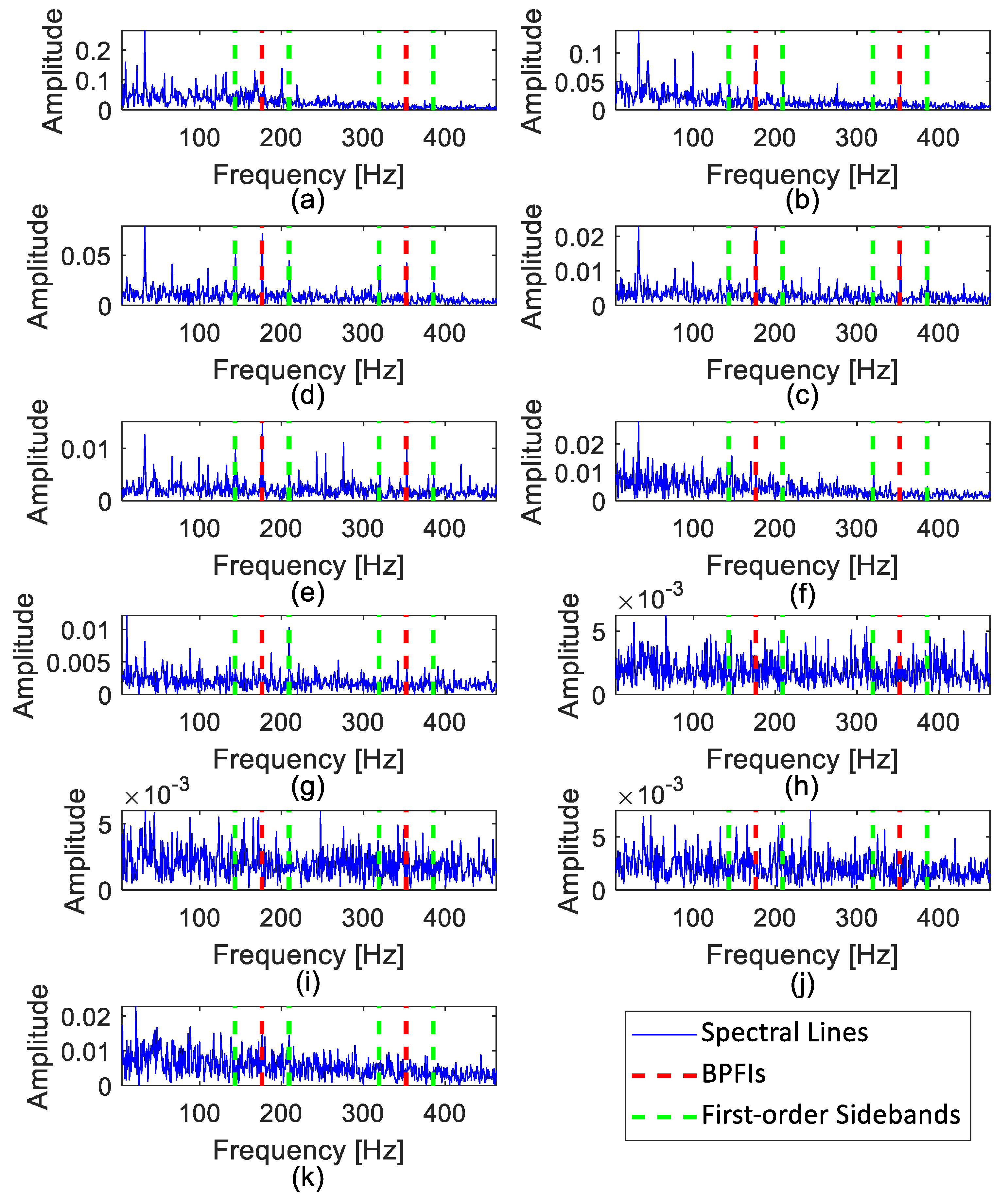
The amplitudes of BPFs in the envelope spectrum can help determine the occurrence time of bearing initial damage. Nevertheless, it is not a good option as a health indicator to predict the RUL because of its poor monotonicity against the bearing degradation process. Therefore, once the initial damage is detected, a new bearing health indicator needs to be established to predict the bearing RUL.

Previous studies often use time-domain statistical features, e.g., RMS, kurtosis, and peak-to-peak value, as health indicators in industrial applications. In contrast, applicational cases related to frequency-domain features, e.g., wavelet transform and Hilbert-Huang Transform, were presented in the references until recent years. However, due to the introduction of pre-defined parameters in the mathematical transformation, its applications in industrial fields still have limitations. Time-domain features are still the most commonly used health indicators. The calculation formulas of RMS and kurtosis are as follows:

$$\begin{array}{l}{F}_{\mathrm{RMS}}=\sqrt{\frac{1}{n}{\displaystyle \sum _{i=1}^n{\left|x_i\right|}^2}}\\ F_{\mathrm{KURT}}=\frac{1}{n}{\displaystyle \sum _{i=1}^n\frac{{\left(x_i-{\mu }_x\right)}^4}{{\sigma }_x^4}}\end{array}$$

(6)

where x_i is the raw data and n is the number of data points used to calculate the feature value. μ_x and σ_x are respectively the mean value and standard deviation of the raw data.

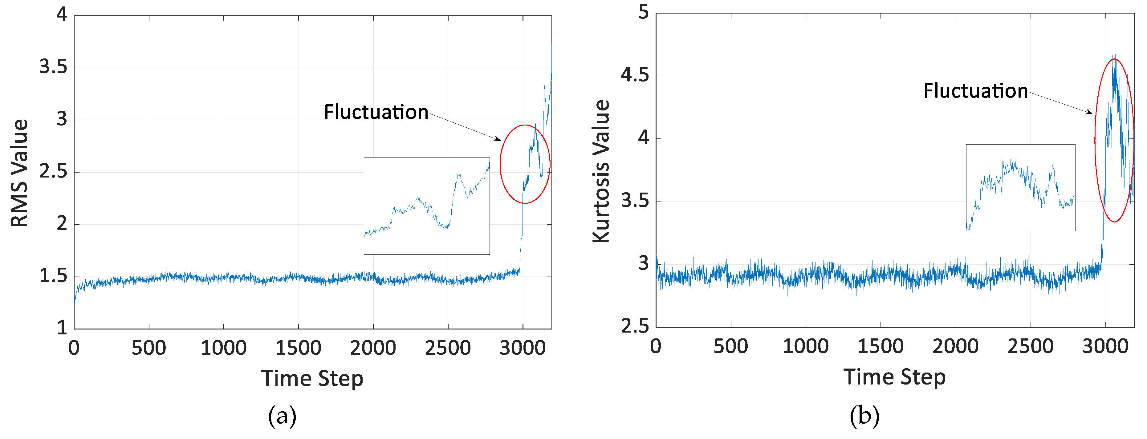
However, owing to the complexity of actual physical systems, it is challenging to accurately express the service status of the bearing with the above features. Their respective trends in Figure 6 shows statistical characteristics such as RMS and kurtosis. The RMS exhibits evident fluctuations, while the kurtosis would decrease as the number of defect-induced impacts increases when the bearing damage becomes more severe. These poor monotonic features are likely to cause misjudgment of bearing life in engineering applications. Furthermore, for features extracted based on AI methods, it is challenging to explain the physical meaning of such features. Most importantly, the above-mentioned features are incapable of reflecting the crack length of the bearing spall area shown in Figure 1. As shown by a group of experimental results listed in

Table 2. Comparisons of the Scaled PSW, RMS and Kurtosis for different crack length.

	Bearing 1-1	Bearing 1-2	Bearing 1-3	Bearing 1-4	Bearing 1-5
Crack Length	3.5 mm	2 mm + 1 mm	3 mm	2.5 mm + 0.5 mm	3 mm + 0.5 mm
Scaled PSW	2.687	1.845	2.049	1.733	2.607
RMS	2.582	3.307	2.893	3.286	2.781
Kurtosis	1.553	1.947	2.014	1.313	1.334

, when the experiment ended, the RMS and kurtosis after scale standardization (the standardization method is introduced in Section 4) cannot effectively reflect the crack length in the bearing (+represents multiple spall areas, as shown by Figure 1). Therefore, to overcome the afore-described challenges, this paper proposes to use the PSW algorithm as the feature extraction method.

3.1. Phase Space Warping (PSW) Theory

PSW is an effective method for evaluating the damage of multi-layer dynamical systems, which was first proposed by Chelidze [31]. From the perspective of dynamic theory, the damage evolution of the entire rotor system can be regarded as a high-order system composed of a “fast time” scale and a “slow time” scale. Its definition is as follows:

$$\begin{array}{l}\dot{x}=f\left[x,\mu \left(\varphi \right),t\right]\\ \dot{\varphi }=\epsilon g\left(x,\varphi ,t\right)\end{array}$$

(7)

In Equation (7), $x\in R^n$ is the “fast time” scale variable, which can be measured directly. $\varphi \in R^m$ is the “slow time” scale variable, which can directly reflect the damage state of the entire system but cannot be measured directly. $f(\cdot )$ and $g(\cdot )$ are the “fast time” and “slow time” scaling functions, respectively. $\mu (\cdot )$ is a function of the variable $\varphi$, t represents time, and $\epsilon (0<\epsilon \ll 1)$ is a constant parameter that defines the damage rate of the system. The response states of the bearing system at the initial time point t₀ and after operating for a certain period t_p can be expressed as

$$\begin{array}{l}{x}_0=F\left[x_0,\mu \left({\varphi }_0\right),t_0\right]\\ x_t=F\left[x_p,\mu \left({\varphi }_{\mathrm{t}}\right),t_p\right]\end{array}$$

(8)

Suppose that the bearing system always maintains its initial state without experiencing any change or damage, then the response of the bearing system can be calculated using Equation (9).

$$x_R\left(t_p\right)=F\left[x_p,\mu \left({\varphi }_0\right),t_p\right]$$

(9)

Therefore, with the initial operating state of the bearing system as the reference state, there is $t_0=t_R$. Then, the damage state of the bearing system (or damage tracking) can be expressed as follows:

$$e=F\left[x_p,\mu \left({\varphi }_P\right),t_p\right]-F\left[x_p,\mu \left({\varphi }_R\right),t_p\right]$$

(10)

In Ref. [31], after performing the Taylor expansion, the bearing system’s damage state can be finally expressed as

$$e=\frac{\partial F}{\partial \mu }\frac{\partial \mu }{\partial {\varphi }_p}\left({\varphi }_p-{\varphi }_R\right)+O\left({\Vert {\varphi }_p-{\varphi }_R\Vert }^2\right)+O\left(\epsilon \right)$$

(11)

where $O(\cdot )$ represents higher-order infinitesimal. In this paper, the raw acceleration signal of the bearing is regarded as an observable “fast time” scale variable, while the damage state of the bearing system is regarded as a “slow time” scale variable.

Typically, to calculate the damage state of the bearing, the phase space reconstruction theory based on the Takens embedding theorem would be introduced, and the damage state of the bearing would be quantified on this basis. The phase space reconstruction is mathematically expressed as follows:

$$y_R\left(n\right)={\left[x_R\left(n\right),x_R\left(n+\tau \right),\dots ,x_R\left(n+\left(D-1\right)\tau \right)\right]}^{\mathrm{T}}n=1,\dots ,N\left(D-1\right)\tau$$

(12)

where $y_R\in R^D$ is the reference initial state of the phase space of the bearing system, n is the number of vectors in the phase space, and N is the total number of observation data points. $\tau$ and D represent the time delay and embedding dimension of the phase space, which can be calculated using the mutual information [32] method and Cao’s method [33]. Theoretically, the unknown mapping between the reconstruction vector $y_R(n)$ in the reference phase space and that of the next step $y_R(n+1)$ on the “slow time” scale—that is, under the reference state of the bearing ${\varphi }_R$—can be expressed as

$$y_R(n+1)=P^{\tau }\left[y_R\left(n\right);{\varphi }_R\right]$$

(13)

In engineering, linear regression is the most straightforward and generic model for establishing the mapping between reconstruction vectors $\{y_R(n)\}$ and $\{y_R(n+1)\}$ in the reference phase space, as shown by Equation (14).

$$y_R\left(n+1\right)=A_n\stackrel{⌢}{y}\left(n\right)$$

(14)

where $A_n\in R^{d\times (d+1)}$ is the model parameter, and $\stackrel{⌢}{y}\left(n\right)\in R^{d+1}$ is the combination of the input phase space and the identity matrix

$$\stackrel{⌢}{y}\left(n\right)={\left[y_{{}_R}^{\mathrm{T}}\left(n\right),1\right]}^{\mathrm{T}}$$

(15)

Based on the simple linear regression model, the parameter matrix A_n can be calculated as follows:

$$\begin{array}{l}{A}_n=Y_{n+1}{\left({\stackrel{⌢}{Y}}_n\right)}^{\mathrm{T}}{\left[{\stackrel{⌢}{Y}}_n{\left({\stackrel{⌢}{Y}}_n\right)}^{\mathrm{T}}\right]}^{-1}\\ {\stackrel{⌢}{Y}}_n=\left[{\stackrel{⌢}{y}}^1\left(n\right){\stackrel{⌢}{y}}^2\left(n\right)\dots {\stackrel{⌢}{y}}^I\left(n\right)\right]\end{array}$$

(16)

where $Y_n\in R^{d\times I}$ is the vector combination of the I nearest neighbors of the reconstruction vector y_n in the reference phase space, and ${\stackrel{⌢}{Y}}_n\in R^{(d+1)\times q}$. Y_n+1 is the target response, that is, the combination of the next step vectors of the I nearest neighbor vectors. However, in actual scenarios, the “slow time” scale parameter (i.e., the operating state of the bearing) is in a state of continuous degradation. Thus, after degradation for time t_p, the mapping between each phase space point and its next step would be changed, and the true mapping can no longer be expressed by Equation (13) but can be obtained using Equation (17).

$$\begin{array}{l}{y}_p\left(n\right)={\left[x_p\left(n\right),x_p\left(n+\tau \right),\mathrm{...},x_p\left(n+\left(D-1\right)\tau \right)\right]}^{\mathrm{T}}\\ y_p\left(n+1\right)=P^{\tau }\left[y_p\left(n\right);{\varphi }_p\right]\end{array}$$

(17)

Assuming that during the bearing operation, there is no damage to its operating state, and the mapping relationship is not changed after the elapse of time t_p. In this case, the theoretical reconstruction vector of the next step ${\overline{y}}_p(n+1)$ can be expressed as follows:

$${\overline{y}}_p\left(n+1\right)=P^{\tau }\left[y_p\left(n\right);{\varphi }_R\right]$$

(18)

Based on the above idea, the damage “trajectory” during bearing operation after the elapse of time t_p can be obtained as follows:

$$e_p=P^{\tau }\left[y_p\left(n\right);{\varphi }_p\right]-P^{\tau }\left[y_p\left(n\right);{\varphi }_R\right]$$

(19)

3.2. Improved PSW Algorithm

Section 3.1 introduced the relevant model of the original PSW. However, the problem with this model in actual engineering is that the mapping relationship between the reconstruction vectors $y_R(n+1)$ and $y_R(n)$ does not follow a simple linear mapping relationship but exhibits a certain degree of nonlinearity. Therefore, a PSW mapping model that takes into account actual nonlinear factors is proposed in this section.

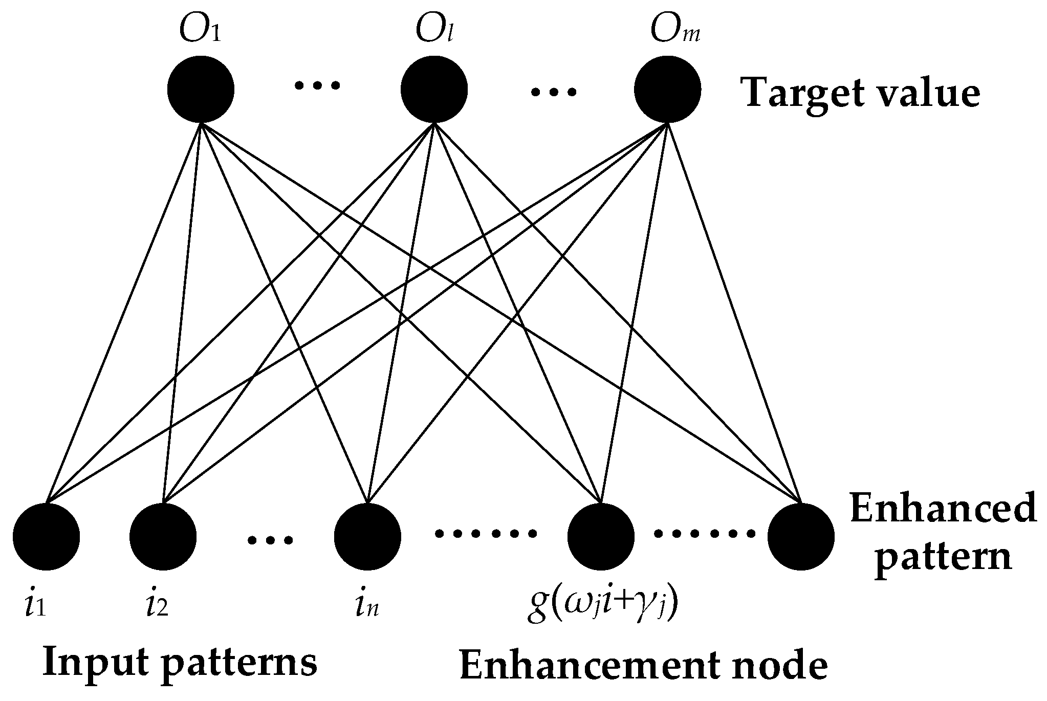
Ref. [34] proposed the random vector functional-link net (FLNet), where the input and output layers are directly connected without an activation function. At the same time, an enhanced pattern is employed as an alternative to the nonlinear activation function. The structure of FLNet used for phase space nonlinear mapping in this paper is illustrated in Figure 7.

$G(\cdot )$ is the randomly input activation function, representing the nonlinear part of the model, such as the sigmoid function and so on. ${\omega }_m\in R^{1\times (d+1)}$ is a parameter generated randomly from the 0–1 continuous uniform distribution to generate nonlinear effects in combination with the activation function, which is called the enhancement node, and m is the number of enhancement nodes. Compared with conventional neural network structures with nonlinear relationships, the structure adopted herein not only provides nonlinear characteristics that are not originally available for the mapping between phase space reconstruction vectors but is also more in line with engineering reality. At the same time, under the framework of this structure, the regression parameters can be directly calculated by linear regression formulas, which can eliminate calculations in neural networks that need to use gradient descent methods, thus exhibiting the superior advantage of small calculation amounts. In summary, when applying the phase space reconstruction function, the mapping between $y_R(n+1)$ and $y_R(n)$ can be rewritten as

$$\begin{array}{l}{y}_R(n+1)={\overline{A}}_{n}b\left(n\right)\\ b\left(n\right)={\left\{y_R^{\mathrm{T}}\left(n\right),G{\left[\theta \stackrel{⌢}{y}\left(n\right)\right]}^{\mathrm{T}},1\right\}}^{\mathrm{T}}\end{array}$$

(20)

where $\theta \in R^{m\times (d+1)}$ is a random parameter matrix generated from the continuous uniform distribution, which is composed of $\omega$; $b(n)\in R^{d+m+1}$ is the combination of the reconstruction vector and the enhancement node. In summary, by rewriting Equation (16) using Equation (20), the following can be obtained:

$$\begin{array}{l}{\overline{A}}_n=Y_{n+1}{\left(B_n\right)}^{\mathrm{T}}{\left[B_n{\left(B_n\right)}^{\mathrm{T}}\right]}^{-1}\\ B_n=\left[b^1\left(n\right)b^2\left(n\right)\dots b^I\left(n\right)\right]\end{array}$$

(21)

By combining Equations (19)–(21),

$$e_p\left(n\right)=y_p\left(n+1\right)-Y_{n+1}{\left(B_n\right)}^{\mathrm{T}}{\left[B_n{\left(B_n\right)}^{\mathrm{T}}\right]}^{-1}{\left\{y_R^{\mathrm{T}}\left(n\right),G{\left[\theta \stackrel{⌢}{y}\left(n\right)\right]}^{\mathrm{T}},1\right\}}^{\mathrm{T}}$$

(22)

Then, according to the Ref. [31], the final quantified damage state of the bearing in the phase space can be calculated using Equation (23).

$$\begin{array}{l}{q}_n=\frac{1}{r_n^M}\\ E_p=\sqrt{\frac{{\displaystyle {\sum }_{n=1}^{N}q\left(n\right){\Vert e_p\left(n\right)\Vert }^2}}{{\displaystyle {\sum }_{n=1}^{N}q\left(n\right)}}}\end{array}$$

(23)

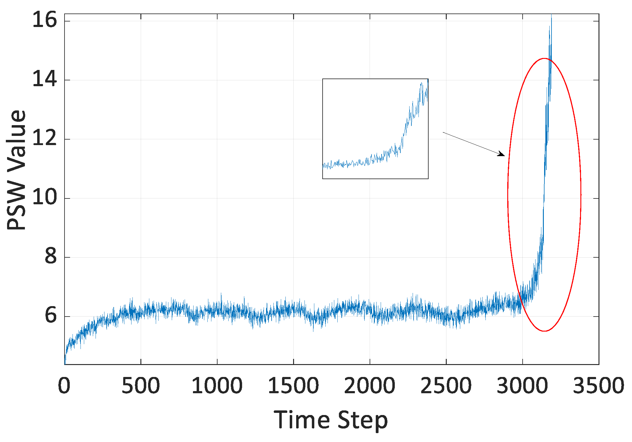
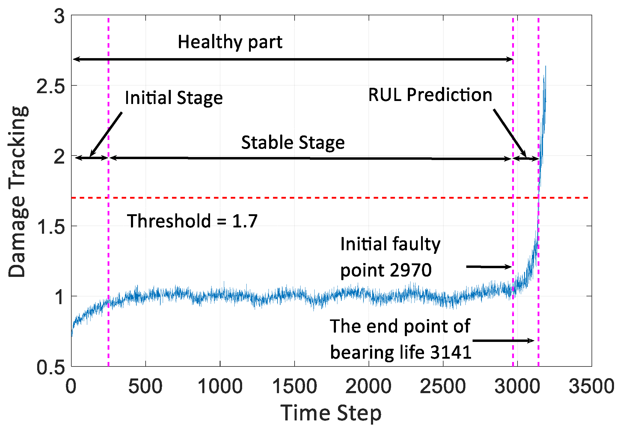
where $q(n)$ is the weight function. $r_n$ is the Euclidean distance between the current reconstruction vector $y_p(n)$ and the one that has the farthest Euclidean distance in the space composed of the I nearest neighbor vectors. M is the correlation dimension of the reference phase space. Finally, with the sample Bearing 1-1 as an example, the improved PSW results are shown in Figure 8. Compared with kurtosis and RMS, it exhibits significantly smaller fluctuations and better monotonicity, so it is more appropriate to serve as the health indicator for the bearing.

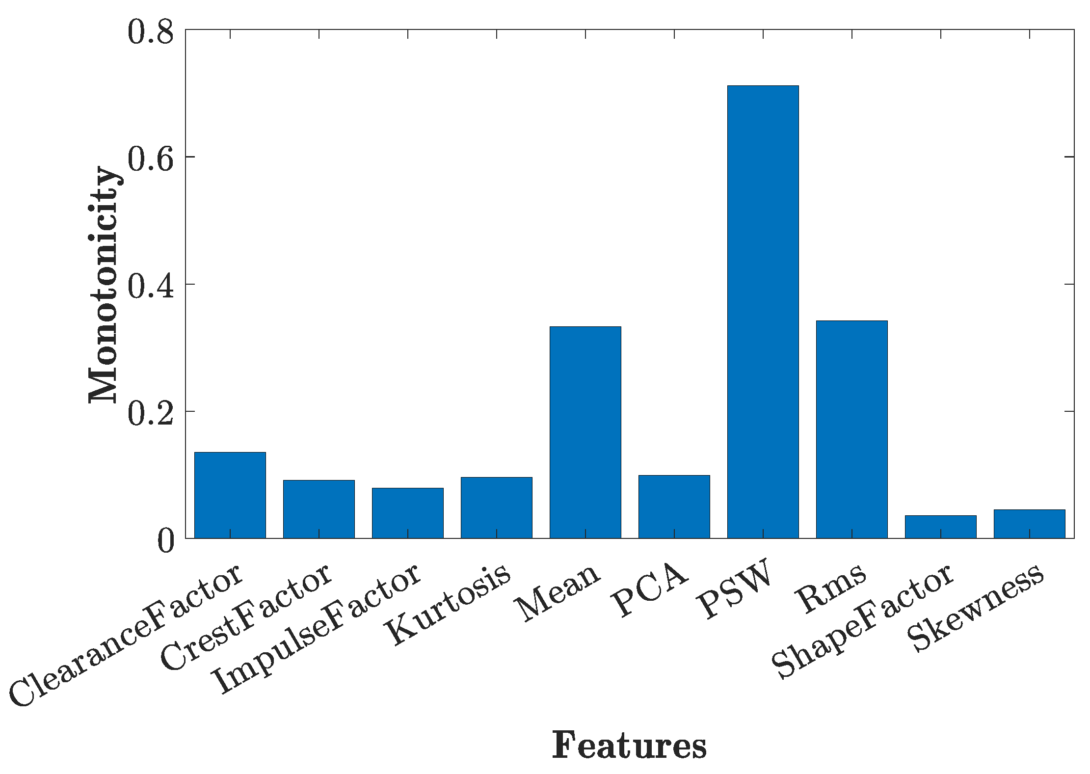
In Refs. [35,36], several other features shown in

Table 3. Statistical features.

Features	Definitions
Absolute mean	$F_{\mathrm{mean}}=\frac{1}{n}{\displaystyle {\sum }_{i=1}^n\left|x_i\right|}$
Root mean square	$F_{\mathrm{RMS}}=\sqrt{\frac{1}{n}{\displaystyle \sum _{i=1}^n{\left|x_i\right|}^2}}$
Kurtosis	$F_{\mathrm{KURT}}=\frac{1}{n}{\displaystyle \sum _{i=1}^n\frac{{\left(x_i-{\mu }_x\right)}^4}{{\sigma }_x^4}}$
Skewness	$F_{\mathrm{SKEW}}=\frac{1}{n}{\displaystyle \sum _{i=1}^n\frac{{\left(x_i-{\mu }_x\right)}^3}{{\sigma }_x^3}}$
Crest factor	$F_{\mathrm{CF}}=\frac{\left|\max \left(X\right)-\min \left(X\right)\right|}{2F_{\mathrm{RMS}}}$
Clearance factor	$F_{\mathrm{CLF}}=\frac{\left|\max (X)-\min (X)\right|}{2{\left(\frac{1}{n}{\displaystyle \sum _{i=1}^n{\left|x\right|}^{\frac{1}{2}}}\right)}^2}$
Impulse factor	$F_{\mathrm{IF}}=\frac{\left|\max (X)-\min (X)\right|}{2F_{\mathrm{mean}}}$
Shape factor	$F_{\mathrm{SF}}=\frac{F_{\mathrm{RMS}}}{F_{\mathrm{mean}}}$
PCA	Above features fused by PCA

are used for the prediction of bearing RUL. However, the prediction task begins after the occurrence of bearing initial damage. Hence, we select the monotonicity of the features after the bearing initial damage as the evaluation criterion. For a comparison purpose, the result from the PSW method is presented together with those from other features, as shown in Figure 9.

$$\mathrm{Monotonicity}=\frac{1}{n-1}{\displaystyle \sum _{i=1}^{n-1}\left[\mathrm{sgn}\left(x_{i+1}-x_i\right)\right]}$$

(24)

4. Feature Normalization

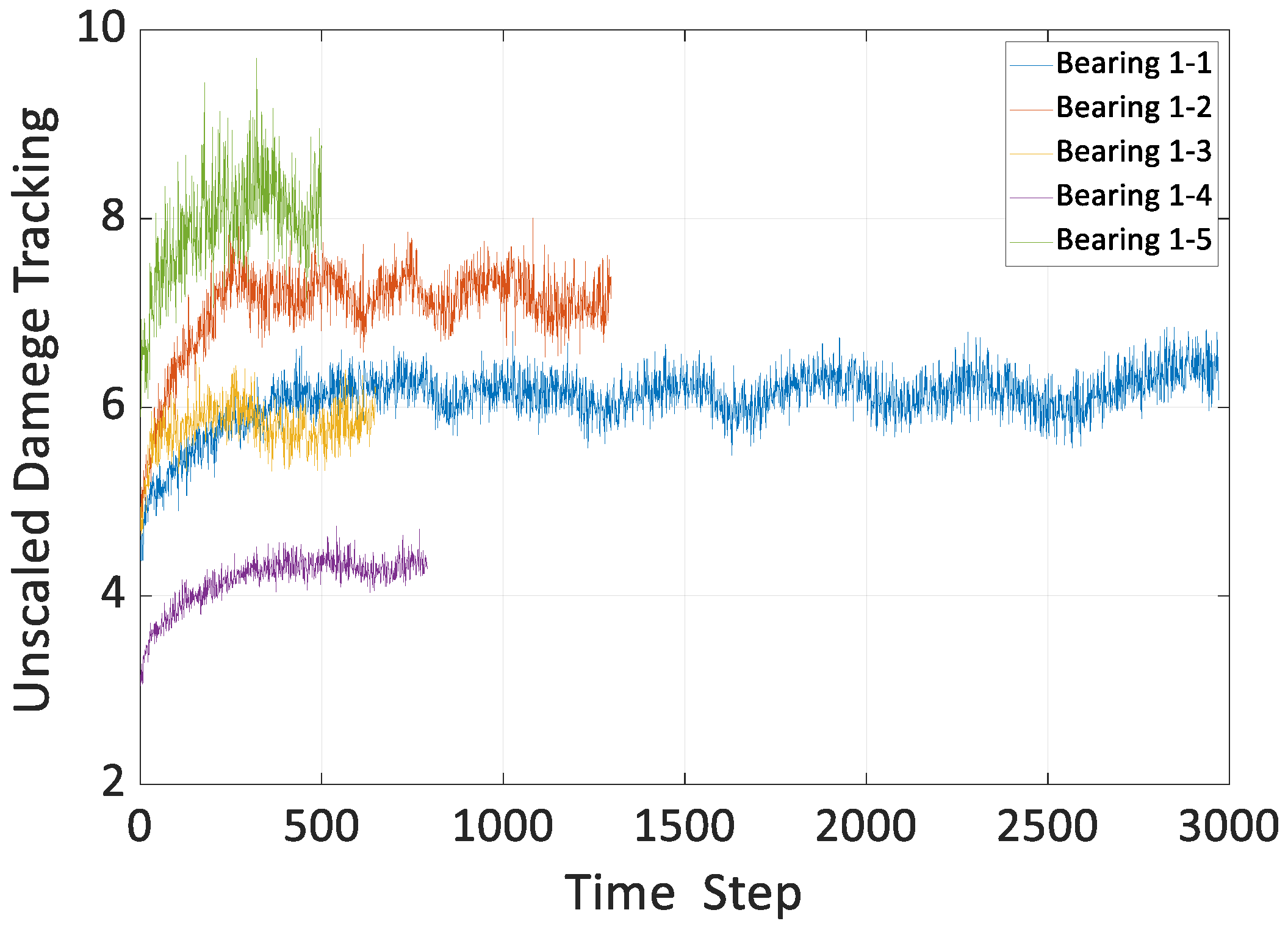
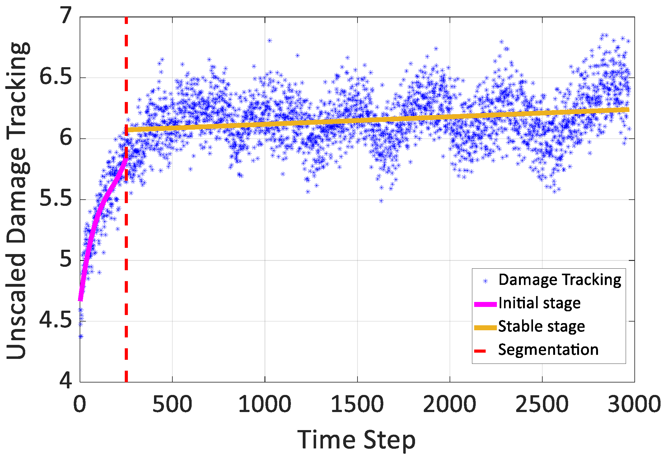
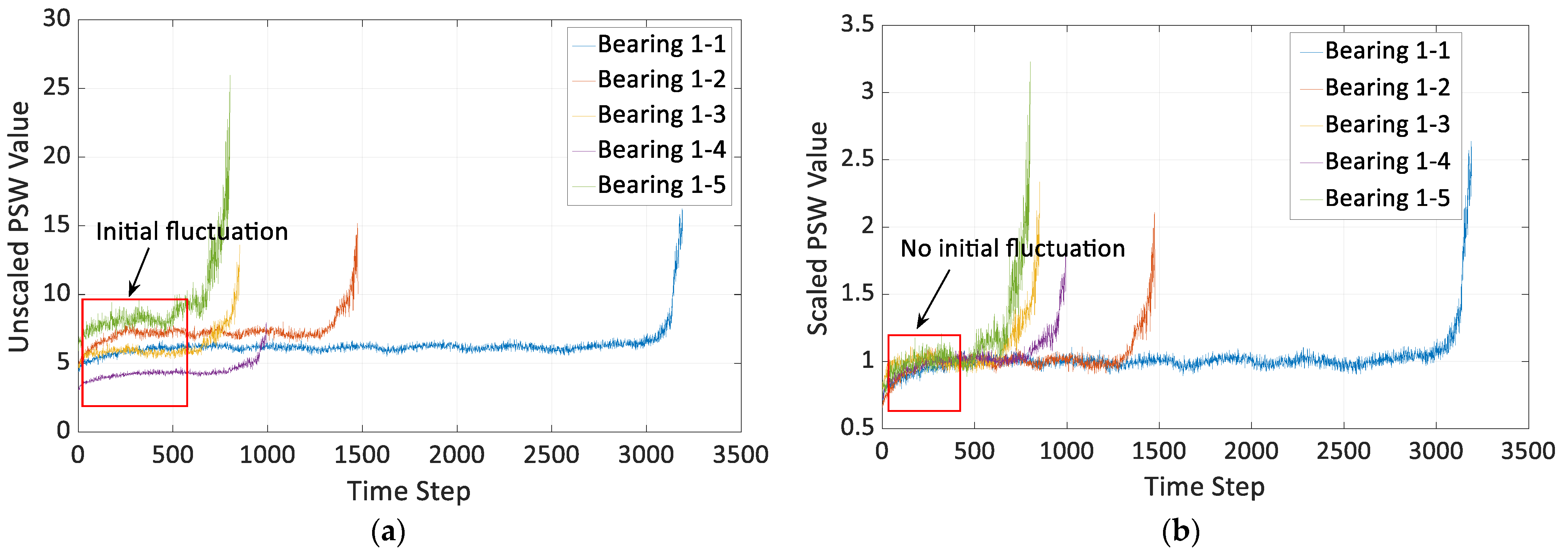
The improved PSW can better describe the damage state of the bearing from the perspective of the bearing system, but there are still certain problems with PSW for different bearings. Figure 10a shows the full life PSW data of five identical bearings under the same working conditions. There are relatively large initial fluctuations in the PSW values of different bearings. Similarly, the traditional RMS also faces the same problem. Therefore, it is necessary to develop a numerical standardization method to unify the quantitative standard of the bearing health indicator.

This study utilized a method proposed in the Ref. [9], which used relative values to unify and quantify health indicators. In this method, the relative PSW value is calculated as follows:

$$E_{\mathrm{scaled}}\left(t\right)=\frac{E\left(t\right)}{\frac{1}{h_1+h_2-1}{\displaystyle {\sum }_{h_1}^{h_2}E\left(h\right)}}$$

(25)

where h₁ and h₂ are the starting and ending point of the steady phase during the full life of the bearing. In Ref. [9], these two points were selected empirically, which is not a scientifically effective approach. In this paper, the ending point h₂ of the steady phase of the bearing is defined as the point of occurrence of minor faults; that is, the starting point of the fault obtained by the adaptive envelope analysis method described in Section 2. As for the starting point of the steady phase, Figure 10 indicates that once the bearing starts to operate, there is a certain “shift” in the bearing system state at the initial phase. However, this de facto “shift” is not damage; therefore, it is unreasonable to use the bearing’s starting point as the starting point of its steady phase. Therefore, this paper proposes to employ HMMR and use the PSW data before the fault point as its good input to perform unsupervised classification, thereby automatically dividing this segment of data into the initial phase and the steady phase.

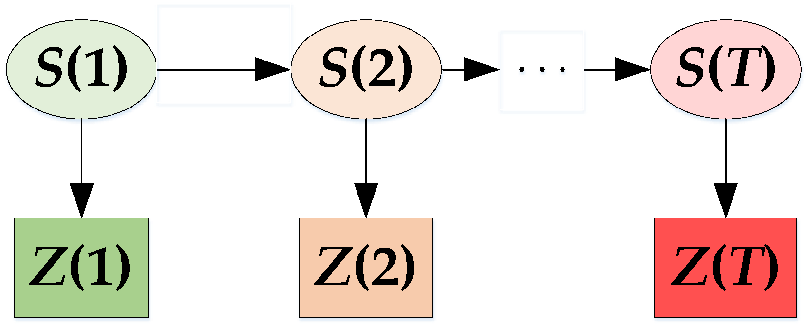
4.1. Hidden Markov Theory

The HMM model is a model for nested stochastic processes, which contains two states: one is the invisible hidden state $S(t)\in \left\{S_1,S_2\dots S_Q\right\}$, and the other is the explicit state $Z(t)\in \left\{Z_1,Z_2\dots Z_K\right\}$ based on the hidden state, as shown in Figure 11. Q and K are the number of hidden and explicit states, respectively.

The evolution of this model is generally described by the transition probability matrix A, which can be expressed as $A=\{a_{jj}\}=P[S(t+1)=S_j|S(t)=S_i]$, where i and j, respectively, represent the ith and jth hidden state, and $a_{ij}$ represents the transition probability from hidden state i to j. Under the current hidden state $S(t)$, the probability of showing the explicit state $Z(t)$ is expressed by the emission matrix $B=[b_j(k)]=P[Z(t)=Z_k|S(t)=S_j]$. The initial probability of the stochastic process is expressed by $\pi =\left[{\pi }_1,{\pi }_2\dots {\pi }_Q\right]$. In summary, the parameters contained in a complete HMM model are given as

$$\lambda =\left\{\pi ,A,B\right\}$$

(26)

4.2. HMMR-Based Normalization

In this study, after extracting the healthy data of the bearing, it is assumed that the healthy phase of the bearing can be divided into two phases—namely the initial running-in stage and the steady stage—and regarded as the hidden states of the HMM model [37]; moreover, this is an irreversible process. Thus, the transition matrix A can be expressed as

$$A=\left[\begin{array}{cc}{a}_{11}& 1-a_{11}\\ 0& 1\end{array}\right]$$

(27)

Figure 12 indicates that in the initial running-in stage, the bearing’s PSW value is in the form of an increasing cubic spline, while in the steady phase, it tends to be a stable straight line. Therefore, the explicit state is treated as a continuous Gaussian random distribution based on a polynomial regression model in this paper, rather than a traditional discrete emission matrix. This way, the traditional HMM model is modified into an HMMR model, where the running-in phase is a cubic spline Gaussian regression model, and the steady phase is a linear Gaussian regression model, as shown by Equation (28).

$$\begin{array}{l}{E}_t=U_j^{\mathrm{T}}{\nu }_j+{\sigma }_j\xi \\ b_j\left(Z\right)=P\left[Z|S\left(t\right)=S_j\right]=\frac{N\left(e_t;U_j^{\mathrm{T}}{v}_j,{\sigma }_j^2\right)}{{\displaystyle \sum _{q=1}^{Q}N\left(e_t;U_q^{\mathrm{T}}{v}_q,{\sigma }_q^2\right)}}\end{array}$$

(28)

where U_j is the regression coefficient of the $(l+1)$-dimensional lth order function under the jth hidden state. ${\nu }_j={[1,t_j,t_j^2\cdot \cdot \cdot t_j^p]}^{\mathrm{T}}$ is the regression input (i.e., time input) under the jth hidden state. $\xi \sim N(0,1)$ is the Gaussian distribution with zero mean and one standard deviation, ${\sigma }_j$ is the standard deviation of the regression model under the jth hidden state. Therefore, the parameters for the HMMR model in this paper are rewritten as follows:

$$\overline{\lambda }=\left(\pi ,A,U_1,U_2,{\sigma }_1,{\sigma }_2\right)$$

(29)

Finally, according to the maximum likelihood estimation algorithm, the model parameters can be obtained as

$$\begin{array}{l}L\left(\overline{\lambda };e_t\right)=\log p\left(e_t;\overline{\lambda }\right)\\ =\log \left\{{\displaystyle \sum _{S}p\left[S\left(1\right);\pi \right]}\cdot {\displaystyle \prod _{t=2}^{T}p\left[S\left(t\right)|S\left(t-1\right);A\right]\cdot }{\displaystyle \prod _{t=1}^{T}N\left[e_t;U_{S\left(t\right)}^T,{\sigma }_{S\left(t\right)}^2\right]}\right\}\end{array}$$

(30)

According to the method proposed in the Ref. [38], Equation (30) can be solved by the expectation–maximization (EM) algorithm. Its results are shown in Figure 13, where the service state of the healthy bearing is automatically divided into the initial running-in phase and the steady operating phase. The end of the initial running-in phase—that is, the starting point of the steady operation phase—will be finally regarded as the theoretical point h₁ in Equation (25). 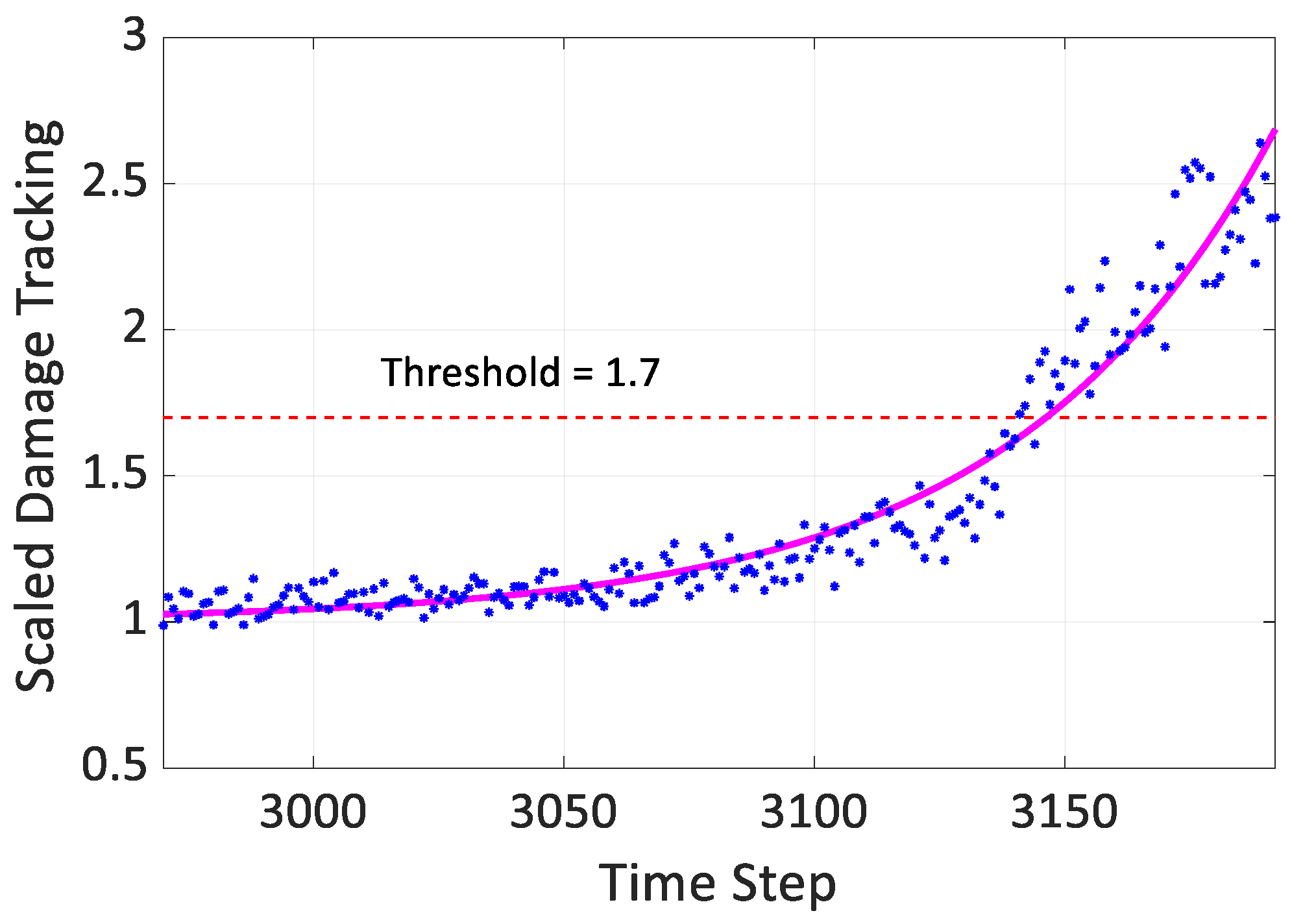Figure 10b shows the standardized result of the PSW data in Figure 10a obtained by the above method.

Figure 1 illustrates the crack length in the spall area to represent the damage degree of a specific damaged bearing. Multiple spall areas are also shown in Figure 1 and are represented as the identifier ‘+’ in Table 2. Damage related standardized PSW value is given in the same column of Table 2, together with RMS and kurtosis. Compared with the traditional RMS and kurtosis, an obvious positive correlation can be observed between the standardized PSW value and the crack length.

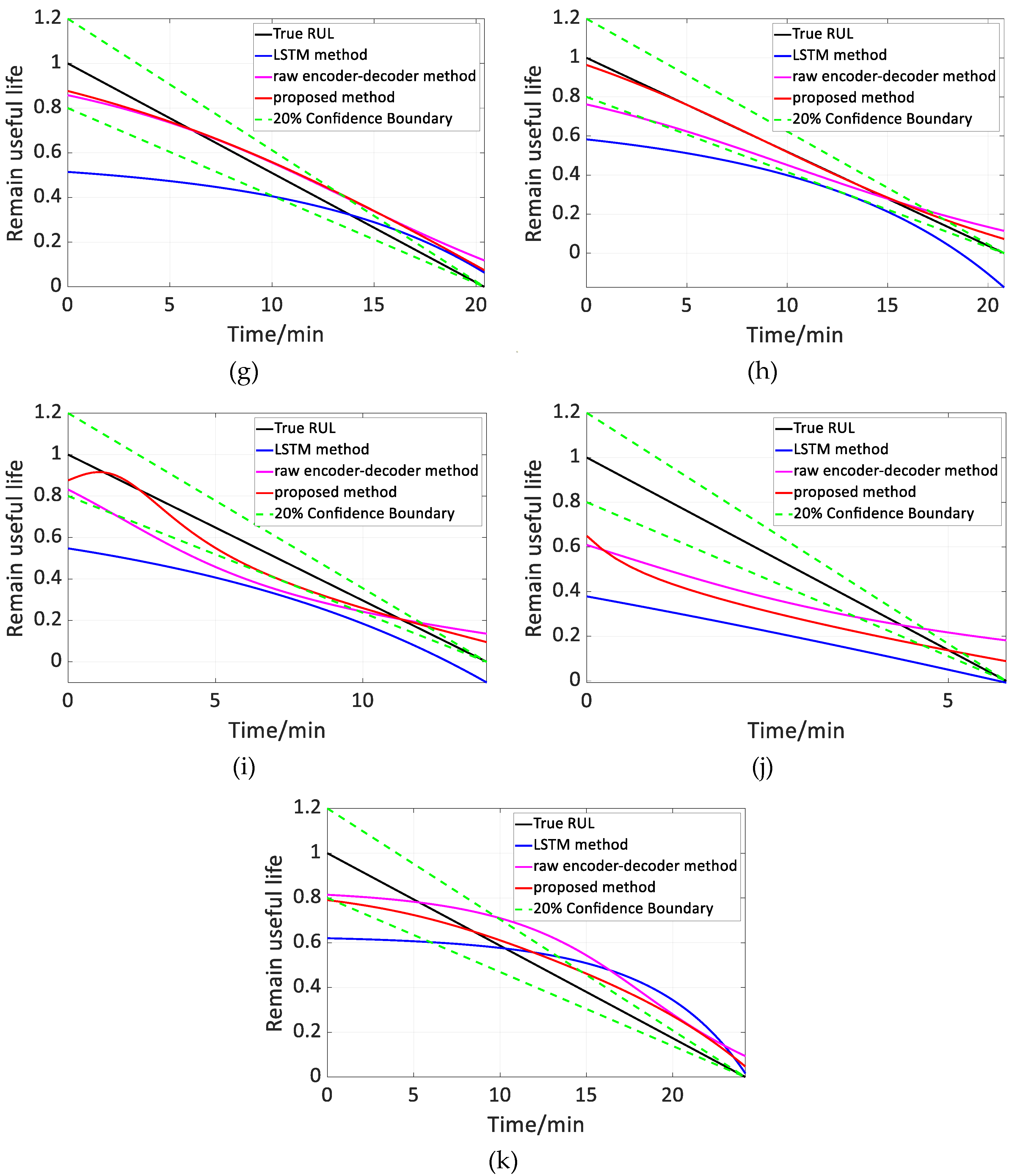
5. Bearing RUL Estimation

5.1. Ending Point of the Bearing Life

According to the theory introduced in the above sections, the standardized PSW indicator of the bearing can be obtained, and the starting point of the bearing’s minor fault can be accurately identified. Based on the above information, the bearing RUL can be predicted with the starting point of the bearing’s minor fault as the starting point. Table 2 indicates that there is a positive correlation between the bearing’s PSW indicator and its physical damage crack. Therefore, a PSW threshold indicator can be defined based on the above information to serve as the ending condition of bearing life. In this paper, this threshold is defined as Threshold = 1.7, as shown in Figure 14.

5.2. Feature Smoothing

To further reduce the error caused by feature fluctuations and to lower the influence of noise, exponential curve fitting is performed on the data before training the mathematical model for bearing RUL prediction [7,9]. The theoretical model is expressed as

$$y_E={\alpha }_E\exp \left({\beta }_{E}t\right)+{\gamma }_E$$

(31)

where ${\alpha }_E$, ${\beta }_E$, and ${\gamma }_E$ are the exponential curve fitting parameters. The fitting result is shown in Figure 15. Finally, the fitted data are input into the mathematical model presented in Section 5.3 for calculation. As shown in Figure 16, the method with exponential curve fitting has a better performance in predicting the bearing RUL against the method without curve fitting.

5.3. Bearing RUL Prediction

The LSTM model is a classic time series prediction network model [39]. This model consists of the following three components: forget gate, input gate, and output gate. In this model, the current hidden state H_t and the cell memory state C_t update on H_t−1 and C_t−1 based on the input I_t−1 of the previous time point according to the relevant algorithm. Finally, the time information of the time series is input. Its forward propagation process is expressed as follows:

$$\begin{array}{l}{\Gamma }_f=\mathrm{sigmoid}\left[W^f\left(H_{t-1},I_{t-1}\right)+b^f\right]\\ {\Gamma }_i=\mathrm{sigmoid}\left[W^i\left(H_{t-1},I_{t-1}\right)+b^i\right]\\ {\Gamma }_o=\mathrm{sigmoid}\left[W^o\left(H_{t-1},I_{t-1}\right)+b^o\right]\\ C_t=C_{t-1}\cdot {\Gamma }_f+\left\{{\Gamma }_i\cdot \tanh \left[W^c\left(H_{t-1},I_{t-1}\right)+b^c\right]\right\}\\ H_t={\Gamma }_o\cdot \tanh \left(C_t\right)\\ Z_t=H_t\end{array}$$

(32)

To enhance the prediction effectiveness of the LSTM model for bearing life, an LSTM-based encoder–decoder model [7] was proposed. To further improve the performance of the network, this paper sought to improve the model itself, such that in addition to introducing the attention mechanism reference, the bi-directional long-short term memory (BILSTM) was adopted to further extract the time information between bearing PSW indicators, and a residual model was also introduced to prevent gradient divergence. The calculation of the attention mechanism is shown by Equations (33)–(35).

$$C={\displaystyle {\sum }_{t=1}^{ti}{p}_t{H}_t^e}$$

(33)

$$p_t=\frac{\exp \left(s_t\right)}{{\displaystyle {\sum }_{t=1}^{ti}\exp \left(s_t\right)}}$$

(34)

$$S_t=\mathrm{Attention\; Function}\left(H_t^r,H_y^1\right)$$

(35)

where ti is the length of the input time series, and $H_y^1$ are, respectively, the result of the residual block hidden unit and the result of the first layer LSTM hidden unit of the decoder at the time t, $H_t^e$ is the result of the decoder hidden unit at the time t.

In the traditional LSTM model, the initial hidden unit H₀ is usually a zero matrix. However, in this model, the damage type and working condition of the bearing are used as the one-hot matrix and the hidden unit input, as illustrated in Figure 17.

Finally, combined with the PSW health indicators mentioned in this paper, the input and output of the entire network are given by Equation (36), where R_tn is the normalized life at the time T_n after standardization. Figure 18 depicts the flow chart of the entire life prediction process.

$$\begin{array}{c}\left[E_1,E_2,E_3,\cdot \cdot \cdot ,E_{ti-1},E_{ti}\right]\to R_1\\ \left[E_2,E_3,E_4,\cdot \cdot \cdot ,E_{ti},E_{ti+1}\right]\to R_2\\ \cdot \\ \cdot \\ \cdot \\ \left[E_{n-1},E_n,E_{n+1},\cdot \cdot \cdot ,E_{T_n+ti-3},E_{T_n+ti-2}\right]\to R_{T_n-1}\\ \left[E_n,E_{n+1},E_{n+2},\cdot \cdot \cdot ,E_{T_n+ti-2},E_{T_n+ti-1}\right]\to R_{T_n}\end{array}$$

(36)

6. Experimental Results

6.1. Description of the Test Rig

The bearing accelerated life test rig shown in Figure 19 is used for the experiment. In this test rig, the rotation of the shaft, test bearing, and support bearing are driven by a motor. The load on the test bearing is provided by the hydraulic loading system, and the vibration during bearing operation is measured using acceleration sensors.

The radial vibration of the bearing seat during the experiment is picked up by two horizontal and vertical PCB 608A11 acceleration sensors. The NI-9234 vibration acceleration acquisition card is used to acquire acceleration signals at a sampling frequency of 51.2 kHz. The sampling duration of each acquisition is 1.28 sec, and data are acquired every 12 sec. Section A sampling termination rule is formulated during the experiment––when any one of the two radial vibration accelerations exceeds 20 g, the test would be stopped immediately. The LDK-UER 205 bearing is used as the test bearing, and the corresponding geometric parameters are listed in Table 1. The test was carried out under three different working conditions, namely the rotation speed of 33 Hz/load of 800 kg, the rotation speed of 33 Hz/load of 900 kg, and the rotation speed of 33 Hz/load of 1000 kg. The tests are detailed in

Table 4. Experimental results and the tracking metric values when experiment ended.

Conditions	Dataset	Samples	Test Time	Faulty Type	Ended Tracking Metric
	Bearing 1-1	3192	10 h 38 min	Inner-race	2.64
	Bearing 1-2	1477	4 h 55 min	Inner-race	2.107
33 Hz-800 kg	Bearing 1-3	853	2 h 51 min	Inner-race	2.337
	Bearing 1-4	994	3 h 19 min	Inner-race	1.878
	Bearing 1-5	802	2 h 40 min	Inner-race	3.231
	Bearing 2-1	584	1 h 57 min	Roller	1.446
	Bearing 2-2	608	2 h 2 min	Inner-race	1.496
33 Hz-900 kg	Bearing 2-3	399	1 h 20 min	Outer-race	1.584
	Bearing 2-4	935	3 h 7 min	Inner-race	1.71
	Bearing 2-5	581	1 h 56 min	Inner-race	2.397
	Bearing 3-1	550	1 h 50 min	Inner-race	2.575
	Bearing 3-2	1238	4 h 8 min	Outer-race	3.61
33 Hz-1000 kg	Bearing 3-3	390	1 h 18 min	Inner-race	1.293
	Bearing 3-4	768	2 h 37 min	Inner-race	2.427
	Bearing 3-5	386	1 h 17 min	Inner-race	1.96

.

6.2. Experimental Results

In this experiment, it is defined that the life of the bearing is terminated only after the standardized PSW indicator exceeds 1.7. Therefore, based on the information in Table 4, only the 11 datasets including Bearing 1-1, Bearing 1-2, Bearing 1-3, Bearing 1-4, Bearing1-5, Bearing 2-4, Bearing 2-5, Bearing 3-1, Bearing 3-2, Bearing 3-4, and Bearing 3-5 are used as the final test sets. Further, the time series input length of the neural network is defined as ti = 20 herein. The final result is based on the prediction results obtained with each of the eleven data sets as the test set, as shown in Figure 20.

To quantitatively assess the accuracy of the model proposed in this paper, the RMS error (see Equation (37)) is used as the criterion.

$$\mathrm{RMSE}=\sqrt{\frac{1}{T_n-1}{\displaystyle {\sum }_{t=1}^{T_n}{\left(R_t-{\stackrel{⌢}{R}}_t\right)}^2}}$$

(37)

Table 5. RUL prediction errors of different methods.

Method	Average RMS Error
SVR	0.1164
3-Layer FC network	0.1440
LSTM	0.2127
TCN-LSTM	0.1895
Raw encoder-decoder	0.1052
Proposed method	0.0792

shows the average error of the eleven bearing datasets (see Figure 20), respectively, as the test sets, using several other methods, including SVR [9], 3-layer FC network, LSTM [40], TCN-LSTM [41] and raw encoder-decoder model [7].

7. Conclusions

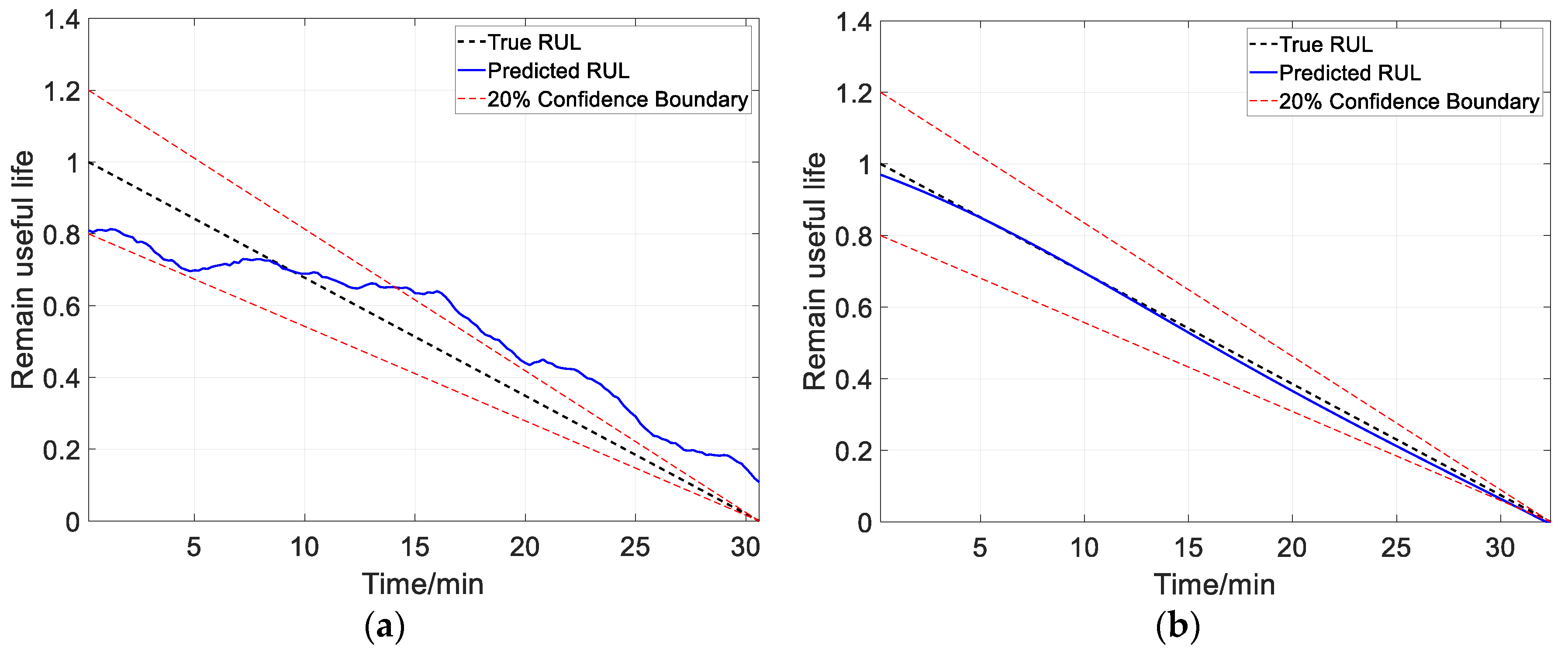
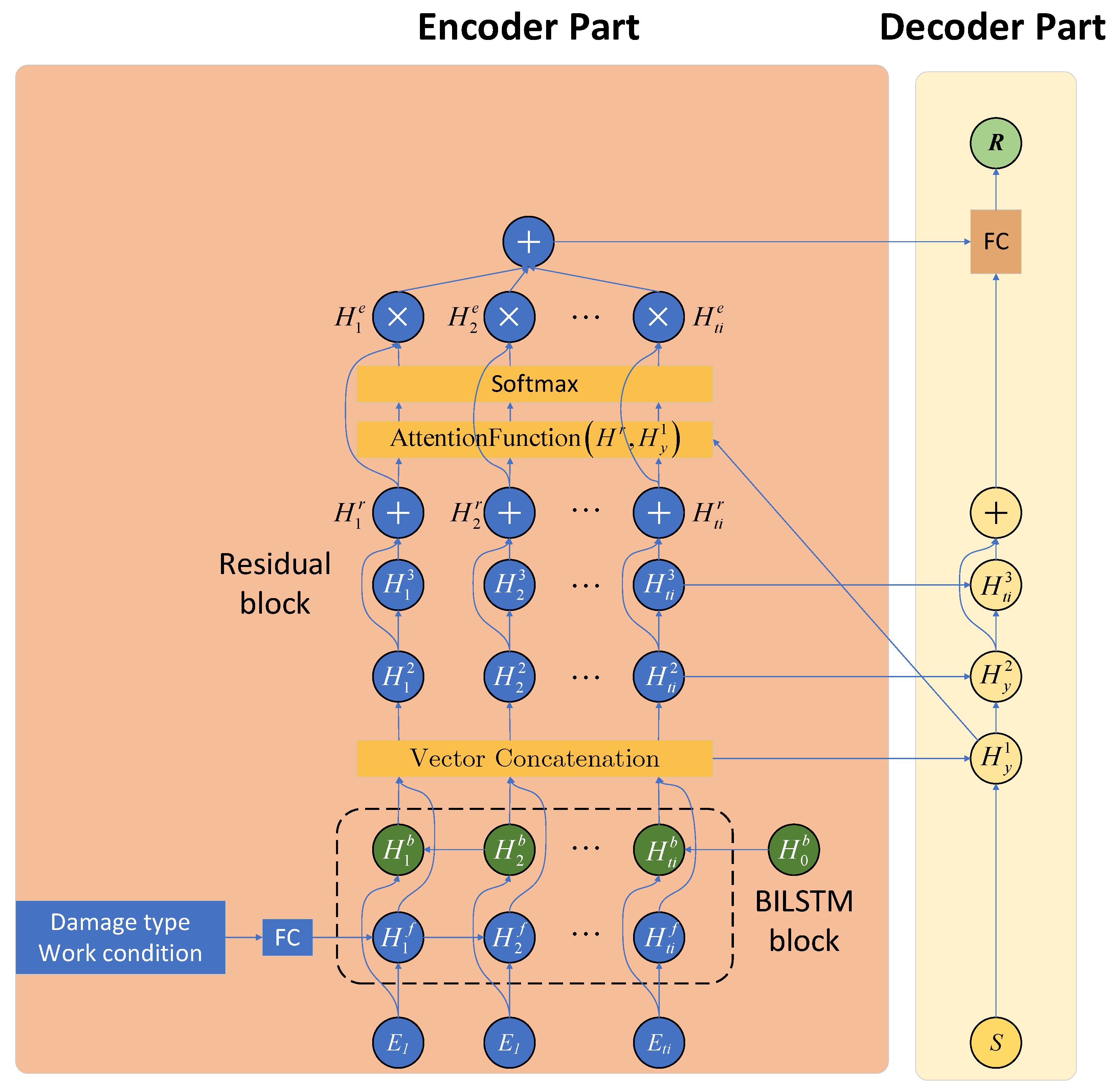
Most extant studies on the RUL prediction of rolling bearings have limited themselves to online public data sets, which do not consider the actual damage degree of the bearing and also rarely consider the starting and ending points for the bearing RUL prediction or the damage type of the bearing. Compared with the traditional health indicators used for life prediction, the standardized PSW indicator based on HMMR and improved PSW proposed in this paper can effectively evaluate the actual damage size in the bearing. Moreover, it was experimentally verified that with this indicator as input, the encoder–decoder neural network that combines the attention mechanism (which takes into account the bearing damage type and working conditions) and the BILSTM model can effectively improve the prediction accuracy for bearing RUL, thereby generating certain engineering value.

The main contributions of this paper are summarized as follows:

Instead of using the traditional statistical life distribution to predict the bearing life, the damage starting time point for bearing life prediction is accurately defined from the perspective of the characteristic frequency of the rolling bearing through the adaptive envelope analysis method.

A health indicator that can effectively reflect the actual damage of the bearing is obtained by combining the HMMR model and the PSW model.

Compared with the traditional LSTM model, the encoder–decoder LSTM model proposed in this paper considers the timing signal characteristic of the health indicator. Not only are the BILSTM model and attention mechanism introduced into the model, but also the operating conditions of the bearing are considered as the LSTM hidden state input for the calculation, thereby improving the prediction accuracy for bearing RUL.

References

1. Lei, Y.; Li, N.; Guo, L.; Li, N.; Yan, T.; Lin, J. Machinery health prognostics: A systematic review from data acquisition to RUL pre-diction. Mech. Syst. Signal. Process. 2018, 104, 799–834. [Google Scholar] [CrossRef]
2. Dias, M.H.; Azevedo, D.; Araújo, A.M.; Bouchonneau, N. A review of wind turbine bearing condition monitoring: State of the art and challenges. Renew. Sustain. Energy Rev. 2016, 56, 368–379. [Google Scholar]
3. IEEE PHM 2012 Prognostic Challenge. Outline, Experiments, Scoring of Results, Winners. Available online: http://www.femto-st.fr/f/d/IEEEPHM2012-Challenge-Details.pdf (accessed on 27 September 2021).
4. Wang, B.; Lei, Y.; Li, N.; Li, N. A hybrid prognostics approach for estimating remaining useful life of rolling element bear-ings. IEEE Trans. Reliab. 2020, 69, 401–412. [Google Scholar] [CrossRef]
5. Qiu, H.; Lee, J.; Lin, J.; Yu, G. Wavelet filter-based weak signature detection method and its application on rolling element bearing prognostics. J. Sound Vib. 2006, 289, 1066–1090. [Google Scholar] [CrossRef]
6. Kundu, P.; Darpe, A.K.; Kulkarni, M.S. Weibull accelerated failure time regression model for remaining useful life prediction of bearing working under multiple operating conditions. Mech. Syst. Signal. Process. 2019, 134, 106302. [Google Scholar] [CrossRef]
7. Liu, L.; Song, X.; Chen, K.; Hou, B.; Chai, X.; Ning, H. An enhanced encoder–decoder framework for bearing remaining useful life prediction. Measurement 2021, 170, 108753. [Google Scholar] [CrossRef]
8. Huang, G.; Zhang, Y.; Ou, J. Transfer remaining useful life estimation of bearing using depth-wise separable convolution re-current network. Measurement 2021, 176, 109090. [Google Scholar] [CrossRef]
9. Yan, M.; Wang, X.; Wang, B.; Chang, M.; Muhammad, I. Bearing remaining useful life prediction using support vector machine and hybrid degradation tracking model. ISA Trans. 2020, 98, 471–482. [Google Scholar] [CrossRef] [PubMed]
10. Wang, B.; Lei, Y.; Li, N.; Yan, T. Deep separable convolutional network for remaining useful life prediction of machinery. Mech. Syst. Signal. Process. 2019, 134, 106330. [Google Scholar] [CrossRef]
11. Li, N.; Lei, Y.; Lin, J.; Ding, S.X. An Improved Exponential Model for Predicting Remaining Useful Life of Rolling Element Bearings. IEEE Trans. Ind. Electron. 2015, 62, 7762–7773. [Google Scholar] [CrossRef]
12. Huang, Z.; Xu, Z.; Ke, X.; Wang, W.; Sun, Y. Remaining useful life prediction for an adaptive skew-Wiener process model. Mech. Syst. Signal. Process. 2017, 87, 294–306. [Google Scholar] [CrossRef]
13. Zhong, J.; Wang, D.; Li, C. A nonparametric health index and its statistical threshold for machine condition monitoring. Measurement 2021, 167, 108290. [Google Scholar] [CrossRef]
14. Xu, L.; Pennacchi, P.; Chatterton, S. A new method for the estimation of bearing health state and remaining useful life based on the moving average cross-correlation of power spectral density. Mech. Syst. Signal. Process. 2020, 139, 106617. [Google Scholar] [CrossRef] [Green Version]
15. Paris, P.C.; Erdogan, F. A critical analysis of crack propagation laws. J. Basic Eng. 1963, 85, 528–533. [Google Scholar] [CrossRef]
16. Kumar, P.S.; Kumaraswamidhas, L.A.; Laha, S.K. Bearing degradation assessment and remaining useful life estimation based on Kullback-Leibler divergence and Gaussian processes regression. Measurement 2021, 174, 108948. [Google Scholar] [CrossRef]
17. Qiu, G.Q.; Gu, Y.K.; Chen, J.J. Selective health indicator for bearings ensemble remaining useful life prediction with genetic algorithm and Weibull proportional hazards model. Measurement 2020, 150, 107097. [Google Scholar] [CrossRef]
18. Xing, J.; Zeng, Z.; Zio, E. A framework for dynamic risk assessment with condition monitoring data and inspection data. Reliab. Eng. Syst. Saf. 2019, 191, 106552. [Google Scholar] [CrossRef] [Green Version]
19. Li, J.; Zhang, X.; Zhou, X.; Lu, L. Reliability assessment of wind turbine bearing based on the degradation-Hidden-Markov model. Renew. Energy 2019, 132, 1076–1087. [Google Scholar] [CrossRef]
20. Pan, Z.; Meng, Z.; Chen, Z.; Gao, W.; Shi, Y. A two-stage method based on extreme learning machine for predicting the remain-ing useful life of rolling-element bearings. Mech. Syst. Signal. Process. 2020, 144, 106899. [Google Scholar] [CrossRef]
21. Chen, C.; Zhang, B.; Vachtsevanos, G.J.; Orchard, M. Machine Condition Prediction Based on Adaptive Neuro–Fuzzy and High-Order Particle Filtering. IEEE Trans. Ind. Electron. 2010, 58, 4353–4364. [Google Scholar] [CrossRef]
22. Singleton, R.K.; Strangas, E.G.; Aviyente, S. Extended Kalman Filtering for Remaining-Useful-Life Estimation of Bearings. IEEE Trans. Ind. Electron. 2015, 62, 1781–1790. [Google Scholar] [CrossRef]
23. Antoni, J. The infogram: Entropic evidence of the signature of repetitive transients. Mech. Syst. Signal. Process. 2016, 74, 73–94. [Google Scholar] [CrossRef]
24. Chegini, S.N.; Manjili, M.J.H.; Ahmadi, B.; Amirmostofian, I.; Bagheri, A. New bearing slight degradation detection approach based on the periodicity intensity factor and signal processing methods. Measurement 2021, 170, 108696. [Google Scholar] [CrossRef]
25. Nirwan, N.W.; Ramani, H.B. Condition monitoring and fault detection in roller bearing used in rolling mill by acoustic emis-sion and vibration analysis. Mater. Today Proc. 2021. [Google Scholar] [CrossRef]
26. Antoni, J. Fast computation of the kurtogram for the detection of transient faults. Mech. Syst. Signal. Process. 2007, 21, 108–124. [Google Scholar] [CrossRef]
27. Peeters, C.; Antoni, J.; Helsen, J. Blind filters based on envelope spectrum sparsity indicators for bearing and gear vibra-tion-based condition monitoring. Mech. Syst. Signal. Process. 2020, 138, 106556. [Google Scholar] [CrossRef]
28. Klausen, A.; Robbersmyr, K.G.; Karimi, H.R. Autonomous bearing fault diagnosis method based on envelope spectrum. IFAC-Pap. 2017, 50, 13378–13383. [Google Scholar] [CrossRef]
29. Zhang, H.; Borghesani, P.; Smith, W.A.; Randall, R.B.; Shahriar, R.; Peng, Z. Tracking the natural evolution of bearing spall size using cyclic natural frequency perturbations in vibration signals. Mech. Syst. Signal. Process. 2021, 151, 107376. [Google Scholar] [CrossRef]
30. Boštjan, D.; Pavle, B.; Đani, J. Distributed bearing fault diagnosis based on vibration analysis. Mech. Syst. Signal. Process. 2016, 66–67, 521–532. [Google Scholar]
31. Chelidze, D.; Cusumano, J.P.; Chatterjee, A. A Dynamical Systems Approach to Damage Evolution Tracking, Part 1: Description and Experimental Application. J. Vib. Acoust. 2002, 124, 250–257. [Google Scholar] [CrossRef] [Green Version]
32. Fraser, A.; Swinney, H.L. Independent coordinates for strange attractors from mutual information. Phys. Rev. A 1986, 33, 1134–1140. [Google Scholar] [CrossRef] [PubMed]
33. Cao, L. Practical method for determining the minimum embedding dimension of a scalar time series. Phys. D Nonlinear Phenom. 1997, 110, 43–50. [Google Scholar] [CrossRef]
34. Pao, Y.H.; Park, G.H.; Sobajic, D.J. Learning and generalization characteristics of the random vector Functional-link net. Neu-Rocomputing 1996, 6, 163–180. [Google Scholar] [CrossRef]
35. Zhang, Y.; Martínez-García, M.; Latimer, A. Selecting optimal features for cross-fleet analysis and fault diagnosis of industrial gas turbines. In Proceedings of the ASME Turbo Expo 2018: Turbomachinery Technical Conference and Exposition, Olso, Norway, 11–15 June 2018. [Google Scholar]
36. He, J.; Yang, S.; Papatheou, E.; Xiong, X.; Wan, H.; Gu, X. Investigation of a multi-sensor data fusion technique for the fault diagnosis of gearboxes. Proc. Inst. Mech. Eng. Part. C J. Mech. Eng. Sci. 2019, 233, 4764–4775. [Google Scholar] [CrossRef]
37. Rabiner, L.R. A tutorial on hidden Markov models and selected applications in speech recognition. Proc. IEEE 1989, 77, 257–286. [Google Scholar] [CrossRef]
38. Chamroukhi, F.; Samé, A.; Govaert, G.; Aknin, P. Time series modeling by a regression approach based on a latent process. Neural Netw. 2009, 22, 593–602. [Google Scholar] [CrossRef] [PubMed] [Green Version]
39. Hochreiter, S.; Schmidhuber, J. Long short-term memory. Neural Comput. 1997, 9, 1735–1780. [Google Scholar] [CrossRef]
40. Martínez-García, M.; Zhang, Y.; Suzuki, K.; Zhang, Y.D. Deep recurrent entropy adaptive model for system reliability moni-toring. IEEE Trans. Ind. Inform. 2021, 17, 839–848. [Google Scholar] [CrossRef]
41. Bai, S.J.; Kolter, J.Z.; Koltun, V. An empirical evaluation of generic convolutional and recurrent networks for sequence model-ing. arXiv 2018, arXiv:1803.01271. [Google Scholar]
Figure 1. Illustrations of crack length in the spall area to represent the damage degree of a bearing.
Machines 09 00238 g001
Figure 2. Adaptive band selection of envelope analysis based on local minimums of PSDs.
Machines 09 00238 g002
Figure 3. Eleven envelope spectrums of the inner-ring damage bearing obtained from the adaptive band selection, i.e., (ak) the envelope spectrum with the lowest enveloped band to the envelope spectrum with the highest enveloped band.
Machines 09 00238 g003
Figure 4. Eleven envelope spectrums of the outer-ring damage bearing obtained from the adaptive band selection, i.e., (ak) the envelope spectrum with the lowest enveloped band to the envelope spectrum with the highest enveloped band.
Machines 09 00238 g004
Figure 5. The zoom-in envelope spectrums of inner- and outer-ring damaged bearing, in which the calculated results of (a) the BPFI and its sidebands from our method, (b) the BPFO from our method, (c) the BPFI and its sidebands from the fast Kurtogram and (d) the BPFO from the fast Kurtogram.
Machines 09 00238 g005aMachines 09 00238 g005b
Figure 6. Trends of the statistical characteristics, i.e., (a) RMS and (b) kurtosis, against time step of Bearing 1-1.
Machines 09 00238 g006
Figure 7. Random vector functional-link net.
Machines 09 00238 g007
Figure 8. Damage tracking of Bearing 1-1.
Machines 09 00238 g008
Figure 9. Monotonicity of different features.
Machines 09 00238 g009
Figure 10. Unscaled PSW and scaled PSW. (a) Damaged tracking without scaling and (b) Damaged tracking with scaling.
Machines 09 00238 g010
Figure 11. HMM model.
Machines 09 00238 g011
Figure 12. Unscaled damage tracking in healthy stage.
Machines 09 00238 g012
Figure 13. Healthy stage segmentation of Bearing 1-1.
Machines 09 00238 g013
Figure 14. Illustration of RUL prediction.
Machines 09 00238 g014
Figure 15. Fitting result of unhealthy stage.
Machines 09 00238 g015
Figure 16. Effectiveness of exponential curve fitting for bearing RUL prediction. (a) Results without exponential curve fitting and (b) Results with exponential curve fitting.
Machines 09 00238 g016
Figure 17. Illustration of proposed network.
Machines 09 00238 g017
Figure 18. Flowchart of RUL prediction.
Machines 09 00238 g018
Figure 19. Accelerated endurance test rig of bearing RUL.
Machines 09 00238 g019
Figure 20. Prediction results of bearing RUL from different bearing datasets, which are respectively (a) Bearing 1-1, (b) Bearing 1-2, (c) Bearing 1-3, (d) Bearing 1-4, (e) Bearing 1-5, (f) Bearing 2-4, (g) Bearing 2-5, (h) Bearing 3-1, (i) Bearing 3-2, (j) Bearing 3-4, and (k) Bearing 3-5.
Machines 09 00238 g020aMachines 09 00238 g020b