1. Introduction
Thanks to digitization and Industry 4.0 technologies and solutions, today’s economy is in the middle of significant transformation processes regarding the fulfilment of customers’ demands. Production companies must apply the solutions of the fourth industrial revolution to improve their efficiency. The ever-changing production and service sector requires the improvement of these attributes. Logistics and material handling operations have more and more importance related to the purchasing, production, distribution, and reverse processes, and they have a significant impact on the strategic, tactical, and operative level of enterprise systems.
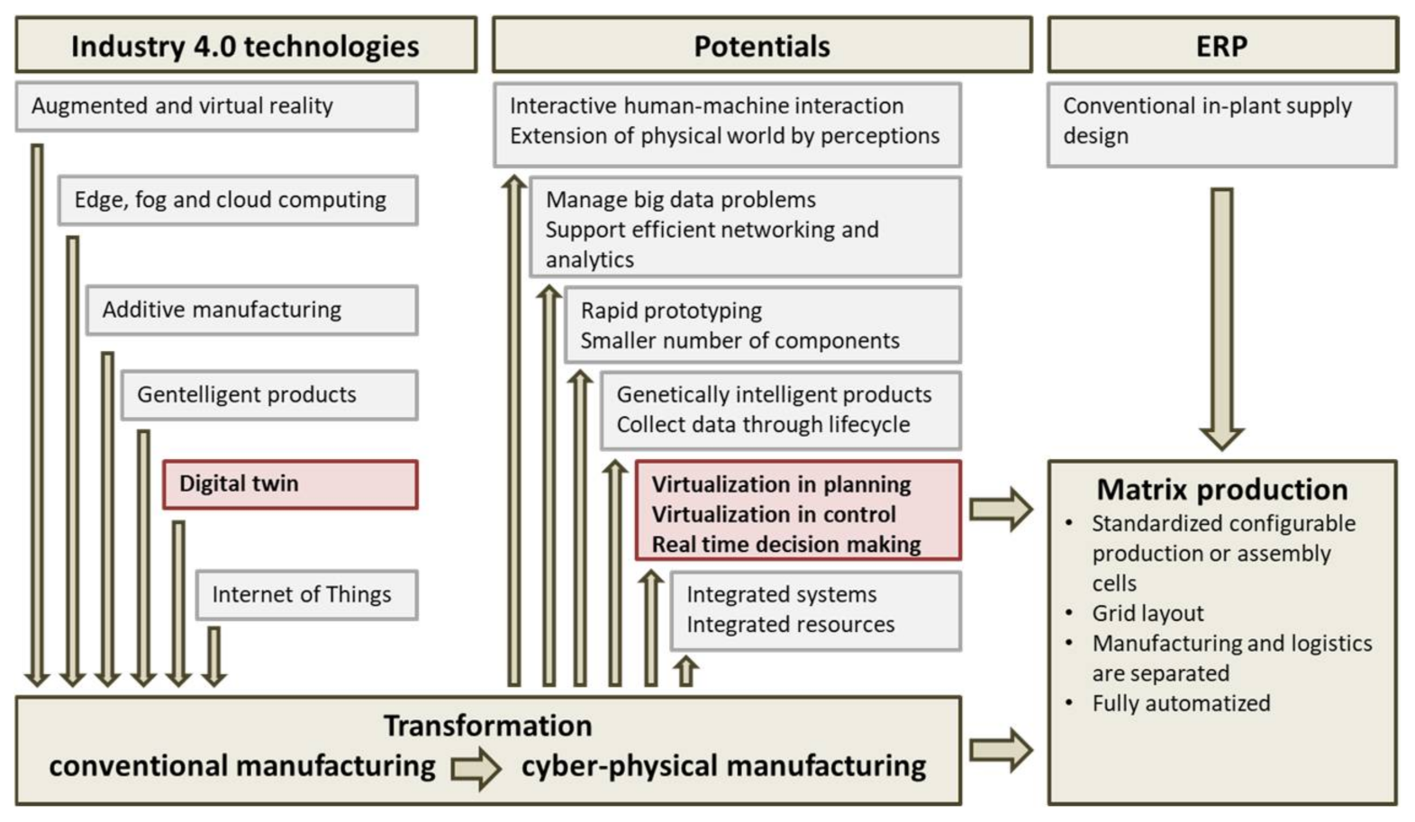
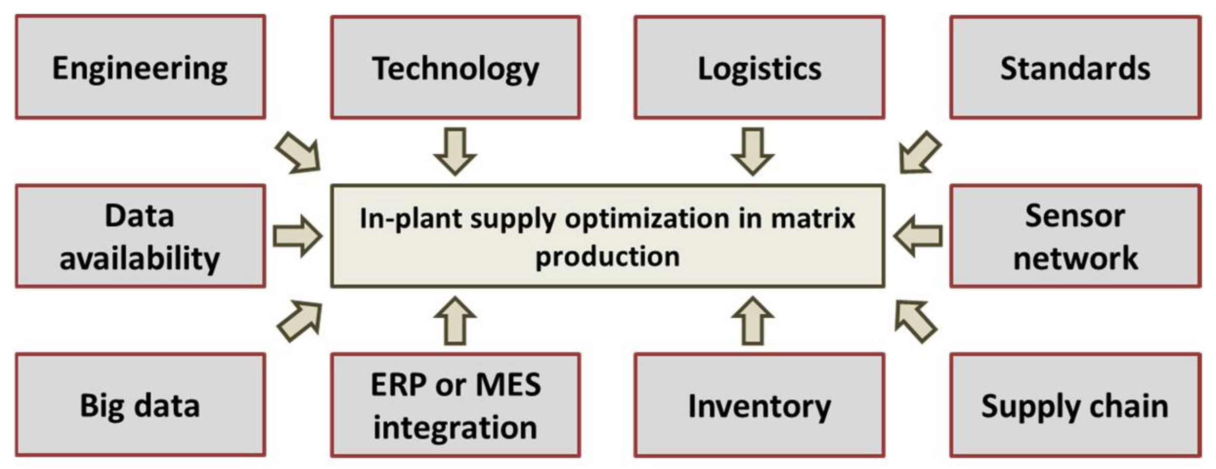
As
Figure 1 shows, Industry 4.0 technologies offer new innovation accelerators, like augmented and virtual reality, cloud and fog computing related to big data problems, additive manufacturing, Internet of Thing (IoT), autonomous standardized production and material handling resources, smart tools, gentelligent products, simulation and digital twin solutions, cyber security, and system integration. These Industry 4.0 technologies are important influencing factors for manufacturing processes [
1,
2] and they lead to the appearance of dynamic manufacturing networks [
3].
Augmented and virtual reality is a key technology for smart manufacturing because it makes it possible to realize an interactive human–machine interaction in a real-world environment while the components of the physical world are extended by perceptual information. Augmented and virtual reality can be used in training, design, manufacturing, operation, services, sales, and marketing. In the field of manufacturing, the most important applications are quality control and total quality management; maintenance operations, especially in a dangerous environment; assembly work instructions; and performance monitoring [
4].
Complex manufacturing systems generate unprecedented amounts of data that are difficult to handle with traditional computing methods. Cloud, edge, and fog computing make it possible to manage big data problems. Big data is coming from a wide range of sensors from manufacturing systems. Cloud and fog computing integrate servers, storages, databases to support efficient networking, analytics, and intelligence solutions [
5].
The introduction of additive manufacturing will have a great impact on the supply chain processes and logistics solutions, because both external and in-plant material flow solutions will change dramatically. It is caused by the fact that this technology is based on the building of 3D objects by adding layer-upon-layer of various materials, like plastic, metal, or organic materials [
6].
The new concept of gentelligent products aims to develop genetically intelligent products and components, which collect data through their lifecycle and bequeath them to the next generation in various time spans. The appearance of gentelligent products has a great impact on big data problems [
7].
The application of digitalization-based technologies enables the virtualization of product and process planning and control [
8]. Digital twins represent an integrated probabilistic simulation of complex products or processes using physical models, sensor updates, and cloud-based information to mirror the product or process of its corresponding twin [
9,
10]. Digital twin technology makes it possible to convert conventional manufacturing systems into cyber-physical systems, and this transformation can lead to the improvement of the design process of in-plant material supply, adding a real-time phase to the conventional in-plant supply process. In conventional manufacturing systems, the real time optimization is almost impossible, because real time optimization is based on real time data and status information. Using digital twin technology and smart sensor networks, real time data and status information can be collected from the physical system, and a real time model for discrete event simulation can be generated to perform scenario analysis for real time decision making.
The Internet of Things describes an integrated system of computers and mechanical machines provided with unique identifiers. The IoT in manufacturing systems makes it possible to transfer data through a network among manufacturing equipment (standardized production cells and assembly cells), materials handling machines (autonomous mobile robots and automated guided vehicles), intelligent tools, gentelligent products, and ERP systems [
11].
The Industry 4.0 technologies make it possible to transform conventional manufacturing processes to cyber-physical manufacturing processes to aim for higher flexibility, productivity, availability, cost-efficiency, energy-efficiency, and sustainability. The fulfilment of more and more diverse customers’ demands requires more and more sophisticated, flexible, and intelligent solutions based on these technologies both inside and outside of the production plants in all fields of industry including automotive industry as a flagship.
The in-plant material supply solutions are commonly based on milk-run material supply, especially in the field of automotive industry. KUKA AG (one of the world’s leading specialists in automation) offered a new, revolutionary solution for flexible manufacturing, transforming conventional manufacturing into cyber-physical manufacturing with the application of Industry 4.0 technologies. This new solution is the matrix production. With its new demonstration plant opened on March 2018 in Augsburg, KUKA demonstrates the advantages of this matrix production under real conditions. In a matrix production system, standardized configurable production or assembly cells are arranged in a grid layout. Manufacturing and logistics are separated and fully automatized. The matrix production system uses various Industry 4.0 technologies, like robots and turntables in the production and assembly cells, autonomous guided vehicles, digital twin support for real time control, prediction, and performance analysis. However, as a journalist wrote [
12], “However, all theory is gray.” There is a huge number of open questions focusing on manufacturing and logistics.
Manufacturing systems of increased complexity face a number of new design and operation problems that can be addressed by the opportunities provided by the Fourth Industrial Revolution. In the case of matrix production, the material supply of standardized configurable production or assembly cells is one of the most important tasks of logistics, because the separated manufacturing and logistics and the increased flexibility require new models and methods. This article focuses on the optimization of in-plant supply in matrix production. The highlights of the article are the following: (1) integrated model to solve the in-plant material supply problem in matrix production system, which enables both the conventional and real time planning of in-plant material supply; (2) integrated solution of assignment and routing problems based on heuristic optimization algorithms.
The article is organized as follows.
Section 2 presents a systematic literature review, which summarizes the research background of in-plant supply optimization in manufacturing systems.
Section 3 is the problem description including the mathematical model of integrated assignment and routing problem in matrix production systems.
Section 4 presents a metaheuristic optimization algorithm to solve the integrated assignment and routing problem, based on flower pollination and black hole heuristics.
Section 5 demonstrates the numerical results. Conclusions, managerial impacts, and future research directions are discussed in the remaining part of the article.
2. Literature Review
Within the frame of the systematic literature, the main scientific results, scientific gaps, and bottlenecks are identified and described [
13]. The optimization of logistics and supply chain design and control of manufacturing systems has been researched in the past 30 years. The first articles in this field were published before 2000, focusing on heuristic optimization of rough-mill yield with production priorities [
14], optimum allocation of jobs on machine-tools [
15], and facility location problem for large-scale logistics [
16]. The number of published research papers has increased; it shows the importance of the optimization of manufacturing-related supply chain solutions.
The literature introduces a wide range of design methods used to solve problems of manufacturing-related processes, like unified decomposition, decision-making methods, queuing theory, data-driven modelling, fuzzy description, and heuristic and metaheuristic algorithms and simulation.
Researchers solved a simultaneous planning task of an integrated production, inventory, and inbound transportation problem as a mixed-integer linear program and proposed a three-phase unified decomposition heuristic [
17]. A bi-objective nonlinear programming model was proposed as a decision-making tool to select the carriers between supply chain levels with emphasis on the environmental factors [
18], and the problem was solved with a multi-objective meta-heuristic imperialist competitive algorithm. For the solution of coordination problems of production planning and transportation planning, a mixed-integer linear programming model and a non-linear programming model were supposed, with a decomposition-based heuristic and a Lagrangian relaxation method [
19]. Service load balancing, task scheduling, and transportation optimization problem were formulated as a new queuing network for parallel scheduling of multiple processes and orders from customers to be supplied [
20]. Data-driven decision-making models are more and more important in manufacturing, especially in the field of cyber-physical manufacturing and logistics. The design and operation of manufacturing-related logistics and supply problems can be managed using data-driven models and methods [
21]. Simulation models can be used both for the design of machines [
22] and for the optimization of systems and processes. Simulation techniques can be used as a decision support method for process improvement of intermittent production systems [
23]. A hybrid approach of discrete event simulation integrated with location search algorithm was used to solve a cells assignment problem in an assembly facility [
24]. An ontology-driven, component-based framework shows the application of Jellyfish-type simulation models [
25]. The suggested integration of simulation and encompassing mathematical optimization reduced the complexity of the assembly facility and generated alternative assignments in two phases.
Various heuristic and metaheuristic algorithm make it possible to solve NP-hard optimization problems in manufacturing systems. Service load balancing, scheduling, and logistics optimization in cloud manufacturing are solved with a genetic algorithm [
26]. A supply chain configuration problem of manufacturing plants, distributors, and retailers is formulated as an integer-programming model and solved with an ant colony optimization-based heuristic [
27]. A new mathematical model for multi-product economic order quantity model with imperfect supply batches was supposed by researchers. They developed three robust possibilistic programming approaches and solved the problems with two novel meta-heuristic algorithms named water cycle and whale optimization algorithms [
28]. The whale optimization algorithm was also used to solve a production-distribution network problem [
29]. A novel integrated bacteria foraging algorithm embedding a five-phase based heuristic was supposed to solve an integrated model of facility transfer and production planning in dynamic cellular manufacturing-based supply chain [
30]. The design problems of closed-loop supply chains represent a special form of manufacturing-related supply problems, where disassembly operations are performed instead of manufacturing. An optimized disassembly process is required for efficient remanufacturing and recycling of returned products. The dynamic lot-sizing and vehicle routing problem of this integrated process was solved with a two-phase iterative heuristic [
31]. Time- and capacity-related constraints of manufacturing-related logistics are usually taken into consideration as hard constraints, but they are in truth soft constraints, because they are influenced by more external factors and their stochastic environment. Soft constraints can be taken into consideration using biased-randomized algorithms as an effective methodology to cope with NP-hard and non-smooth optimization problems in many practical applications [
32]. One optimization approach uses set partitioning and another approach employs the concept of seed routes to determine the solution of an integrated production, inventory, and distribution model for supplying retail demand locations from a production facility [
33]. Iterated greedy algorithm solved the optimization problem of makespan for the distributed no-wait flow shop scheduling problem [
34]. Other interesting solutions are represented by hybrid algorithms, like a hybrid genetic algorithm for multi-product competitive supply chain network design with price-dependent demand [
35], a hybrid firefly-chaotic simulated annealing approach for facility layout problem [
36], or a prioritized K-mean clustering hybrid genetic algorithm for discounted fixed charge transportation problems [
37]. Manufacturing and in-plant supply processes are typical uncertain environments, where fuzzy modelling and fuzzy optimization offer suitable tools, and fuzzy approach can easily integrate with other analytical or heuristic algorithms [
38].
Several scenarios and case studies related to the research field were assessed and evaluated in various articles. The case studies of manufacturing-related logistics and supply chain problems are generally focusing on traditional manufacturing, cloud manufacturing [
26], or dynamic cellular manufacturing [
30], and only a few of them are discussing the logistics and in-plant supply problems of cyber-physical manufacturing systems, especially the matrix production concept. The most important fields of case studies are from the automotive industry, but valuable case studies have been published in the fields of perishable inventory systems [
39], biofuel supply [
40], fast moving parts [
41], garment manufacturing [
42], rice supply chain [
43], luxury watches [
44], or winery [
45].
In this article, black hole and flower pollination heuristic is used. Albert Einstein was the first scientist who predicted the existence of black holes in 1916. American astronomer John Wheeler was the denominator of black holes. When a star burns out, it may collapse, or fall into itself. In the case of smaller stars, they become a neutron star or a white dwarf, while in the case of larger stars they will create a stellar black hole. Black holes are invisible, but the environment outside of the Schwarzschild radius can be analyzed. The black holes have a great impact on particles near them. If the distance between the particle and the core of the black hole is smaller than the Schwarzschild radius, the particle can move in any direction, but in the other case, the space-time is deformed and the particle will be absorbed by the black hole. The black hole heuristic is based on this phenomenon of black holes in the outer space [
46]. There are various applications of the black hole heuristic, like discrete sizing optimization of planar structures [
47], feature selection and classification on biological data [
48], and optimization of consignment-store-based supply chain [
49] or for urban traffic network control [
50].
Flower pollination-based heuristic belongs to the bio-inspired algorithms [
51]. This algorithm is used in various fields, like identifying essential proteins [
52], multi-level image thresholding [
53], visual tracking [
54], EEG-based person identification [
55], or double-floor corridor allocation problem [
56]. The solutions of the mathematical problems are represented by pollen grains, and the optimization process is based on the moving of these grains in the search space modelled by biotic, probiotic, and self-pollination. The algorithm can be described in four important steps.
As the above-mentioned content analysis shows, existing studies focus on the analytical and heuristic optimization of both conventional and cyber-physical manufacturing systems, while only a few of them consider the energy efficiency aspects of in-plant material supply in cyber-physical systems.
More than 50% of the articles were published in the last 5 years. This result indicates the scientific potential of the design of in-plant supply solution of cyber-physical manufacturing environment. The articles that addressed the design and control problems of the manufacturing system and their material supply problems are focusing on conventional manufacturing, and only a few of them describe the logistic problems of cyber-physical manufacturing. Therefore, this research topic still needs more attention and research. According to that, the focus of this research is the modelling and optimization of in-plant supply of the matrix production system, focusing on cell assignment and routing problems.
Table 1 summarizes the main contributions of the related research works from the main contribution and the focus on manufacturing, optimization method, and sustainability point of view. As the analysis shows, a wide range of research works focus on the optimization of conventional manufacturing systems from technology and in-plant supply point of view, and these works are using both analytical methods and heuristics. There are some research works related to the in-plant supply optimization in cyber-physical systems, but these researches are focusing on KPIs (Key Performance Indicators). The table identifies a research gap, because the in-plant material supply of cyber-physical systems has not been extensively published until now. As a consequence related to the analysis shown in
Table 1, the main contributions of this article are the followings: (1) model framework of autonomous guided vehicles-based supply of matrix production; (2) mathematical description of cell assignment and routing problem in matrix production; (3) computational method based on flower pollination algorithm to solve the assignment and routing problem in matrix production; and (4) computational results of the described model to validate the models and the methods.
3. Materials and Methods
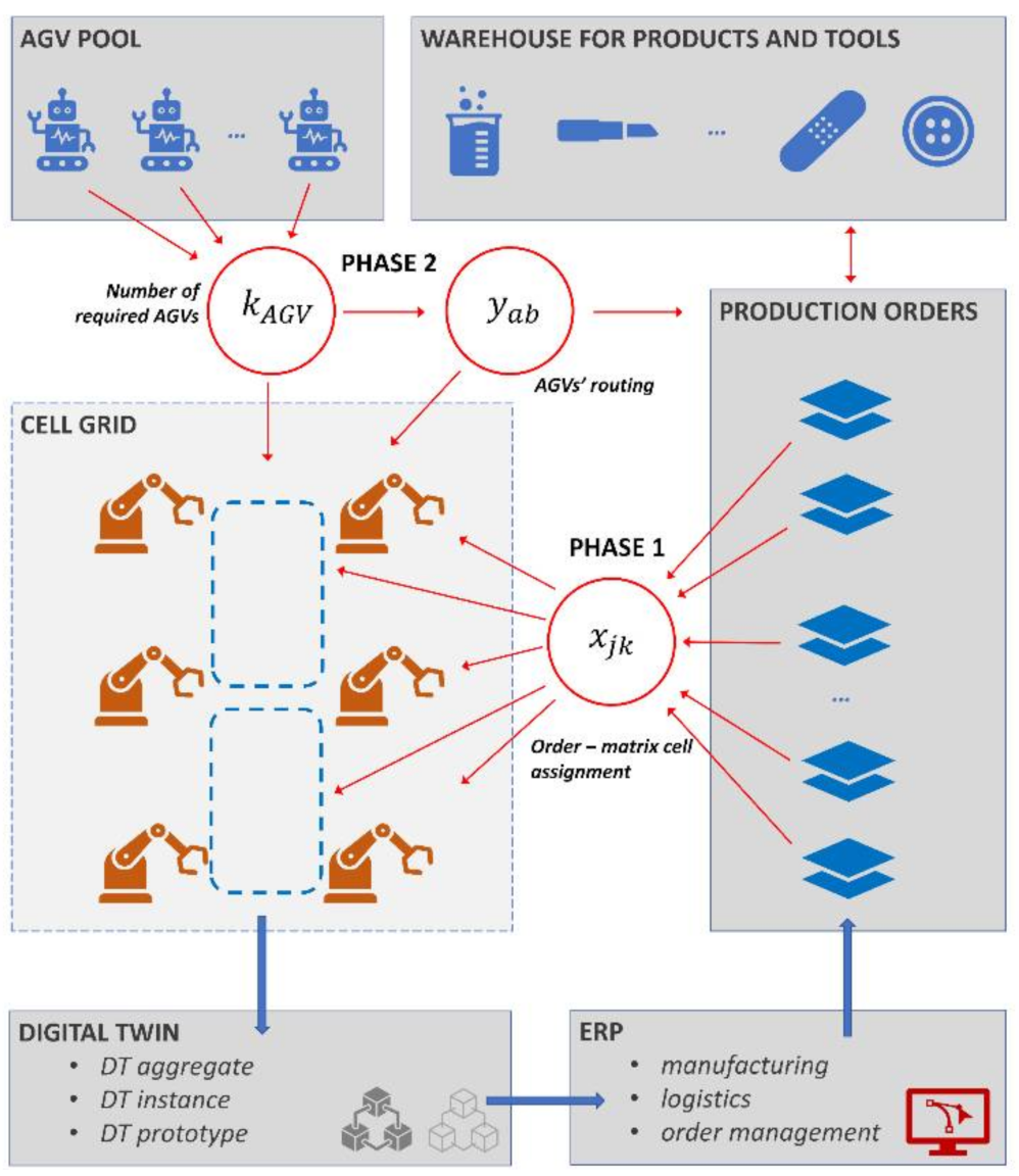
The optimization problem of the matrix production-based in-plant supply has two stages. Within the frame of the first stage, the various production orders must be assigned to the available standardized production cells, while the second phase focuses on the optimal routing of automated guided vehicles. The structure of the integrated assignment and routing model can be seen in
Figure 2.
Phase 1 includes the assignment of production orders to the grid cells. Production orders are generated by the Enterprise Resource Planning (ERP) using the results of Material Requirement Planning (MRP-I) and Manufacturing Resource Planning (MRP-II). The ERP is connected to the sensors and data collection units of cyber-physical environment through a digital twin solution, which makes it possible to make real time analysis, controlling, and forecasting. The size of the AGV pool defines the number of available AGVs, which has a great impact on the in-plant supply process from an availability and efficiency point of view. The more available AGV in the AGV pool, the higher the flexibility and availability, which can influence the utilization of technological resources caused by the changeover time. The second part of the matrix production system includes the storages for tools and components required for the manufacturing. The more the available tool set for required changeover operation, the higher the flexibility and resource utilization for technological resources.
Phase 2 includes the routing of AGVs available in the AGV pool. A typical route of an AGV includes the following tracks: (1) from AGV pool to the warehouse, (2) from the warehouse to the first cell grid of the scheduled route, (3) tracks among cells grids, and (4) from the last cell grid back to the AGV pool. The objective function is either resource- or sustainability-based. Resource-based objective function means the minimization of numbers of required AGVs, while sustainability-based objective means the minimization of energy-consumption of material supply operations. The input parameters of the integrated assignment and routing problem are the followings:
is the changeover time among production orders between production order i and production order k at production cell j, where , and if it is possible to perform a change between production order i and k at production cell j, otherwise ;
3.1. Assignment of Production Operations to Matrix Cells
Within the frame of this phase, the assignment problem of required production operations (production orders) to available standardized flexible production cells is described. The decision variable of the assignment problem is the assignment matrix , which defines that operation production order is assigned to the matrix cell j as kth operation.
The objective function of the first phase of the optimization problem is the minimization of the total operation time within a predefined timeframe, which can be calculated as a sum of the production operations and changeover times:
where
is the production lead time, and
is the changeover time among the various production operations of the standardized production cells. The first part of the objective function represents the total operation time, which can be calculated as follows:
where
is the number of assigned production orders to production cell
j.
The second part of the objective function describes the changeover time among the scheduled operation of matrix cells depending on the assignment:
As an alternative objective function, it is also possible to take into consideration the minimization of the required time spans to fulfil all production orders:
Within the frame of the assignment problem, various constraints must be taken into consideration, like time- and capacity-related constraints. The solution of the assignment problems is limited by these constraints.
Constraint 1 defines that production orders can be assigned to suitable production cells:
Constraint 2 describes that there are production operation pairs and matrix cells, where it is not possible to perform a changeover:
Constraint 3 describes that the operation of production orders must be finished between the lower and upper limit of end time, so it is not allowed to exceed these time-related constraints:
Constraint 4 describes that the number of operations is limited at each production cell, so it is not allowed to exceed the upper limit of operations at a chosen production cell:
Constraint 5 describes that one production order can be assigned exactly to one production cell:
Constraint 6 describes that it is not allowed to exceed the available number of toolsets within a time frame:
3.2. Routing of AGVs in Cell Grid
Within the frame of this phase, the assignment of production orders to matrix cells is given (the production plan is defined) and the optimal routing of available automated guided vehicles must be solved based on the results of the assignment problem. The decision variable of this routing problem is a matrix including permutation arrays, where one permutation array represents the optimal route of an automated guided vehicle. The routing matrix defines that the bth station of AGV a is the matrix cell assigned to production order .
The objective function of the second phase routing problem is the minimization of vehicle fleet size and the minimization of energy consumption of in-plant supply:
where
is the required number of AGVs and
is the calculated energy consumption.
The minimization of the fleet size can be described as the maximum size of fleet within the frame of the time frame:
The minimization of the energy consumption cannot be defined as the minimization of the routes, because energy consumption depends on the weight of the load:
where
is the energy consumption of the AGVs from the warehouse to the first station (matrix cell) of the in-plant supply route,
is the energy consumption of the AGVs among the stations (matrix cells), while
is the energy consumption of the AGVs from the last station (matrix cell) to the warehouse.
The energy consumption of the AGV from the warehouse to the first station (matrix cell) of the in-plant supply route can be defined as a function of length of the route and the weight of the load:
where
is the number of stations of in-plant supply route
a,
is the weight of the load for production order scheduled as station
b of route
a, and
is the length of the transportation between the warehouse and the first matrix cell of the route.
The energy consumption of the AGV among matrix cells can be defined as follows:
where
is the matrix cell ID assigned to the production order, which is scheduled to route
a as station
b.
The energy consumption of the AGV from the last matrix cell of the in-plant supply route and the warehouse can be defined as follows:
where
is the weight of the load for production order scheduled to the last station of in-plant supply route
a, and
is the length of the transportation between the last matrix cell of route
a and the warehouse.
Within the frame of this routing problem, various constraints must be taken into consideration, like time-, capacity- and energy consumption-related constraints. The solution of the routing problem is limited by these constraints.
Constraint 1 defines that it is not allowed to exceed the maximum number of stations within one supply route:
where
is the upper limit of the number of stations assigned to route
a.
In the case of electric AGVs and heavy loadings, it is important to take into consideration the impact of weight and route length on the energy consumption, because in the case of heavy loadings the transportation route can be limited. Energy consumption constraints can be transformed to material flow intensity constraints, because we can define a proportion of energy consumption and material flow intensity (product of length and weight).
Constraint 2 defines that it is not allowed (and not possible) to exceed the material flow intensity, which depends on the weight of loading and length of route:
where
Constraint 3 defines that it is not allowed to exceed the upper and lower limit of arrival time at the matrix cells:
where
is the transportation time between matrix cells assigned to the station
b of route
a, and
is the material handling time (loading and unloading) at matrix cell assigned to the station
d + 1 of route
a. The lower and upper limit for arrival time depends on the assignment matrix.
Constraint 4 defines that it is not allowed to exceed the upper limit of capacity (weight or volume) of automated guided vehicles:
where
is the upper limit of capacity of route (or vehicle)
a.
Constraint 5 defines that supply demands can be transported only with appropriate vehicles:
where
is the set of vehicles appropriate for transportation of required materials and tools of production order
from the warehouse to the assigned matrix cell. The description of nomenclatures used in the mathematical model can be seen in
Appendix A.
To solve the above-described integrated assignment and routing problem, a multiphase optimization algorithm will be described.
4. Results
The multiphase solution algorithm includes the optimization of assignment of production orders to matrix cells and the routing of autonomous guided vehicles among AGV pool, warehouse, and matrix cells. The solution of the assignment problem is based on a black-hole heuristic, while the routing (which also includes a virtual scheduling of production orders) is solved with a flower pollination-based heuristic.
4.1. Black-Hole Heuristic for the Assignment Problem
This population-based heuristic can be summarized in five major steps. The first step is the generation of an initial population of stars representing the initial solutions of the real problem. The coordinates of the generated stars describe the decision variables of the optimization problem. The decision variable of the above-described assignment problem is the assignment matrix, which defines the assignment of production orders to matrix cells, so the initial solutions of the black hole algorithm can be defined as follows:
where
is the ID of the production order assigned to the matrix cell
j as
kth operation of the initial solution
. The initial solution matrix has
m numbers, where
.
, and
is the number of initial solutions.
The second step is the evaluation of the initial solutions with the objective function and calculate the gravity force of the star.
where
is the iteration step and
directly after the initialization of the solution matrix. We can write that
The third phase is to find the best solution in this iteration step. This best solution is dedicated as the black hole of the search space and all other stars representing worst solutions will move toward this solution. We can also define more black holes, but in this case the algorithm is like gravity force algorithm [
57].
The fourth phase of the black hole heuristic is to move the stars towards the black holes. The speed and distance of moving depends on the value of objective function, which is represented by the gravity force of the star.
Stars reaching the event horizon described by the value of Schwarzschild radius will be absorbed and a new star will be initialized. After this step, various termination criteria can be taken into consideration, like computational time or the measure of convergence.
Within the frame of a scenario including 16 production orders and 9 matrix cells, this paper will demonstrate the described model and the results of the black hole heuristic-based assignment optimization. We can define both the availability matrix of matrix cells and the operation time of matrix cells for each production order.
Table 2 shows the operation time of production orders. It is not necessary to describe both matrices, because the operation time can be defined as a ∞ value if the production order cannot be fulfilled in the matrix cell.
We can define the changeover time of matrix cells between production orders. This changeover time is caused by the various required tool sets of production orders. If the production orders are changed at a matrix cell, the following operations are required: (1) take down the used tool set of the matrix cell, (2) collect remaining components of previous production order, (3) transport the old tool set to the tool storage and the remaining components to the warehouse, (4) transport the new required tool set to the next production order from the tool store to the matrix cell, (5) transport the required components from the warehouse to the matrix cell, and (6) set up the new tool set of the production order. These changeover times for this scenario are summarized as a total changeover time in
Table 3.
The time constraints can be defined as the lower and upper limits of the beginning and finishing of production order-related operations.
Table 4 shows the time-based constraints of the scenario. The ∞ value of upper time limit defines that there is no time limit for this production order.
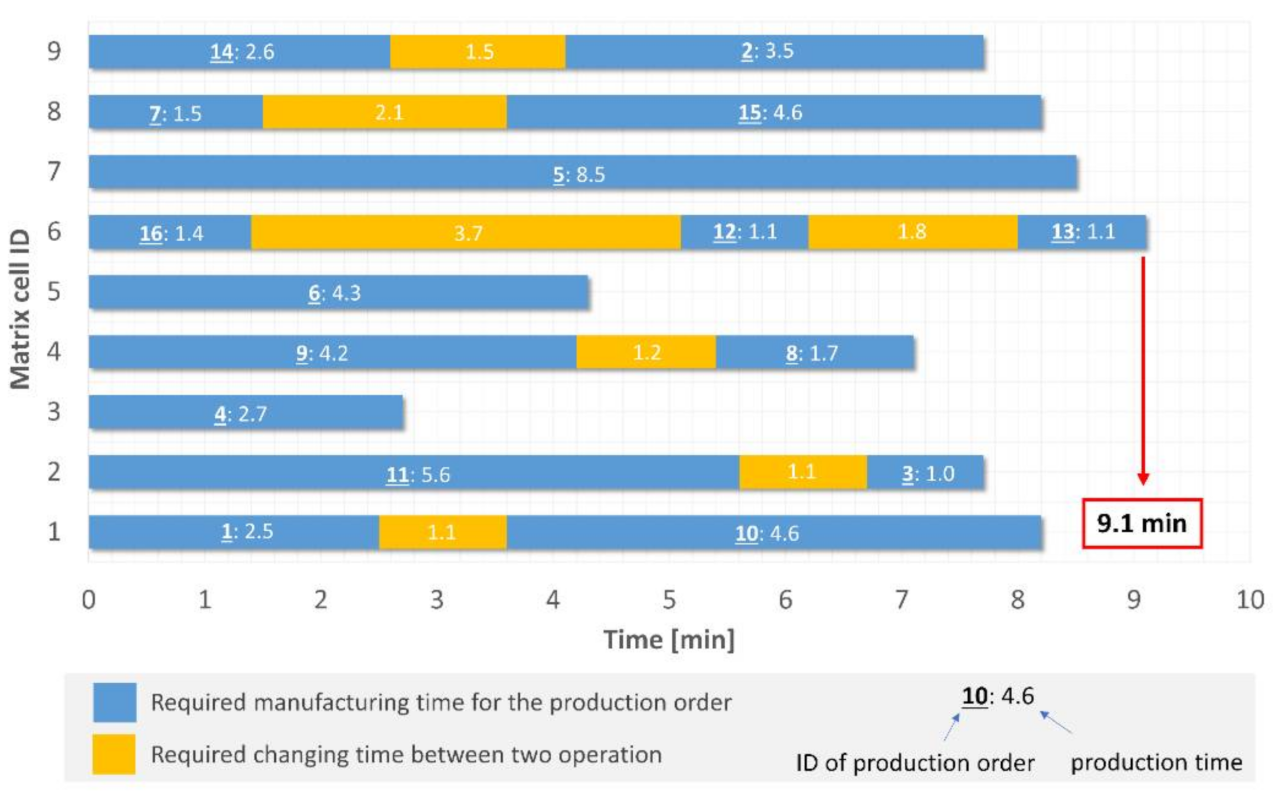
Figure 3 shows the result of the black hole heuristic-based solution algorithm. The value of the objective function is 9.1 min, which means that the last production order will be finished in 9.1 min, which is the cycle time of the 16 production orders. This numerical result shows that the described optimization algorithm can take the time-related constraints into consideration and the algorithm makes it possible to find an optimal solution for the in-plant supply optimization problem. As
Figure 3 shows, in the case of the first scenario the algorithm takes a wide range of the predefined constraints into consideration, including the production time (or lead time) constraint, and the upper and lower limit of beginning and ending time for the production process. At first glance, it may seem that the changeover time in matrix cell 6 could be relocated to the matrix cells 3 or 5, thereby reducing the total manufacturing time, but this is not the case as changeover operations and idle times are not freely moveable due to technological limitations.
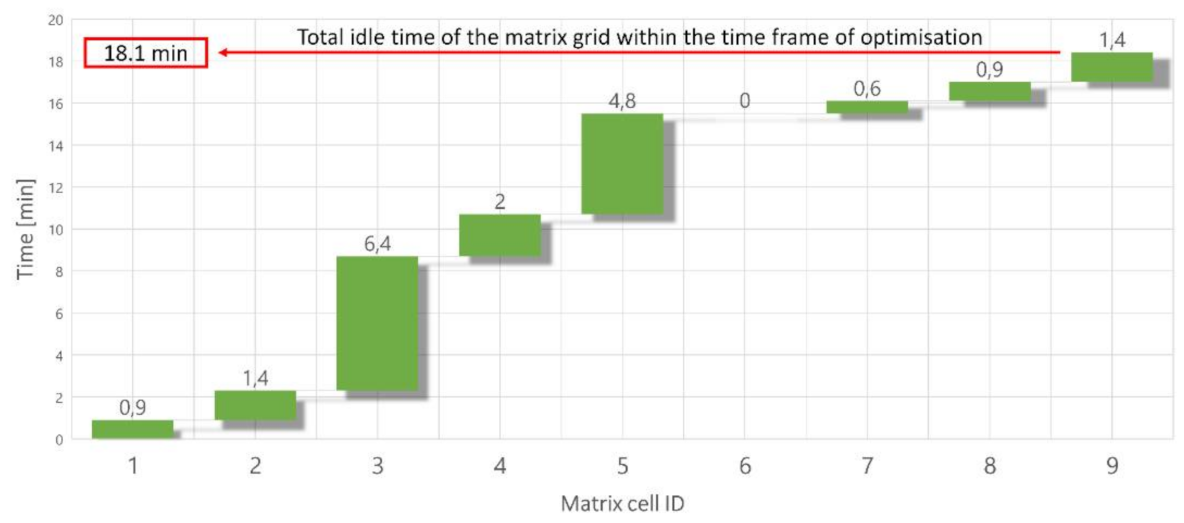
The total idle time of the matrix cells within the time window of the fulfilment of the 16 production demands is 18.4 min. The distribution of the idle time among the matrix cells is shown in
Figure 4.
The technological and logistics resources of the matrix production system are usually state-of-the-art technologies and have expensive operation costs; therefore, it is important to optimize their idle time in order to increase their utilization. In the case of an even distribution of idle time, the production time could be reduced in this case as well, however, as in the case of the changeover time, the time-related constraints and the availability of technological resources do not allow this. The distribution of idle time and the changeover time depends on the flexibility and availability of matrix cells. Higher availability and flexibility makes it possible to produce a wider range of products, which can lead to increased changeover time.
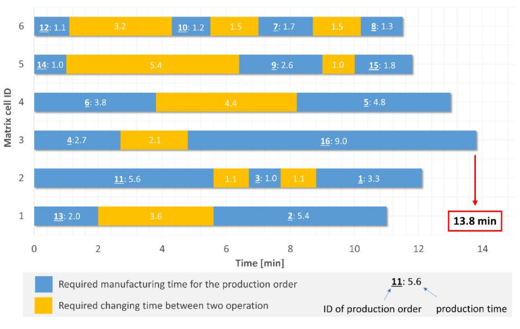
Figure 5 shows the results of a second scenario, where the same operation and changeover times were used, but the number of available matrix cells was reduced to six and the solution was not limited by the time constraints of the previous scenario. The value of the objective function is 13.8 min, which means that the last production order will be finished in 13.8 min. As
Figure 5 shows, the number of available standardized configurable productions or assembly cells has a great impact on the results of in-plant supply processes from a time and capacity point of view. However, in the matrix production system, the processes of technology and logistics are separated, but the decreased number of available technological resources influences the required logistics resources and the computation result shows a higher time span for the working process. In this case, the technological resources must have an increased flexibility and availability for the same manufacturing time. If the availability and flexibility of matrix cells does not increase, the decreased number of technological resources will result in a longer time period being required to complete production, even with a better distribution of idle times.
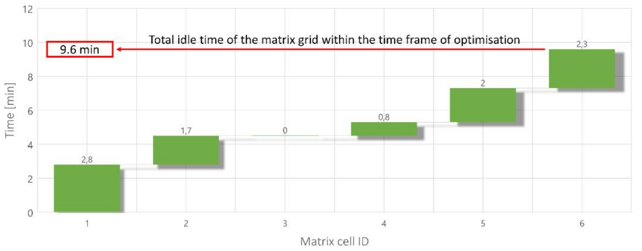
The total idle time of the matrix cells within the time window of the fulfilment of the 16 production demands is 9.6 min. The distribution of the idle time among the matrix cells is shown in
Figure 6. The result shows that the decreased available technological resource influences also the idle time. In this case, the distribution of idle time is more even, but this change in the distribution of idle time has no positive impact on the required manufacturing time because of the decreased number of technological resources.
4.2. Flower Pollination Heuristic for Routing Problem
The first step of the optimization algorithm is the initialization steps, where the basic parameters of the algorithm regarding the real problem and the process of optimization will be defined. The parameters of the real problem are the size and dimension of the search space, as well as the impact of constraints on the search space. The parameters of the algorithm are the followings: switching process between global and local search (biotic and probiotic pollination), termination criteria (computation time, iteration steps, or convergence), and the number of initial solutions (pollen grains).
The second step is the initialization of the solutions, which means the definition of the pollen grains in the search space (pastureland).
where
is the ID of the matrix cell assigned to route
a as
bth station as the initial solution
. The initial solution matrix has
m numbers, where
.
, and
is the number of initial solutions.
The next step is the evaluation of the pollen grains, which is based on the objective function of the routing problem describing the minimization of the energy consumption of the routes defined by solution
in iteration step
:
where
is the iteration step and
directly after the initialization of the solution matrix. We can write that
The third phase is the initialization of a decision number that defines the switch-possibility between biotic and probiotic pollination. The fourth step is the pollination depending on the type of search. In the case of global search, a biotic pollination is performed:
where
is the Levy-distribution.
In the case of local search, an abiotic pollination is performed:
where
and
are random solutions in the iteration step
, and
is a random number between 0 and 1. To transform the continuous representation to a discrete permutation representation, the smallest position value rule was used.
Within the frame of a scenario including 15 production orders and 9 matrix cells, this paper demonstrates the described routing model of the matrix production and the results of the flower pollination-based routing optimization. The optimal assignment of production orders is given, so we can define the lower and upper time limits of production orders, as shown in
Table 5.
The distances among matrix cells, warehouses, and storages are shown in
Table 6.
Figure 7 shows the optimal routing in the matrix grid. There are three routes in the matrix cell within the time span of routing. Six production orders are assigned to route 1 (blue), five production order are assigned to route 2 (red), and three production orders are assigned to route 3 (green). This computational result shows that more AGVs are required in the matrix production system. As presented in the chapter discussing the optimization algorithm, clusters must be formed from the manufacturing tasks. It can be seen in
Figure 7 that the clustering algorithm, when designing the clusters of the production task forming each route, try to form clusters with an even number of production tasks, taking into account the time- and capacity-related constraints. The increased number of available AGVs can lead to decreased cluster, which influences the required manufacturing time and lead time.
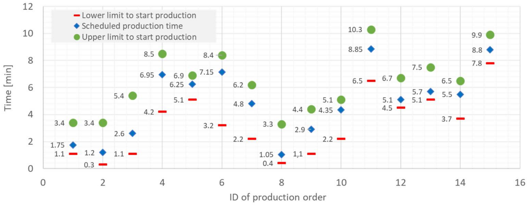
Figure 8 shows the efficiency of the flower pollination-based heuristics. The scheduled production orders are between the predefined lower and upper time limits. The results show that time-related constraints also can be taken into consideration. It is especially important from the production orders point of view, because the predefined time limits, which are based on ERP data, are assumptions of the high service level in matrix production system. The time frame defined by the lower and upper limits influences the solution. In the case of a narrow time frame defined for the manufacturing of production orders, both the availability of technological resources and the availability of logistics resources must be increased to minimize the total required time frame for manufacturing all production orders.
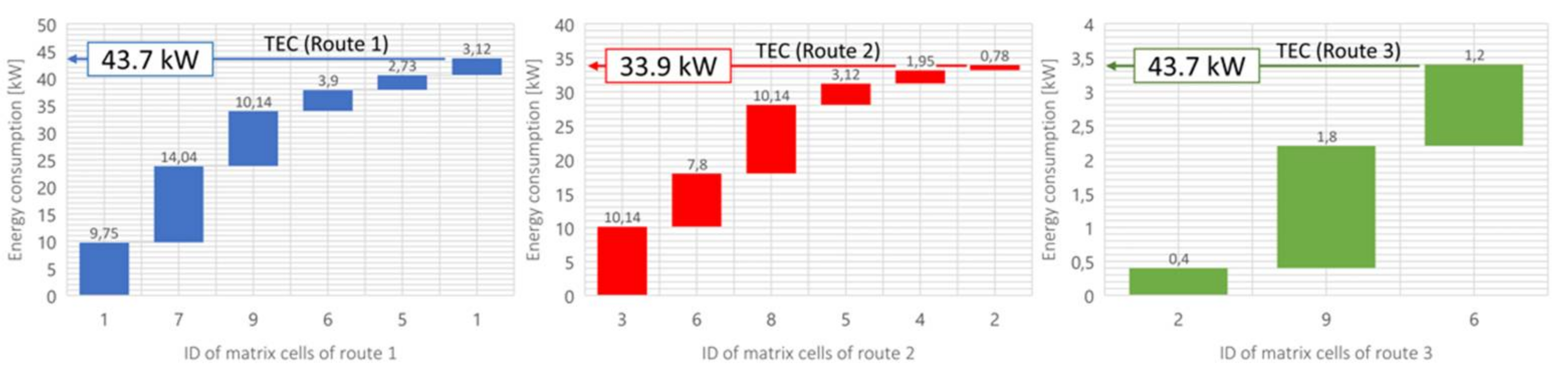
The assignment of production orders to matrix cells and the routing of production orders led to an optimal in-plant supply of matrix cells. The energy consumption, as the objective function of the design problem, can be calculated based on Equation (13) and is shown in
Figure 9. As the computed energy consumption rates show, the energy consumptions of the in-plant supply routes are quasi-uniform, because the state-space of the heuristic optimization model representing the potential solutions of the real problem makes it possible. In the case of a decreased number of AGVs, this uniform distribution is not possible. The energy consumption has a great impact on both the operation cost and on the environmental impact. Depending on the energy generation source (oil, wind, photovoltaic, water, nuclear, biomass, etc.), we can define the emission, and this emission can be taken into consideration as a virtual emission of the manufacturing process. The energy consumption of AGVs influences the required loading of batteries, therefore, the even distribution of energy consumption makes it possible to make a more transparent loading process for the AGVs.
4.3. Challenges and Applicability in Real Industrial Environment
The above-described methodology is applicable in a real industrial environment, but there are challenges that may be faced while applying this proposed model in reality. The application is based on data from the ERP and from the digital twin. The conventional ERP data sets and real-time digital twin-enabled information for simulation-based scenario analysis and forecasting are available using standard interfaces, because standard-based interoperability is an important challenge for large, complex manufacturing systems. The optimization module for in-plant supply design can be implemented either as a part of the ERP or MES, or as an add-on software using standardized channels for information sharing. The implementation cost of these solutions can vary, add-on solutions are cheaper, but ERP-integrated optimization can lead to a more robust and stable solution. The validation of input data for digital twin is also a challenge, because the smart sensor network must have stringent dependability, especially from a reliability and availability point of view, as sensor failures can cause bad data, which influences the results of digital twin-enabled simulation and influences real time decisions. In the case of a conventional manufacturing system, the development of digital twin solutions requires new business models considering expected costs and profit as well as the design, operation, and maintenance requirements. These aspects are summarized in
Figure 10.
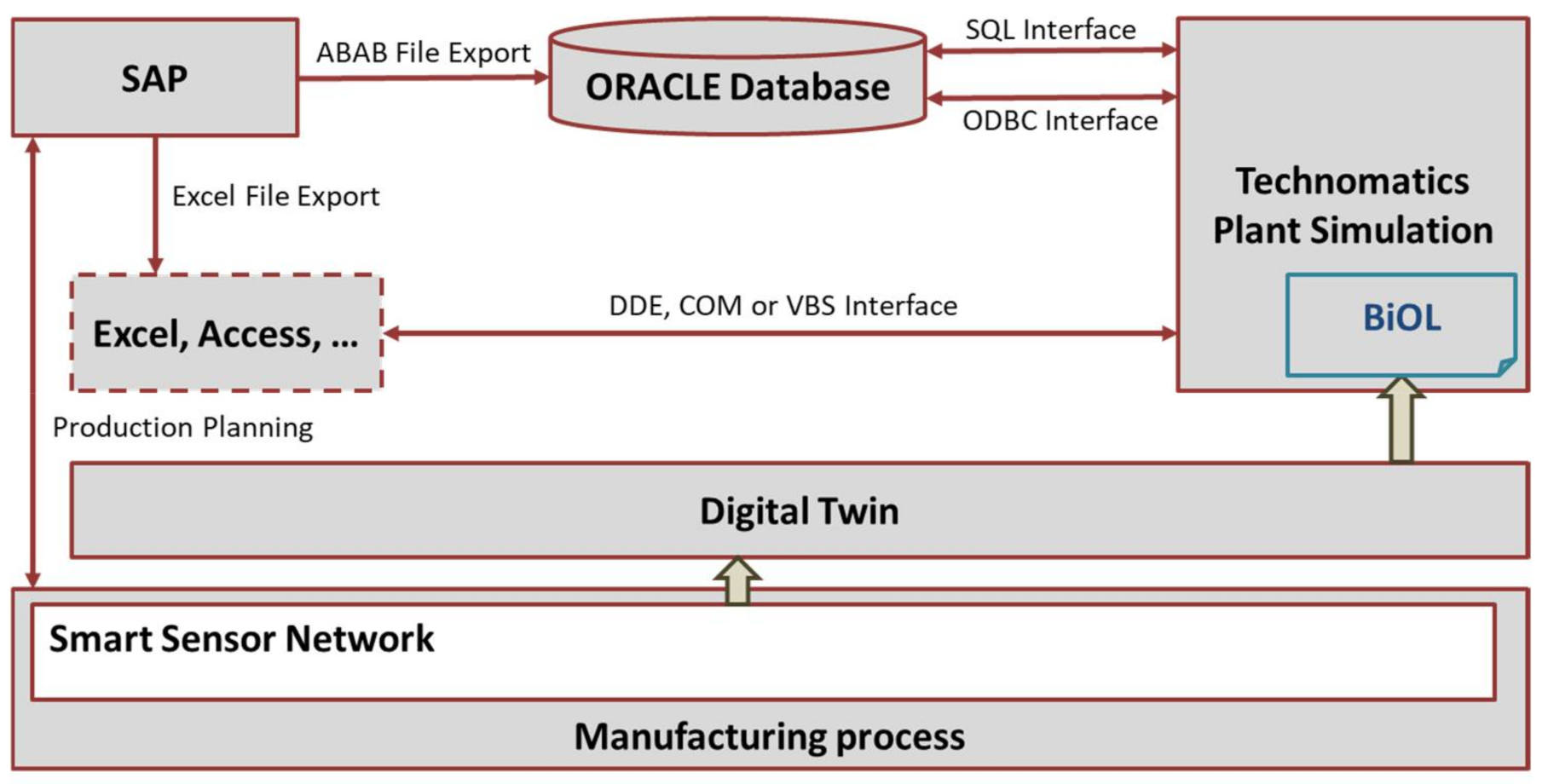
The practical application of the above-described methodology can be performed in many ways, depending on the available IT environment (ERP, sensor networks, simulation software). As an example,
Figure 11 shows a possible solution focusing on the integration of SAP and Technomatix Plant Simulation. Technomatix Plant Simulation is a discrete event simulation software, which makes it possible to use SAP data and integrate real time data from the digital twin of the physical processes in the manufacturing system [
62]. The SAP can generate a data file using Advanced Business Application Programming (ABAB) and this data file can be used by the Technomatix Plant Simulation for scenario analysis, especially in the field of production planning. The transformation of a conventional manufacturing system into a cyber-physical manufacturing system using IoT technologies makes it possible to mirror the physical manufacturing system, and the real time data including failure data and status information from the smart sensor network makes it possible to create a digital twin, which is available for the Technomatix Plant Simulation using ODBC or SQL for Oracle. The SAP data is also available as an Excel file export using Dynamic Data Exchange (DDE), Visual Basic Script (VBS) or Component Object Model (COM). The Technomatix Plant Simulation provides a built-in optimization library (BiOL) for stochastic optimization problems, and it is possible to use this heuristics-enabled solver to perform the proposed optimization tasks.
The above-described scenarios validated the presented in-plant supply model in a cyber-physical production environment and justify the fact that the matrix production, as a new production concept, is suitable for the efficient production of diversified customers’ demands; not only the technology but also the logistic processes must be optimized. In this relation, efficiency means that the matrix production system makes it possible to fulfil diversified customers’ demands near to the efficiency of mass production. KUKA defines this efficiency in the following context: “It (matrix production) will thus become possible to implement the manufacture of customized series as an integral part of Industry 4.0 without limitations in the context of industrial mass production [
12]”. The validation includes the following aspects: (1) the proposed functional model is suitable to support the in-plant supply optimization in a matrix production system; (2) the mathematical model includes time-, capacity-, and energy-related objective functions and constraints, and these objectives have a great impact on the cost-efficiency, availability, performance, energy consumption, and sustainability of the matrix production system; the computational results shows that the optimization algorithm resulted in valid solutions in the matrix production system, where time-, capacity- and energy-related constraints are taken into consideration.
To summarize, the proposed model based on assignment and routing problems of matrix production makes it possible to analyze the impact of assignment of production order to matrix cells and the routing of automated guided vehicles in the matrix grid on the energy efficiency, availability, and required resources of material handling.
As the findings of the literature review show, the articles that addressed the analysis of in-plant supply are focusing on a conventional production environment, but only a few of them aimed to identify the optimization aspects of in-plant supply solutions in matrix production.
The comparison of the results with those from other studies shows that the optimization of material handling processes in cyber-physical systems still need more attention and research. The reason for this is that, in the case of cyber-physical systems, where Industry 4.0 technologies make possible the realization of flexible and efficient operation, the improvement of in-plant supply solutions and the optimization of their processes must be taken into consideration.
5. Discussion and Conclusions
The efficiency of manufacturing systems influences the efficiency of value chains, including purchasing and distribution processes; therefore, it is important to analyze the influencing factors of manufacturing systems and transform them into smart manufacturing systems using IoT technologies [
58,
59,
60]. Within the frame of this research work, the authors developed an integrated model of in-plant supply based on the matrix production concept of KUKA. This model makes it possible to optimize the assignment and routing tasks of this new cyber-physical solution in the era of Industry 4.0. More generally, this paper focused on the mathematical description of the in-plant supply solutions in matrix production, including the assignment of technology and logistics (matrix cells as production resources and production order) and routing of autonomous guided vehicles. Why is so much effort being put into this research? Conventional production environments have been transformed into cyber-physical production, and this new production environment needs more attention both from a technology [
61] and logistics point of view. A comparative table contrasted the proposed methodology in front of related analyzed research works, where the relationship between this solution and past literature was discussed. The existing studies include the optimization of both conventional and cyber-physical manufacturing systems, while only a few of them consider the sustainability-related aspects in matrix production and other cyber-physical manufacturing environments.
The added value of the paper is in the description of the autonomous guided vehicles-based in-plant supply in a cyber-physical environment, where production is based on standardized flexible manufacturing resources. The scientific contribution of this paper for researchers in this field is the mathematical modelling of in-plant supply in cyber-physical production including assignment, routing, and virtually scheduling. The results can be generalized because the model can be applied for different production environments. Managerial decisions can be influenced by the results of this research, because the described method makes it possible to analyze various supply strategies and make decisions regarding the size of AGV pool or strategy of warehousing of components or storage of tools and toolsets for the standardized flexible production cells. This managerial impact results from the fact that the above-mentioned algorithm takes different values of the size of the AGV pool as well as available tools required for changeovers into consideration, and the optimization results show whether or not the in-plant supply process can be performed with the given parameters.
However, there are also limitations of the study and the described model, which provides direction for further research. Within the frame of this model, stochastic parameters were not taken into consideration. In further studies, the model can be extended to a more complex model including Fuzzy sets to describe stochastic processes.


