
A Multi-Model-Particle Filtering-Based Prognostic Approach to Consider Uncertainties in RUL Predictions

Abstract
:1. Introduction
1.1. Prognostic Approaches
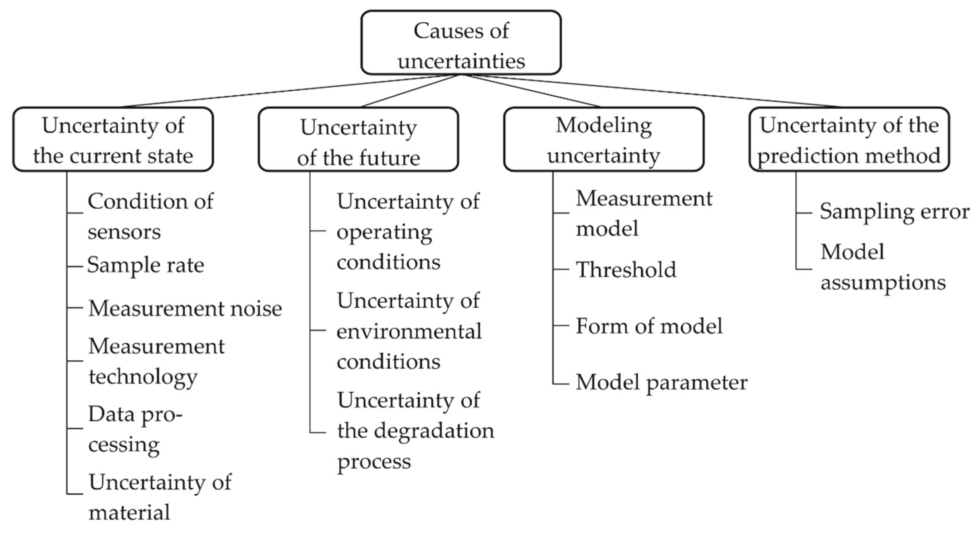
1.2. Uncertainties in Predictions
2. Developing a Prognostic Approach Considering Uncertainties
2.1. General Stochastic Filtering Approaches
2.2. Particle Filter
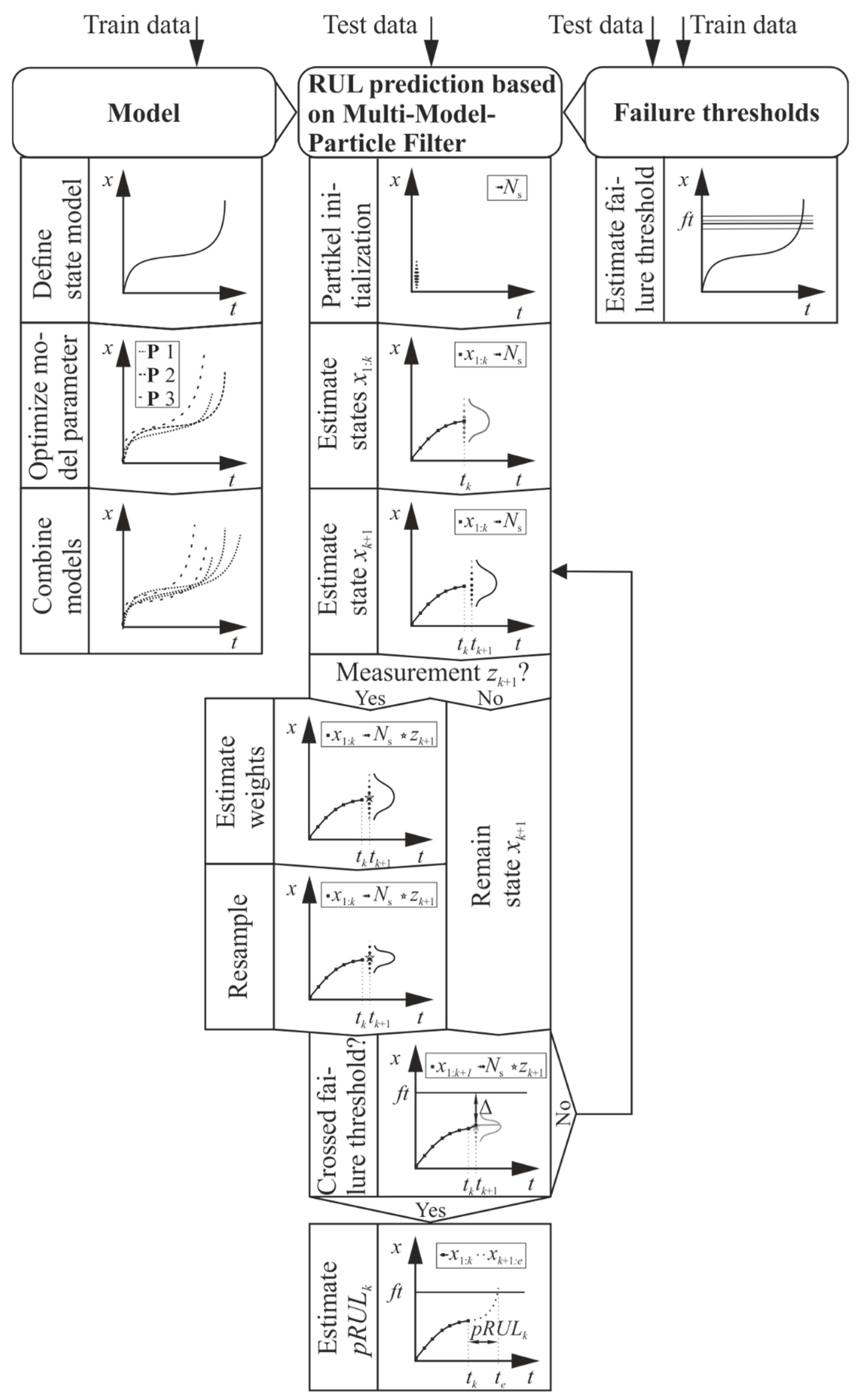
2.3. Multi-Model-Particle Filter
2.4. Estimating Thresholds Considering Uncertainties
2.5. Use Case: Rubber-Metal-Elements
2.5.1. Attributes and Applications
2.5.2. Methods to Approximate Lifetime
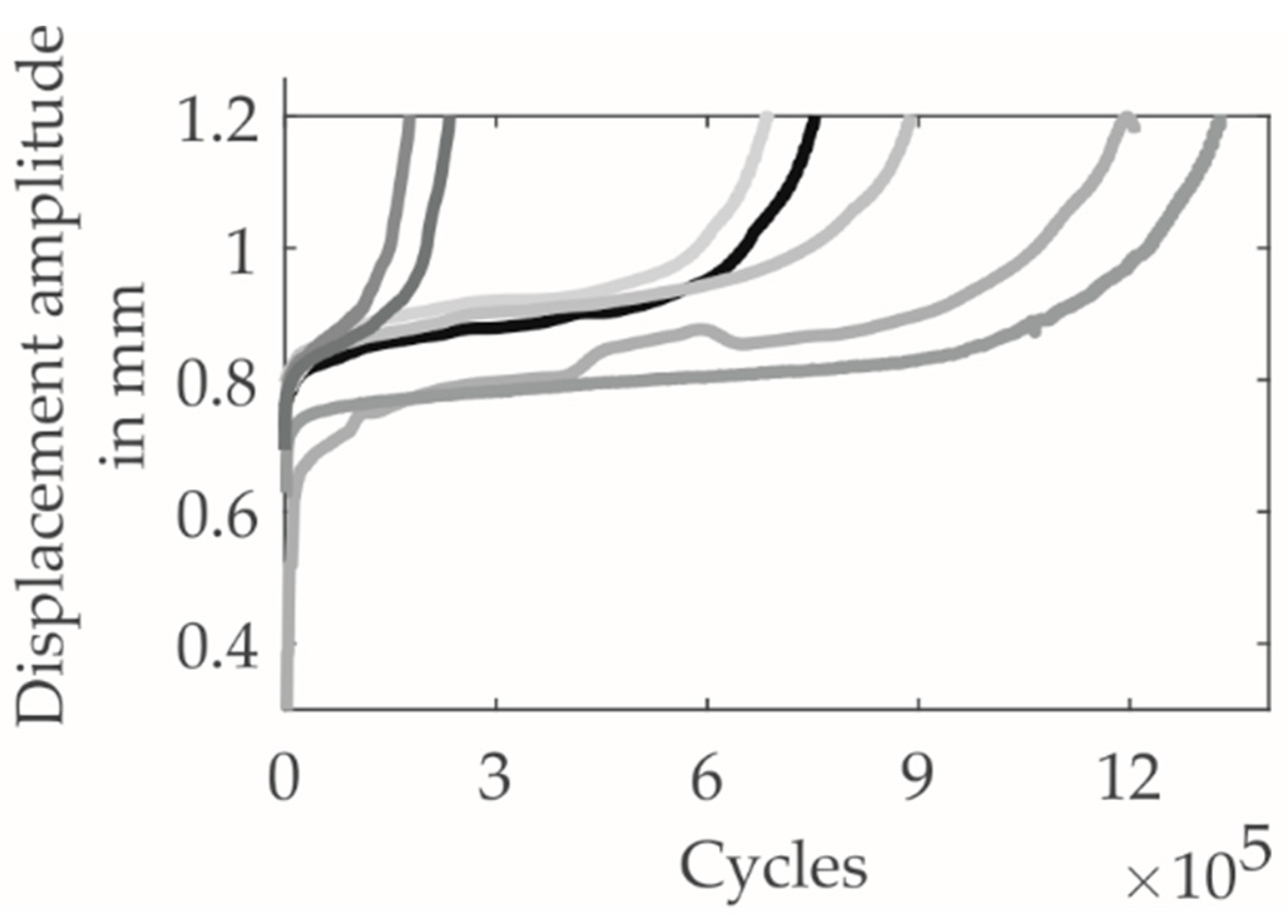
2.5.3. Lifetime Tests
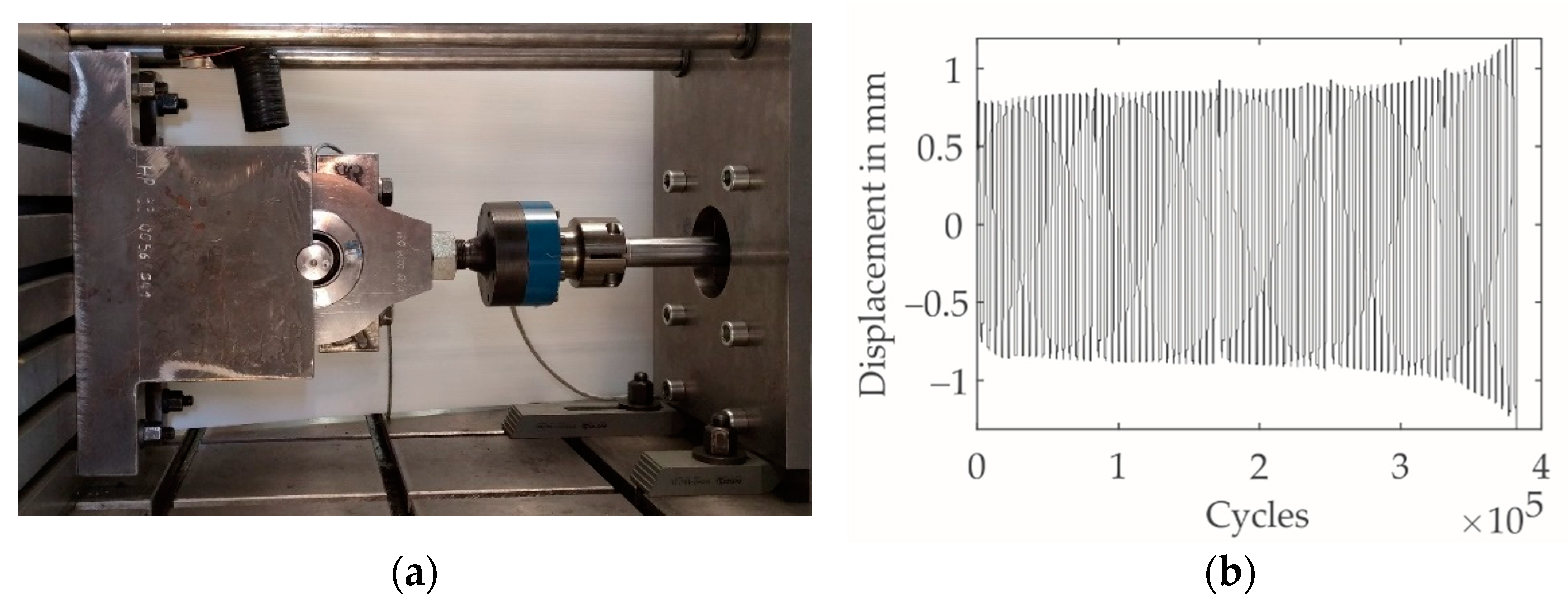
2.5.4. Developing Measurement Concepts
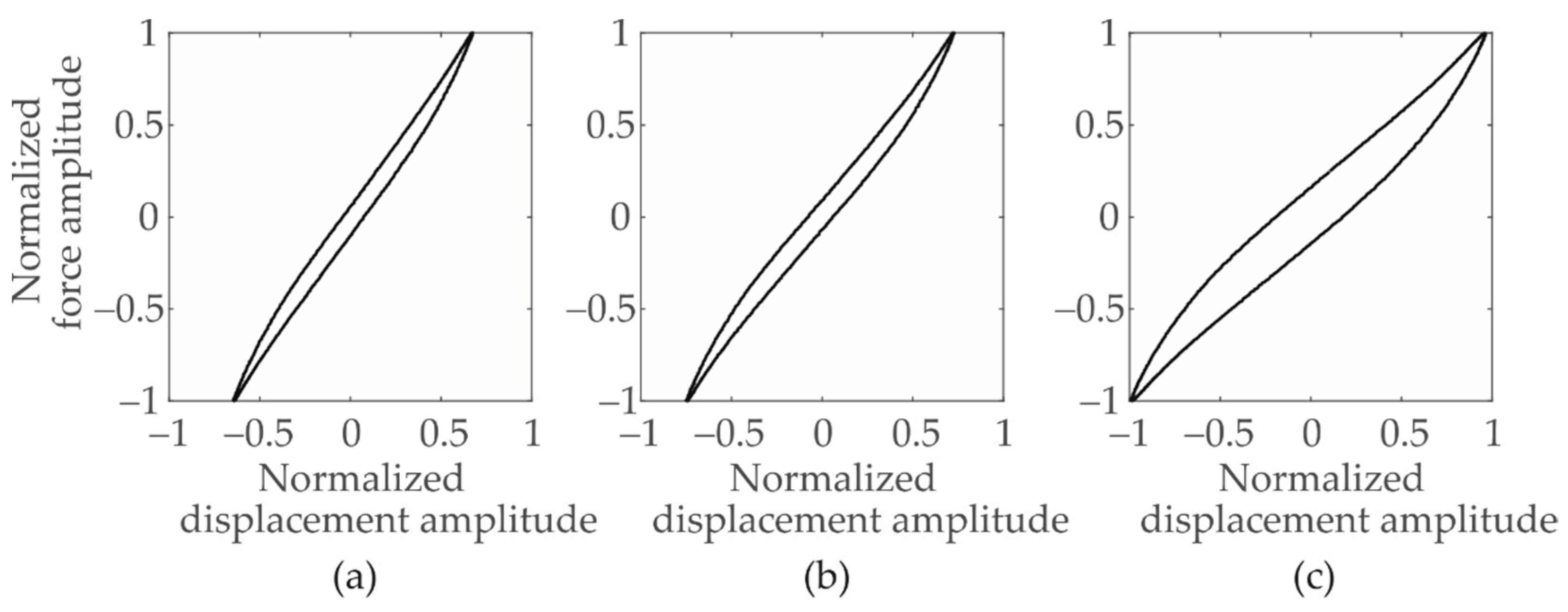
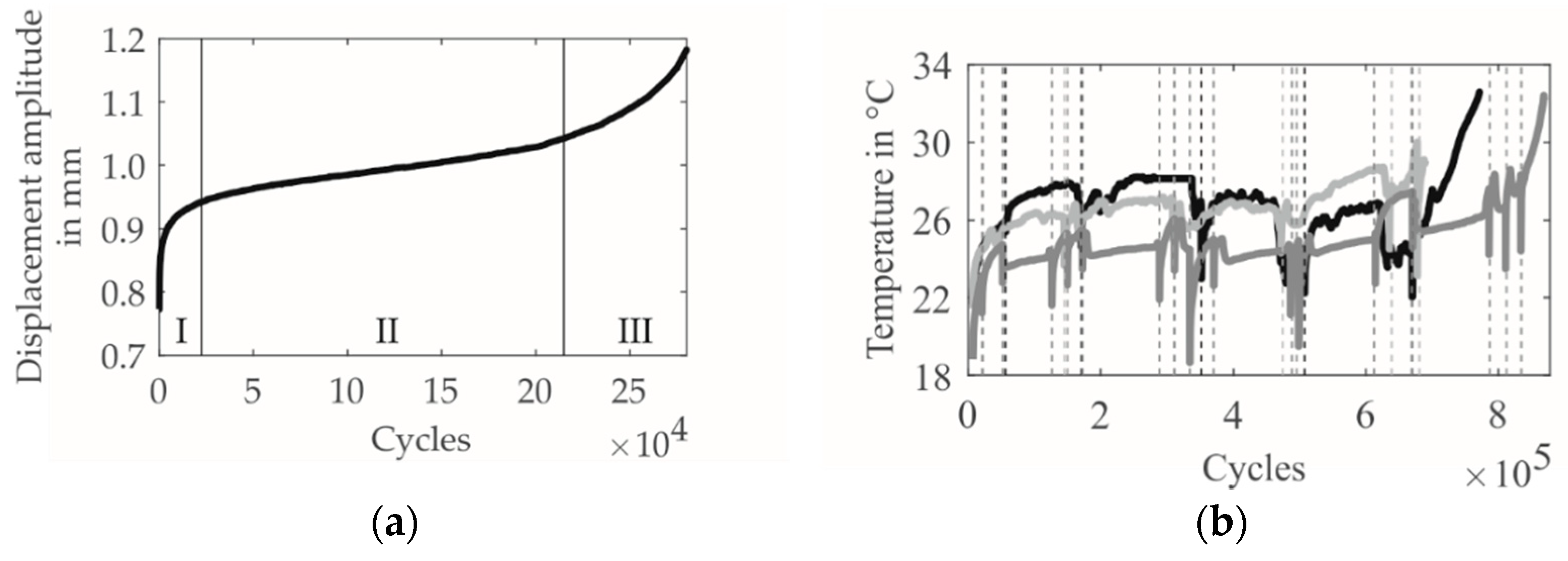
Displacement-Based Concept
Temperature-Based Concept
2.5.5. Preprocessing and Feature Selection
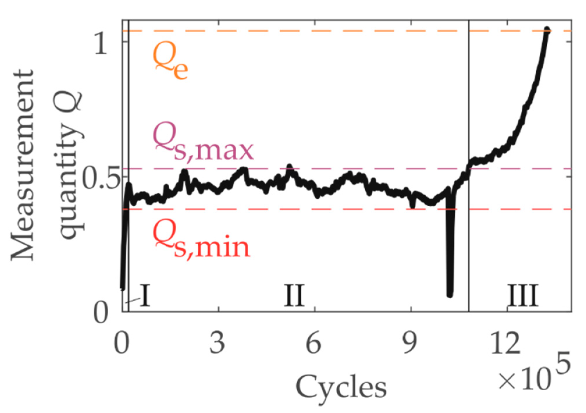
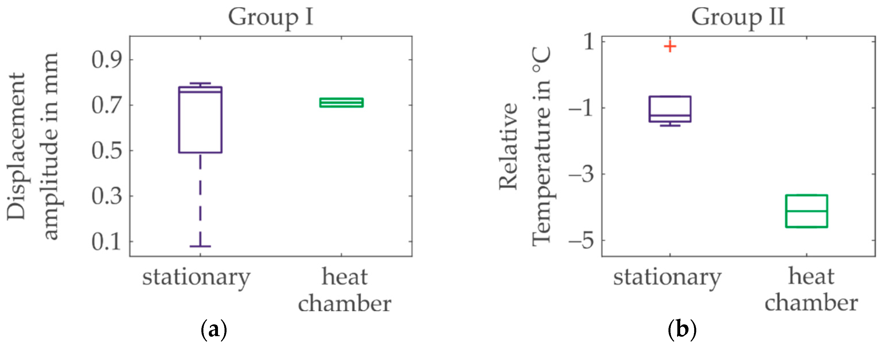
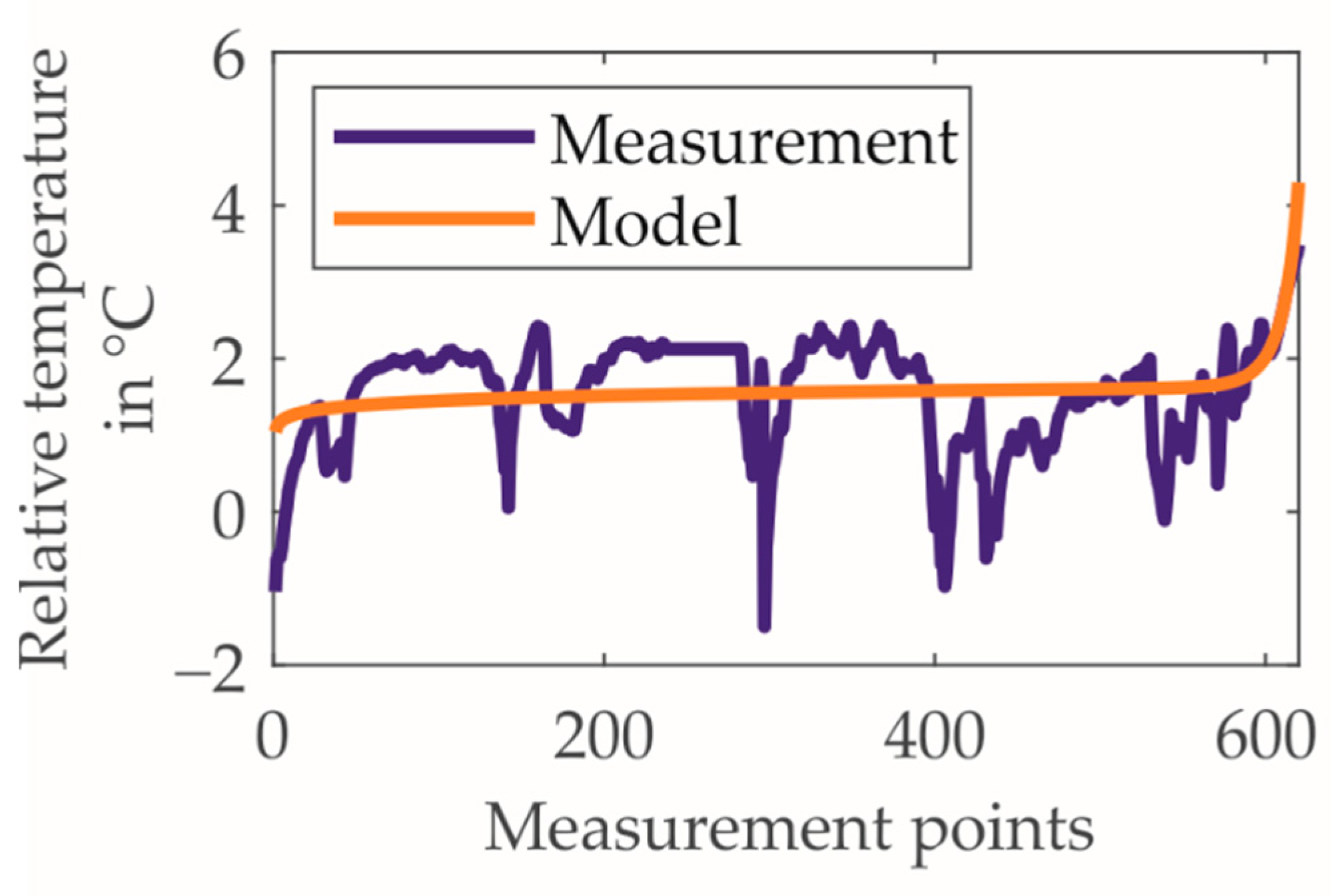
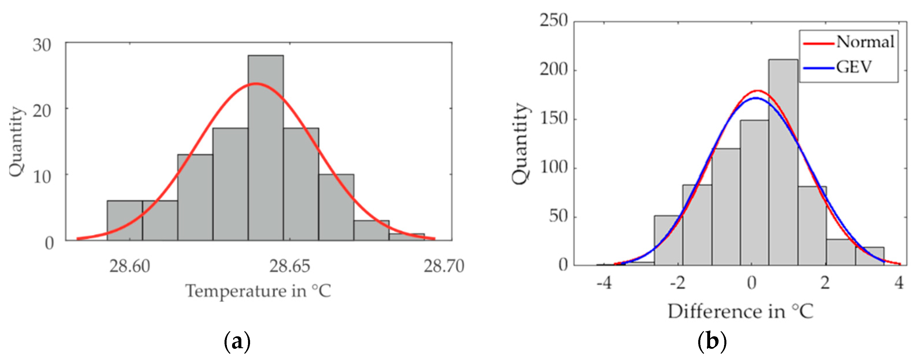
2.5.6. Uncertainty Analysis
3. Evaluation of the Developed Condition Monitoring System of Rubber-Metal-Elements
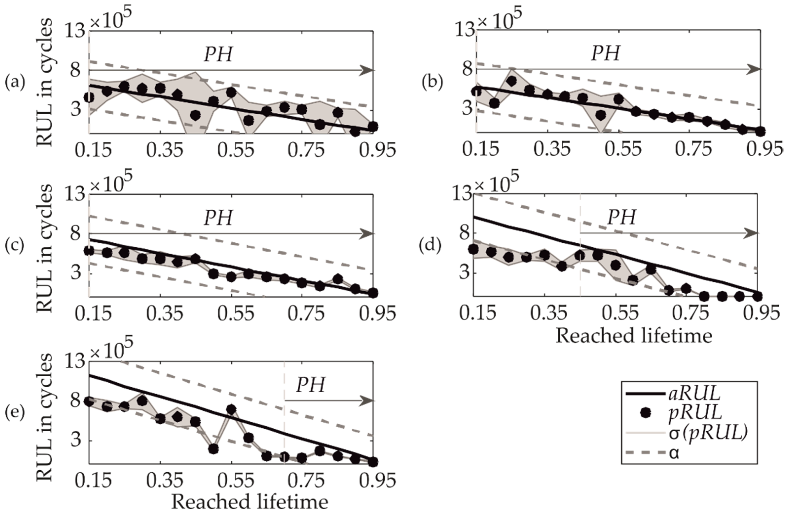
3.1. Predictions of RUL
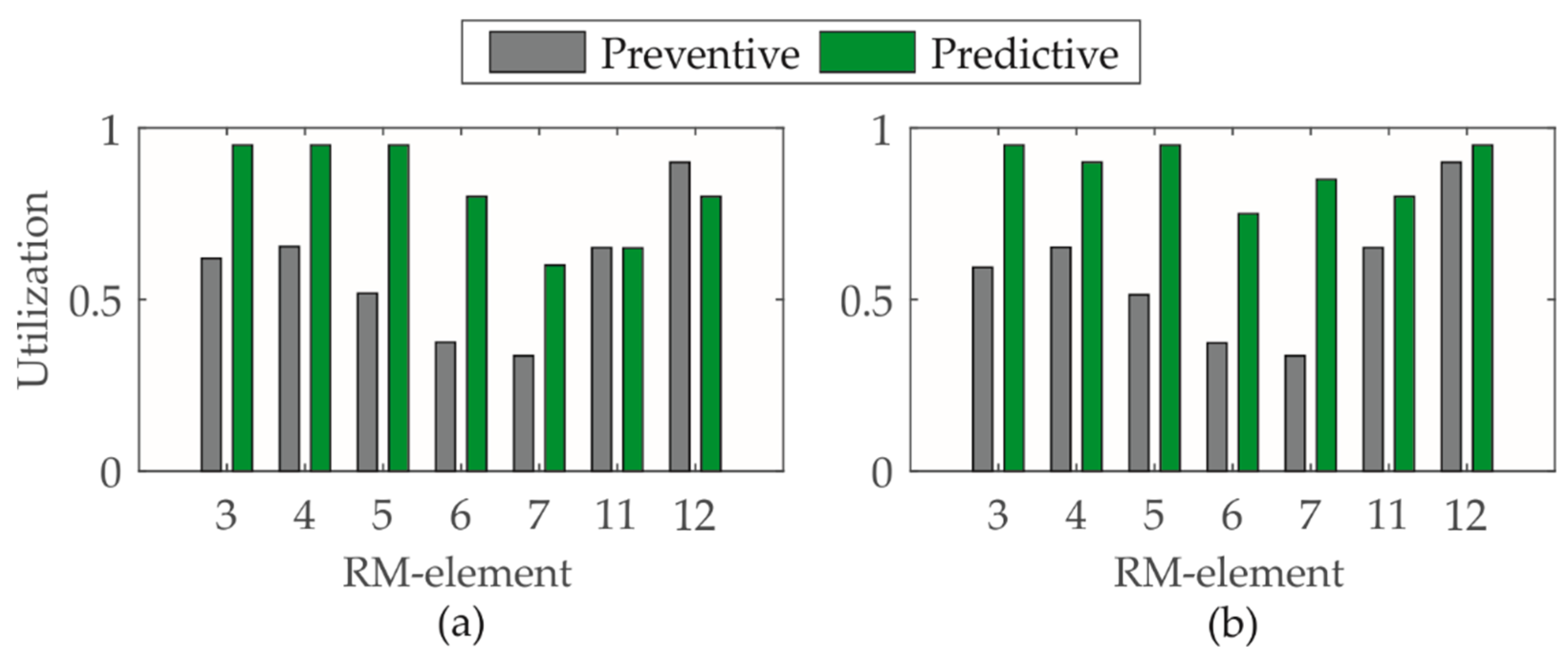
3.2. Comparison of Classical One-Model Particle Filtering-based Prognostic Approach and the Developed Multi-Model-Particle Filtering-based Prognostic Approach
3.3. Discussion
4. Conclusions
Funding
Conflicts of Interest
Appendix A
| Load measurements of the current system z1:c until current time tc |
| Load state model combination or m models |
| Select only models that enable a longer lifetime than time tc: tend(mi)> tc |
| Either define fixed failure threshold ft or estimate adaptive ft (according to Equation (5)) |
| Set parameters of the particle filter based on the measurements and its uncertainty |
| Initialize particles equally over m models (see Equation (4)) |
| Estimate current state xk based on the particles |
| For xk < ft |
| Estimate next state xk+1 (according to Equation (4)) |
| Is tc > tk+1 |
| Estimate (importance) weights for each particle and normalize them |
| Importance resampling of particles and connected models to update next state xk+1 |
| Else |
| xk+1 = xk+1 and use the same models for the next time step k+1 |
| Ek = k + 1 |
| Estimate pRUL based on the time steps k and the current time tc |
References
- DIN ISO 17359. Zustandsüberwachung und—Diagnostik von Maschinen—Allgemeine Anleitungen; Beuth Verlag GmbH: Berlin, Germany, 2017. [Google Scholar]
- Goebel, K.; Saxena, A.; Daigle, M.; Celaya, J.; Roychoudhury, I.; Clements, S. Introduction to Prognostics; PHM Society: Dresden, Deutschland, 2012. [Google Scholar]
- Javed, K.; Gouriveau, R.; Zerhouni, N. State of the Art and Taxonomy of Prognostics Approaches, Trends of Prognostics Applications and open Issues towards Maturity at different Technology Readiness Levels. Mech. Syst. Signal Process. 2017, 94, 214–236. [Google Scholar] [CrossRef]
- DIN ISO 17359. Zustandsüberwachung und—Diagnostik von Maschinen—Allgemeine Anleitungen; Beiblatt 1: Erläuterungen zu Fachbegriffen; Beuth Verlag GmbH: Berlin, Germany, 2017. [Google Scholar]
- Chapman, P.; Clinton, J.; Kerber, R.; Khabaza, T.; Reinartz, T.; Shearer, C.; Wirth, R. CRISP-DM 1.0: Step-by-Step Data Mining Guide. 2020. Available online: https://the-modeling-agency.com/crisp-dm.pdf (accessed on 11 February 2020).
- Touret, T.; Changenet, C.; Ville, F.; Lalmi, M.; Becquerelle, S. On the use of temperature for online condition monitoring of geared systems. Mech. Syst. Signal Process. 2018, 101, 197–210. [Google Scholar] [CrossRef]
- Crabtree, C.J.; Zappalá, D.; Tavner, P.J. Survey of Commercially Available Condition Monitoring Systems for Wind Turbines. 2014. Available online: https://dro.dur.ac.uk/12497/ (accessed on 11 February 2020).
- Lachmann, S. Kontinuierliches Monitoring zur Schädigungsverfolgung an Tragstrukturen von Windenergieanlagen. Ph.D. Thesis, Ruhr-Universität Bochum, Bochum, Germany, 2014. [Google Scholar]
- Lessmeier, C.; Kimotho, J.K.; Zimmer, D.; Sextro, W. Condition Monitoring of Bearing Damage in Electromechanical Drive Systems by Using Motor Current Signals of Electric Motors: A Benchmark Data Set for Data-Driven Classification. In Proceedings of the European Conference of the Prognostics and Health Management Society 2016, Bilbao, Spain, 5–8 July 2016; pp. 1–17. [Google Scholar]
- Márquez, F.P.G.; Tobias, A.M.; Pérz, J.M.P.; Papaelias, M. Condition Monitoring of Wind Turbines: Techniques and methods. Renew. Energy 2012, 46, 169–178. [Google Scholar]
- Vachtsevanos, G.J. Intelligent Fault Diagnosis and Prognosis for Engineering Systems; Wiley: Hoboken, NJ, USA, 2006. [Google Scholar]
- Atamuradov, V.; Medjaher, K.; Dersin, P.; Lamoureux, B.; Zerhouni, N. Prognostics and Health Management for Maintenance Practitioners—Review, Implementation and Tools Evaluation. Int. J. Progn. Health Manag. 2012, 8, 1–31. [Google Scholar]
- Baraldi, P.; di Maio, F.; Zio, E. Particle Filters for Prognostics; PHM Society: Nantes, France, 2014. [Google Scholar]
- Chang, Y.; Fang, H.; Zhang, Y. A new hybrid Method for the Prediction of the Remaining Useful Life of a Lithium-Ion Battery, Appl. Energy 2017, 206, 1564–1578. [Google Scholar]
- Kan, M.S.; Tan, A.C.C.; Mathew, J. A Review on Prognostic Techniques for non-stationary and non-linear Rotating Systems. Mech. Syst. Signal Process. 2015, 62–63, 1–20. [Google Scholar] [CrossRef]
- Uckun, S.; Goebel, K.; Lucas, P.J.F. Standardizing research methods for prognostics. In Proceedings of the International Conference on Prognostics and Health Management, 2008: PHM 2008, Denver, CO, USA, 6–9 October 2008; pp. 1–10. [Google Scholar]
- Jouin, M.; Gouriveau, R.; Hissel, D.; Péra, M.-C.; Zerhouni, N. Particle Filter-Based Prognostics: Review, Discussion and Perspectives. Mech. Syst. Signal Process. 2016, 72–73, 2–31. [Google Scholar] [CrossRef]
- An, D.; Kim, N.H.; Choi, J.-H. Options for prognostics methods: A review of data-driven and physics-based prognostics. In Proceedings of the Annual Conference of the PHM Society, New Orleans, LA, USA, 14–17 October 2013; pp. 1–14. [Google Scholar]
- Guo, L.; Peng, Y.; Liu, D.; Luo, Y. Comparison of resampling algorithms for particle filter based remaining useful life estimation. In Proceedings of the 2015 IEEE Conference on Prognostics and Health Management (PHM), Coronado, CA, USA, 18–24 October 2015; pp. 1–8. [Google Scholar]
- Doucet, A.; Godsill, S.; Andrieu, C. On sequential Monte Carlo sampling methods for Bayesian filtering. Stat. Comput. 2000, 10, 197–208. [Google Scholar] [CrossRef]
- Kimotho, J.K. Development and Performance Evaluation of Prognostic Approaches for Technical Systems; Universitat Paderborn: Paderborn, Germany, 2016. [Google Scholar]
- Wang, J.; Gao, R.X. Multiple model particle filtering for bearing life prognosis. In Proceedings of the 2013 IEEE Conference on Prognostics and Health Management, Gaithersburg, MD, USA, 24–27 June 2013. [Google Scholar]
- Saha, B.; Goebel, K. Modeling li-ion battery capacity depletion in a particle filtering framework. In Proceedings of the Annual Conference of the PHM Society 2009, San Diego, CA, USA, 27 September–1 October 2009; pp. 1–10. [Google Scholar]
- Alonso, J.A.O.; Weihrauch, C.; Bertram, T. A Model-Based Approach for Predicting the Remaining Driving Range in Electric Vehicles. In Proceedings of the Annual Conference of the Prognostics and Health Management Society, New Orleans, LA, USA, 14–17 October 2013. [Google Scholar]
- Caesarendra, W.; Niu, G.; Yang, B.-S. Machine condition prognosis based on sequential Monte Carlo method. Expert Syst. Appl. 2010, 37, 2412–2420. [Google Scholar] [CrossRef]
- Kimotho, J.K.; Meyer, T.; Sextro, W. PEM fuel cell prognostics using particle filter with model parameter adaptation. In Proceedings of the 2014 IEEE Conference on Prognostics and Health Management, Cheney, WA, USA, 22–25 June 2014. [Google Scholar]
- Jouin, M.; Gouriveau, R.; Hissel, D.; Péra, M.-C.; Zerhouni, N. Prognostics of PEM Fuel Cells under a combined Heat and Power Profile. IFAC-PapersOnLine 2015, 48, 26–31. [Google Scholar] [CrossRef]
- Arachchige, B.; Perinpanayagam, S.; Jaras, R. Enhanced Prognostic Model for Lithium Ion Batteries Based on Particle Filter State Transition Model Modification. Appl. Sci. 2017, 7, 1172. [Google Scholar] [CrossRef] [Green Version]
- Laayouj, N.; Jamouli, H. Prognosis of Degradation based on a new dynamic Method for Remaining Useful Life Prediction. J. Qual. Maint. Eng. 2017, 23, 239–255. [Google Scholar] [CrossRef]
- Jimenez, J.J.M.; Schwartz, S.; Vingerhoeds, R.; Grabot, B.; Salaün, M. Towards multi-model approaches to predictive maintenance: A systematic literature survey on diagnostics and prognostics. J. Manuf. Syst. 2020, 56, 539–557. [Google Scholar] [CrossRef]
- Li, P.; Kadirkamanathan, V. Particle filtering based multiple-model approach to fault diagnosis in nonlinear stochastic systems. In Proceedings of the 2001 European Control Conference (ECC), Porto, Portugal, 4–7 September 2001; pp. 1378–1383. [Google Scholar]
- Cadini, F.; Sbarufatti, C.; Corbetta, M.; Giglio, M. A particle filter-based model selection algorithm for fatigue damage identification on aeronautical structures. Struct. Control Health Monit. 2017, 24, e2002. [Google Scholar] [CrossRef]
- Zhang, Z.; Chen, J. Fault detection and diagnosis based on particle filters combined with interactive multiple-model estimation in dynamic process systems. ISA Trans. 2019, 85, 247–261. [Google Scholar] [CrossRef]
- Akca, A.; Efe, M.Ö. Multiple Model Kalman and Particle Filters and Applications: A Survey. IFAC-PapersOnLine 2019, 52, 73–78. [Google Scholar] [CrossRef]
- Kimotho, J.K.; Sondermann-Woelke, C.; Meyer, T.; Sextro, W. Machinery Prognostic Method Based on Multi-Class Support Vector Machines and Hybrid Differential Evolution—Particle Swarm Optimization. Chem. Eng. Trans. 2013, 33, 619–624. [Google Scholar] [CrossRef]
- Chehade, A.; Bonk, S.; Liu, K. Sensory-Based Failure Threshold Estimation for Remaining Useful Life Prediction. IEEE Trans. Reliab. 2017, 66, 939–949. [Google Scholar] [CrossRef]
- Goebel, K.; Daigle, M.; Saxena, A.; Sankararaman, S.; Roychoudhury, I.; Celaya, J. Prognostics: The Science of Prediction, 1st ed.; CreateSpace Independent Publishing Platform: Scotts Valley, CA, USA, 2017. [Google Scholar]
- Koenen, J.F. Ein Beitrag zur Beherrschung von Unsicherheit in Lastmonitoring-Systemen. Ph.D. Thesis, Universität Siegen, Siegen, Germany, 2016. [Google Scholar]
- Baraldi, P.; Popescu, I.C.; Zio, E. Methods of Uncertainty Analysis in Prognostics. 2012. Available online: https://hal-supelec.archives-ouvertes.fr/hal-00609156 (accessed on 11 February 2020).
- Valeti, B.; Pakzad, S.N. Remaining useful life estimation of wind turbine blades under variable wind speed conditions using particle filters. In Proceedings of the Annual Conference of the PHM Society 2018, Philadelphia, PA, USA, 24–27 September 2018; pp. 1–10. [Google Scholar]
- Baraldi, P.; Mangili, F.; Zio, E. Investigation of uncertainty treatment capability of model-based and data-driven prognostic methods using simulated data. Reliab. Eng. Syst. Saf. 2013, 112, 94–108. [Google Scholar] [CrossRef] [Green Version]
- Su, X.; Wang, S.; Pecht, M.; Zhao, L.; Ye, Z. Interacting Multiple Model Particle Filter for Prognostics of Lithium-Ion Batteries. Microelectron. Reliab. 2017, 70, 59–69. [Google Scholar] [CrossRef]
- Sankararaman, S.; Goebel, K. Uncertainty in Prognostics and Systems Health Management, Int. J. Progn. Health Manag. 2015, 6, 1–14. [Google Scholar]
- Usynin, A.; Hines, J.W.; Urmanov, A. Uncertain failure thresholds in cumulative damage models. In Proceedings of the Annual Reliability and Maintainability Symposium, 2008: RAMS 2008, Las Vegas, NV, USA, 28–31 January 2008; pp. 334–340. [Google Scholar]
- Acuña-Ureta, D.E.; Orchard, M.E.; Wheeler, P. Computation of time probability distributions for the occurrence of uncertain future events. Mech. Syst. Signal Process. 2021, 150, 107332. [Google Scholar] [CrossRef]
- Peng, W.; Ye, Z.-S.; Chen, N. Bayesian Deep-Learning-Based Health Prognostics Toward Prognostics Uncertainty. IEEE Trans. Ind. Electron. 2020, 67, 2283–2293. [Google Scholar] [CrossRef]
- Kraemer, P. Schadensdiagnoseverfahren für die Zustandsüberwachung von Offshore-Windenergieanlagen. Ph.D. Thesis, Universität Siegen, Siegen, Germany, 2011. [Google Scholar]
- Sharma, A.; Golubchik, L.; Govindan, R. On the Prevalence of Sensor Faults in Real-World Deployments. In Proceedings of the 4th Annual IEEE Communications Society Conference on Sensor, Mesh and Ad Hoc Communications and Networks, San Diego, CA, USA, 18–21 June 2007; pp. 213–222. [Google Scholar]
- Chen, J.; Ma, C.; Song, D.; Xu, B. Failure Prognosis of multiple uncertainty system based on Kalman filter and its application to aircraft fuel system. Adv. Mech. Eng. 2016, 8, 1–13. [Google Scholar] [CrossRef] [Green Version]
- Corbetta, M.; Sbarufatti, C.; Saxena, A.; Goebel, K. A Bayesian framework for fatigue life prediction of composite laminates under co-existing matrix cracks and delamination. Compos. Struct. 2018, 187, 58–70. [Google Scholar] [CrossRef]
- Tamssaouet, F.; Nguyen, K.T.P.; Medjaher, K.; Orchard, M. A contribution to online system-level prognostics based on adaptive degradation models. In Proceedings of the Fifth European Conference of the PHM Society 2020, virtual, 27–31 July 2020. [Google Scholar]
- Li, Z.; Goebel, K.; Wu, D. Degradation Modeling and Remaining Useful Life Prediction of Aircraft Engines Using Ensemble Learning. J. Eng. Gas Turbines Power 2019, 141, 1–10. [Google Scholar] [CrossRef] [Green Version]
- Nielsen, J.S.; Sorensen, J.D. Bayesian Estimation of Remaining Useful Life for Wind Turbine Blades. Energy 2017, 10, 664. [Google Scholar] [CrossRef] [Green Version]
- Wen, Y.; Wu, J.; Yuan, Y. Multiple-Phase Modeling of Degradation Signal for Condition Monitoring and Remaining Useful Life Prediction. IEEE Trans. Reliab. 2017, 66, 924–938. [Google Scholar] [CrossRef]
- Orchard, M.; Kacprzynski, G.; Goebel, K.; Saha, B.; Vachtsevanos, G. Advances in uncertainty representation and management for particle filtering applied to prognostics. In Proceedings of the 2008 International Conference on Prognostics and Health Management, Denver, CO, USA, 6–9 October 2008; pp. 1–6. [Google Scholar]
- Sankararaman, S. Significance, Interpretation, and Quantification of Uncertainty in Prognostics and Remaining Useful Life Prediction. Mech. Syst. Signal Process. 2015, 52–53, 228–247. [Google Scholar] [CrossRef]
- Arulampalam, M.S.; Maskell, S.; Gordon, N.; Clapp, T. A Tutorial on Particle Filters for Online Nonlinear/Non-Gaussian Bayesian Tracking. IEEE Trans. Signal Process. 2002, 50, 174–188. [Google Scholar] [CrossRef] [Green Version]
- Müller-Gronbach, T.; Novak, E.; Ritter, K. Monte Carlo-Algorithmen; Springer: Berlin/Heidelberg, Germany, 2012. [Google Scholar]
- Papoulis, A.; Pillai, S.U. Probability, Random Variables, and Stochastic Processes, 4th ed.; McGraw-Hill: Boston, MA, USA, 2002. [Google Scholar]
- Seifzadeh, S.; Khaleghi, B.; Karay, F. Soft-data-constrained multi-model particle filter for agile target tracking. In Proceedings of the 16th International Conference on Information Fusion (FUSION), Istanbul, Turkey, 9–12 July 2013; pp. 564–571. [Google Scholar]
- Junyu, Q.; Gryllias, K.; Mauricio, A. Multiple-Model Estimation-based Prognostics for Rotating Machinery. In Proceedings of the European Conference of Prognostics and Health Management 2021, (virtual), Turin, Italy, 28 June–2 July 2021. [Google Scholar]
- de Micheaux, H.L.; Ducottet, C.; Frey, P. Online multi-model particle-filter-based tracking to study bedload transport. In Proceedings of the IEEE International Conference on Image Processing (ICIP 2016), Phoenix, AZ, USA, 25–28 September 2016; pp. 3489–3493. [Google Scholar]
- Bender, A. Zustandsüberwachung zur Prognose der Restlebensdauer von Gummi-Metall-Elementen unter Berücksichtigung systembasierter Unsicherheiten. Ph.D. Thesis, Universität Paderborn, Paderborn, Germany, 2021. [Google Scholar]
- Nystad, B.H.; Gola, G.; Hulsund, J.E. Lifetime models for remaining useful life estimation with randomly distributed failure thresholds. In Proceedings of the European Conference of Prognostics 2012, Dresden, Germany, 3–5 July 2012. [Google Scholar]
- Orchard, M.E.; Vachtsevanos, G.J. A Particle-Filtering Approach for on-line Fault Diagnosis and Failure Prognosis. Trans. Inst. Meas. Control 2009, 31, 221–246. [Google Scholar] [CrossRef]
- Jablonski, A.; Barszcz, T.; Bielecka, M.; Breuhaus, P. Modeling of Probability Distribution Functions for automatic Threshold Calculation in Condition Monitoring Systems. Measurement 2013, 46, 727–738. [Google Scholar] [CrossRef]
- Bender, A.; Schinke, L.; Sextro, W. Remaining useful lifetime prediction based on adaptive failure thresholds. In Proceedings of the 29th European Safety and Reliability Conference, Hannover, Germany, 22–26 September 2019; pp. 1262–1269. [Google Scholar]
- Domininghaus, H.; Elsner, P.; Eyerer, P.; Hirth, T. (Eds.) Kunststoffe: Eigenschaften und Anwendungen, 8th ed.; Springer: Berlin/Heidelberg, Germany, 2012. [Google Scholar]
- Baur, E.; Brinkmann, S.; Osswald, T.A.; Schmachtenberg, E. Saechtling Kunststoff Taschenbuch, 30th ed.; Carl Hanser Verlag: München, Germany, 2007. [Google Scholar]
- Johlitz, M. Zum Alterungsverhalten von Polymeren: Experimentell gestützte, Thermo-Chemomechanische Modellbildung und Numerische Simulation. Habilitation, Universität der Bundeswehr München, München, Germany, 2015. [Google Scholar]
- Molls, M. Experimentelle und Numerische Untersuchung Ein- und Mehrachsig Belasteter Elastomerbuchsen unter Besonderer Berücksichtigung des Reihenfolgeneinflusses. Ph.D. Thesis, Universität Duisburg-Essen, Duisburg-Essen, Germany, 2013. [Google Scholar]
- Mistler, M. Lebensdauerprognose für dynamisch beanspruchte Elastomerbauteile auf Basis der thermo-mechanischen Materialbeanspruchung. Ph.D. Thesis, Universität Duisburg-Essen, Duisburg-Essen, Germany, 2018. [Google Scholar]
- Flamm, M.; Steinweger, T.; Weltin, U. Festigkeitshypothesen in der rechnerischen Lebensdauervorhersage von Elastomeren. KGK Kautschuk Gummi Kunststoffe 2003, 56, 582–586. [Google Scholar]
- DIN 50100. Schwingfestigkeitsversuch—Durchführung und Auswertung von zyklischen Versuchen mit konstanter Amplitude für metallishe Werkstoffproben und Bauteile; Beuth Verlag GmbH: Berlin, Germany, 2016. [Google Scholar]
- Flamm, M.; Steinweger, T.; Weltin, U. Lebensdauerabschätzung auf Basis eines lokalen Konzepts. In Elastomerbauteile: DVM-Tag 2009; Berlin, Germany, 2009; pp. 79–88. [Google Scholar]
- Giese, U. Aufklärung Ermüdungs- und Schädigungsrelevanter Mechanismen bei Dynamisch Belasteten Technischen Gummiwerkstoffen. Schlussbericht des IGF-Vorhabens Nr. 15694N. 2011. Available online: https://www.dikautschuk.de/fileadmin/files/forschung/abschlussbericht_aif_15694n.pdf (accessed on 3 August 2020).
- Bender, A.; Kaul, T.; Sextro, W. Entwicklung eines Condition Monitoring Systems für Gummi-Metall-Elemente. In Wissenschafts- und Industrieforum 2017: Intelligente Technische Systeme, Paderborn; Paderborn, Germany, 2017; pp. 347–358. [Google Scholar]
- Spitz, M. Modellbasierte Lebensdauerprognose für dynamisch beanspruchte Elastomerbauteile. Ph.D. Thesis, Universität Duisburg-Essen, Duisburg Essen, Germany, 2012. [Google Scholar]
- Abraham, F.; Alshuth, T.; Jerrams, S. Ermüdungsbeständigkeit von Elastomeren in Abhängigkeit von der Spannungsamplitude und der Unterspannung. Available online: https://www.dikautschuk.de/fileadmin/files/leseproben/p_0135.pdf (accessed on 6 April 2018).
- Das, S.N.; Chaudhuri, A.R. Estimation of Life of an Elastomeric Component: A Stochastic Model. DSJ 2011, 61, 257–263. [Google Scholar] [CrossRef] [Green Version]
- Ludwig, M. Entwicklung eines Lebensdauer-Vorhersagekonzepts für Elastomerwerkstoffe unter Berücksichtigung der Fehlstellenstatistik. Ph.D. Thesis, Gottfried Wilhelm-Leibniz-Universität Hannover, Hannover, Germany, 2017. [Google Scholar]
- Zarrin-Ghalami, T. Fatigue Life Prediction and Modeling of Elatomeric Components. Ph.D. Thesis, The University of Toledo, Toledo, OH, USA, 2013. [Google Scholar]
- Harbour, R.J.; Fatemi, A.; Mars, W.V. Fatigue Crack Growth of filled Rubber under constant and variable Amplitude Loading Condition. Fat Frac. Eng. Mat. Struct. 2007, 30, 640–652. [Google Scholar] [CrossRef]
- Kroth, T.; Möller, R.; Melz, T.; Dippel, B.; Lion, A. Konzept zur temperaturabhängigen Lebensdauerabschätzung von Elastomerbauteilen. KGK Kautschuk Gummi Kunststoffe 2016, 4, 44–51. [Google Scholar]
- Meyer, R. Konzept zur Lebensdauerabschätzung von Elastomerbauteilen mit Hilfe der FEM und Fuzzy-Logik. In Proceedings of the Elastomerbauteile: DVM-Tag 2009, Berlin, Germany, 22–24 April 2009; pp. 103–112. [Google Scholar]
- Steinweger, T. Lebensdauerberechnung und Lebensdauerprüfung von Elastomerbauteilen unter mehrachsiger dynamischer Belastung. Schlussbericht. 2006. Available online: http://www.cleaner-production.de/fileadmin/assets/bilder/BMBF-Projekte/01RC0137_-_Abschlussbericht.pdf (accessed on 3 August 2020).
- Flamm, M.; Steinweger, T.; Weltin, U. Schadensakkumulation bei Elastomeren. KGK Kautschuk Gummi Kunststoffe 2002, 55, 665–668. [Google Scholar]
- Wortberg, J.; Mistler, M.; Schulze, A. Lifetime Prediction with nonlinear Damage Accumulation based on Material Stressing Part II: Application to Elastomer Couplings. KGK Kautschuk Gummi Kunststoffe 2017, 8, 55–60. [Google Scholar]
- Platt, W. Betriebssicherheit von elastomerbestückten Wellenkupplungen unter besonderer Berücksichtigung der Einsatztemperatur. Ph.D. Thesis, Rheinisch-Westfälische Technische Hochschule Aachen, Aachen, Germany, 1988. [Google Scholar]
- Ziegler, C.; Mehling, V.; Baaser, H.; Häusler, O. Ermüdung und Risswachstum bei Elastomerbauteilen. In Proceedings of the Elastomerbauteile: DVM-Tag 2009, Berlin, Germany, 22–24 April 2009; pp. 121–130. [Google Scholar]
- Bender, A.; Sextro, W.; Reinke, K. Neuartiges Konzept zur Lebensdauerprognose von Gummi-Metall-Elementen. In Proceedings of the VDI-Fachtagung Schwingungen von Windenergieanlagen 2017, Bremen, Germany, 10 October 2017; pp. 49–60. [Google Scholar]
- Hoenig, M.; Hagmeyer, S.; Zeiler, P. Enhancing Remaining Useful Lifetime Prediction by an Advanced Ensemble Method Adapted to the Specific Characteristics of Prognostics and Health Management. In Proceedings of the 29th European Safety and Reliability Conference, Hannover, Germany, 22–26 September 2019; pp. 1155–1162. [Google Scholar]
- Abid, K.; Sayed-Mouchaweh, M.; Cornez, L. Adaptive machine learning approach for fault prognostics based on normal conditions: Application to shaft bearings of wind turbine. In Proceedings of the Annual Conference of the PHM Society 2019, Scottsdale, AZ, USA, 23–26 September 2019. [Google Scholar]


| Feature | Reference |
|---|---|
| Damping work | [71,72,78] |
| Dynamically stored energy | [79] |
| Relative change in length | [80] |
| Crack length | [81] |
| Crack depth | [82] |
| Rate of crack growth | [83] |
| Strain amplitude | [84,85,86] |
| Stiffness | [73,87,88,89] |
| Tear energy | [76,90] |
| RM-Element | Displacement-Based Concept | Temperature-Based Concept | ||||
|---|---|---|---|---|---|---|
| Mean MAPE | Mean Rate of Negative Errors | Mean PH | Mean MAPE | Mean Rate of Negative Errors | Mean PH | |
| 3 | 45.3 | 11/17 | 0.15–0.95 | 14.9 | 5/17 | 0.15–0.95 |
| 4 | 19.9 | 8/17 | 0.15–0.95 | 20.8 | 7/17 | 0.15–0.95 |
| 5 | 22.7 | 4/17 | 0.15–0.95 | 41.4 | 0/17 | 0.45–0.95 |
| 6 | 56.3 | 0/17 | 0.45–0.95 | 66.8 | 0/17 | 0.80–0.95 |
| 7 | 42.6 | 1/17 | 0.70–0.95 | 82.5 | 1/17 | 0.85–0.95 |
| 11 | 53.2 | 0/17 | 0.70–0.95 | 43.9 | 2/17 | 0.75–0.95 |
| 12 | 57.8 | 17/17 | 0.15–0.95 | 26.9 | 16/17 | 0.70–0.95 |
| Mean | 42.5 | 6/17 | 0.35–0.95 | 42.4 | 4/17 | 0.55–0.95 |
| RM-Element | Displacement-Based Concept | Temperature-Based Concept | ||||
|---|---|---|---|---|---|---|
| Mean MAPE | Mean Rate of Negative Errors | Mean PH | Mean MAPE | Mean Rate of Negative Errors | Mean PH | |
| 3 | 66.9 | 10/17 | 0.40–0.95 | 157.5 | 14/17 | 0.60–0.95 |
| 4 | 44.7 | 11/17 | 0.30–0.95 | 127.4 | 14/17 | 0.50–0.95 |
| 5 | 43.9 | 5/17 | 0.45–0.95 | 79.5 | 7/17 | 0.30–0.95 |
| 6 | 49.3 | 3/17 | 0.60–0.95 | 66.3 | 3/17 | 0.50–0.95 |
| 7 | 79.0 | 0/17 | 0.65–0.95 | 83.3 | 0/17 | 0.60–0.95 |
| 11 | 43.2 | 2/17 | 0.80–0.95 | 44.7 | 0/17 | 0.55–0.95 |
| 12 | 27.2 | 16/17 | 0.70–0.95 | 50.6 | 17/17 | 0.15–0.95 |
| Mean | 50.6 | 7/17 | 0.55–0.95 | 87.1 | 8/17 | 0.45–0.95 |
Publisher’s Note: MDPI stays neutral with regard to jurisdictional claims in published maps and institutional affiliations. |
© 2021 by the author. Licensee MDPI, Basel, Switzerland. This article is an open access article distributed under the terms and conditions of the Creative Commons Attribution (CC BY) license (https://creativecommons.org/licenses/by/4.0/).
Share and Cite
Bender, A. A Multi-Model-Particle Filtering-Based Prognostic Approach to Consider Uncertainties in RUL Predictions. Machines 2021, 9, 210. https://doi.org/10.3390/machines9100210
Bender A. A Multi-Model-Particle Filtering-Based Prognostic Approach to Consider Uncertainties in RUL Predictions. Machines. 2021; 9(10):210. https://doi.org/10.3390/machines9100210
Chicago/Turabian StyleBender, Amelie. 2021. "A Multi-Model-Particle Filtering-Based Prognostic Approach to Consider Uncertainties in RUL Predictions" Machines 9, no. 10: 210. https://doi.org/10.3390/machines9100210
APA StyleBender, A. (2021). A Multi-Model-Particle Filtering-Based Prognostic Approach to Consider Uncertainties in RUL Predictions. Machines, 9(10), 210. https://doi.org/10.3390/machines9100210