Disturbance Simulation in the Packaging Process of Confectionary Using Virtual Commissioning

Abstract

Operator assistance systems can help to reduce disturbance-related machine downtime in food production and packaging processes, especially when combined with machine learning algorithms. These assistance systems analyze the available sensor signals of the process control over time to help operators identify the causes of disturbances. Training such systems requires sufficient test data, which often are hardly available. Thus, this paper presents a study to investigate how test data for teaching machine learning algorithms can be generated by numerical simulation. The potential of using virtual commissioning (VC) software for simulating disturbances of discrete processes is examined, considering the example of a friction and collision-afflicted sub-process from an intermitting wrapping machine for confectionary. In this study the software industrialPhysics (iP) is analyzed regarding accuracy of static and dynamic friction and restitution. The values are verified by setting up virtual substitute tests and comparing the results with analytically determined values. Subsequently, prerecorded disturbances are classified, and seven selected elements are simulated in VC software, recording visual effects and switching the characteristics of sensors. The verification shows that VC software is generally adequate for the assigned task. Restrictions occur regarding the computing power required of the built-in physics engine and the resulting reduction of the machine to be simulated.

1. Introduction

Food production and packaging processes are strongly affected by volatile properties of the processed biogenic materials and the complex behavior of flexible packaging materials. Combined with the complexity of discrete processes themselves, those properties cause disturbances of the process line [1]. To minimize the disturbance, related downtime process control needs to be improved; for example, by enhancing the human–machine interaction with interactive assistance systems, helping to combine different sources of knowledge. A framework for solidly designed interactive assistance systems was for instance proposed by Wandke in 2005 [2]. According to Allais et al. the process-relevant sources of knowledge can be represented by using three different kinds of models: models for human expertise, models for data or physical models [3]. The integration of these models into specific assistance systems for food processing have already been pursued in several, mostly scientific approaches; e.g., for processing of dairy (as proposed by Perrot et al. [4]) or baking products (as presented by Edoura-Gaena et al. and Kansou et al. [5,6]). As stated by Klaeger et al. assistance systems can also improve human decision-making in cases of process disturbances by helping people to understand the root causes of disturbances and therewith to remedy disturbances sustainably [7]. Different root causes of disturbances can furthermore lead to distinctive, temporal switching characteristics of sensors, if they are affected by the specific disturbance, which means that during normal operation the recorded data of the sensor system show a characteristic course over time [7]. Deviations from that course can indicate the causes of a disturbance. Once connected to a database, machine learning algorithms could use these characteristics for detection and differentiation to suggest the most likely root causes of the specific disturbance for the operator’s troubleshooting. Therefore, the measurement data recorded by multiple sensors within the process are combined by special algorithms to improve the operator’s process-monitoring capabilities. This approach of implementing such multi-sensor process-monitoring systems and data processing technologies is already being researched much, in the field of manufacturing systems, for example [8].

To achieve a good performance of the operator assistance system, initial training of the machine learning algorithms is conducted. This requires sensor data to be recorded at the machine and then preprocessed as a feature matrix. For supervised machine learning to classify disturbances, labelled data additionally needs to be made available [9], which needs to contain data about nominal production or information about the current disturbance. For discrete processes, generating these data implicate the following challenges: Due to the complex interactions between volatile product properties and environmental influences, a ground truth of the recorded nominal data cannot be defined [10,11]. They contain statistical deviations over time, the altitude of which depends on the process under consideration [12]. Furthermore, packaging processes are predominantly fast running processes, which is why particular attention must be paid to the correct time synchronization of the disturbances recorded by the operator and the raw senor data [11]. Finally, packaging machines are special-purpose machines designed for a specific task and product range [10], which limits the transferability of an assistance system from one machine to another. Therefore, the learning process of such assistance systems can benefit from the use of simulation tools to generate artificial process and sensor data.

For discrete processing, virtual commissioning (VC) software can theoretically be used to simulate switching characteristics influenced by simulated process disturbances. VC software is already in use to verify the control code of new machinery and installations to shorten their development process [13]. Furthermore, there are many approaches being researched to use VC software during the entire life cycle of a machine. One of these approaches focuses on the connection of virtual reality technology to VC software, enabling several new applications during the commissioning and production phase (for example, customer presentations, operator training, safety validation and hybrid system analysis) [14,15]. Another use case under investigation is the parallel simulation of operation, which can be used for production planning or process control [14,16]. A third approach investigates whether VC software can additionally support the reconditioning process of old machines [17]. However, none of these approaches focus on the process disturbances and their effect on sensor data within a VC model.

Therefore, this paper specifically addresses the machine models built within VC software. In this context, the modelling depth of machines varies greatly depending on the requirements of the simulation [18]. To describe the kinematic and physical behavior of a discrete process, a detailed process model is required [19]. Available VC software uses physics engines to calculate the interaction between the model’s objects, considering the kinematic and physical behavior of rigid bodies [20]. A physics engine is computer software that, in the context described, enables the modelling of a free material flow within the simulation, taking the geometry of the objects; physical properties, such as the masses of the objects and their centers of gravity; and parameters such as friction and restitution into account [21]. Boeing et al. compared the performances and accuracies of different physics engines by using basic scenarios, such as the bouncing of a ball [22]. Hummel et al. extended this comparison by testing the collision and friction behavior of the engines, using scenarios that are more complex [23]. Within their study the collision and friction behavior of the engines was tested by screwing a screw into a nut and the contact behavior by pushing a slider at constant force against a module, fixed within a shaft. Both studies show an overall sufficient physical behavior of the different engines in computer game and aviation applications respectively. Depending on the scenarios, the performances of the different engines vary widely.

A commonly used engine is BulletPhysics, which is a free and open-source software library for multibody simulation (MBS). Its main advantage consists of the capability of calculating simple systems in real-time, which is why this library seems to be very suitable for the VC of packaging machines and equipment for processing piece goods. Within the engine, rigid bodies are represented by triangulated surfaces (see Figure 1).

The mass parameters and the inertia tensor are deduced from the triangulated surfacess of the bodies and the specification of the density. By numerical integration of the density over the surface’s constrained volume, the body’s mass is derived. Afterwards, the inertia tensor is derived by numerical integration of the quadratic distance from each surface point to the center of gravity over the surface’s constrained volume multiplied with the density value.

Rigid body contacts are identified by applying a virtual convex hull around the bodies and calculating their distance by using the Gilbert–Johnson–Keerthi-algorithm. The performance of this library is achieved by using an impact-based approach for simulating rigid body interactions in association with the semi-implicit-Euler-integrator for solving the dynamic system equations [25]. Certainly, the impact-based contact approach and the used integrators are conducive with regard to the simulation speed, but not to the accuracy, which cannot be compared to simulation applications like the finite element method (FEM). Common approaches for rising this accuracy, e.g., reducing the simulation step size or avoiding numerical damping, are not applicable. Besides the accuracies of the engines used, real-time calculation of VC software is also limited to a few, geometrically simple, rigid bodies (e.g., cuboid, sphere) [26]. Objects that are more complex take longer to be calculated [20]. This represents a particular challenge for simulating packaging processes, since they often involve fast-running machines and a high output of geometrically complex products. In addition, other aspects restrict the use of VC software based on these engines to simulate packaging processes: VC software is not able to model complex motions of machine parts, such as the cam mechanism [20]. It is also limited to a rigid body simulation, which restricts the modelling of certain process steps, such as cutting or forming to a black box model. Products like fluids or paper cannot be modeled within the software at all [27].

In conclusion, this paper aims to answer two main questions in order to determine whether VC software has the ability to generate suitable test data for machine learning algorithms and hence shortens learning times by addressing the aforementioned challenges regarding the test data of discrete processes:

• With what accuracy can VC software simulate process disturbances?
• Is the accuracy achieved sufficient to depict the effect of real operational machine behavior?

The accuracy is tested by creating and verifying a model within the VC software, calculating the model error and proposing the evaluation of the simulation results. The second question is addressed by a model analysis simulating normal and disturbed machine operation. The resulting deviations in the process simulation and switching characteristic of the sensor lead to a statement about the applicability of VC software for the assigned task.

2. Materials and Methods

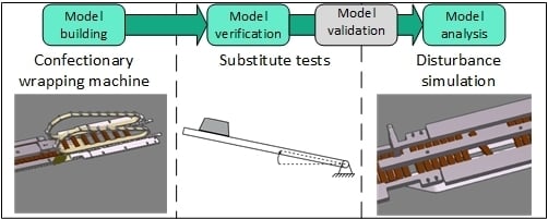
2.1. Preliminary Remark on the Applied Method

Within the simulation study, the steps model building, verification and model analysis were conducted as described in [28]. The first step includes the abstraction and implementation of the machine system in the simulation software used, in such a way that the aforementioned questions of the simulation study can be answered. Within the verification, the correct implementation of the model and its physical behavior are examined. Subsequently, the model analysis was conducted by varying the input parameters of the model to simulate different scenarios. The model can be used to improve the understanding of a process or to generate data about the process. Due to its high effort involved in on-site production, the validation of the model was skipped initially, and the model parameters (e.g., friction coefficients) were estimated based on empirical values. The great experimental effort made to determine these model parameters was based on the many complex interactions of volatile product properties and environmental influences that occur in relation to the process (for example, product dimensions, ambient temperature and the properties of the processed biogenic materials). Nevertheless, to ensure that the process is shown correctly within the simulation, the simulated process was visually compared to the process on the real machine. By specifically varying the empirical parameter values within the model analysis, the simulated machine process and therewith the recorded sensor data over time are affected. Thus, the potential of the VC software to simulate changes within the switching characteristics of sensors resulting from process disturbances is investigated by comparing the recorded data of disturbances to data of the undisturbed process.

2.2. Model Building of the Feeding System of a Wrapping Machine

The disturbance simulation is exemplarily carried out on a virtual model of the feeding system of an intermitting wrapping machine for confectionary. Preparing this model, the programmable logic control (PLC) and the simulation model of this machine are combined to a software-in-the-loop test configuration, as shown in Figure 2. Within the configuration, the components were connected via a transmission control protocol/internet protocol server. A real-time calculation of the machine model was not required, since the final aim of the simulation was the generation of sensor data and not testing the PLC. For this purpose, the control code of the machine was executed as an emulated machine control (SoftPLC) within the PLC programming environment. The machine was modeled in the VC software industrialPhysics (iP) Version 2.1, which uses, according to the program settings, the physics engine BulletPhysics, mentioned above, to calculate interactions between objects. For feasibility tests, it is neither necessary nor practical to simulate the whole machine, due the effort involved in creating the simulation model and because of the mentioned limitations of the VC software.

The modelling process is based on the CAD data for the feeding unit of the wrapping machine. The schematic structure of this sub-system is shown in Figure 3. Within the packaging process, confectionary is transported by conveyor belts, separated by a gear and conveyed to the following process units by a cam belt. Several sensors monitor the process.

The machine model for the VC study is generated using the following four steps: Importing the CAD-data into the simulation software add setting their collision behavior; then setting the coefficients of friction and restitution; and finally, defining their kinematic behavior [24].

2.3. Verification of the Model

To verify the accuracy of the software calculating the physical parameters, substitute tests are set up. Correctly simulating the physical behavior of the parameters for friction and restitution directly affects the results of the analysis, as these parameters are specifically used to conduct the disturbance simulation. Therefore, it is necessary to determine their accuracies and whether they can be influenced by varying the sampling rate of the simulation or not. To test this convergence of the calculation, the virtual experiments were conducted with sampling rates (SR) of 10 and 5 ms. As the computation of the physics engine BulletPhysics is not necessarily deterministic, each test is repeated ten times to enable calculation of the mean value and variance of the measured values [29]. Subsequently, the results of the virtual substitute tests are compared with analytically determined values to calculate the relative error of the virtual model.

The generic coefficient of friction implemented in the VC software does not distinguish between static and dynamic friction, but both scenarios occur within the process under consideration. To test both scenarios anyhow, an inclined plane following Troll et al. is adapted (see Figure 4) [30].

For verifying the static friction behavior, a product is placed on a horizontal plane, and then rotated at a constant angular speed, and the angle at which the product begins to slide is determined. This angle ${\alpha }_{\mathrm{S}}$ can also be calculated analytically according to Equation (1) based on the coefficient of static friction ${\mu }_{\mathrm{S}}$ between plane and product:

$${\alpha }_{\mathrm{S}}=\arctan \left({\mu }_{\mathrm{S}}\right)$$

(1)

To verify the dynamic friction, the plane is placed in an angular position with an angle $\alpha$ greater than the static angle of friction${\alpha }_{\mathrm{S}},$ to ensure that the product starts sliding immediately when starting the simulation. The plane is rotated in horizontal position with a constant angular speed while the product is first increasing and then reducing its velocity. The coefficient of dynamic friction ${\mu }_{\mathrm{D}}$ can be determined analytically based on the angle${\alpha }_{\mathrm{D}}$, at which the product slides with constant velocity according to Equation (2):

$${\mu }_{\mathrm{D}}=\tan \left({\alpha }_{\mathrm{D}}\right)$$

(2)

To verify the coefficient of restitution, a product is pushed out of resting state with changing velocities v₁ during the impact along a horizontal plane (see Figure 5)

Calculating the difference in velocity ($v_1,v_{\mathrm{P}}, v_1^{\prime }. v_{\mathrm{P}}^{\prime })$ before and after the impact of the participating elements according to Equation (3), the coefficient of restitution $k$ is determined by:

$$k=\frac{v_{\mathrm{P}}^{\prime }-v_1^{\prime }}{v_1-v_{\mathrm{P}}}$$

(3)

Assuming that the velocity of the component remains constant after the impact ($v_1=v_1^{\prime }=v_{\mathrm{coll}}$) and the initial state of the product is$v_{\mathrm{P}}=0$, Equation (3) simplifies to Equation (4):

$$k=\frac{v_{\mathrm{P}}^{\prime }-v_{\mathrm{coll}}}{v_{\mathrm{coll}}}.$$

(4)

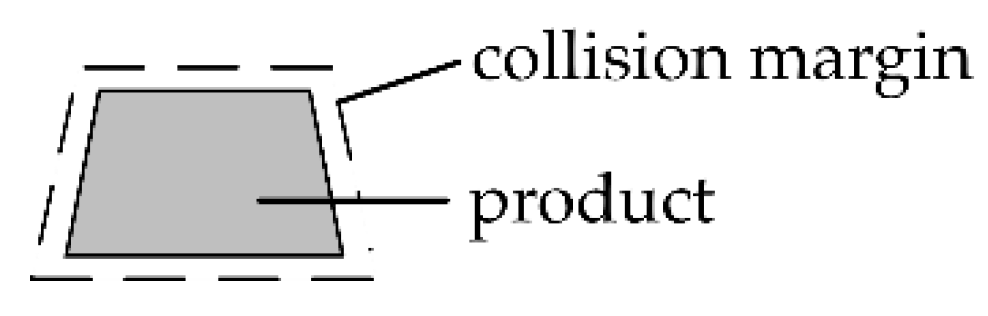
2.4. Disturbance Simulation

To investigate the machine model’s feasibility of simulating process disturbances in sufficient accordance with reality, possible disturbances of the example machine are recorded on-site under production conditions at a confectionary packaging company and are compiled to a disturbance list. Subsequently, all disturbances that cannot be simulated using VC software are not considered in detail within the simulation study. Three independent criteria regarding process and software are therefore taken into account:

• Can the process and disturbance-relevant behavior of the object be represented as in the model of rigid bodies?
• Can the process be modeled with 3D-CAD tools?
• Can the sensors be represented within the VC software?

The established criteria are based on the limitations of VC software to calculate the kinematic behavior of rigid bodies [20]. To take all affected parts of the process into account, the criteria differ depending on the considered machine level (the product and working tools, the process itself or the sensors). The first criterion is based on the restriction of the software to rigid bodies with regard to the products and working tools of the machine. The second one takes the restriction to rigid bodies and kinematic handling operations into account, regarding the process conducted on the machine. For instance, incorrectly wrapped confectionary cannot be simulated because of the product characteristics of the foil and the affected forming process. The third criterion addresses the limitation of VC software’s simulated sensors regarding detecting the kinematic or geometric properties of a product. An instance of a not-representable disturbance is the detection of chocolate pollution on the wrapped product, as an optical sensor cannot be modeled.

The disturbances meeting all three aforementioned criteria are hereafter assigned to one of four classes. As shown in

Table 1. Classification of disturbances representable within virtual commissioning (VC) software.

	Class 1	Class 2	Class 3	Class 4
Effect	Additional friction	Additional impact	Position change	Forcing sensor variable
Example	Products too high	Edge between conveyor belts	Broken products	Contaminated sensor
Simulated via	Changing product geometry	Changing machine geometry	Changing product geometry	Affecting switching characteristic

, these classes are set up with regard to the effects of the root causes on the process and supplemented by examples from the list. The interactions between several products and the machine are considered by classifying the disturbances in terms of their impacts on the discrete process; hence, this classification method is transferrable to other discrete processes. The first class includes disturbances wherein the relevant effect results in an additional location of friction within the process (for example too high products with contact to the upper guide rail). Disturbances within the second class are based on an additional location of an impact load. The root causes of disturbances of the third class provoke an immediate change of the product position within the process flow. Eventually, the causes of disturbances of class 4 affect the sensors directly by forcing their variables.

When choosing the disturbances to simulate, it is paramount to consider as many different root causes of disturbances as possible (e.g., machine settings, machine contamination, broken products, deformed products). The disturbances are simulated by modifying physical and geometrical parameters within the model (see Table 1). Therefore, the coefficient of restitution or friction is changed, the product or machine dimensions are adapted or a sensor signal within the machine model is set to a certain value. However, the simulative implementation of the cause of disturbance does not influence the class allocation. Changing the product geometry can be a modification of the outer product dimensions, as in the first class, or a division of the product into two parts, as in the fourth class. This changes in the model lead to a temporal switching behavior of the sensors, which is recorded. Interactions between different root causes of disturbances are not taken into consideration within this first step of examination. The simulation’s SR is set to 5 ms. To generate comparative data, an undisturbed process simulation is recorded as well. The results of the simulated process are evaluated visually during the simulation and analytically by comparing the recorded data of the switching behavior of the sensors over time.

3. Results and Discussion

3.1. Results of the Model Building Process

At first, the model was built within the VC software. To generate an error-free material flow through the machine sub-system, constructive adjustments were made in the relevant CAD-data, because the physics engine applies a collision margin of 1 mm to the simulated objects, as shown in Figure 6 [25]. Using the unadjusted CAD-files would lead to a geometrical error, exemplarily in the case of the product height. As the product height is below 10 mm, an additional margin of 1 mm on each side, added by the engine, leads to a geometrical deviation of more than 20% within the simulation. After building the model and conducting the simulation without disturbances, restrictions regarding the accuracy of the simulated material flow and simulation speed are determined. In the area of the gear (see Figure 3), a geometrically complex sorting process takes place. This process is not simulated correctly. This effect correlates with the statement in Hofman that objects smaller than 100 mm can cause instabilities within the calculations of the physics engine [31]. Therefore, that part of the gear is excluded from further analysis. Furthermore, time expansion already occurs when only this part of the machine is simulated with around 100 moving products, which limits the extension of the model to other machine parts subsequently.

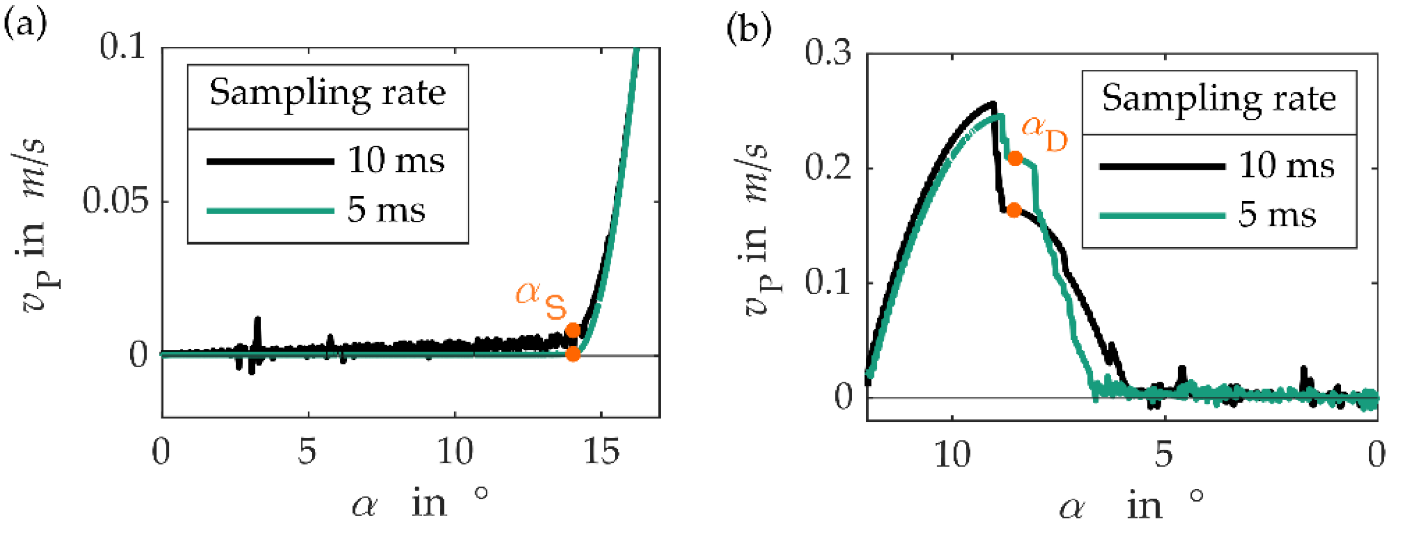
3.2. Results of the Verification

To conduct the experiment for static friction, the corresponding coefficient was set to default in the VC software,${\mu }_{\mathrm{S}}=0.25,$ which leads to an angle of ${\alpha }_{\mathrm{S}}=14.04°$ (Equation(1)). The results depictured in Figure 7a) imply that the coefficient is very sensitive to the SR. At a SR of 10 ms, the product slightly starts sliding prior to the analytically calculated angle ${\alpha }_{\mathrm{S}}$ and the velocity of the product vibrates during simulation. At a SR of 5 ms the accuracy increases, the product starts sliding at the angle ${\alpha }_{\mathrm{S}}$ and vibration disappears.

The coefficient of dynamic friction is generally lower than the static one. Due to the similarity of the experiment with Troll et al., the coefficient of dynamic friction is set to ${\mu }_{\mathrm{D}}=0.15$ too [30]. The verification of the coefficient of dynamic friction shows a sequence of velocity, as exemplarily depictured in Figure 7. For both SRs, a step in velocity before reaching the angle ${\alpha }_{\mathrm{D}}$ is visible. Furthermore, the velocity starts vibrating when converging to zero. According to Equation (2), the mean coefficient of friction ${\mu }_{\mathrm{D}}$ varies from 0.1521 ± 0.0009 (10 ms SR) to 0.1517 ± 0.0016 (5 ms SR) with relative errors $∆{\mu }_{\mathrm{D}}$ of 1.43% (10 ms SR) or 1.15% (5 ms SR) respectively, those being only marginally smaller with lower SR. Contrarily, the variance of the measurement data recorded at a SR of 5 ms is almost twice the variance at 10 ms SR.

To verify the coefficient of restitution, it is set to $k=0.4$ and the velocity of the component pushing the product is increased from $v_{\mathrm{coll}}=0.2$ m/s to $v_{\mathrm{coll}}=0.5$ m/s following [30]. The verification of the coefficient of restitution shows an overall decreasing relative error and a decreasing variance with increasing simulation’s SR (Figure 8), except at the product velocity of$v_{\mathrm{coll}}=0.45$ m/s. Depending on the scenario, both values fluctuate heavily. The maximum errors of the measurement data are 6.47% (SR of 10 ms) and 5.34% respectively (SR of ms).

The model verification reveals anomalies regarding the model calculation. Both experiments to verify the coefficients of friction show vibrations in velocity when converging to zero. In Hummel et al. the same behavior is described when using the engine BulletPhysics, which is explained with the impulse-based calculation algorithm applied within this engine [23]. This algorithm tends to get unstable when calculating stationary contacts [24]. Furthermore, an unwanted step in velocity within the verification of dynamic friction and a situational fluctuation of the model error within the verification of the coefficient of restitution are determined. The data recorded from all substitute tests are published alongside the manuscript as supplementary materials.

Despite those anomalies and by comparing the experimental values to the analytically ones, the program shows a generally sufficient physical behavior for the intended purpose. As to be expected, the calculated parameters for static friction and impact converge to the analytically determined ones when reducing the simulation’s SR, contrarily to calculating dynamic friction. A final statement on the relevance of the anomalies and the relative error of the model needs to be supported by a validation with real machine data.

3.3. Results of the Disturbance Simulation

For the simulation of disturbances, 28 out of 99 items on the compiled disturbances list meet the criteria to be simulated. Those disturbances are classified according to Table 1, whereat five are assigned to class 1, two to class 2, 15 to class 3 and six to class 4. Seven out of this 28 disturbances are exemplarily simulated in the set up model. From the disturbances assigned to class 1, the scenarios of an overly-low, adjusted upper guide rail and of overly-high products are simulated. The event conducted from the second class is an edge between two conveyor belts. As the third class contains the most disturbances, three examples were chosen to be simulated. The root causes of disturbances considered are broken products, products with lateral product remains from the previous production process and a contaminated conveyor belt. Eventually, from class 4 a contaminated sensor is represented in the model.

All of those seven disturbances have a visual impact during simulation and an impact on the recorded switching characteristic of the sensors. By comparing the simulated disturbance scenarios to the real one, different visual effects on the process can be identified. These visual effects are, for example, gaps within a group of products for classes 1 and 3, and a misalignment of products for class 2 and class 3, which, in case of class 3, partly causes products being sorted out. Disturbances of class 4 have no immediate impact on the process, but the machine runs out of products because the request for new products is stopped by the PLC. A similar visual effect can be detected simulating class 3 disturbances over a longer period of time, caused by sorted out products. Overall, the visual effects highly depend on the location of the root causes of disturbances and the functions of the affected sensors, which is why visual effects cannot be narrowed down to a specific class exclusively.

Each visual effect interrelates to a similar deviation in the switching characteristic of certain sensors, regardless of the disturbance root cause. Here, all sensors within the considered machine sub-system are photoelectric sensors. Switching characteristics are exemplary illustrated in Figure 9, compared to the data of an undisturbed production. As all sensor signals are binary data, signals 2 and 3 are multiplied by the factors 1.2 and 1.4 for better readability. Figure 9a shows the recorded time courses of the first three sensors while simulating products too highly, a disturbance of class 1. The disturbance results in additional short periods of the sensor not detecting products, due to additional friction between the product and the upper guide rail. The switching characteristics of sensor 2 and sensor 3 also show occasional short times not detecting products. The simulation of an upper guide rail too low adjusted shows a similar switching characteristic. Therefore, this effect is consistently observable with different disturbances of class 1. Figure 9b shows the impact of misaligned products on the switching characteristic when exemplarily simulating an edge between conveyor belts, a disturbance of class 2. This disturbance causes a variation in the actuation time period of the involved sensor. Two disturbances of class 3, the lateral product remaining and the contaminated conveyor belt, show similar influences on the switching characteristics of certain sensors. Figure 9c shows the switching characteristics resulting from simulating a contaminated sensor, a disturbance of class 4, provoking the machine to run empty. All sensors sequentially stop detecting products, according to their positions along the feeding unit, whereas the contaminated sensor shows a permanent actuation. Simulating the machine running empty by modelling a disturbance of class 3 results in similar switching characteristics, even though in this case all sensors stop detecting products and changes in the switching characteristics occur later, as there are still products arriving.

Altogether, it was possible to determine a reasonable outcome of the simulation model for all four classes of disturbances. Thus, VC software is generally able to generate test data for machine learning algorithms. When compared to the normal operational behavior of the machine, all simulated disturbances show logical deviations visually on the process and in the switching characteristics of the sensors. The amount of the deviation and the position of the affected sensor are strongly dependent on the considered disturbance.

4. Conclusions

This paper investigated the applicability of VC software to creating test data for machine learning algorithms. Therefore, a feeding system of an intermitting wrapping machine for confectionary was modeled within this software. Subsequently, replacement tests were carried out within the model verification to examine the model error. In the following model analysis, selected disturbances of the real machine were simulated and evaluated with regard to their effect on the process and the switching behavior of the sensors. To determine whether VC software has the ability to generate suitable test data for machine learning algorithms or not, this paper aimed to answer two main questions:

• To what accuracy can VC software simulate process disturbances?
• Is the achieved accuracy sufficient at depicting the effect of real operational machine behavior?

With regard to the first question, the first restrictions regarding the feasibility of VC software were determined when building the simulation model. Due to the size of this model, a time expansion occurred during simulation. Furthermore, restrictions regarding the calculation accuracy of geometrical complex and small parts were determined, which limits the transferability of the results to machines with a few, simple processing operations. Within the verification of the model, the overall, sufficient physical behavior and therewith the feasibility of the software for the intended purpose were determined anyway, with a maximum model error of 6.47%. Nevertheless, anomalies regarding the calculation of the physical parameters were identified.

Concerning the second question, the model analysis showed that only a limited number of process disturbances occurring on the machine can be simulated within the VC software. This restricts the proposed use of VC software to processes fulfilling the criteria set up in this paper. The disturbances that could be modeled with VC software were assigned to four classes. Changes in the sensor’s switching characteristics were determined in all four classes of disturbances and therefore an effect on the operational behavior was identified by simulating disturbances.

Eventually it was shown that VC software is generally usable for generating test data for machine learning algorithms focusing on simple discrete processes. The successful application of the software in this area can help to overcome the previous problems with the recording of process data. Therefore, the software enables investigations that focus specifically on individual disturbances and the normative operating behavior of the machine. By applying this method to a new machine it can finally help setting up an operator assistance system at the stage of initial commissioning.

Nevertheless, the correctness of the recorded data might be influenced by the error of the software’s calculation of parameters, as the root causes of the disturbances, on one hand, were implemented by varying these parameters, and on the other hand, cause effects related to these parameters. The influences of the model error on the wrapping process and the recorded data have not yet been investigated. An aspect of future research is therefore investigating the sensitivity of each parameter on the process and on switching characteristics separately. This will help determining the influence of each parameter’s error on the model and the generated data. Another step for investigating the suitability of the generated data to train an operator assistance system is the validation of the model. The model’s parameters need to be aligned to the parameters of the real system. Furthermore, the generated sensor data needs to be compared to the real system as well. Based on these results, interactions between root causes of disturbances, as they occur within the real process, could be simulated.

References

1. Schult, A.; Beck, E.; Majschak, J.-P. Steigerung der Effizienz von Verarbeitungs- und Verpackungsanlagen durch Wirkungsgradanalysen. Pharma + Food 2015, 18, 66–68. [Google Scholar]
2. Wandke, H. Assistance in human–machine interaction: A conceptual framework and a proposal for a taxonomy. Theor. Issues Ergon. Sci. 2005, 6, 129–155. [Google Scholar] [CrossRef]
3. Allais, I.; Edoura-Gaena, R.-B.; Gros, J.-B.; Trystram, G. How human expertise at industrial scale and experiments can be combined to improve food process knowledge and control. Food Res. Int. 2007, 40, 585–602. [Google Scholar] [CrossRef]
4. Perrot, N.; Agioux, L.; Ioannou, I.; Mauris, G.; Corrieu, G.; Trystram, G. Decision support system design using the operator skill to control cheese ripening––Application of the fuzzy symbolic approach. J. Food Eng. 2004, 64, 321–333. [Google Scholar] [CrossRef]
5. Edoura-Gaena, R.B.; Allais, I.; Gros, J.B.; Trystram, G. A decision support system to control the aeration of sponge finger batters. Food Control 2006, 17, 585–596. [Google Scholar] [CrossRef]
6. Kansou, K.; Chiron, H.; Della Valle, G.; Ndiaye, A.; Roussel, P. Predicting the quality of wheat flour dough at mixing using an expert system. Food Res. Int. 2014, 64, 772–782. [Google Scholar] [CrossRef] [PubMed]
7. Klaeger, T.; Schult, A.; Majschak, J.-P. Lernfähige Bedienerassistenz für Verarbeitungsmaschinen. Ind. 4.0 Manag. 2017, 33, 25–28. [Google Scholar]
8. Kong, L.; Peng, X.; Chen, Y.; Wang, P.; Xu, M. Multi-sensor measurement and data fusion technology for manufacturing process monitoring: A literature review. Int. J. Extrem. Manuf. 2020, 2, 1–27. [Google Scholar] [CrossRef]
9. Domingos, P. A few useful things to know about machine learning. Commun. ACM 2012, 55, 78–87. [Google Scholar] [CrossRef] [Green Version]
10. Müller, R.; Oehm, L. Process industries versus discrete processing: How system characteristics affect operator tasks. Cogn. Technol. Work 2018, 21, 1–20. [Google Scholar] [CrossRef]
11. Klaeger, T.; Schult, A.; Oehm, L. Using anomaly detection to support classification of fast running packaging processes. In Proceedings of the 2019 IEEE 17th International Conference on Industrial Informatics (INDIN’19), Helsinki-Espoo, Finland, 23–25 July 2019; Volume 1, pp. 343–348. [Google Scholar]
12. Lu, J.; Liu, A.; Dong, F.; Gu, F.; Gama, J.; Zhang, G. Learning under Concept Drift: A Review. IEEE Trans. Knowl. Data Eng. 2019, 31, 2346–2363. [Google Scholar] [CrossRef] [Green Version]
13. Reinhart, G.; Wünsch, G. Economic application of virtual commissioning to mechatronic production systems. Prod. Eng. Res. Dev. 2007, 1, 371–379. [Google Scholar] [CrossRef]
14. Lechler, T.; Fischer, E.; Metzner, M.; Mayr, A.; Franke, J. Virtual Commissioning—Scientific review and exploratory use cases in advanced production systems. Procedia CIRP 2019, 81, 1125–1130. [Google Scholar] [CrossRef]
15. Metzner, M.; Krieg, L.; Merhof, J.; Ködel, T.; Franke, J. Intuitive Interaction with Virtual Commissioning of Production Systems for Design Validation. Procedia CIRP 2019, 84, 892–895. [Google Scholar] [CrossRef]
16. Scheifele, C.; Verl, A.; Riedel, O. Real-time co-simulation for the virtual commissioning of production systems. Procedia CIRP 2019, 79, 397–402. [Google Scholar] [CrossRef]
17. Ayani, M.; Ganebäck, M.; Ng, A.H.C. Digital Twin: Applying emulation for machine reconditioning. Procedia CIRP 2018, 72, 243–248. [Google Scholar] [CrossRef]
18. Wünsch, G. Methoden für die Virtuelle Inbetriebnahme Automatisierter Produktionssysteme. Ph.D. Thesis, Technische Universität München, München, Germany, 2008. [Google Scholar]
19. Verein Deutscher Ingenieure. VDI/VDE 3693—Virtual Commissioning—Model Types and Glossary; Verein Deutscher Ingenieure: Düsseldorf, Germany, 2016. [Google Scholar]
20. Stich, P.; Krotil, S.; Reinhart, G. Interaktive simulationsgestützte Programmierung bei der Entwicklung mechatronischer Verpackungsanlagen. In Proceedings of the VVD 2015 Verarbeitungsmaschinen und Verpackungstechnik—8. Wissenschaftliche Fachtagung, Dresden, Germany, 12–13 March 2015; Majschak, J.-P., Ed.; Technische Universität Dresden: Radebeul, Germany, 2015. [Google Scholar]
21. Spitzweg, M. Methode und Konzept für den Einsatz eines Physikbasierten Modells in der Entwicklung von Produktionsanlagen. Ph.D. Thesis, Technische Universität München, München, Germany, 2009. [Google Scholar]
22. Boeing, A.; Bräunl, T. Evaluation of real-time physics simulation systems. In Proceedings of the 5th International Conference on Computer Graphics and Interactive Techniques in Australia and Southeast Asia—GRAPHITE ’07, New York, NY, USA, December 2007; ACM Press: Perth, Australia, 2007; pp. 281–288. [Google Scholar]
23. Hummel, J.; Wolff, R.; Stein, T.; Gerndt, A.; Kuhlen, T. An Evaluation of Open Source Physics Engines for Use in Virtual Reality Assembly Simulations. In Advances in Visual Computing; Bebis, G., Boyle, R., Parvin, B., Koracin, D., Fowlkes, C., Wang, S., Choi, M.-H., Mantler, S., Schulze, J., Acevedo, D., et al., Eds.; Springer: Berlin/Heidelberg, Germany, 2012; Volume 7432, pp. 346–357. [Google Scholar]
24. Lacour, F.-F. Modellbildung für die Physikbasierte Virtuelle Inbetriebnahme Materialflussintensiver Produktionsanlagen. Ph.D. Thesis, Technische Universität München, München, Germany, 2011. [Google Scholar]
25. Coumans, E. Bullet 2.83 Physics SDK Manual 2015. Available online: https://github.com/bulletphysics/bullet3/blob/master/docs/Bullet_User_Manual.pdf (accessed on 23 January 2019).
26. Drescher, B.; Stich, P.; Kiefer, J.; Strahilov, A.; Bär, T.; Reinhart, G. Physikbasierte Simulation im Anlagenentstehungsprozess—Einsatzpotentiale bei der Entwicklung automatisierter Montageanlagen im Automobilbau. In Proceedings of the Simulation in Produktion und Logistik 2013, Paderborn, Germany, 9–11 October 2013; Dangelmaier, W., Laroque, C., Klaas, A., Eds.; Heinz Nixdorf Institut (HNI): Paderborn, Germany, 2013; Volume 316, pp. 271–281. [Google Scholar]
27. Stich, P. Interaktiver Simulationsgestützter Entwurf mechatronischer Verarbeitungssysteme. Ph.D. Thesis, Technische Universität München, München, Germany, 2017. [Google Scholar]
28. Verein Deutscher Ingenieure. VDI 4465—Modellierung und Simulation: Modellbildungsprozess; Verein Deutscher Ingenieure: Düsseldorf, Germany, 2016. [Google Scholar]
29. Döring, M.; Majschak, J.-P. Berechnung von Bewegungsvorgaben unter Beachtung der Prozessdynamik am Beispiel des schnelllaufenden Transports von kleinstückigen Stückgütern. In Proceedings of the 10. Kolloquium Getriebetechnik—Berichte der Illmenauer Mechanismentechnik, Ilmenau, Germany, 11–13 September 2013; Universitätsverlag Illmenau: Ilmenau, Germany, 2013; Volume 2, pp. 187–200. [Google Scholar]
30. Troll, C.; Schebitz, B.; Majschak, J.-P.; Döring, M.; Holowenko, O.; Ihlenfeldt, S. Commissioning new applications on processing machines: Part I—Process modelling. Adv. Mech. Eng. 2018, 10, 1–11. [Google Scholar] [CrossRef]
31. Hofman, D. Simulationsgestützte Auslegung von Ordnungsschikanen in Vibrationswendelförderern. Ph.D. Thesis, Technische Universität München, München, Germany, 2014. [Google Scholar]
Figure 1. Triangulated surface of a cylinder based on [24].
Machines 08 00019 g001
Figure 2. Structure of the virtual commissioning test configuration based on [19].
Machines 08 00019 g002
Figure 3. Schematic structure of the investigated machine.
Machines 08 00019 g003
Figure 4. Inclined plane to verify the coefficient of friction.
Machines 08 00019 g004
Figure 5. Model to verify the coefficient of restitution.
Machines 08 00019 g005
Figure 6. Collision margin applied by BulletPhysics.
Machines 08 00019 g006
Figure 7. (a) Results of the static friction scenario; (b) results of the dynamic friction scenario.
Machines 08 00019 g007
Figure 8. (a) Impact at 10 ms sampling rate; (b) impact at 5 ms sampling rate.
Machines 08 00019 g008
Figure 9. (a) Switching characteristics simulating overly-high products (class 1); (b) switching characteristics simulating an edge between conveyor belts (class 2); (c) switching characteristics simulating a contaminated sensor (class 4).
Machines 08 00019 g009