1. Introduction
Energy supply has always influenced the geopolitical dynamics and coexistence of people. From the end of the 18th century, fossil fuels have been the main source of energy in the world, however, the energy crisis of the early 1970s, together with the gradual increase in awareness of the heavy environmental impact following the drastic global increase in the average terrestrial temperature, have progressively pushed technological research towards new sources of clean and renewable energy, first of all, wind and photovoltaics [
1]. The progress, although not enough from the point of view of environmental protection, is considerable. More countries are investing in large wind farms: this not only in the face of a greater awareness of the problems deriving from global warming and the drastic consequences they entail, but also to ensure greater political and economic independence from the countries that hold the oligopoly of fossil reserves by exploiting the resources already present, and unlimited, of the territory. In the field of wind power, considerable progress has been made in the optimization of medium-large size power systems. The costs to maximize their production, as well as production, are in fact contained with respect to the gains that can be obtained. Such rapid growth has obviously created the debate on the environmental impact due to these settlements, so that wind farms can be considered as a new source of environmental noise.
For clearly speculative reasons, due to the efficiency of the turbines, the wind farms are built in areas where the availability of wind is rich and continuous throughout the year [
2]. Italy, both for the geographical position and for the orography of the territory, has a good availability of sites suitable for the installation of wind farms, since, especially in the southern Mediterranean areas and islands, there are winds with a good intensity such as mistral, the tramontana, the sirocco and the libeccio [
3]. These areas are often located far from inhabited centers, but the continuous increase in investments has led to their enlargement so that the wind towers were built near the inhabited centers. The proximity to the urban settlements highlighted the problems deriving from the acoustic emissions generated by the wind towers during their operation. The wind towers generate a noise that is perceived as an annoyance by the population living near the wind farms. Studies on noise disturbance generated by the wind towers have been performed in different parts of the world that confirm the existence of this problem [
4,
5,
6]. Even if the generated sound levels are modest in the order of 30–50 dBA, this type of noise, for the sound component, is perceived as annoying, noise generation is one of the limits to the diffusion of wind farms [
7,
8].
Today there are various types of wind towers on the market, which differ in size and structure and are designed to support wind turbines of different sizes and power. A wind tower is not only a support structure but also allows the turbine to rise well above ground level, benefiting from the strongest winds blowing at higher elevations [
9]. The most widespread wind towers are over 100 m tall and have a blade radius of over 50 m. Although the speed of rotation of the blade is very low, about 15–20 rpm, the most distant point of the blade, compared to the axis of rotation, has a speed of about 300 km/h. The main noise components generated by wind turbines are the aerodynamic noise produced by rotating blades and the mechanical noise produced by the electromechanical parts (generator, revolutions, cooling systems, and other components). The mechanical component has a lower sound level than the aerodynamic one, and a few tens of meters away is no longer perceptible [
10]. The aerodynamic component, on the other hand, propagates and is also distinguishable from several hundred meters: In general, when sound propagates without obstruction from a point source, the sound pressure level decreases. Assuming a spherical propagation, the sound pressure level is reduced by 6 dB by doubling the distance. This simple spherical propagation model needs to be modified in the presence of reflecting surfaces and other disruptive effects including source characteristics, ground effects, blocking of sound from obstacles and uneven terrain, and meteorological effects [
11].
Recent Researches on the Subject
There are several approaches to the problem of noise propagation produced by wind turbines. As already mentioned, a simple identification as a point source and the related propagation in an open field is not able to explain the phenomenon. This is due to the orography of the territory which has a strong dynamic effect on the movement of the air given by phenomena such as wind acceleration and deceleration, ascending and descending currents, turbulent vortices, and forced channeling. To these are added the reflective and shielding effects produced by the ground and vegetation. The numerous studies conducted on the subject highlight the importance of the problem. Guarnaccia et al. [
12] studied the acoustical noise of a turbine considering the mathematical properties of the propagation function. They propose to treat the propagation function near the turbine as a function like Lorentziana. Forssén et al. [
13] evaluated the variation of emission sound levels under the influence of meteorological variation. The results obtained show that meteorological factors influence the noise generated by the wind turbine rather than the sound propagation. Son et al. [
14] predicted noise generated from wind turbine using integrated numerical methods. Furthermore, using further numerical method the authors adjusted aerodynamic loadings and aerodynamically generated sound. Receiver regions have been affected by broadband noise even in far field. Terrain effects are confirmed as important factors. In this study, the effects of the temperature gradient and wind speed variation were not considered.
Barlas et al. [
15] developed a numerical technique that models the sound propagation from the source to the receiver. Large eddy simulation with an actuator line technique is applied for the flow modeling and the corresponding flow fields are employed to simulate sound generation and propagation. Sound pressure level data measured at the turbine are elaborated for varying wind speeds, surface roughness, and ground impedances within a 2 km radius from it. Barlas et al. [
16] treated the wind turbine noise propagation in flat terrain for use in wind farm layout optimization frameworks. Large-eddy simulations of a single wind turbine in flat terrain at different wind speeds, shear, and turbulence levels are developed. The wind turbine is modeled applying an actuator line approach, while the wind turbine noise propagation is calculated using a wind turbine simulation tool. The authors’ purpose was to develop a noise propagation database that can be employ as a lookup table in wind farm layout optimization frameworks to reduce the noise impact in the project of new wind farms.
In recent times machine learning-based algorithms have been applied in the field of wind turbines. Several works concerned the prediction of the wind turbine power according to the available wind power series [
17,
18,
19,
20,
21,
22,
23,
24]. Other works studied the fault diagnosis of wind turbines, referred to the blades and to the gearbox [
25,
26,
27,
28,
29,
30,
31]. Other authors have instead developed models for predicting wind speed to be used in choosing the location to install wind turbines, or as a tool to support the management of a wind farm [
32,
33,
34,
35,
36,
37]. Machine learning is based on the availability of large amounts of data and computing power. Rather than making hypotheses a priori, machine learning allows the system to learn from data. Rather than following preprogrammed algorithms, it uses data to build and continuously refine a model to make predictions. It helps to understand the propagation of noise produced by wind turbines by detecting and modeling the attributes that define its profile. Learn from the data and modify the processes accordingly. In this context the contribution of the researcher becomes crucial to guide the construction of models based on automatic analysis. Through Visual Data Analytics it is possible to extract knowledge from visualization, from automatic analysis, as well as from previous interactions between visualizations, models, and researchers [
38].
In the present work, the results of the measurements carried out within a dwelling located near a wind farm in southern Italy were analyzed. In addition, data on the power generated by wind turbines and wind speed near the nacelle were analyzed. These data were used for the development of a model able to predict the levels of environmental noise near the receiver.
The assessment of environmental noise at the receiver near the wind farms is a difficult task for the experts in the field. This is since the environmental noise is strongly correlated both to the wind speed and to the noise emitted by the turbines. However, the relationship between environmental noise and wind speed is not easily predictable, especially in hilly areas, where the changes in wind intensity and direction are remarkable. In these cases, a tool for predicting sound pressure levels at the receiver based on wind speed and the active power generated by the turbines can be extremely useful. Through the results of the model, it will be possible to establish which wind speed values the noise produced by wind turbines become dominant. Indeed, at low wind speeds the contribution to the environmental noise caused by the wind is negligible compared to the noise deriving from the operation of the turbines. In these environmental conditions the noise produced by wind turbines can be annoying to the receiver. Moreover, the predictive model can be a valid tool for the wind farm manager who can use it to get an overview of the noise produced by the plant in the different operating conditions. Finally, the prediction model does not require the shutdown of the plant, a very expensive procedure due to the consequent production loss.
2. Methodology
The study was conducted in a rural area of southern Italy. It is a hilly area located in a depression between two mountains, and between two streams. The territory has typical landscape features of the southern Italian Apennines: extensive woods of oaks and oaks, and residues of the forest. The soils are of various kinds: clayey, anhydrite, silico-clastic, and carbonate. In this area, there is a wind farm with four wind turbines. The wind turbine under investigation is of the horizontal axis type with a nominal power of 2 MW [
39]. The towers are of a monopolar tubular type and hub height of 80 m, equipped with three blades with a diameter of 95 m, made of glass fibers. The maximum power is obtained at a speed range from 12.5 m/s to 25 m/s. Beyond this speed the blades stop for safety.
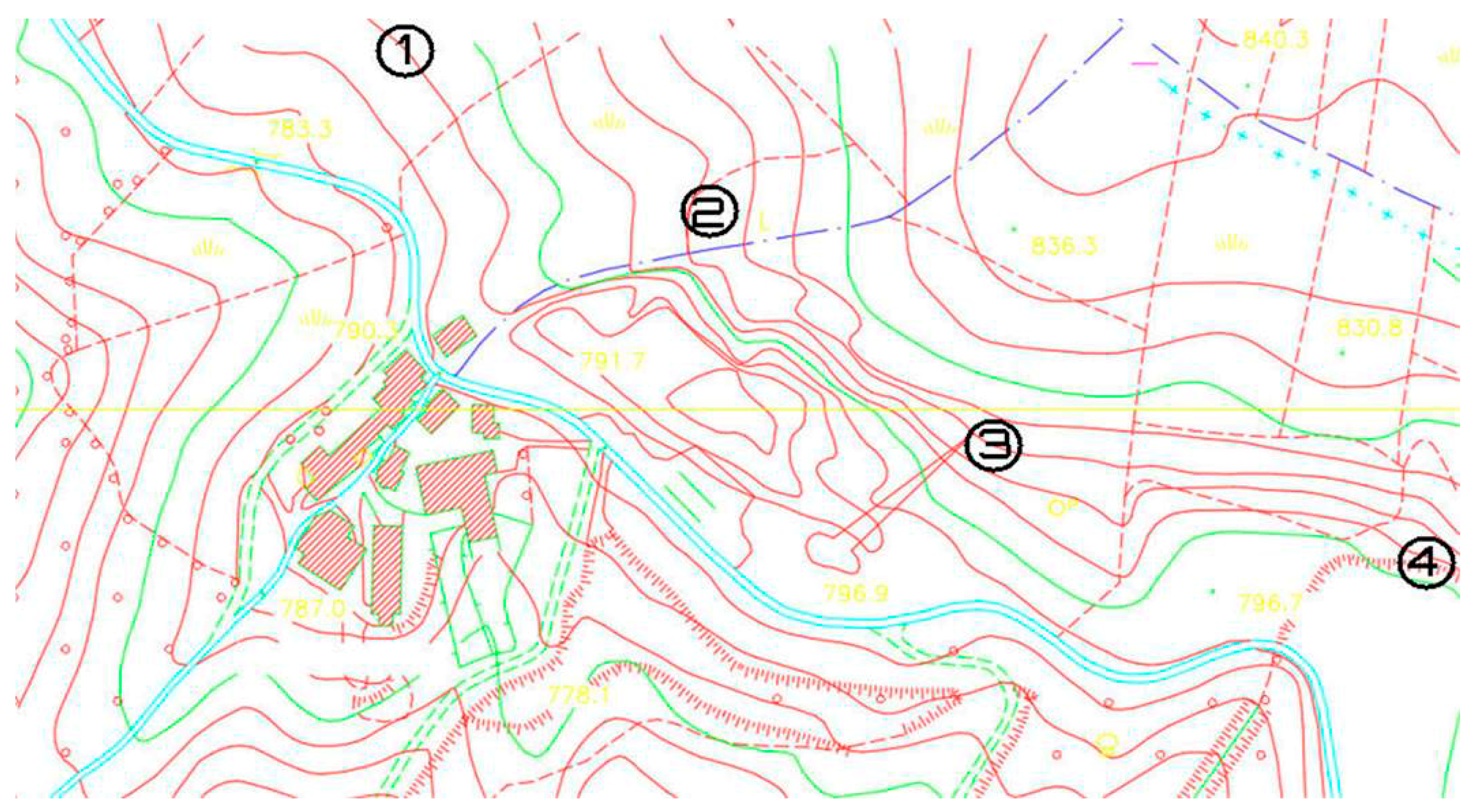
To predict wind turbine noise, the closest receiver to the installation of the wind turbines was identified. With respect to this receiver, the towers are positioned at the following distances: tower 1, 230 m, tower 2, 250 m, tower 3, 400 m, tower 4, 780 m. The distances between the wind turbines and receiver were estimated using global positioning system (GPS) data.
Figure 1 shows the locations of the towers respect the receiver.
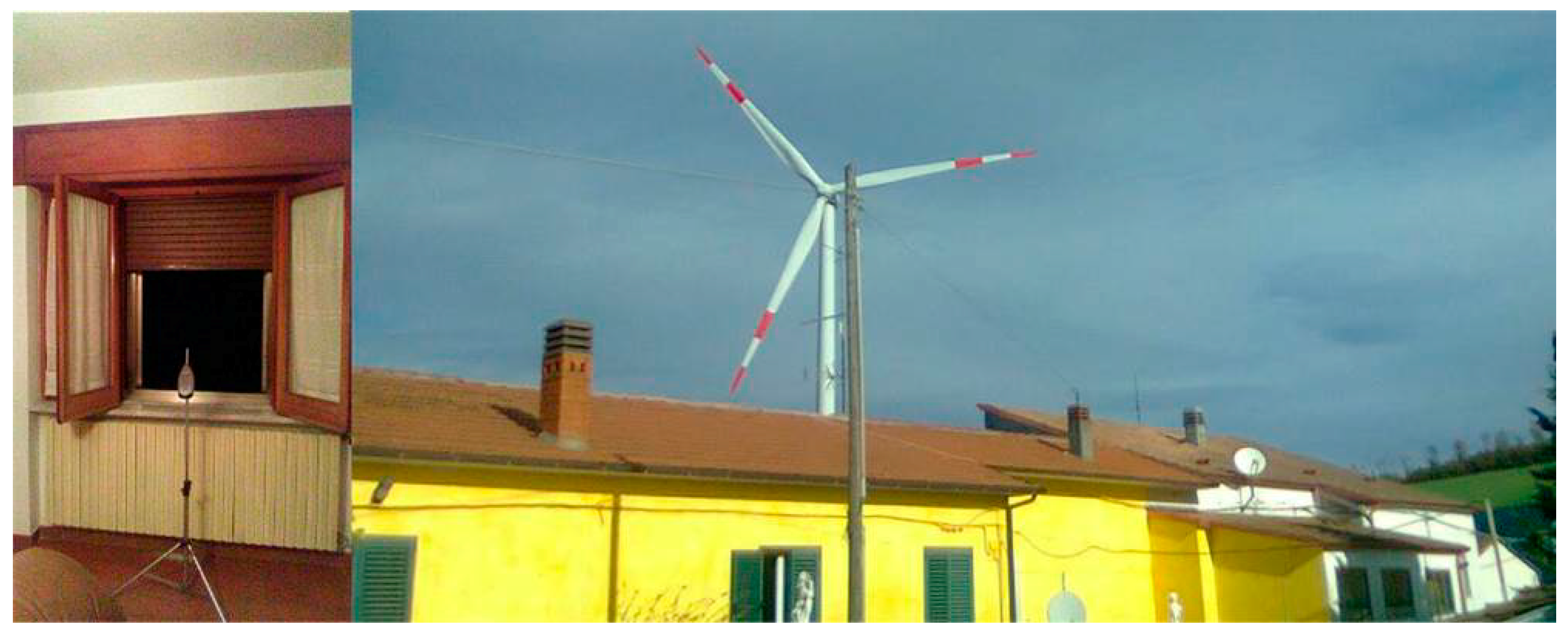
The acoustic measurements were performed inside a private house near the wind farm, with open windows (condition of maximum disturbance), using a sound level meters placed in a room. The sound level meter was installed on a tripod at a height of 1.60 m from the floor and 1.20 m from the window, 2.00 m wide and 1.20 m high. The normally furnished room (bedroom) was 5.0 m wide, 4.0 m long and 3.0 m high [
40]. For acoustic measurements the following instrumentation was used:
Figure 2 shows the equipment during the acoustic measurement process (on the left) and a view from the window of the house where it is clearly possible to identify one of the 4 turbines (on the right).
The instrument used to comply with the requirements of the IEC61400-11 standard [
41]. The sound level meter has been configured for the acquisition of the equivalent level of linear sound pressure, weighted “A”. The acoustic measurements were performed during the night with all wind turbines in operation.
During the measurements, the power generated by the turbine and the wind speed were recorded near the nacelle using a supervisory control and data acquisition (SCADA) system [
42,
43]. A SCADA system allows us to have remote control and supervision of the entire wind farm and individual wind turbines. These systems produce a lot of data at normally 10-min resolution, however, the type of signals recorded can differ largely depending on the turbine type. The SCADA system can be run on a computer in the control room of the wind farm or it can be run on any computer connected to the Internet that accesses the wind farm via TCP/IP protocol. This system provides useful real-time information on the operation of each individual turbine.
In addition to providing this useful information, a SCADA system allows you to start/stop the entire wind farm, turbine groups or individual wind turbines. Furthermore, the turbine control can be used to set production limits or to stop the operation of the turbines in case of anomalies or too strong wind. The turbines are equipped with the SCADA system based on IEC 61400-25.
The following variables were extracted:
WEC1Ac: Active power (kW) measured at Wind Turbine 1
WEC1WS: Wind speed (m/s) measured at nacelle of the Wind Turbine 1
WEC2Ac: Active power (kW) measured at Wind Turbine 2
WEC2WS: Wind speed (m/s) measured at nacelle of the Wind Turbine 2
WEC3Ac: Active power (kW) measured at Wind Turbine 3
WEC3WS: Wind speed (m/s) measured at nacelle of the Wind Turbine 3
WEC4Ac: Active power (kW) measured at Wind Turbine 4
WEC4WS: Wind speed (m/s) measured at nacelle of the Wind Turbine 4
These variables will be used as predictors in the prediction model.
Subsequently, the acoustic measures and the SCADA data were used to implement a model based on the Random Forest algorithm for the automatic prediction of the noise emitted from the wind turbines at the receiver [
44].
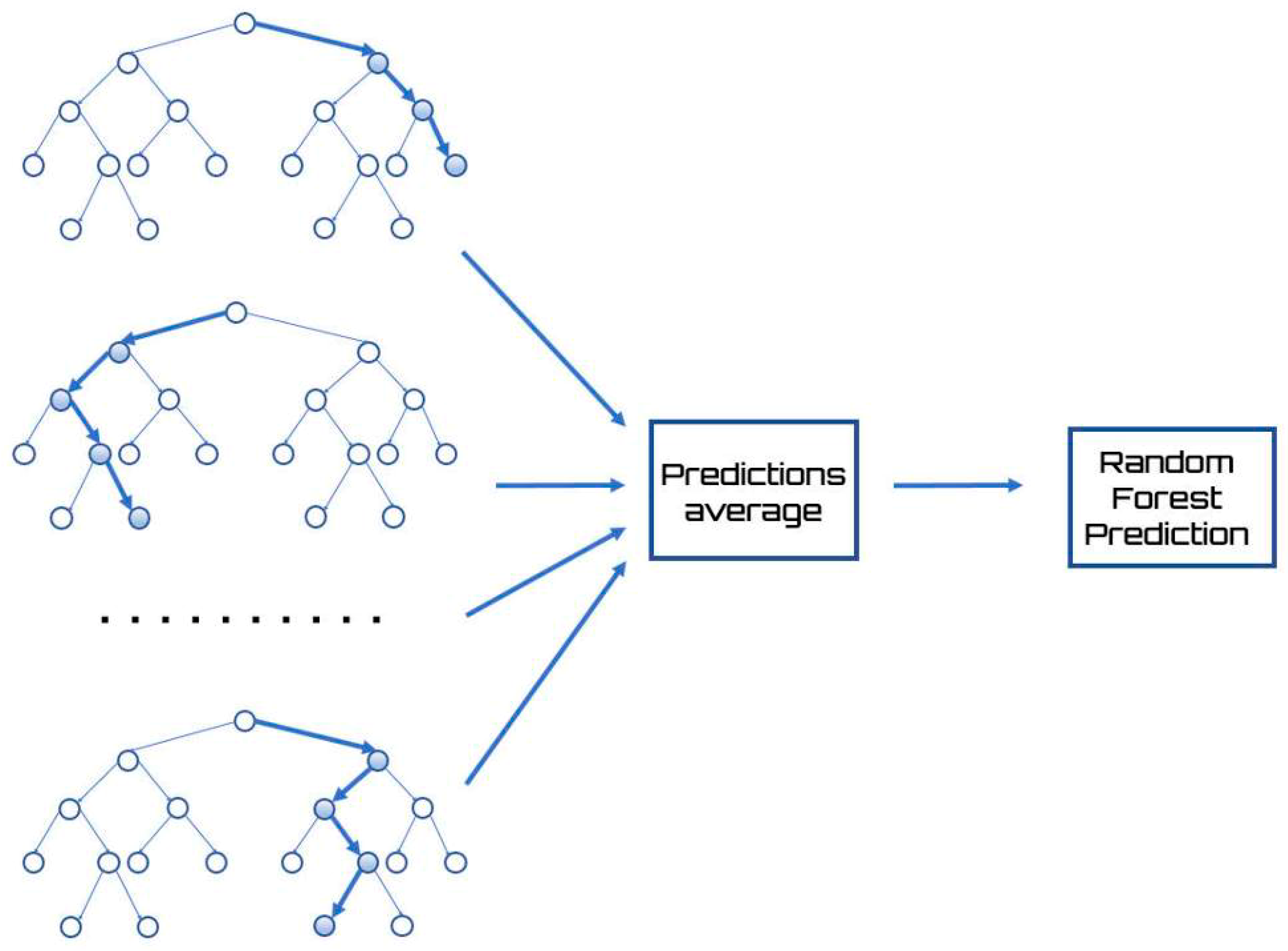
Random forests are a very powerful tool and can be used for both classification and regression. Regarding regression, a multitude of decision trees are constructed, and the output of each tree is obtained as output. As in the other cases of regression, even random forests train with supervised learning, providing a value based on input values and training with a multitude of examples.
A Random Forest is a special classifier formed by a set of simple classifiers (Decision Trees), represented as independent and identically distributed random vectors, where each of them votes for the most popular class in input [
45]. This type of structure has made noticeable improvements in the accuracy of learning by classification/regression and falls within the sphere of the ensemble learning [
46]. Each tree within a Random Forest is constructed and trained from a random subset of the data in the training set. Therefore, the trees do not use the complete set, and the best attribute is no longer selected for each node, but the best attribute is selected from a set of randomly selected attributes. Randomness is a factor that then becomes part of the construction of classifiers and aims to increase their diversity and thus reduce correlation.
The result returned by the Random Forest is none other than the average of the numerical result returned by the different trees in the case of a regression, or the class returned by the largest number of trees in case the Random Forest was used to perform classification.
Figure 3 shows a diagram of the Random Forest method.
A linear regression model is used for the prediction of continuous values. This model will help us to compare the results obtained with the model based on the Random Forest algorithm. Linear regression consists of learning an approximate function of available input-output pairs. The approximate function is in the form f (x) = y where y is a numerical value and continuous in R. The independent variable x is assumed to be exact while the dependent variable y is assumed to be affected by error [
47].
3. Results
3.1. Acoustic Measurements and SCADA Data Analysis
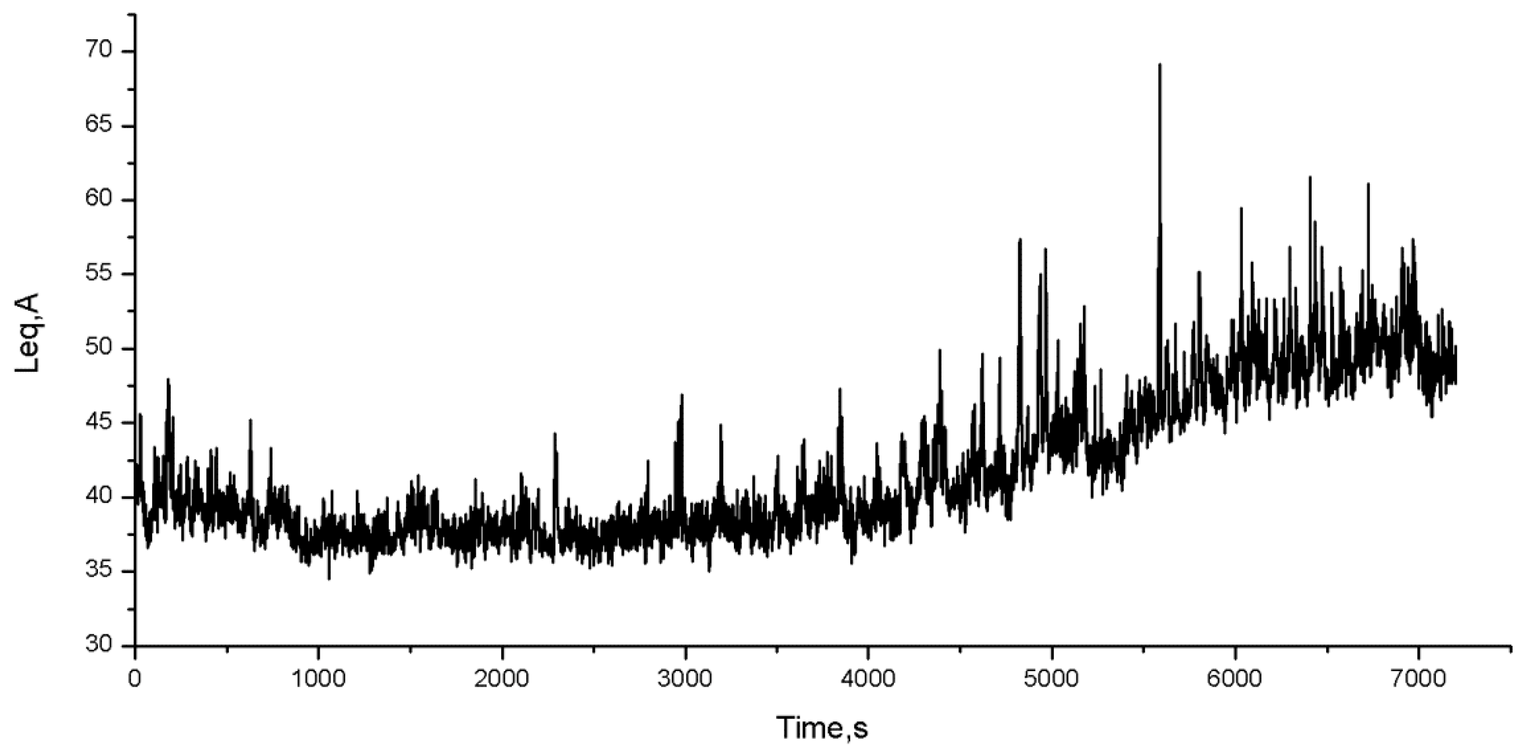
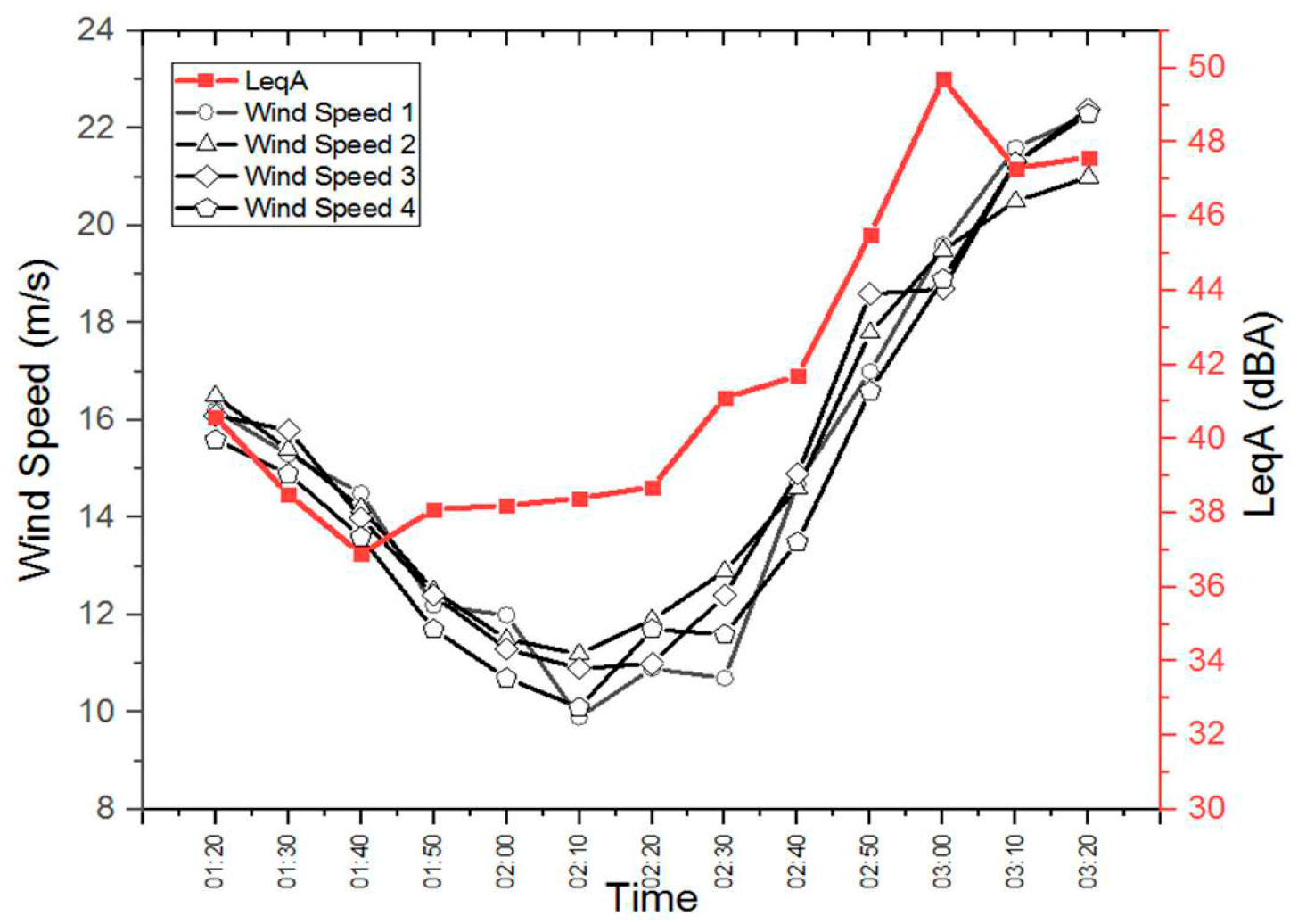
The acoustic measurements were made during the nighttime in the month of February, with wind speeds ranging from a minimum of 9.9 m/s to a maximum of 22.4 m/s. During the measurements, all turbines were switched on. Measurements started at 1:20 am and ended at 3:20 am with duration of 2 h.
Figure 4 shows the time history of the sound pressure level for the operating conditions performed in the measurement session.
Figure 4 shows the possibility to identify different environmental noise conditions. In fact, the background noise decreases in the first period and then undergoes a considerable increase in the second part of the monitoring period. To understand what happened during the measurement session we can analyze the data recorded by the supervisory control and data acquisition (SCADA) system. In
Table 1 are shown SCADA data for all wind turbines measured at 10 min intervals.
As already specified above, during the monitoring period, the wind speed has varied in the range 9.9–22.4 m/s. Variations in wind speed determine different values of electricity production, as can be read in
Table 1. From the reading of this Table it is also possible to find confirmation what has been said previously: The maximum power is obtained in a speed range from 12.5 m/s to 25 m/s. In fact, within this range while increasing at wind speed, production remains almost constant. For safety reasons when the speed exceeds 25 m/s the control system (SCADA) stops the blades.
Figure 5 shows the trends of active power and wind speed in the monitoring period for all 4 turbines.
From the analysis of
Figure 5, it is possible to notice that for all 4 turbines there is a decrease in active power in correspondence with a marked decrease in wind speed. When the wind speed drops below 12.0 m/s, there is a decrease in the active power which returns to an almost stationary value when this speed returns to values above 12 m/s. Turbine 3 at the final part of the observation records an abnormal reduction in power not in line with the value of the recorded wind speed and with the trend shown by the other turbines. This trend is due to a gradual shutdown of the turbine imposed by the control system (SCADA).
It should be noted that although the variation of the active power generated by the turbines undergoes a modest variation and for a short period, the variation in wind speed was significant. This fact assumes relevance since the wind is itself a significant source of noise [
48,
49,
50].
Table 2 shows the min and max values for active power and wind speed registered in the period under analysis.
As previously stated, the minimum value of the active power recorded for turbine 3 refers to a phase of progressive stopping of the turbine. Analyzing the extensive variability in wind speed arises the need to compare this trend with that obtained from noise measurements.
Table 3 shows the wind speed values measured near the 4 turbines and the sound pressure levels measured during the observation period.
Table 3 shows that the LeqA first decreases and then progressively increases until it reaches the maximum values recorded in the final part of the observation period. This trend reproduces the same trend observed for the variation of wind speed suggesting a connection between the two events. However, to observe in more detail how these values are distributed it is advisable to draw a graph as shown in
Figure 4.
Figure 6 shows what emerged from the reading of
Table 3 is confirmed. In particular we can note that in the extremes of the observation period the LeqA trend follows exactly that of the wind speeds: first, it undergoes a decrease and then progressively increases until it reaches maximum values recorded in the final part of the observation period. The central part of the graph instead tells us something different: In this area to a further decrease in wind speed that reaches its minimum values does not correspond a relative decrease in the LeqA that instead increases. This phenomenon can be explained by the fact that at low wind speeds the contribution to the environmental noise caused by the wind is negligible compared to the noise deriving from the operation of the turbines [
39]. In this period, moreover the graph shows an almost constant trend of the noise to confirm that it is the noise generated by the turbines. The phenomenon is reversed at high wind speeds where the contribution to the environmental noise deriving from the wind becomes predominant compared to that deriving from the turbines. The noise peak recorded at 3:00 am (LeqA = 49.7 dBA) is presumably due to anthropogenic activities that were added to the contribution deriving from the activity of the wind and from that deriving from the wind farm.
3.2. Data Processing
As we have anticipated, our goal is to use the data obtained from the SCADA system to implement a model based on the Random Forest algorithm for the automatic prediction of the noise emitted by wind turbines. To build a prediction model the measured data were resampled by setting as a 1 s integration time. A total of 7200 observations were collected and 8 variables were selected as predictors and 1 variable as a response. It is, therefore, a question of seeking a relationship between measurements of active power (kW), wind speed (m/s), and sound pressure level (dBA). Each variable contained in the input data (active power (kW) and wind speed (m/s)) has a different unit of measurement and range of values. In these cases, if a variable has significantly higher numerical values than the others it will be dominant in the knowledge extraction procedure. In this way all the content represented by the other variables will be lost with the result that the model developed will be limited.
If this happens, it is necessary to treat the data adequately and preventively with the aim of weighting the descriptors so as to represent the measured phenomenon in the best possible way. The procedure that allows us to solve this problem is called data normalization. This procedure makes the descriptors comparable by standardizing them on the basis of the same standard. In this way, two results are obtained essentially: the polarity is inverted, and the data are transformed into pure numbers eliminating the dimensions.
The normalization was carried out using the Min-max normalization method [
51]. In this way, the original data is transformed linearly by returning all the data in the interval (0.1). The Min-max normalization is based on the following formula:
It is important to specify that the Min-Max normalization preserves the relations between the values of the original data. However, having this limited interval has a disadvantage: we will get smaller standard deviations, which in some cases can induce a masking effect of the outliers.
The final objective of our model is not so much to find an exact prediction of the data in our possession (already labeled), but to determine a good prediction concerning new input data (not labeled). If we elaborate a model with few coefficients we will give rise to a very poor interpolation, instead if we interpolate too many of them we risk taking into consideration also the noise and therefore having poor results. Indeed, raising too many orders the degree of the polynomial with which we interpolate the data, we risk finding ourselves faced with an overfitting phenomenon, which has an error function equal to zero, but with very few results concerning the prediction of new data. Substantially decreasing the degrees of freedom of the aforementioned polynomial the function of error concerning the training data will always be closer to zero, but what concerning the test data at a certain point will tend to go up again. The degrees of freedom is related to the number of weights, that is to the number of hidden units on the network, so our goal is to find the optimal number of hidden units in order to have the best performances with test data.
To measure the performance of a network we must then divide the data into two independent sets, which are called training and test sets so that we can check how the error varies on both learning and new data introduced later. Only in this way can we find the best-hidden number m of units for the network, we must ensure that the network has enough flexibility, but does not give rise to overfitting. The network to function optimally must have a low error regarding the test data. In our case we have divided the data in our possession into two sets: training set equal to 70% of the data, and test set equal to the remaining 30% of the data. The subdivision of the observations in the two together was carried out randomly.
3.3. Linear Regression Analysis
First, to obtain predictions about the sound pressure level generated by turbine operation, a model based on multiple linear regression was used. This model will serve us later to make a comparison with the results obtained with the model based on the Random Forest algorithm that we expect to be more efficient.
To perform a regression analysis the Generalized Linear Models (GLM) was used [
52]. GLMs are extensions of traditional regression models that allow the average to depend on explanatory variables through a link function and the response variable to be any member of a set of distributions called exponential family (such as Binomial, Gaussian, Poisson, and others). The glm() function of the R software was used [
53]. The model is specified by giving a symbolic description of the linear predictor and a description of the error distribution. The response distribution as Gaussian and the link function from the expected value of the distribution to its parameter as identity were specified. We have included a family of additional arguments to describe the distribution of errors and the link function to be used in the model.
To measure the model performance the Root Mean Squared Error (RMSE) was calculated [
53]. The RMSE is the square root of the mean squared error, it is the standard deviation of the deviations between the values of the observed data and the values of the estimated data. The RMSE is a good measure of precision but can only be used to compare estimates referred to the same variable, as it depends on the same metric, not being a dimensionless index. The RMSE varies between zero and + ∞ and indicates a worsening of the performance as the value increases.
Another indicator of the model’s performance is the correlation coefficient. We used Pearson’s correlation algorithm between the actual and the predicted values [
53]. The values of the correlation index vary between -1 and +1, both extreme values represent perfect relations between the variables, while 0 represents the absence of relation. In
Table 4 are shown the RMSE value and the Person’s correlation coefficient for the multiple regression model.
Table 4 shows a Root Mean Squared Error equal to 0.003788142, this is a very low value indicating a good prediction of the response variable. Person’s correlation coefficient is very close to 1 (0.897) indicating also a good performance of the multiple regression model. Further information can be obtained by comparing this model with the one based on the Random Forest algorithm.
3.4. Random Forest Model
As we already said, a Random Forest model is a special classifier formed by a set of simple classifiers (Decision Trees), represented as independent and identically distributed random vectors, where each of them votes for the most popular class in the input. Breiman’s random forest algorithm was used [
45]. Breiman has shown that substantial gains in regression accuracy can be obtained by using sets of trees, where each tree is cultivated according to a random parameter. The final forecasts are obtained by aggregating all the trees to form a whole. Random Forest does not require the implementation of cross-validation techniques or verification on a separate set of variables to have an impartial evaluation of the error, as this is intrinsically guaranteed by the method. Each tree, in fact, is built using a different bootstrap sample of the original data, while the cases not selected for the tree construction are used to estimate the errors of the model. This model is easy to use since it provides for the insertion of only two parameters (the number of variables in the subset of random variables used in each node and the number of trees in the forest) and is not very sensitive to their values.
The Breiman algorithm allows us to measure the importance of the predictor variable and returns a measure of the internal structure of the data (proximity). The importance of the variable is difficult to determine, because it may be due to the possible interaction with the other variables. Breiman [
54] proposed four different measures that quantify the relevance of each variable. The first method evaluates the importance by looking at how much the forecast error increases when, in Out-of-bag (OOB) cases, the values of the considered variable are changed, while all the others remain unchanged. In the following two methods, at the end of the simulation, the margin of the nth statistical unit is considered. The margin is given by the proportion of the votes for its true class of membership (note) minus the maximum between the proportions of votes for each of the remaining classes. In the second method, the m-th variable is obtained as the average of the margins which are lowered for each case when the m-th variable is permuted as in the first method. In the third method, the count of how many margins have been lowered, less the number of margins that have risen, is represented. Finally, in the fourth method, for each subdivision, one of the variables is used to form the subdivision, an event that involves a reduction in the Gini index. The sum of all the decreases in the forest due to a certain variable, normalized by the number of trees, constitutes the measure.
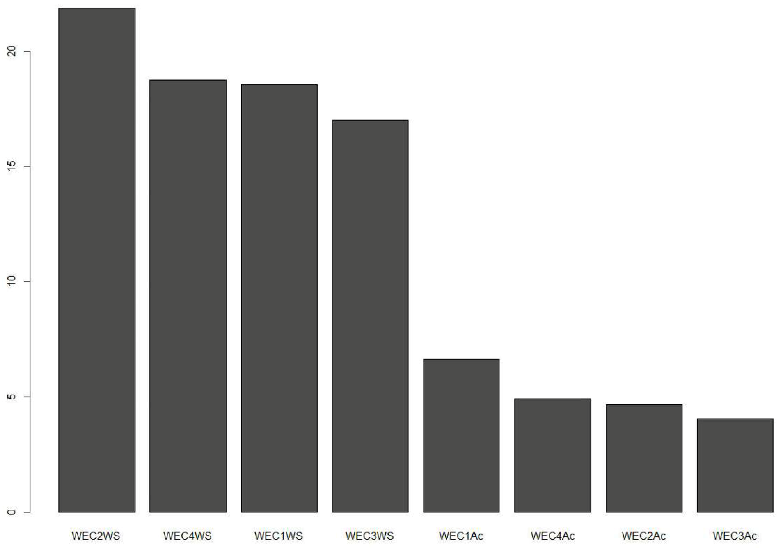
Figure 7 shows the importance of the variables of the Random Forest Model predictors.
Figure 7 shows that in the prediction of sound pressure levels, the data relating to wind speeds detected near the turbines are of greater importance. The turbine 2 seems to be the one that most influences the forecast, this is due to its proximity to the receiver. In fact, as shown in
Figure 1 the turbine 2 is located only 250 m from the house where the sound pressure levels were measured. Moreover, due to the conformation of the terrain, the turbine 2 provides the greatest contribution to the environmental noise detected at the receptor.
Figure 5 shows the wind speeds detected near the other turbines, whose importance is determined by the distance from the receptor but also depends on the conformation of the terrain. At the end of the graph, we find the data relating to the active power. These data are essential in the management of the period in which even though the wind speed is lowered, the LeqA remains almost constant. As previously mentioned, in this phase the contribution to the environmental noise provided by the operation of the wind turbines is predominant compared to that due to the wind.
Table 5 shows the RMSE value and the Person’s correlation coefficient for the Random Forest model.
Table 5 shows a Root Mean Squared Error equal to 0.003788142, this is a very low value indicating a good prediction of the response variable. Person’s correlation coefficient is very close to 1 (0.981) indicating also a good performance of the Random Forest model.
From the comparison between the two models (multiple regression and Random Forest), we can obtain useful information on performance. From the comparison of the data reported in
Table 4 and
Table 5, we can see that the model based on the Random Forest algorithm shows better results: Random Forest Person’s correlation coefficient equal to 0.981 compared to 0.897 obtained with Generalized Linear Model. Furthermore, the Random Forest model has a decidedly lower error with 0.0007370879 compared to 0.003788142, with an order of magnitude less.
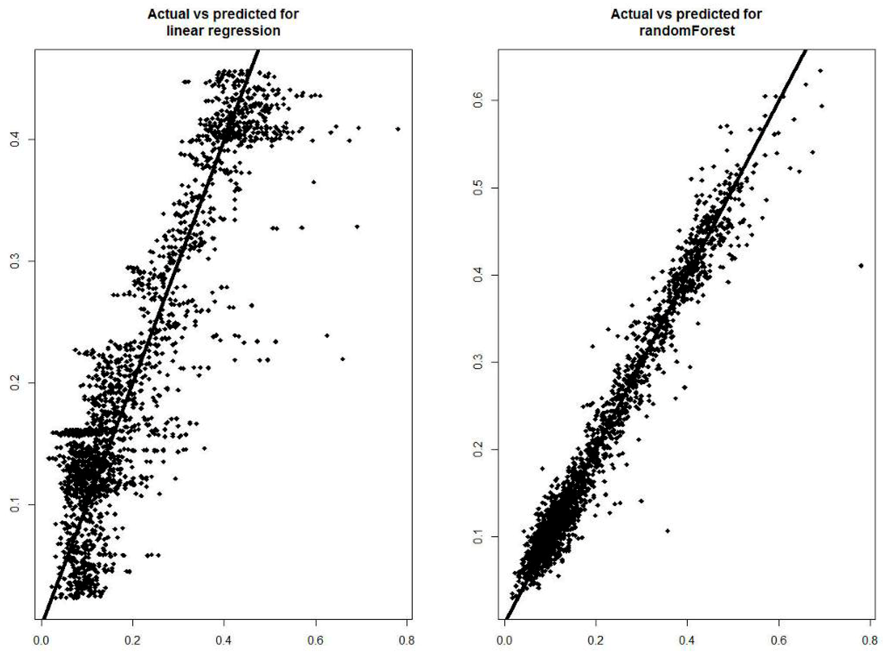
Figure 8 shows actual versus predicted values for both the tested models.
Figure 8 shows the difference between the two models: in the Random Forest, the data are grouped more around the line showing only a few isolated cases to indicate that the predicted data are like the actual ones. The model based on the multiple linear regression instead shows a greater number of isolated cases that deviate more from the line to indicate a greater margin of errors.
4. Discussion
From the analysis of the environmental noise measures (
Figure 4), we can notice that the background noise decreases in the first period and then undergoes a considerable increase in the second part of the monitoring period. The measured noise gradient cannot be only attributable to the noise produced by wind turbines but must be mainly due to the noise produced by the wind which in the second part of the monitoring period increases considerably in speed (from 9.9 to 22.4 m/s).
From the analysis of the SCADA data (
Figure 4) it should be noted that although the variation of the active power generated by the turbines undergoes a modest variation and for a short period, the variation in wind speed was significant. This confirms what has just been said: The measured noise gradient cannot be only attributable to the noise produced by wind turbines.
The final confirmation comes from the analysis of
Figure 5: In the central part of the noise monitoring to a decrease in wind speed that reaches its minimum values does not correspond to a relative decrease in the LeqA that instead increases. This phenomenon can be explained by the fact that at low wind speeds the contribution to the environmental noise caused by the wind is negligible compared to the noise deriving from the operation of the turbines. All this tells us that the available data must be integrated in order to build a model for predicting ambient noise levels at the receiver.
The forecast model based on the Random Forest algorithm showed the value of the Person’s correlation coefficient equal to 0.981, indicating good performance of this model. Analyzing
Figure 7 (Actual versus predicted values) it is possible to notice that all the values are placed on the line to indicate that the error committed in the forecast is negligible.
The results obtained are consistent with other available literature studies, which used models based on the Random Forest algorithm to make predictions. Wang et al. [
55] used the Random Forest algorithm, to perform the hourly forecasting of electricity needed for two school buildings in north-central Florida. The models trained with different parameter settings were compared to study the impact of parameter setting on the predictive performance of the model. They then compared the results obtained with the Random Forest with models based on the Regression Tree and Support Vector Regression. The comparison showed the superiority of Random Forest in the realization of energy predictions. Kusiak et al. [
56] used different data mining algorithms to develop prediction models for faults of 17 wind turbines. Random forest algorithm models provided the best accuracy among all tested algorithms. The solidity of the predictive model is validated for failures that have occurred on turbines with data never seen before. Lahouar et al. [
57] used Random Forest algorithm to obtain an accurate forecast of wind energy in the hour. They studied the effect of wind speed and direction on model performance and demonstrated how the Random Forest is not sensitive to irrelevant inputs. The results of this study show improvements in the accuracy of the forecasts and an important reduction of the errors compared to the prediction made with a model based on neural networks.
5. Conclusions
In recent years the algorithms based on machine learning have been used in various fields [
58,
59,
60,
61,
62,
63,
64,
65,
66]. In this study, the measurements of the noise emitted by a wind farm and the data recorded by the SCADA system were used to construct a prediction model. First, acoustic measurements and SCADA data have been analyzed to characterize the phenomenon [
67,
68,
69,
70]. An appropriate number of observations were then extracted, and these data were pre-processed. Subsequently, two models were built for the prediction of sound pressure levels at the receiver, based on the machine learning algorithms. One model is based on multiple linear regression, and the other model is based on Random Forest algorithm. As predictors, wind speeds measured near the wind turbines and the active power of the turbines were selected. Both data were measured by the SCADA system of wind turbines. The model based on the Random Forest algorithm showed high values of the Pearson correlation coefficient (0.981), indicating a high number of correct predictions.
A model for predicting sound pressure levels at the receiver based on wind speed and active power generated by the turbines can be extremely useful, both for the receiver and for the wind farm manager. Through the results of the model, it will be possible to establish which wind speed values the noise produced by wind turbines become dominant. Moreover, the predictive model can return an overview of the noise produced at the receiver from the plant in different operating conditions. Finally, the prediction model does not require the shutdown of the plant, a very expensive procedure due to the consequent production loss.
The method requires collaboration between the Wind Farm manufacturer and citizens who live near the plant. Unfortunately, often the parties are in conflict with each other, an effort to overcome these limits can benefit both. The prediction model can offer a valid methodological support to face the problem of choosing efficient solutions in the decision-making process in the energy planning area. Considering not only the economic implications but also the environmental and social implications that derive from the strategic choices made [
71].


