1. Introduction
In present world, mobile robots operate in various fields of applications, such as logistics, medical, agriculture, health caring and housekeeping. Navigation is one of key elements that mobile robots need in order to accomplish their given tasks. Success in navigation requires success of different factors, including localization, in which the robots must be able to determine their positions in the environments [
1]. Recent findings suggested a significant number of localization methods for both outdoor and indoor environments. For outdoor environments, Global Positioning Systems (GPS) is the method that has been widely applied among a variety of outdoor applications, some of which are: the mobile robot for high-voltage transmission line inspection [
2], the autonomous position control of multiple aerial vehicles [
3], the mobile robot for gas level mapping [
4], the navigation system for mobile robots using GPS and inertial navigation system (INS) [
5], and map building with the simultaneous localization and mapping (SLAM) for firefighter robots [
6].
Despite the large-scale implementation, localization through GPS suffers the decline in accuracy from several environmental conditions. According to the official U.S. government information about GPS and related topics [
7], common causes of degradation in GPS accuracy are: (1) satellite signal blockage due to large objects in the environments such as building, bridges and trees; (2) indoor or underground use; and (3) signal reflected off building or walls. Due to the decline in GPS accuracy and reliability, a large number of GPS-based approaches also employ other sensors to improve localization accuracy. For example, the fusion of captured camera image features with GPS signals [
8], the use of state chi-square test and simplified fuzzy predictive adaptive resonance theory (predictive ART or ARTMAP) neural network to diagnose sensors in the GPS/INS system [
9], and the combination of GPS, wheel odometry and the received signal strength (RSS) from wireless communication nodes to create a precise localization approach for mobile robots [
10]. Apart from the improvements available, there are also various alternative localization approaches that aim to replace GPS. Such approaches rely on odometry [
11,
12], visual odometry [
13], visual patterns [
14] and ultra-wideband network [
15].
Research on deep learning has extended rapidly in recent years. The implementation of deep learning has been spreading though many fields of applications. Localization and positioning applications also adopt deep learning approaches for the tasks. For instance, the deep learning-based encoder determines locations from low-level features in images [
16]. Some of significant fields that deep learning has been extensively implemented in include object detection and object recognition. Convolutional Neural Network (CNN) is one particular instance that has been implemented for object detection and recognition, due to its structure that can effectively handle visual data. CNN has been implemented as the base for various object detectors, including the Faster Regional Convolutional Neural Network (Faster R-CNN) [
17]. Faster R-CNN is the state-of-the-art object detector based on region proposals, which surrounds the detected objects with bounding boxes. The approach of the region proposal-based method for Faster R-CNN object detector is the same as its predecessor, Fast R-CNN [
18]. One major difference between Faster R-CNN and Fast R-CNN is the Region Proposal Network (RPN), which reduces the Faster R-CNN detection time and increases the accuracy. The increased speed of Faster R-CNN for object detection makes it suitable for real time applications [
17,
18]. Implementations of Faster R-CNN spread throughout various applications, such as the detection of cyclists in depth images [
19], pedestrian detection from security cameras [
20], and ship detection in remote sensing images that contain foggy scenes [
21]. In [
19,
20,
21] it is shown that Faster R-CNN has high accuracy (more than 80%), slightly higher than human volunteers that have approximately 75% accuracy [
22].
It is well known that humans and other animals can use landmarks to determine where they are in the world and generate the path to destinations [
23]. For localization of mobile robots in outdoor environments, signs and landmarks are commonly visible and usually distinct. CNN and CNN-oriented Faster R-CNN are very useful for handling 2D data such as images. Therefore, it is an advantage to use deep learning-based object detection approaches for mobile robot localization in outdoor environments. Visual based mobile robot localization will mimic the way humans and animals determine their locations and directions. In addition, other conventional sensors such as GPS or compass will be replaced by vision. Therefore, this paper aims to propose and compare two localization methods based on CNN and Faster R-CNN. In the CNN-based method, CNN analyzes the robot captured image and determines the current location and orientation of the robot. In Faster R-CNN-based method, Faster R-CNN is used to detect landmarks within the image, before sending detected landmarks to the feedforward neural network (FFNN) that generates the current location and compass orientation. Data amount becomes a challenge in deep learning, since the performances of deep learning approaches rely on a large amount of data [
16,
21]. Thus, we also aim to develop and test the performances of proposed methods using a smaller amount of data than other deep learning implementations. The proposed method has been implemented as follows: first, the image dataset with geolocation data that contains 1625 sets of data is created. Second, we develop the localization methods based on CNN and Faster R-CNN using the created dataset. Finally, we evaluate the performance of the developed localization methods through the test set of the dataset created in the first contribution.
The paper is organized as follows:
Section 2 describes two proposed localization methods, and their essential components.
Section 3 explains the experimental results, and
Section 4 concludes this paper.
2. Localization Methods
Two localization methods based on CNN are proposed in this paper. We investigated the object detection capabilities of CNN and one of its successors, Faster R-CNN, to be used for localization based on visual landmarks. The first localization method is the two-step procedure based on Faster R-CNN object detector. Faster R-CNN is used to detect visible landmarks from a camera image. Labeled bounding boxes of detected landmarks are then used as inputs for the FFNN that generates location coordinates and compass orientation from landmarks. The second localization method is based on conventional CNN. In the second method, the whole camera image is processed through CNN to directly generate location coordinates and compass orientation. Further details of two localization methods and their components are described in following subsections.
2.1. Faster R-CNN Localization
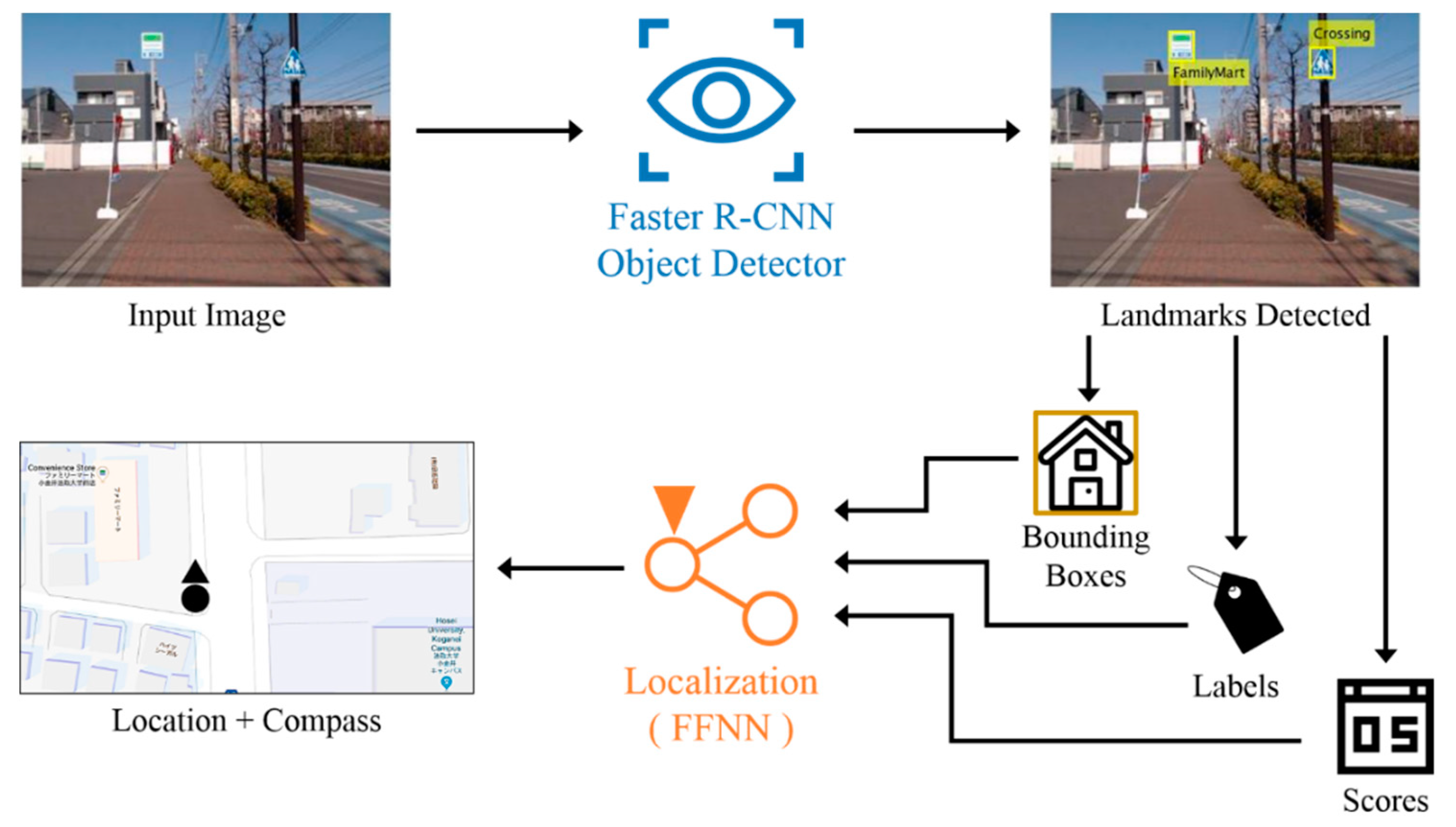
The overview structure of the Faster R-CNN based localization method is illustrated in
Figure 1. The Faster R-CNN based method is a two-step procedure. Faster R-CNN object detector and FFNN are two main components of the first outdoor localization method. During the robot navigation, Faster R-CNN detects landmarks in the camera captured image. This landmark detection process generates three types of answers for each instance of the detected landmarks, which are bounding box, label and score. Bounding box contains the position and size of the detected landmark in the input image. Label indicates the class name of the detected landmark. Score refers to an objectness score, which measure membership of the bounding box to classes of landmarks or background [
17]. The components of each detected landmark are then sent to FFNN for localization. The localization part uses detected landmarks from the Faster R-CNN to localize the robot in the real-world environment. FFNN for localization utilizes bounding boxes and labels of detected landmarks to generate geolocation data as the result of the localization system. The generated geolocation data includes location coordinates and compass orientation, in which location coordinates are in the form of latitude and longitude angles, and orientation is in the form of magnetic-referenced compass orientation.
Further details on two main components of the Faster R-CNN-based localization method are described in the following subsections.
2.1.1. Faster R-CNN for Landmark Detection
Landmark detection is the first process of our Faster R-CNN localization method. We employ the standard version of the Faster R-CNN object detector for landmark detection tasks. Typically, Faster R-CNN comprises two modules, i.e., Fast R-CNN object detector and region proposal network (RPN). The structure of Fast R-CNN object detector contains several convolutional and max pooling layers, a region of interest (RoI) pooling layer, and a sequence of fully connected layers. In Fast R-CNN, a set of convolutional layers and max pooling layers constructs a convolutional feature map from an entire input image. RoI pooling extracts a fixed-length feature vector from the feature map at each region, which is used as input of the Fast R-CNN. At final points of the Fast R-CNN, fully connected layers estimate classes of feature vectors from RoI pooling and refine result bounding boxes from these feature vectors [
18]. The RPN is a deep fully convolutional neural network that shares full-image convolutional features with the detection network, Fast R-CNN. RPN proposes high-quality regions to the Fast R-CNN module. In addition, it helps guiding the Fast R-CNN over locations of objects in the captured image [
17].
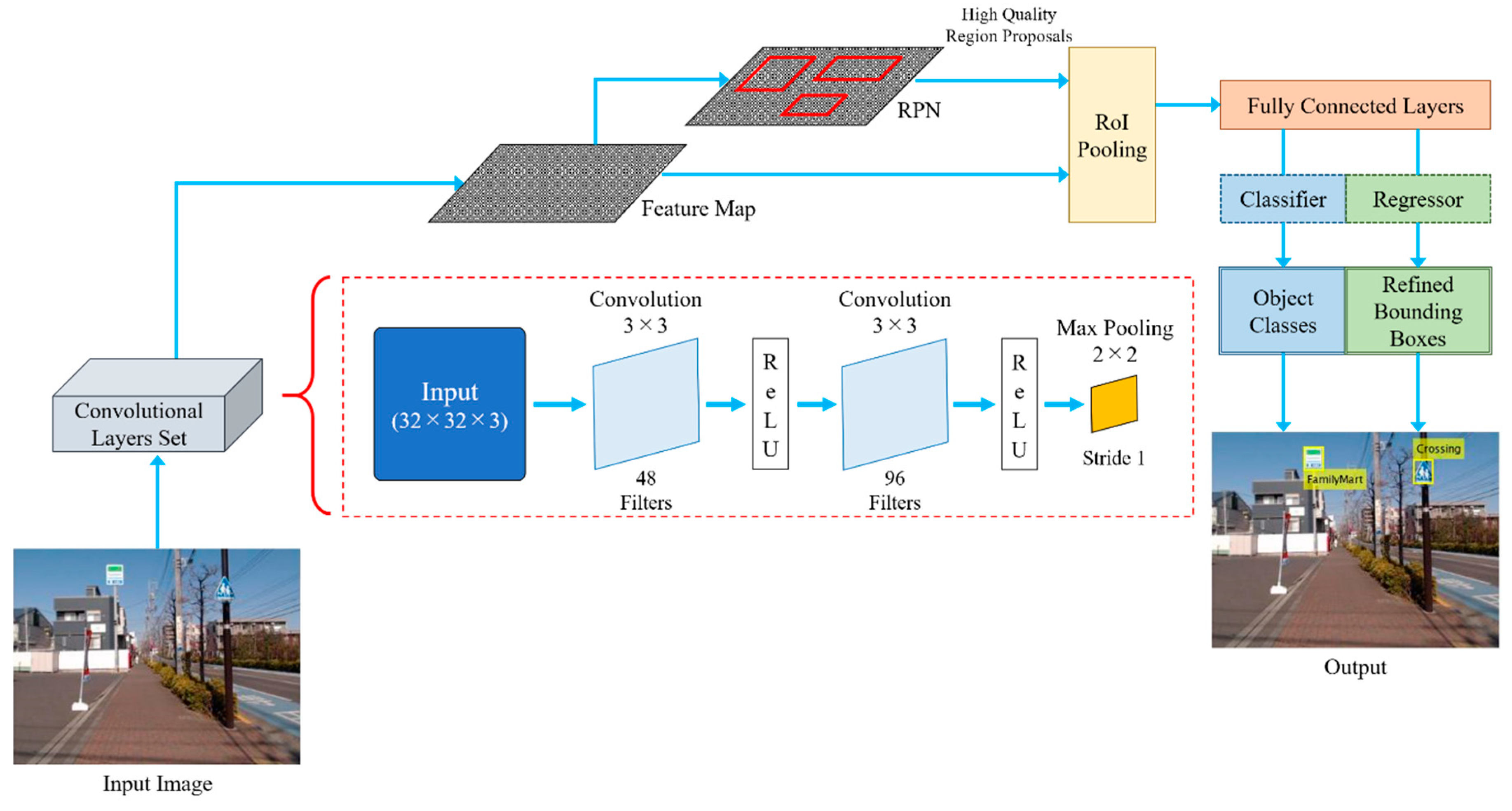
Architecture of the implemented standard Faster R-CNN is shown in
Figure 2. The whole input image is processed through the set of convolutional and max pooling layers of the CNN to generate a convolutional feature map. The feature map is then input to RPN to generate a set of rectangular region proposals. Since the feature map is shared across RPN and the detection network, the generated feature map is also input to the RoI pooling layer. This is used to extract fixed-length feature vectors, with help of region proposals generated from the RPN. Extracted feature vectors from the RoI pooling layer are then processed through a series of fully connected layers to estimate classes of each feature vector through classifiers and refine result region proposals form the feature vectors through regression process. Thus, refined and classified region proposals, or bounding boxes are generated from Faster R-CNN.
The structure of CNN used in our Faster R-CNN is also shown in
Figure 2. As mentioned earlier in this subsection, the set of convolutional layers of the CNN analyzes the whole input image to construct a convolutional feature map. As the size of the smallest landmarks in the utilized dataset is nearly 32 × 32 pixels, the input size is set to 32 × 32 × 3, where the last 3 is for three color channels: red, green and blue. The set of convolutional layers contains two, two-dimensional convolutional layers, with a rectified linear unit (ReLU) attached after each convolutional layer. The set also includes one max pooling layer for down-sampling purposes. Each convolutional layer employs a 3 × 3 filter and has the stride settings of 1 pixel for both horizontal and vertical strides. The number of filters in the first convolutional layer is 48, while 96 filters are used for the second convolutional layer. The max pooling layer is placed at the end of the layers set, in which the pooling size is 2 × 2 and the stride settings is 1 pixel for both horizontal and vertical strides. This small pooling size is applied to prevent premature down-sampling of the input image, which may cause the loss of features in the result feature map.
Training of the Faster R-CNN consists of the following four steps: Step 1—RPN training; Step 2—Fast R-CNN training using region proposals from Step 1; Step 3—RPN re-training using the weight sharing with the Fast R-CNN for fine-tuning the RPN; and Step 4—Fast R-CNN re-training using the updated RPN. These steps are the same as the original Faster R-CNN training [
17]. The training uses the whole images as input, and the labeled bounding boxes as the target. Training continues for 20 epochs, with 1 × 10
−4 initial learning rate.
2.1.2. Feedforward Neural Network for Localization
The localization part generates the robot location using bounding boxes and labels of detected landmarks from the Faster R-CNN. Since the bounding boxes and labels are generated through the features in an image during the detection process in Faster R-CNN, bounding boxes of detected landmarks are arranged according to labels of landmark classes without further processing. The localization part of the Faster R-CNN method has a single FFNN as its core component, which uses arranged bounding boxes as input. The output units are location coordinates and magnetic compass orientation.
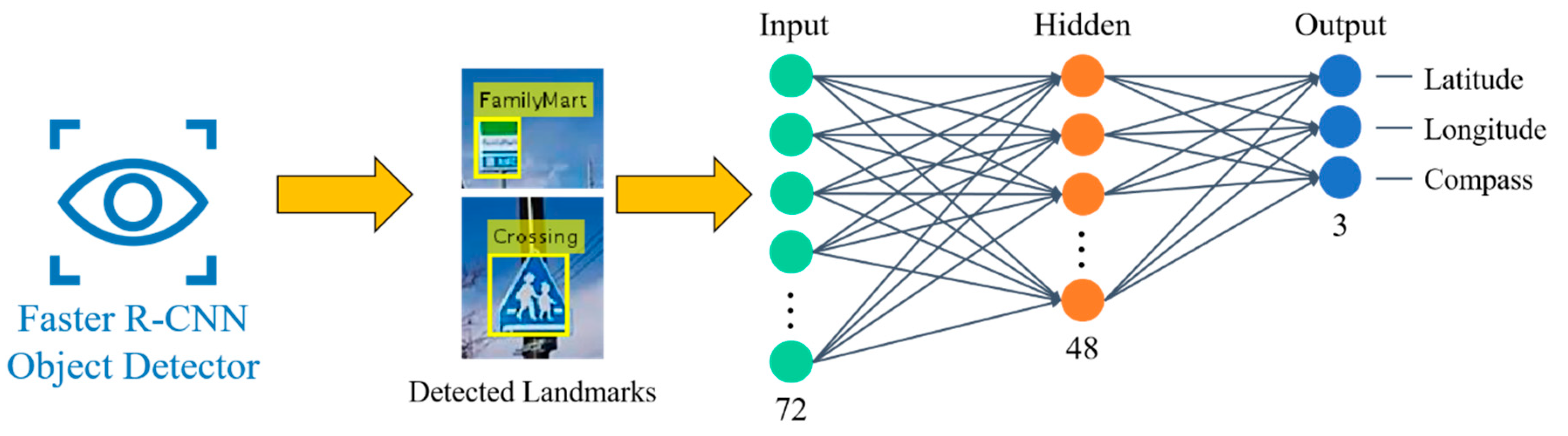
The implemented FFNN consists of 72 input neurons, 48 hidden neurons and three output neurons, as shown in
Figure 3. The 72 inputs are slots of bounding box elements of detected landmarks. Each bounding box contains four elements for positions and sizes of the box. We have limited the number of landmark classes to nine due the number of landmark classes in the experiments. Further details of nine landmark classes will be given in
Section 3. Each class has the limitation of maximum of two detection instances. For example, if there are three ‘Crossing’ landmarks detected, two instances with the highest objectness scores will be used for localization. This results in the total of 72 (9 × 2 × 4) input neurons. Default value of input neurons is zero if there is no detected instance for each slot of landmarks. The three output neurons correspond to latitude, longitude and compass. The number of hidden neurons, however, are acquired from trial-and-error tests. Activation function of FFNN neurons is the symmetric saturating linear transfer function.
Training of FFNN for localization utilizes labeled bounding boxes and geolocation data for training, with Bayesian regularization as the training algorithm. Bounding boxes are arranged according to the labels attached to boxes. Elements of arranged bounding boxes are used as the input of the training data. Geolocation data which includes latitude angles, longitude angles, and magnetic compass orientations, are used as the target training data.
2.2. CNN Localization
Convolutional neural network (CNN) is one type of deep neural networks that is suitable for two-dimensional array implementations, such as images. Typically, CNNs are applied for object detection and recognition purposes, in which final parts of CNNs mostly employ layers for classification. For instance, Softmax classifier. However, in our CNN localization method, CNN is used to directly determine the proper geolocation data from the image and its features within. The implemented CNN for localization has its final parts replaced with regressors instead of classifiers. Consequently, our CNN determines the geolocation data through regression output, instead of classification. Similar to the Faster R-CNN localization, the camera image is used as input for the CNN localization, where the whole input image is processed through all layers of the CNN. The result of our CNN localization method is the geolocation data, which consists of latitude angle, longitude angle, and magnetic compass orientation, the same as the Faster R-CNN localization results.
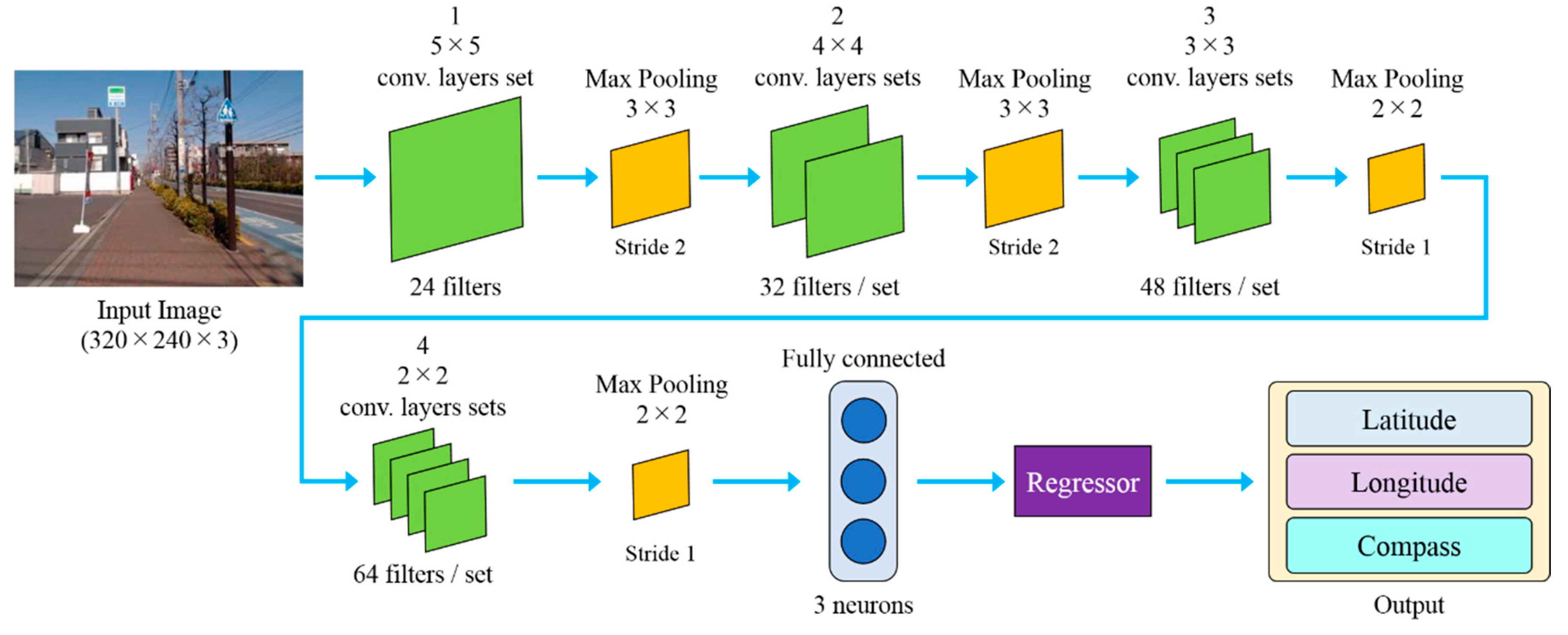
Design of the implemented CNN is shown in
Figure 4. The best architecture is determined by trial-and-error method and the combination from different CNN examples and principles available [
24]. The CNN for localization comprises 37 layers in total. The input layer of the CNN has the size of 320 × 240 × 3 (320 pixels width, 240 pixels height and three color channels: red, green and blue). There are 10 sets of convolutional layers, batch normalization and ReLU included within 37 layers of the CNN, where convolutional layer, batch normalization and ReLU are displayed together as one green layer in the diagram. There are different sizes and different amounts of filters among the implemented convolutional layers. The earliest convolutional layer employs the largest filter size of 5 × 5, while the filter size is decreasing as the network continues deeper, to the last convolutional layers which apply the filter size of 2 × 2. On the contrary, the number of filters begins with a small number of 24 filters in the first convolutional layer. The number of filters in each convolutional layer set increases as the network progresses deeper, to the amount of 64 filters in last layers. We employ four max pooling layers at the size of 3 × 3, 3 × 3, 2 × 2, and 2 × 2, with the stride settings as 2, 2, 1, and 1 respectively. Final parts of the CNN for localization consist of a fully connected layer and the regressor. Since the localization is determined based on latitude, longitude, and compass orientation, only three neurons are employed in the fully connected layer of the CNN.
The implemented CNN training employs a whole captured image as the input, and geolocation data as the training target. Setup for CNN training includes 48 training epochs, batch size of 64 and 1 × 10⁻⁶ initial learning rate. The learning rate decreases at the rate of 0.1 every 20 epochs.
3. Experimental Results
Experiments of our localization methods start from the dataset construction. The geotagged image dataset is constructed to provide the data for both training and testing of our localization methods. In total we created a dataset of 1625 data, which is relatively small compared to most of deep learning implementations. From 1625 sets of data in the dataset, 1198 sets were randomly selected for the training process, while the remaining 427 sets were used to test the performance. Reducing the amount of training data is a very important research issue in the deep learning community. Our developed localization methods were tested in terms of localization accuracy. The Faster R-CNN localization method was also tested in terms of landmark detection accuracy.
3.1. Geotagged Image Dataset
Similar to other deep learning systems, the Faster R-CNN, FFNN and CNN employed in our localization methods require data for both training and test. The dataset was constructed from 1625 images in the form of JPEG color images at the size of 320 × 240 pixels. Each image was tagged with the corresponding geolocation data, including location coordinates, in the form of latitude and longitude angles, and compass orientation. Geotagged images were labeled with bounding boxes of landmarks in each image. In summary, one set of data consists of an image, latitude angle, longitude angle, magnetic compass orientation, bounding boxes of landmarks in the image and labels of landmarks for bounding boxes.
The training set, which includes randomly-selected 1198 sets of data, was employed for training all components of both Faster R-CNN and CNN localization methods. Faster R-CNN for landmark detection used whole images and labeled bounding boxes of landmarks for training. FFNN for localization in the Faster R-CNN localization method used labeled bounding boxes and corresponding geolocation data for training. CNN for localization used whole images and corresponding geolocation data for training.
Experimental results of proposed localization methods were generated with the data in test set as the input of both localization methods. The landmark detection tested the Faster R-CNN performance with all images in the test set as inputs, and compared the results with corresponding bounding boxes of test images. The proposed localization methods were tested using all images in the test set as inputs. The results from both localization methods were evaluated by comparing with corresponding geolocation data of each test image.
3.1.1. Data Gathering
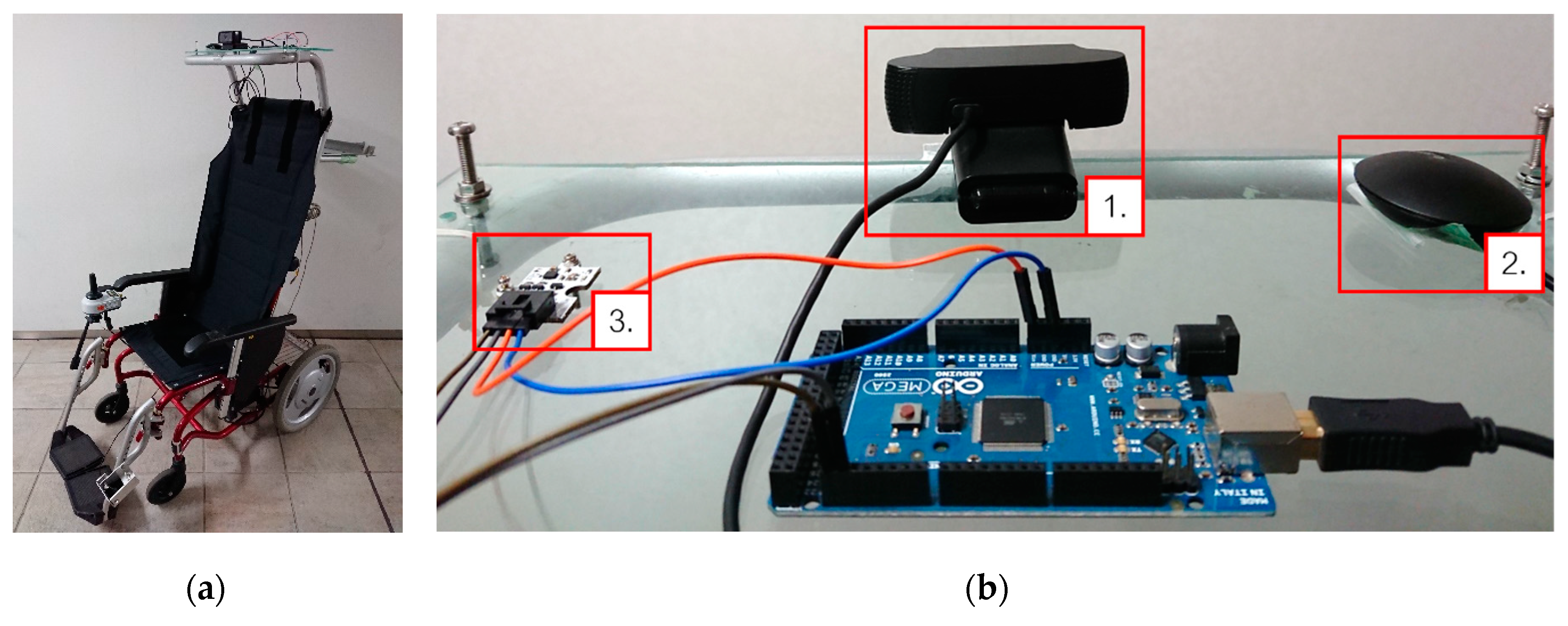
Geotagged images in the dataset were taken by a wheelchair robot equipped with camera, GPS receiver and compass sensor (
Figure 5). The wheelchair robot is 55 cm in width, 120 cm in length and 140 cm in height. Sensors for data gathering were attached above the seat. We used a Logitech C920 HD (Logitech, Lausanne, Switzerland) as the robot camera, BU-353S4 (GlobalSat, Taipei, Taiwan ) as the GPS receiver and an Octopus 3-axis digital compass sensor. All images in the dataset were taken from the area near Koganei campus of Hosei University, Japan. Two areas were selected for robot localization in outdoor environments, as shown in
Figure 6. The length and width of area 1 is 70 and 30 m, respectively. Area 2 is 75 m in length and 30 m wide. The two areas for experiments were in a distance of 250 m from each other. There are different types of landmarks available in each area, which distinguished one experimental area from the another.
During data gathering, the robot was pushed by a human, and images were taken manually. Each time an image was taken, the corresponding geolocation data was tagged to the image automatically. The tagged geolocation data includes location coordinates and compass orientation. Location coordinates were received from the GPS receiver in the form of a GGA message. Latitude and longitude information inside the GGA message was extracted and tagged to the image. Compass orientation was received from the compass sensor, converted to magnetic compass orientation, before being tagged to the image. We collected the data in different weather conditions in order to increase the robustness of the proposed algorithms.
3.1.2. Image Labeling
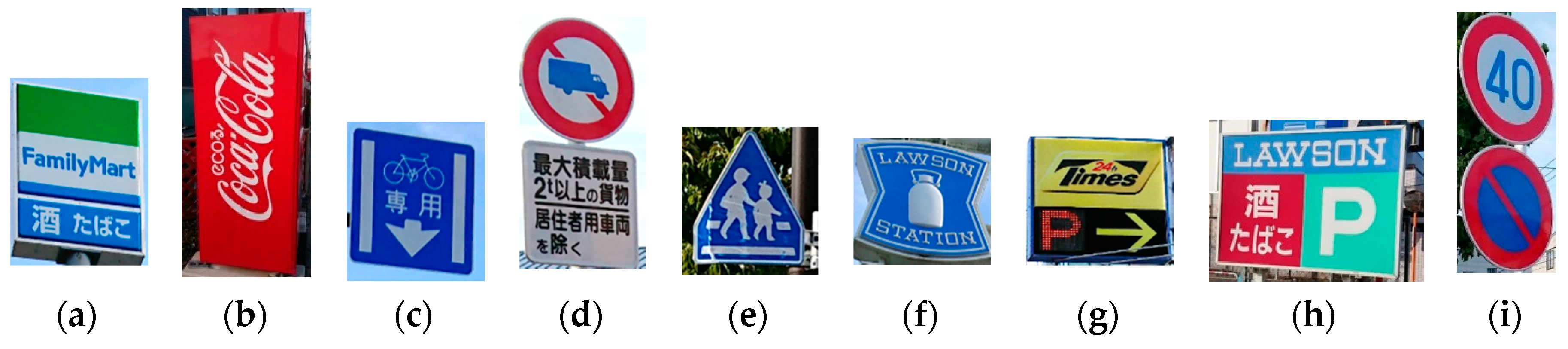
All gathered images in the dataset were hand-labeled with bounding boxes of landmarks in images. Nine types of landmarks were utilized for robot localization: ‘FamilyMart’, ‘CocaCola’, ‘BicycleLane’, ‘NoTruck’, ‘Crossing’, ‘Lawson’, ‘TimesParking’, ‘LawsonParking’, and ‘RoadSign 1’.
Figure 7 shows pictures of these nine landmarks in the area of experiments. Each bounding box is in the form of a vector with four member elements, which contains horizontal and vertical position coordinates of the top-left corner, width, and height of the bounding box in the image. Unit of position coordinates, width, and height of the bounding box is determined by the number of pixels. Horizontal and vertical position coordinates are referenced from top-left corner of the image. For example, a bounding box that has a vector of {10, 20, 56, 72} has its top-left corner at the pixel number 10 horizontally and 20 vertically, and the width and height of the box are 56 and 72 pixels, respectively.
3.2. Detection Experiments
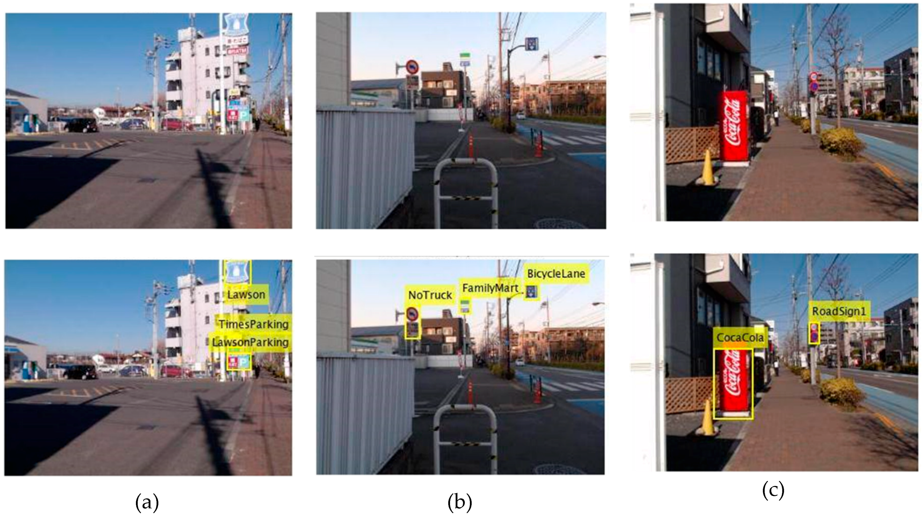
The goal of the landmark detection experiments was to evaluate the performance of the Faster R-CNN, since the localization part is strongly related with the landmark detection. All 427 images in the test set were processed through the Faster R-CNN, and embedded with bounding boxes and labels of landmarks detected by Faster R-CNN. Evaluation of detection results includes the qualitative and quantitative tests.
The qualitative evaluation was done by analyzing the detection results through human eyes. Some of detection results from the Faster R-CNN on images in the test set are shown in
Figure 8. Most of generated bounding boxes are placed well on detected landmarks with proper positions and sizes. Labels attached to the boxes correspond to the classes of landmarks shown in
Figure 7. However, some landmarks such as ‘CocaCola’ in
Figure 8c has its bounding box placed in the area of the actual landmark, but the box size did not match with the landmark size.
Mean Average Precision (mAP) was used for the quantitative evaluation in landmark detection experiments. mAP is considered to be the actual metric to measure the accuracy of object detectors. The mAP is the mean value of average precisions (AP) from all object classes. In this paper, we refer to this as landmark classes. AP is the average of maximum precisions at different recall values, in which both precision and recall can be calculated by the following equations:
where
P is the precision,
R is the recall,
TP is the amount of the correct bounding boxes comparing from detection and reference boxes in the dataset,
FP is the amount of missed or misplaced bounding boxes that appeared in detection results, and
FN is the amount of missed bounding boxes that did not appear in detection results, but existed in the reference dataset. The correct bounding boxes were measured from the ratio of intersection over union (IoU), which is the ratio between the intersection area and union area of bounding boxes, comparing detection results with reference data. The higher IoU ratio means less detection error allowance, which can also reduce the outcome of AP values. In this paper, the IoU of 0.5 and 0.7 were employed for measuring detection accuracy, similar to [
17] which used an IoU of 0.7. AP values of all landmark classes and the mean values (mAP) of 0.5 and 0.7 IoU ratio values are displayed in
Table 1.
From
Table 1, the mAP values are 0.8280 and 0.7375 for 0.5 and 0.7 IoU, respectively. This implies that the landmark detection accuracies of Faster R-CNN are 82.80% for 0.5 IoU and 73.75% for 0.7 IoU. Though mAP values were higher than 80% when IoU is 0.5, mAP decreased to around 70% as IoU increased to 0.7. This means landmarks could be detected but may not be precise or have high accuracy. Comparing to well-configured examples presented in [
19,
20,
21], the accuracy of our Faster R-CNN was moderately lower. This reduction in detection accuracy is the cause of a lower localization accuracy, as landmark detection results are required to generate localization results in the Faster R-CNN localization method.
3.3. Localization Experiments
The localization methods presented in this paper were implemented and evaluated in several localization experiments. All images in the test set were processed in the Faster R-CNN localization and CNN localization methods to generate localization results. In addition to two proposed localization methods, we added a CNN localization method based on the well-known CNN for classification called ‘AlexNet’ [
25]. We replaced the last layers of AlexNet with regression layers, similar to our second localization method. Training of the AlexNet was the same as our CNN in the second localization method. We employed AlexNet for localization as the reference for our second localization method, since there was no evaluation metric for testing our CNN design. Results from localization methods, including location coordinates in latitude and longitude, and compass orientations were then passed on to the evaluation.
Evaluation of localization results was done by calculating absolute errors and the distance between two points, the generated results and the reference geolocation data in the test dataset. Three absolute errors were considered in the experiments: mean, minimum and maximum absolute errors. The mean absolute error is calculated from the following equation:
where
MAE is the mean absolute error,
a is the result from localization,
b is the reference value in the test dataset, and
n is the amount of data in the test set, which was 427 in the experiments. The minimum and maximum absolute errors are the smallest and largest values in absolute errors.
The distances between two points were calculated from the location coordinates of the generated and reference data. We used the haversine formula to calculate distances from latitude and longitude of two points. The haversine formula is widely used in computer programming to determine the distance between two points on a great sphere, which commonly referred to as the Earth. The implemented haversine formula is as follows:
where
D is the distance between two points in kilometers,
r is the earth radius, which were applied as 6378.1 km [
26],
y1 is latitude of localization results in radius,
y2 is the reference latitude in radius,
x1 is longitude of localization results in radius, and
x2 is the reference longitude in radius.
In addition to absolute errors and distance errors, we also calculated the standard errors from localization results and distance errors. The standard errors were calculated to measure deviations of all results, in which the equation for standard errors can be described mathematically as;
where
SE is the standard error, σ is the standard deviation of the result, and
n is the amount of data, which was 427 for the test set.
Table 2 shows each localization error and the distances between the real and generated robot location. The mean, minimum, maximum and standard errors are calculated from absolute errors. Localization errors are the distances in meters calculated from location coordinates. It can be seen from
Table 2 that Faster R-CNN localization method outperforms both CNNs in terms of the location and distance errors. Mean absolute errors of latitude and longitude from the Faster R-CNN method are slightly lower than CNN methods, while minimum errors are also slightly lower in the case of Faster R-CNN. There are some differences in maximum errors of latitude and longitude for Faster R-CNN, CNN and the AlexNet. The AlexNet has lower errors than CNN localization, while the Faster R-CNN yields the least errors. These small errors in latitude and longitude cause significant differences in distance errors. The average distance error of the Faster R-CNN is 28 m which is less than half of the distance error of the CNN method (70 m). The reference AlexNet has an average distance error around 50 m. In the case of minimum errors, the distance error from Faster R-CNN is less than 1 m, while both CNNs for localization have distance errors around 3 m. On the maximum errors, the Faster R-CNN method has a distance error around 177 m, which is lower than CNN localization methods that have a distance error of 238 m. The reference AlexNet, however, gave the distance error of 322 m which is the highest among maximum distance errors.
However, performances of Faster R-CNN localization suffer a decline in compass accuracy. On average, compass orientations from the Faster R-CNN method can have the errors around 55°. Comparing to average errors of compass orientations from both CNNs, error from the Faster R-CNN is higher, in which the mean of orientations errors from CNN is only around 32° for our CNN and only 17° for AlexNet. In the best case with minimum errors, CNN methods also gave good results with the minimum compass error of around 0.2° from our CNN and 0.03° error from AlexNet, which are smaller than the minimum compass error from the Faster R-CNN method of 0.3°. For the worst case, all localization methods have the maximum compass errors near 180°, while our CNN gives the error of 152° which is the smallest among maximum compass errors.
The standard errors indicated that latitude and longitude coordinates resulted from all localization methods share the similar deviation, while the Faster R-CNN method has higher compass differences, and CNN methods have higher distance error differences in the results.
4. Conclusions
This paper proposed and tested two outdoor localization methods based on CNN and Faster R-CNN for mobile robots. The performance was evaluated in outdoor environment localization tasks. In addition, the AlexNet was implemented in order to compare the performance. Faster R-CNN localization method was also tested for landmark detection. Results from landmark detection yielded good performance, with more than 70% detection accuracy. Good detection performance of the Faster R-CNN led to good localization performance of the Faster R-CNN based method, with approximately less than 1 m distance error and less than 1° compass error in the best case. The CNN localization method also had good performance in the best case, with approximately 3 m location error and less than 1° compass error. The results from the average and worst cases pointed that the Faster R-CNN performs best among the tested approaches for localization tasks, while the performance declines for compass orientations.
However, there is still space to improve the localization results. The average location errors of proposed methods were relatively high, compared to the GPS that has approximately 4.9 m error [
7]. The orientation errors of our proposed methods were relatively high resulting in a poor performance compared with the reference AlexNet. Some possible causes of high orientation errors are as follows:
The development and experiments of the proposed localization methods were done with a small amount of data compared with other works that use more than half a million data.
There were less environmental variations during data gathering, despite attempts on gathering the data in multiple environmental conditions. Small environmental variations can be the cause of poor performance.
The performance of the Faster R-CNN localization method relied on landmark detection. If we improve the landmark detection, it will improve the performance of Faster R-CNN localization.
Despite the small amount of data, the proposed Faster R-CNN and CNN localization methods performed well for robot localization tasks. In the future we will focus on improving the performance of localization methods and implement them on the real robot. We will focus on continuous learning or transfer learning, in order to improve the performance without increasing the amount of data.


