Neural Network-Based Learning from Demonstration of an Autonomous Ground Robot

Abstract

This paper presents and experimentally validates a concept of end-to-end imitation learning for autonomous systems by using a composite architecture of convolutional neural network (ConvNet) and Long Short Term Memory (LSTM) neural network. In particular, a spatio-temporal deep neural network is developed, which learns to imitate the policy used by a human supervisor to drive a car-like robot in a maze environment. The spatial and temporal components of the imitation model are learned by using deep convolutional network and recurrent neural network architectures, respectively. The imitation model learns the policy of a human supervisor as a function of laser light detection and ranging (LIDAR) data, which is then used in real time to drive a robot in an autonomous fashion in a laboratory setting. The performance of the proposed model for imitation learning is compared with that of several other state-of-the-art methods, reported in the machine learning literature, for spatial and temporal modeling. The learned policy is implemented on a robot using a Nvidia Jetson TX2 board which, in turn, is validated on test tracks. The proposed spatio-temporal model outperforms several other off-the-shelf machine learning techniques to learn the policy.

1. Introduction

With explosive developments in machine learning and control techniques during the past few decades, mobile robots are taking an increasingly important role in modern society. Researchers in robotics have put a lot of emphasis on making mobile robots intelligent, which range from autonomous ground vehicles to smart unmanned aerial vehicles. Recently, in other domains (e.g., visual object recognition and natural language processing), deep learning [1] has set many impressive state-of-the-art benchmark results.

Conventionally, methods such as Simultaneous Localization and Mapping (SLAM) [2] have been shown to solve the problems of indoor mapping and navigation. While SLAM is focused on geometry, deep learning has been proven to be capable of handling perception problems effectively by using a convolutional neural network (ConvNet) [3,4]. Recently, there have been several attempts to use the tools of deep learning to complete the driving task for mobile autonomous vehicles. For example, Bojarski et al. [5] trained a ConvNet to map raw images from a camera directly to steering commands on a car. This system has learned how to drive on roads without lane markings and on highways without huge training data; however, a powerful and expensive computer is required for self-driving the car. In another example, Giusti et al. [6] trained a ConvNet to perceive forest trails with data collected from three-head-mounted cameras and implemented on a quadrotor aerial vehicle.

The concept of “end-to-end” learning has been recently introduced in the field of reinforcement learning (RL) [7]. It was popularized by Google’s seminal work on deep Q-network (DQN) [7]. A DQN agent would take raw pixel inputs from Atari video games, run it through a ConvNet and map the raw input directly to the discrete controller output. It is considered end-to-end training, because no human-engineered mid-level features are used throughout the learning process. DQN and its various improvements [8] have shown at least human-level performance in these tasks. To further develop these ideas and to use them in robotics and control applications, Zhu et al. [9] implemented deep reinforcement learning (RL) to find a target in an indoor environment using only visual inputs.

This paper presents a deep learning scheme by combining a convolutional neural network (ConvNet) [4] with a long short term memory (LSTM) [10] neural network for end-to-end learning, where the objective is to control and steer a mobile robot in a maze. The underlying algorithm has been successfully implemented on the robot for real-time inference-making and control. The concept is experimentally validated on a compact car-like autonomous robot platform called PSUbot. Using an Nvidia Jetson TX2 board as the onboard computer, PSUbot enables synchronized multi-sensor data acquisition for deep learning.

The problem of imitation learning (also known as learning from demonstration) [11,12] is addressed in this paper by PSUbot that learns how to navigate autonomously through different maze-like environments in a laboratory setting. Learning from demonstration (LfD) is a class of machine learning algorithms, where a teacher provides examples or trajectories for the robot to perform specified tasks [13]. In this context, an example is a sequence of observation-action pairs that are recorded during a demonstration. The core idea in LfD is to be able to learn the policy used by the expert supervisor directly. Unlike reinforcement learning (RL), LfD algorithms does not usually receive any reward for performing any action; rather it attempts to infer the policy being followed by the supervisor and using a classification or regression algorithm. In this paper, an LfD technique is presented, where the robot is shown demonstrations by teleoperation [14] as succinctly described below.

A dataset is first created by collecting the synchronized sensor information along with the steering command, which was created by a human expert during different experiments in various track scenarios. Then, an end-to-end policy is learned, which takes high-dimensional sensor data as the input and maps to the output directly to control the steering of the robot. Raw sensor data are first used to train a ConvNet, which is trained to reduce the classification error of the control inputs. The last fully connected layer of the ConvNet is then extracted and fed to an LSTM network which learns a temporal model for classification of the control inputs. The operation of the ConvNet can be viewed as an automatic feature extraction, which reduces the dimension of the input data; it is noted that no features are manually designed in this process. The next step is to incorporate memory into this system by using LSTM to increase the performance (e.g., accuracy) of the end-to-end network. These two networks are then combined to implement the trained model with Tensorflow [15] to perform real-time inference tasks and steer PSUbot in a test environment. The codes and data collected during the experiment are being made available here. The test system with on-board computer facilities, which is also presented here, can be used to develop and verify various learning and control algorithms for self-driving and autonomous systems in laboratory environments.

From the above perspectives, key contributions of the work reported in this paper are summarized below.

• Development of a compact robotic platform for real-time implementation of a variety of deep-neural-network-based concepts for data processing and control.
• Implementation and demonstration of a simplified concept of end-to-end imitation learning on a composite architecture of convolutional neural network (ConvNet) and Long Short Term Memory (LSTM) neural network.

The paper is organized in six sections, including the current section. Section 2 briefly introduces the architecture for ConvNet and LSTM neural networks. Section 3 introduces the hardware and software for PSUbot, and discusses the problem statement. Section 4 describes the proposed algorithm and associated technical details of the training and testing phases. Section 5 presents results of the proposed algorithm and compares them with those of various benchmarks. Section 6 summarizes contents of the paper and discusses a few topics of future research.

2. Background: Neural Network Architecture and Related Work

This section introduces the architectures for two major components of the proposed algorithm, namely ConvNet [3,4] and LSTM [10]. While there are many other excellent references (e.g., [16]), the underlying concepts of ConvNet and LSTM are very succinctly presented below for completeness of this paper. Besides, this section also briefly discusses other related work.

2.1. Convolutional Neural Networks

Convolutional neural network (ConvNet), first proposed in [3], is a class of neural networks, which uses convolution operations (instead of simple matrix multiplications) with the same neurons in a layer. In deep learning neural networks, the convolution is a discrete-domain operation, denoted by ∗, which is defined as ${(f\ast g)}_k\stackrel{▵}{=}{\sum }_{\ell }{f}_{\ell }{g}_{k-\ell }$, where the first argument f is the input and the second argument g is the kernel. It has been proven to work well with data that have a grid-like topology [17], such as images.

Traditional neural networks, which consist of fully connected layers, do not scale well to high-dimensional data (e.g., images), because each output unit is connected to each input unit by matrix multiplication. In contrast, ConvNets have sparse connections where each neuron is connected to only a local region of the input layer by the convolution operation. The dimension of the kernel g is usually much smaller than that of the input f. Since the convolution operation is applied to the same kernels at all positions of the input layer, the parameters needed to be stored are significantly reduced in the neural network, which increases its storage efficiency compared to that in fully-connected layers.

A typical ConvNet architecture includes pooling layers, which are applied after the nonlinear activation function that follows the convolutional layer. Pooling layers reduce the size of the representation and thus reduce the number of parameters and associated computations for the neural network. For example, the “Max Pooling” layer outputs the maximum value within a rectangular region. As a tool for downsampling, pooling layers make the representation invariant to minute input translations. Commonly used practical techniques (e.g., dropout [18] and batch normalization [19]) are used to improve the training accuracy and mitigate the overfitting problem of ConvNets.

2.2. Long Short-Term Memory Networks

Long Short-Term Memory (LSTM) neural networks [10] are a class of recurrent neural networks (RNNs) with a special architecture in the recurrent units. It is designed to overcome the long-term dependency problem [20], which is often encountered in traditional RNNs.

For an LSTM with an input $x_t$, an output $h_t$ and a cell state $C_t$, the “memory” is recorded in $C_t$ and it is a key component of the LSTM. Often used in the LSTM cells are the sigmoid function $\sigma \left(z\right)\stackrel{▵}{=}\frac{1}{1+exp(-z)}$ having a range of 0 to 1, and the hyperbolic tangent function $tanh\left(z\right)\stackrel{▵}{=}\frac{exp\left(z\right)-exp(-z)}{exp\left(z\right)+exp(-z)}$ having a range of −1 to 1.

The cell state ${\tilde{C}}_t$, its weightings $i_t$, and the forget gate [21] activations $f_t$ are computed as follows:

$$\begin{array}{ccc}\hfill i_t& =& \sigma \left(W_i{x}_t+U_i{h}_{t-1}+b_i\right),\hfill \end{array}$$

(1)

$$\begin{array}{ccc}\hfill {\tilde{C}}_t& =& tanh\left(W_c{x}_t+U_c{h}_{t-1}+b_c\right),\hfill \end{array}$$

(2)

$$\begin{array}{ccc}\hfill f_t& =& \sigma \left(W_f{x}_t+U_f{h}_{t-1}+b_f\right)\hfill \end{array}$$

(3)

where W’s and U’s are input and output weighting matrices, respectively, and the b’s represent the bias terms. With the operation ∘ defined to be elementwise multiplication, the update rule for cell state $C_t$ is computed as:

$$C_t=i_t\circ {\tilde{C}}_t+f_t\circ C_{t-1}$$

(4)

and the output $h_t$ is obtained as a weighted version of a nonlinear function of the cell state:

$$\begin{array}{ccc}\hfill o_t& =& \sigma (W_o{x}_t+U_o{h}_{t-1}+b_o),\hfill \end{array}$$

(5)

$$\begin{array}{ccc}\hfill h_t& =& o_t\circ tanh\left(C_t\right)\hfill \end{array}$$

(6)

Since Equations (1)–(3) and (5) depend only on $x_t$, $h_t$ and $h_{t-1}$, they can be efficiently computed in parallel with a graphics processing unit (GPU).

2.3. Related Work

Imitation learning trains a policy to make decisions from demonstrations. Main approaches for imitation learning are:

• Behavioral Cloning: It simply reduces the learning task to a supervised learning problem, and this technique was initially popularized by its application on helicopter acrobatics [22].
• Policy Learning with Iterative Demonstration: In practice, this sequential prediction problem of behavioral cloning sometimes leads to poor performance, and the DAgger (Dataset Aggregation) [11] algorithm is designed to improve the performance in an online iterative setting by training a stationary deterministic policy.
• Inverse reinforcement learning: The system attempts to learn a reward function given the demonstrations, and then use this reward function under the reinforcement learning framework to learn a policy. This approach was initially used in some simpler cases with given models [23], later extended to game-theoretic Inverse RL [24], maximum entropy Inverse RL [25] and more recently Deep Inverse RL [26] and Generative Adversarial Imitation Learning [27].

The proposed end-to-end learning method belongs to the first kind, i.e., behavioral cloning.

Imitation learning has also seen applications in many other fields, such as speech animation [28], improving over the teacher [29], structured prediction [30], safe learning for autonomous driving [31], learning with multiple objectives [32], one shot learning and meta learning [33,34], multi-agent learning [35,36], multi-modal learning [37], and hierarchical learning [38].

A combination of ConvNet and LSTM have been used in end-to-end learning for control of autonomous vehicles; however, existing methods may not be easily applicable to small-scale laboratory robots for real-time applications. For example, Chi et al. [39] proposed a network with Feature-Extracting Sub-network and Steering-Predicting Sub-network. In the first sub-network, a spatio-temporal convolution operator is used instead of matrix multiplications in standard LSTMs. It also introduces skip-connections into the architecture and employs a multi-task objective function. This method is computationally expensive, because a private cluster with 11 computing nodes has been used with 6 Titan X GPUs, which may not be feasible on actual autonomous vehicles. Another example is the work reported by Eraqi et al. [40] who also proposed a ConvNet-LSTM structure with a pre-trained ConvNet from Imagenet dataset; however, this concept have not been implemented on a real robot. Pan et al. [41] reported an imitation learning scheme by using an algorithmic expert with Model-Predictive Control and a simple ConvNet to learn the control policy. There have been some other work that combines ConvNet and LSTM for non-robotic applications. Examples include modeling cognitive events from electroencephalogram [42] and in sentiment analysis [43].

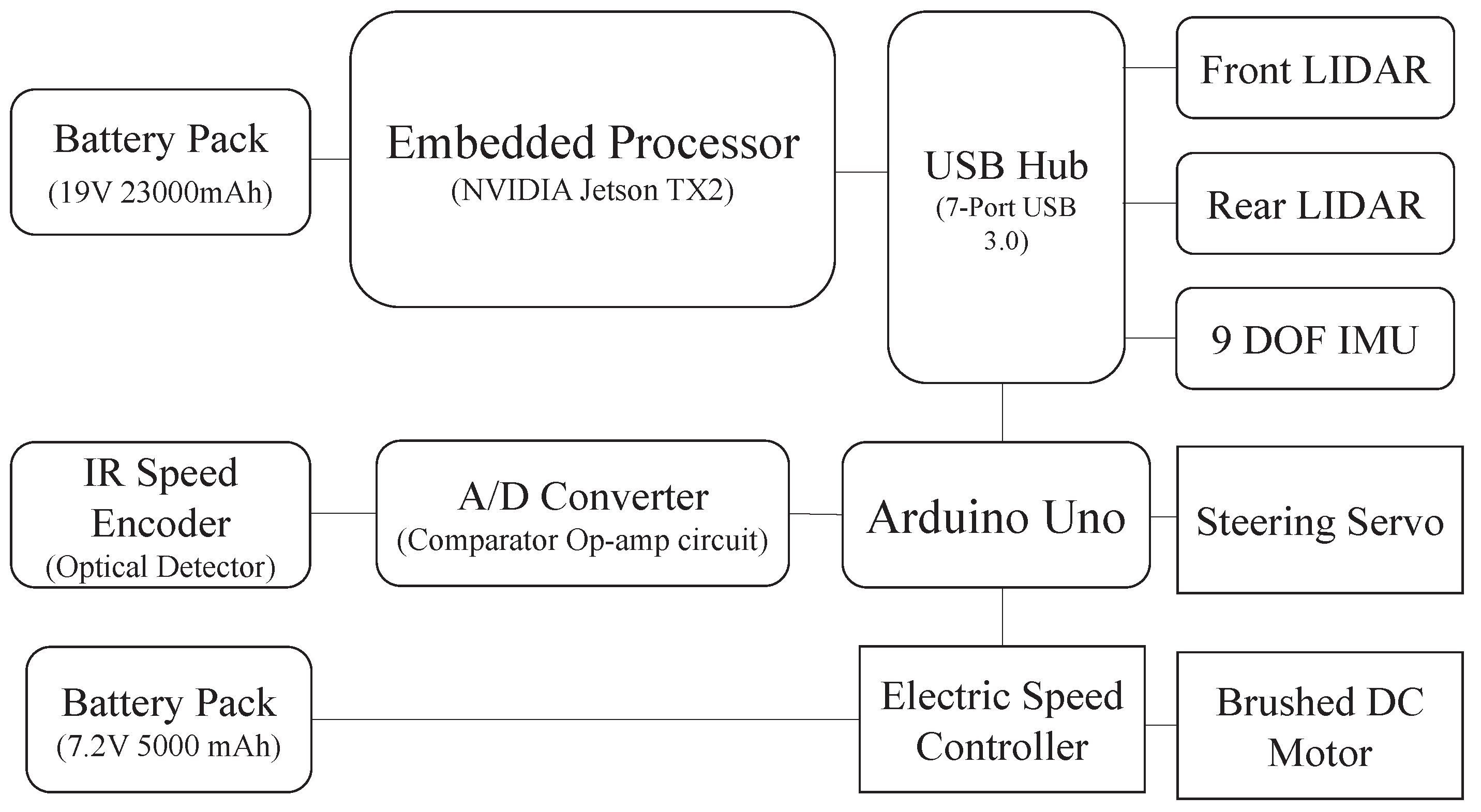
3. Platform Description

This section introduces the hardware and software used in the mobile robot platform, as well as the dataset for the subsequent learning and control applications.

3.1. Hardware Setup

Figure 1 shows a picture of the robot PSUbot used in the experimental validation, which is a 1/10 scale autonomous car platform built on a Tamiya RC TT02 Chassis with a set of components installed. Nvidia Jetson TX2 embedded computer is installed on the chassis of the robot as the main processor. The robot platform (ROS codes for the robot downloaded at https://goo.gl/EFcwxC) runs on an open-source software, called Robot Operating System (ROS) [44].

The TX2 platform has a built-in USB 3.0 port that receives data from multiple onboard sensors through a seven-port USB hub. The USB hub is connected with four individual components: two laser light detection and ranging (LIDAR) sensors, one inertial measurement unit 9-DOF-IMU, and an Arduino Uno. Figure 2 shows the connection diagram of these components to the platform Nvidia TX2 that has an onboard RGB camera that can also be used as a sensor in many tasks. A 19 V battery is used to supply power to the TX2 board, while a different 7.2 V battery pack is used as a power supply for the wheels.

Two Hokuyo URG-04LX LIDAR sensors are installed on the top layer of the robot, facing both front and back. Each LIDAR sensor has a ${180}^{\circ }$ scanning angle although they can have a maximum of ${240}^{\circ }$ measuring area. Therefore, the LIDAR sensors have a 360 degree view for target detection in the surrounding environment.

The Sparkfun 9-DOF-IMU consists of three sensors: accelerometer, gyroscope, and magnetometer. With all these three sensors, the IMU is able to measure and record the car motion, such as linear acceleration, angular rotation velocity, and magnetic field vector.

In order for TX2 to operate the car platform, an Arduino Uno is implemented onboard as a lower level microcontroller. The Arduino is used to connect the TX2 with the motor and the steering servo. It receives commands from the TX2 and sends corresponding Pulse-Width-Modulation (PWM) signals to the corresponding actuators. The proportional-integral-derivative (PID) control logic is applied to Arduino for speed control, where two optical detectors are installed inside the rear wheels as speedometers. The Arduino receives speed information transmitted from the optical detectors through an analog-to-digital converter (ADC) circuit mounted on top of the Arduino. This information is processed as sampled speed feedback for the PID controller. The TX2 has a built-in WIFI module that can communicate with a host computer to receive location information from a VICON indoor motion capture system.

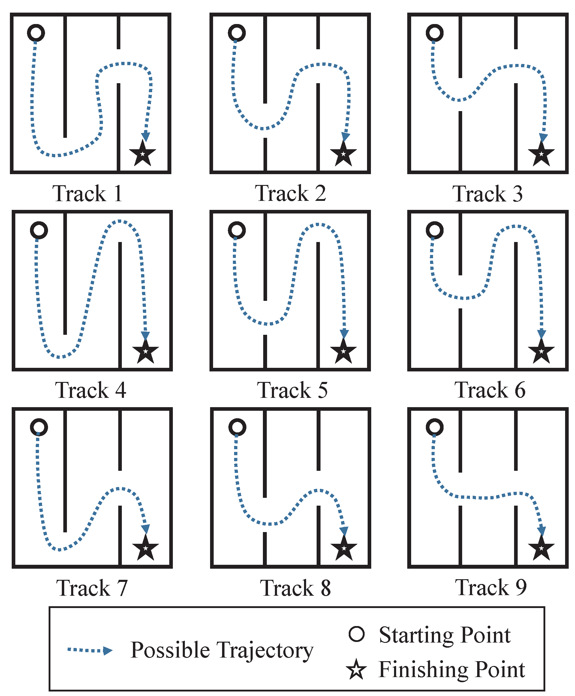
3.2. Description of Data Sets

Using PSUbot, data were collected from 9 different tracks that were set up in an approximately 5 m × 5 m indoor environment. Figure 3 shows configurations of all tracks. For each of these nine tracks, 10 runs are performed with the steering controlled by a human expert. The human expert operates a racing wheel which is connected to the same host system as in Section 3.1. The host system then maps the human expert’s steering command directly to PSUbot’s Arduino and controls the steering servo of the mobile robot in real-time.

Synchronized data have been collected and converted to JSON format for easy read and write, and these data are provided with this paper (The dataset downloaded at https://goo.gl/YTLemL). The data are synchronized at 10 Hz, which is the LIDAR’s scan frequency and also the lowest frequency of all sensors. The controller is also set to operate at 10 Hz to match the sensor inputs. In the experiments, the controller was set on the robot to output a discrete control command from seven possible values, with the lowest value meaning steering all the way to the left and highest value meaning steering all the way to the right. There are three different steering angles for both turning left and turning right, and one command for going straight.

The collected sensor data consisted of $3D$ angular velocity, linear acceleration and orientation with IMU. Front and rear LIDAR records the range information in meters of ${180}^{\circ }$ to the front and rear of the robot with an array of shape $512\times 1$ each. The resolution of the LIDAR sensor is approximately $\frac{{180}^{\circ }}{512}\approx {0.36}^{\circ }$. The absolute location of the robot with respect to the global coordinate system of the VICON motion capture system is also recorded in this dataset, which provides the trajectory of PSUbot.

4. Control Objectives and Proposed Algorithm

This section outlines the control objectives and presents the proposed architecture of the neural network for the task of steering PSUbot given sensor data inputs only. The detailed architecture for the proposed neural network structure is illustrated in Figure 4.

4.1. Control Objectives

The purpose of the task is to make a robot navigate in an indoor environment until it reaches the objective without any collisions. Correspondingly, the control objective for the machine learning algorithm, which drives this autonomous robot, can be set as minimizing the mean squared error (MSE) between the trajectory of the actual robot and the trajectories generated by human experts. If the autonomous robot can learn from the demonstrations of human experts and make decisions accordingly, it should be able to achieve similar levels of competence in this environment.

4.2. Algorithm Development

A deep neural network architecture is proposed to learn how to steer the mobile robot with the front LIDAR data as the only input, which is formulated as a supervised learning problem. As described in Section 3, the LIDAR sensor data is a $512\times 1$ array at each scan with a frequency of 10 Hz. A ConvNet is first used to perform feature extraction and dimension reduction for the input data. As shown in Figure 4a, the input layer is followed by a convolution layer of 32 filters of kernel size 3. With this convolution operation on 32 kernels, the data dimension is now $512\times 1\times 32$. The convolution layer is followed by a 1D max pooling layer of pooling size 4 and stride 4, where the dimension of the data is reduced from $512\times 1\times 32$ to $128\times 1\times 32$. This is a 1D pooling layer instead of the often used 2D pooling layers in many applications of images, because the second dimension of the input data is 1. A $20\%$ dropout is repeated, where batch normalization has been used before the (nonlinear) activation function ReLU (i.e., $f\left(x\right)\stackrel{▵}{=}max(x,0)$). The process is repeated for two more times with 64 and 128 convolution filters. Then, this structure is followed by a fully connected layer with $64\times 1$ output feature shape. The final output layer is of size $7\times 1$ because, in this case, there are 7 possible control commands for steering PSUbot.

The training of ConvNet is followed by the training of the LSTM as shown in Figure 4b. The input to the LSTM is the $64\times 1$ feature extracted before the final output layer of the ConvNet. Two LSTM layers are stacked together with the number of hidden states (i.e. the dimension of $h_t$ in Section 2.2) set to be 200. Then, these stacked LSTM layers are connected to a fully connected layer that outputs the $7\times 1$ control command. This control command is then directly mapped to the robot steering.

Justifications for the proposed deep learning neural network architecture, as a combination of ConvNet and LSTM, are delineated as follows:

• ConvNets are proven to be successful in many fields, including robotic imitation learning as described in Section 1. The properties of input sensor data in this application are similar to those of ConvNet; for example, the underlying data are high-dimensional and are arranged with spatial relationships.
• LSTM is capable of handling sequential data. Unlike many ConvNet applications (e.g., image classification) that make the assumption that the data are independent and identically distributed (iid), robotic sensor data are not. Therefore, LSTM takes the role of preserving past information (i.e., having memory), thus making this system more intelligent with enhanced accuracy.
• LSTM alone may not be very good for handling high-dimensional sensor data. To alleviate this difficulty, ConvNet is used here as a feature extraction tool to reduce data dimension as in Figure 4. By taking the layer just before the output layer in ConvNet and feeding it to the LSTM, this architecture takes advantage of the strengths of both ConvNet and LSTM. The procedure is used first to feed the raw data through the ConvNet and then to extract the features and feed them through the LSTM to obtain the output control command; this procedure is implemented on the robot for real-time inferencing and control.

The details of training and hyperparameter identification, used in the implementation, are presented in Section 5.

5. Results and Discussion

This section describes in detail the training and testing procedures with acquired data. In the experimental validation, the results of the proposed concept are compared with those of various standard machine learning tools.

5.1. Data Preprocessing and Hyperparameter Setting

Preprocessing is required before feeding the data into the neural network. The LIDAR sensor data may contain “NULL” entries when the laser does not reflect back, and this will cause problems to the numerical calculations in the neural network. Therefore, all “Null” entries in the input data are replaced with a numerical value of 10 (indicating that the range is 10 m at that angle, which is more than the range of the LIDAR and should be enough for this indoor environment.

Although the problem of online time series prediction with missing data have been traditionally addressed by model-based techniques (e.g., Kalman filtering (KF) and maximum likelihood (ML)), they are not apparently suitable for data preprocessing in this case, because of the following reasons:

• The plant dynamic model and measurement model for Kalman filtering are not available.
• The statistical assumptions on the error terms such as independence and Gaussian distribution for ML methods may not be satisfied.

It is argued in [45] that an online learning approach based on autoregressive (AR) models without these assumptions on the models generating the time series is more robust and works better. Neural networks have also been used to perform time series prediction without creating an underlying data generation model [46], and it has been shown to work better than AR models. Furthermore, unlike those reported in the literature, where the time series data are often one-dimensional, the input data in this experiment are high-dimensional with spatial relationships among adjacent data dimensions. Therefore, it is not computationally efficient to develop a data prediction model to handle the rare cases of missing data. Since the reason for “Null” data is clear here (due to sensor data being out of range), one may justify replacing the missing data with a numerical value. Besides this preprocessing, the control commands are remapped to 0∼7, with 0 being the leftmost steering angle, 7 being rightmost steering angle and the rest in between. This procedure is adopted to generate the output in the network training, and is implemented as follows: The input x here is the front LIDAR range information in meters as a $512\times 1$ vector, and the label y is the control commands a $7\times 1$ vector corresponding to the steering actions provided by the human expert.

During the ConvNet training phase, hyperparameters are set as follows: batch size $=256$, number of epochs $=200$, and number of batches per epoch $=100$. The Adam optimizer [47] with a learning rate $=0.001$ is used as the gradient descent algorithm.

For training the LSTM, hyperparameters are chosen such that number of time steps is 10 (i.e., inputs $x_t,x_{t-1},\cdots ,x_{t-9}$ into the LSTM), batch size $=400$ and number of epochs $=200$. The gradient descent optimizer Adam is used again here, but with a small modification—gradient clipping [48] with a value of 5 added to the optimizer to prevent exploding of the gradients in the recurrent neural network. In the test phase, dropout probabilities are set to 0.

5.2. Implementation

Figure 4 shows how the proposed architecture of deep neural network is implemented with Tensorflow, trained, and tested. The hyperparameters are set as those stated in Section 5.1. The implementation is performed on two different training set/test set split for comparison with various other machine learning algorithms [49] as seen in

Table 1. Results of using all ten runs from 8 tracks as training set, and all ten runs from the other 1 track as test set. Proposed method (ConvNet + LSTM) are compared with various machine learning methods using accuracy and root mean square error (RMSE0 as metrics respectively; the performance is deemed better for higher accuracy and lower lower RMSE.

Metrics	Training Set		Test Set
	Accuracy	RMSE	Accuracy	RMSE
Proposed Method	82.44%	0.7290	71.90%	1.2538
ConvNet Only	82.13%	0.8213	56.85%	1.9686
LSTM Only	65.06%	1.6753	49.64%	2.7885
KNN	81.42%	0.9470	59.62%	1.7454
SVM	69.29%	1.3648	63.69%	1.9417
Decision Tree	61.26%	1.8906	58.20%	1.7970
AdaBoost	69.50%	1.4305	58.70%	2.1268
Gaussian Process	91.90%	0.4472	66.33%	1.6396

that presents the results of the proposed deep neural network model versus various benchmark machine learning methods, using all 10 runs 8 tracks as the training set, and 1 track as the test set. Two different kinds of metrics are used to evaluate the results on both training set and test set, i.e., accuracy and root mean squared error (RMSE). Since the class label y is categorical and ranges from 0 to 7, it can be evaluated either as a classification problem with accuracy being a metric, or as a regression problem with RMSE being a metric.

For the ConvNet only method, the results are evaluated by using part (a) of the neural network in Figure 4. For LSTM only method, instead of feeding the ConvNet features into the LSTM as shown in Figure 4b, the $512\times 1$ raw data are directly fed into the LSTM layers. For the K-nearest-neighbor (KNN) algorithm implementation, a value of $K=5$ is used. For the support vector machine (SVM) algorithm, a grid search of parameters is performed and the best parameters are the following: kernel of radial basis function with parameters $\gamma =0.001$ and $C=1$. For AdaBoost algorithm, 10 decision trees of maximum depth = 5 and a learning rate of $0.2$ are used. For Gaussian process [50], a Matern kernel with parameter $\mu =2.5$ is used. The Gaussian process model is trained on 1000 samples randomly drawn from the training set, instead of the entire training set which will take too long to compute.

Table 2. Test results for using 8 runs in all 9 tracks as training set, and the other 2 runs in all 9 tracks as test set. Results of the proposed method (i.e., ConvNet + LSTM)) are compared with those of other machine learning methods using accuracy and RMSE as metrics respectively; higher accuracy and lower RMSE are desirable.

Metrics	Training Set		Test Set
	Accuracy	RMSE	Accuracy	RMSE
Proposed Method	81.21%	0.5628	71.09%	0.8626
ConvNet Only	82.81%	0.4627	68.81%	1.1724
LSTM Only	61.60%	1.8553	62.70%	1.7786
KNN	81.39%	0.9852	67.01%	1.3037
SVM	69.31%	1.3589	66.15%	1.4095
Decision Tree	63.80%	1.7226	61.44%	1.7557
AdaBoost	69.53%	1.4070	62.60%	1.6112
Gaussian Process	90.20%	0.5089	64.31%	1.7685

presents the results on a different training set/test set split, with 8 out of 10 runs recorded in all 9 tracks as the training set and the rest 2 runs in all 9 tracks as test set. For the other machine learning benchmarks, we use the same set of parameters as described above.

It is concluded from Table 1 and Table 2 that the proposed proposed method outperforms several existing machine learning methods. The results from Table 1 also indicate that the proposed method is much better at adapting to a new environment than other methods, while the results from Table 2 show that the proposed method is also better at learning the control strategy of a human expert in a known environment. Many of the other algorithms result in severe overfitting, which is quite common in imitation learning-type problems. Thus, the proposed method is superior to sole usage of ConvNet, because ConvNet is not capable of handling memory. Every decision made by ConvNet depends on only the current input, and the results show that although the data fit the training set well but they fail at the test set. The proposed method is also superior to to sole usage of LSTM, because it does not handle the high-dimensional input well. By combining the two neural networks (e.g., Covnet and LSTM) and using ConvNet as a feature extraction tool for LSTM, the proposed method performs much better than single usage of any one of them. For most other non-deep learning methods, they do not perform as well in this robotic learning scenario. The training can be done on PSUbot itself with its powerful yet low-cost and low-power consumption Nvidia TX2 embedded system, although the authors did use another desktop with dedicated GPU to train the deep neural network.

It is noted that the accuracy metric may not reflect the real capabilities of the proposed method due to the nature of the robotics application. Unlike many image classification tasks, where a misclassified label is considered wrong, here a misclassified label may not necessarily lead to a failure (e.g., crash). A possible scenario is that the human expert was steering at $y_{human}\left(t\right)=7$, but the proposed method generates an output of $y_{robot}\left(t\right)=6$. Accordingly, the robot will be turning at a smaller angle but it will still be able to navigate through the environment. In another scenario, the robot could have calculated a delayed control command; for example, if the outputs become $y_{robot}\left(t\right)=y_{human}(t+1)$, then it may still complete the task but the accuracy will suffer.

After loading the Tensorflow inference graph and resetting the learned deep neural network parameters, PSUbot is capable of making inferences for the robot motion in real time, where the actual time spent is insignificant in the time scale of the controller operating at 10 Hz. For implementation on a commercial-scale robot, a real-valued steering angle is calculated by taking expected values of the steering angles represented by respective classes. These expectations are calculated using the probability distribution before execution of the Softmax classifier in the LSTM output layer as seen in Figure 4. For example, if the probability distribution before executing the Softmax classifier is $[0.01,0.01,0.18,0.7,0.08,0.01,0.01]$, and the corresponding steering angles for the respective classes are $[-30°,-20°,-10°,0°,10°,20°,30°]$, the output steering angle would be the weighted average of $-1$° instead of exactly the steering angle of the output class 0°. Unlike image classification, where the desired output belongs to exactly one class, taking the expectation of the probability distribution makes sense in this robotic application, because of the specific way the output is mapped to a physical steering angle.

The learned controller has been implemented on PSUbot and tested in a laboratory setting. The code for implementing the real-time deep neural network controller is also included in the ROS package provided in Section 3. A video illustrating the learning results is provided with this paper (The video can be viewed at https://youtu.be/e5d34q0XCS4) to show how PSUbot successfully makes a turn without the human expert providing it with a control command, instead the proposed deep neural network is taking the real-time sensor inputs and making control decisions.

6. Conclusions

This paper has developed a deep learning technique that combines the theories of ConvNet and LSTM for steering a mobile robot with LIDAR sensor inputs. The data are collected on the PSUbot mobile robot platform, and the trained deep neural network controller has been implemented in a simplified and unambiguous manner on PSUbot for real-time decision and control. The proposed technique has been compared with several other state-of-the-art learning techniques and is shown to outperform all of them. The dataset for training and testing is also provided.

Although the proposed method is promising for intelligent and autonomous robots, much theoretical and experimental research is necessary before its real-life applications. The authors propose the following topics for future research.

• Implementing DAgger algorithm [11] on the current platform to enable interactive and iterative policy learning, and to reduce covariate shift and to make control policies robust.
• Inverse reinforcement learning for generating proper reward functions from observed agent behaviors. This should provide a better metric for evaluating the experimental results.
• Performance enhancement of deep learning-based inference-making in combination with traditional (e.g., model predictive) control techniques.
• Development of data preprocessing techniques for high-dimensional sensor time series with missing data. This machine learning technique is also applicable to problems of missing video data, and an efficient prediction algorithm has good potential for use in related fields.
• Quantitative performance evaluation in statistical settings. An example is quantitative performance evaluation using receiver operating characteristics for a trade-off between probability of successful task completion and probability of false alarms [51]. This will require extensive experimental work to create a large data base.

References

1. LeCun, Y.; Bengio, Y.; Hinton, G. Deep learning. Nature 2015, 521, 436–444. [Google Scholar] [CrossRef]
2. Durrant-Whyte, H.; Bailey, T. Simultaneous localization and mapping: Part I. IEEE Robot. Autom. Mag. 2006, 13, 99–110. [Google Scholar] [CrossRef]
3. LeCun, Y.; Boser, B.; Denker, J.S.; Henderson, D.; Howard, R.; Hubbard, W.; Jackel, L.D. Backpropagation applied to handwritten zip code recognition. Neural Comput. 1989, 1, 541–551. [Google Scholar] [CrossRef]
4. Krizhevsky, A.; Sutskever, I.; Hinton, G.E. Imagenet classification with deep convolutional neural networks. In Proceedings of the 2012 Neural Information Processing Systems, Stateline, NV, USA, 3–6 December 2012; pp. 1097–1105. [Google Scholar]
5. Bojarski, M.; Del Testa, D.; Dworakowski, D.; Firner, B.; Flepp, B.; Goyal, P.; Jackel, L.D.; Monfort, M.; Muller, U.; Zhang, J.; et al. End to end learning for self-driving cars. arXiv, 2016; arXiv:1604.07316. [Google Scholar]
6. Giusti, A.; Guzzi, J.; Cireşan, D.C.; He, F.L.; Rodríguez, J.P.; Fontana, F.; Faessler, M.; Forster, C.; Schmidhuber, J.; Di Caro, G.; et al. A machine learning approach to visual perception of forest trails for mobile robots. IEEE Robot. Autom. Lett. 2016, 1, 661–667. [Google Scholar] [CrossRef]
7. Mnih, V.; Kavukcuoglu, K.; Silver, D.; Rusu, A.A.; Veness, J.; Bellemare, M.G.; Graves, A.; Riedmiller, M.; Fidjeland, A.K.; Ostrovski, G.; et al. Human-level control through deep reinforcement learning. Nature 2015, 518, 529–533. [Google Scholar] [CrossRef]
8. Van Hasselt, H.; Guez, A.; Silver, D. Deep Reinforcement Learning with Double Q-Learning. In Proceedings of the Thirtieth AAAI Conference on Artificial Intelligence (AAAI-16), Phoenix, AZ, USA, 12–17 February 2016; pp. 2094–2100. [Google Scholar]
9. Zhu, Y.; Mottaghi, R.; Kolve, E.; Lim, J.J.; Gupta, A.; Li, F.-F.; Farhadi, A. Target-driven visual navigation in indoor scenes using deep reinforcement learning. In Proceedings of the IEEE International Conference on Robotics and Automation (ICRA), Singapore, 29 May–3 June 2017; pp. 3357–3364. [Google Scholar]
10. Hochreiter, S.; Schmidhuber, J. Long short-term memory. Neural Comput. 1997, 9, 1735–1780. [Google Scholar] [CrossRef] [PubMed]
11. Ross, S.; Gordon, G.; Bagnell, D. A Reduction of Imitation Learning and Structured Prediction to No-Regret Online Learning. In Proceedings of the 14th International Conference on Artificial Intelligence and Statistics (AISTATS), Fort Lauderdale, FL, USA, 11–13 April 2011; pp. 627–635. [Google Scholar]
12. Virani, N.; Jha, D.; Yuan, Z.; Sekhawat, I.; Ray, A. Imitation of Demonstrations using Bayesian Filtering with Nonparametric Data-Driven Models. J. Dyn. Syst. Meas. Control 2018, 140, 030906. [Google Scholar] [CrossRef]
13. Argall, B.D.; Chernova, S.; Veloso, M.; Browning, B. A survey of robot learning from demonstration. Robot. Auton. Syst. 2009, 57, 469–483. [Google Scholar] [CrossRef] [Green Version]
14. Ng, A.Y.; Coates, A.; Diel, M.; Ganapathi, V.; Schulte, J.; Tse, B.; Berger, E.; Liang, E. Autonomous inverted helicopter flight via reinforcement learning. In Experimental Robotics IX; Springer: Singapore, 2006; pp. 363–372. [Google Scholar]
15. Abadi, M.; Agarwal, A.; Barham, P.; Brevdo, E.; Chen, Z.; Citro, C.; Corrado, G.S.; Davis, A.; Dean, J.; Devin, M.; et al. Tensorflow: Large-scale machine learning on heterogeneous distributed systems. arXiv, 2016; arXiv:1603.04467. [Google Scholar]
16. Rozenberg, G.; Salomaa, A. Handbook of Formal Languages: Beyonds Words; Springer Science & Business Media: Berlin, Germany, 1997; Volume 3. [Google Scholar]
17. Goodfellow, I.; Bengio, Y.; Courville, A. Deep Learning; MIT Press: Cambridge, MA, USA, 2016; Available online: http://www.deeplearningbook.org (accessed on 18 November 2016).
18. Srivastava, N.; Hinton, G.E.; Krizhevsky, A.; Sutskever, I.; Salakhutdinov, R. Dropout: A simple way to prevent neural networks from overfitting. J. Mach. Learn. Res. 2014, 15, 1929–1958. [Google Scholar]
19. Ioffe, S.; Szegedy, C. Batch normalization: Accelerating deep network training by reducing internal covariate shift. In Proceedings of the International Conference on Machine Learning, Lille, France, 6–11 July 2015; pp. 448–456. [Google Scholar]
20. Bengio, Y.; Simard, P.; Frasconi, P. Learning long-term dependencies with gradient descent is difficult. IEEE Trans. Neural Netw. 1994, 5, 157–166. [Google Scholar] [CrossRef] [PubMed]
21. Gers, F.A.; Schmidhuber, J.; Cummins, F. Learning to forget: Continual prediction with LSTM. Neural Comput. 2000, 12, 2451–2471. [Google Scholar] [CrossRef]
22. Coates, A.; Abbeel, P.; Ng, A.Y. Learning for control from multiple demonstrations. In Proceedings of the 25th International Conference on Machine Learning, Helsinki, Finland, 5–9 July 2008; ACM: New York, NY, USA, 2008; pp. 144–151. [Google Scholar]
23. Abbeel, P.; Ng, A.Y. Apprenticeship learning via inverse reinforcement learning. In Proceedings of the Twenty-First International Conference on Machine Learning, Banff, AB, Canada, 4–8 July 2004; ACM: New York, NY, USA, 2004; p. 1. [Google Scholar] [Green Version]
24. Syed, U.; Schapire, R.E. A game-theoretic approach to apprenticeship learning. In Proceedings of the 2008 Neural Information Processing Systems, Vancouver, BC, Canada, 8–13 December 2008; pp. 1449–1456. [Google Scholar]
25. Ziebart, B.D.; Maas, A.L.; Bagnell, J.A.; Dey, A.K. Maximum entropy inverse reinforcement learning. In Proceedings of the Twenty-Third AAAI Conference on Artificial Intelligence (2008), Chicago, IL, USA, 13–17 July 2008; Volume 8, pp. 1433–1438. [Google Scholar]
26. Finn, C.; Levine, S.; Abbeel, P. Guided cost learning: Deep inverse optimal control via policy optimization. In Proceedings of the 33rd International Conference on Machine Learning, New York, NY, USA, 20–22 June 2016; pp. 49–58. [Google Scholar]
27. Ho, J.; Ermon, S. Generative adversarial imitation learning. In Proceedings of the 2006 Neural Information Processing Systems, Barcelona, Spain, 5–10 December 2016; pp. 4565–4573. [Google Scholar]
28. Taylor, S.; Kim, T.; Yue, Y.; Mahler, M.; Krahe, J.; Rodriguez, A.G.; Hodgins, J.; Matthews, I. A deep learning approach for generalized speech animation. ACM Trans. Graph. (TOG) 2017, 36, 93. [Google Scholar] [CrossRef]
29. Chang, K.W.; Krishnamurthy, A.; Agarwal, A.; Daume, H., III; Langford, J. Learning to search better than your teacher. arXiv, 2015; arXiv:1710.03804v3. [Google Scholar]
30. Ross, S.; Zhou, J.; Yue, Y.; Dey, D.; Bagnell, J.A. Learning policies for contextual submodular prediction. arXiv, 2013; arXiv:1305.2532. [Google Scholar]
31. Zhang, J.; Cho, K. Query-efficient imitation learning for end-to-end simulated driving. In Proceedings of the Thirty-First AAAI Conference on Artificial Intelligence, San Francisco, CA, USA, 4–9 February 2017. [Google Scholar]
32. Le, H.M.; Kang, A.; Yue, Y.; Carr, P. Smooth imitation learning for online sequence prediction. arXiv, 2016; arXiv:1606.00968. [Google Scholar]
33. Duan, Y.; Andrychowicz, M.; Stadie, B.; Ho, O.J.; Schneider, J.; Sutskever, I.; Abbeel, P.; Zaremba, W. One-shot imitation learning. In Proceedings of the 2017 Neural Information Processing Systems, Long Beach, CA, USA, 4–9 December 2017; pp. 1087–1098. [Google Scholar]
34. Finn, C.; Yu, T.; Zhang, T.; Abbeel, P.; Levine, S. One-shot visual imitation learning via meta-learning. arXiv, 2017; arXiv:1709.04905. [Google Scholar]
35. Le, H.M.; Yue, Y.; Carr, P.; Lucey, P. Coordinated multi-agent imitation learning. In Proceedings of the 34th International Conference on Machine Learning-Volume 70, Sydney, NSW, Australia, 6–11 August 2017; Microtome Publishing: Brookline, MA, USA, 2017; pp. 1995–2003. [Google Scholar]
36. Zhan, E.; Zheng, S.; Yue, Y.; Sha, L.; Lucey, P. Generative multi-agent behavioral cloning. arXiv, 2018; arXiv:1803.07612. [Google Scholar]
37. Li, Y.; Song, J.; Ermon, S. Infogail: Interpretable imitation learning from visual demonstrations. In Proceedings of the 2017 Neural Information Processing Systems, Long Beach, CA, USA, 4–9 December 2017; pp. 3812–3822. [Google Scholar]
38. Le, H.M.; Jiang, N.; Agarwal, A.; Dudík, M.; Yue, Y.; Daumé, H., III. Hierarchical imitation and reinforcement learning. arXiv, 2018; arXiv:1803.00590. [Google Scholar]
39. Chi, L.; Mu, Y. Deep steering: Learning end-to-end driving model from spatial and temporal visual cues. arXiv, 2017; arXiv:1708.03798. [Google Scholar]
40. Eraqi, H.M.; Moustafa, M.N.; Honer, J. End-to-end deep learning for steering autonomous vehicles considering temporal dependencies. arXiv, 2017; arXiv:1710.03804. [Google Scholar]
41. Pan, Y.; Cheng, C.A.; Saigol, K.; Lee, K.; Yan, X.; Theodorou, E.; Boots, B. Agile autonomous driving using end-to-end deep imitation learning. In Proceedings of the Robotics: Science and Systems, Pittsburgh, PA, USA, 8–11 June 2018. [Google Scholar]
42. Bashivan, P.; Rish, I.; Yeasin, M.; Codella, N. Learning representations from EEG with deep recurrent-convolutional neural networks. arXiv, 2015; arXiv:1511.06448. [Google Scholar]
43. Wang, J.; Yu, L.C.; Lai, K.R.; Zhang, X. Dimensional sentiment analysis using a regional CNN-LSTM model. In Proceedings of the 54th Annual Meeting of the Association for Computational Linguistics, Berlin, Germany, 7–12 August 2016; Volume 2, pp. 225–230. [Google Scholar]
44. Quigley, M.; Conley, K.; Gerkey, B.; Faust, J.; Foote, T.; Leibs, J.; Wheeler, R.; Ng, A.Y. ROS: An open-source Robot Operating System. In Proceedings of the ICRA 2009 Workshop on Open Source Software, Kobe, Japan, 17 May 2009; Volume 3, p. 5. [Google Scholar]
45. Anava, O.; Hazan, E.; Zeevi, A. Online time series prediction with missing data. In Proceedings of the 32nd International Conference on Machine Learning, Lille, France, 6–11 July 2015; pp. 2191–2199. [Google Scholar]
46. Hauser, M.; Fu, Y.; Phoha, S.; Ray, A. Neural Probabilistic Forecasting of Symbolic Sequences with Long Short-Term Memory. J. Dyn. Syst. Meas. Control 2018, 140, 084502. [Google Scholar] [CrossRef]
47. Kingma, D.; Ba, J. Adam: A method for stochastic optimization. arXiv, 2014; arXiv:1412.6980. [Google Scholar]
48. Pascanu, R.; Mikolov, T.; Bengio, Y. On the difficulty of training recurrent neural networks. In Proceedings of the 30th International Conference on Machine Learning, Atlanta, GA, USA, 16–21 June 2013; pp. 1310–1318. [Google Scholar]
49. Bishop, C. Pattern Analysis and Machine Learning; Springer: New York, NY, USA, 2006. [Google Scholar]
50. Rasmussen, C.E.; Williams, C.K. Gaussian Processes for Machine Learning; MIT Press: Cambridge, MA, USA, 2006; Volume 1. [Google Scholar]
51. Poor, H. An Introduction to Signal Detection and Estimation; Springer: New York, NY, USA, 1988. [Google Scholar]
Figure 1. Picture of the PSUbot platform.
Machines 07 00024 g001
Figure 2. Component interconnection diagram of PSUbot.
Machines 07 00024 g002
Figure 3. Schematics of the nine different tracks from which synchronized data have been collected. Dotted lines illustrate a typical robot trajectory.
Machines 07 00024 g003
Figure 4. Proposed deep neural network architecture: (a) ConvNet includes three convolutional layers, each followed by a max pooling layer with 20% dropout during training and batch normalization (BN). After flattening the final convolutional layer, a fully connected layer that produces 64 × 1 features is then connected to the output layer, which generate one out of seven classes. The 64 × 1 features are fed into (b) LSTM: 2 layers of LSTM are stacked together with 50 % dropout and 200 hidden states each, and then the output is directly mapped to the steering of the robot. Training is performed in two stages: firstly the ConvNet is trained; then parameters for this ConvNet are saved and frozen so that they consistently produce 64 × 1 features to be fed into the LSTM; then only the LSTM parameters are updated in next stages of training.
Machines 07 00024 g004