1. Introduction
In globally distributed supply chains, complex material flows between geographically widely separated suppliers and original equipment manufacturers (OEM) have to be coordinated [
1]. In the automotive industry, in particular, global sourcing and reduced vertical integration due to outsourcing result in the transport of large material volumes over long distances with potentially extreme environmental conditions [
2,
3,
4]. In combination with reduced safety stocks, these transports increase the susceptibility of the supply chains to disturbances [
5], and, consequently, increases supply chain risks, like inappropriate quality of the supply and poor logistics performance, e.g., late delivery [
6]. Such deviations potentially endanger the ability of the supply chain to meet customer expectations, so that success depends on the ability to prevent or at least immediately identify and resolve them [
7]. However, quality management procedures during transport are often not as sophisticated as during production [
8]. As a result, deviations are sometimes detected only at a late stage in the supply chain, resulting in costly compensation measures [
9,
10,
11].
Increasing digitalization in the context of Industry 4.0 offers the potential to increase the level of transparency in supply chains [
12]. The concepts of Industry 4.0 and Cyber-Physical Systems (CPS) are increasingly applied to logistics and supply chain management, as Logistics 4.0, and Cyber-Physical Logistics Systems (CPLS). A CPLS consists of CPS that are part of, or connected to logistic objects (like e.g., means of transport, or containers), or logistic processes and deal with the flow of information and goods in the value chain [
6].
Of particular interest in digital supply chain applications are sensor technologies. The ability to directly record physical data using sensors, and to evaluate and save the recorded data to globally distributed services via digital communication facilities is considered as integral to CPS in Industry 4.0 applications [
13].
Sensors can monitor a wide variety of ambient conditions, like temperature, humidity, mechanical stress levels on attached objects, and current characteristics of an object, such as location, speed, or direction. Combined to sensor networks, they can be used for continuous parameter sensing, event detection and identification [
14,
15]. As a result, sensor networks are considered as a suitable solution to provide the necessary information transparency in inter-organizational logistics and supply processes (e.g., the actual geographical position of the transports and their estimated arrival times, or the probability and level of the potential late deliveries) [
6,
8].
In previous work, we have proposed a sensor-based quality monitoring system for products during transport processes in automotive supply chains. This system combines a hardware infrastructure of mobile and stationary sensors and telematics units with a software infrastructure of sensor databases, data repositories, and digital services with the following characteristics [
16,
17]:
Mobile sensors are attached either directly to products, or to boxes, or pallets, used to harbor and store these products during transport. An example from the automotive industry are the universal load carrier (ULC) boxes, which fluctuate between suppliers and receivers of parts or components in automotive supply chains. This way, the sensors accompany the parts and components during transport and storage processes and measure relevant environmental parameters. The sensors should be capable of transferring their measurement data over a short distance (several dozen meters) wirelessly. It is important that the sensors are located close to the products that shall be monitored, and accompany them over the transport chain from beginning to end. In addition, they should be cost efficient enough to allow their application in larger numbers.
Telematics units, so called gateways, collect the wirelessly messaged measurement data from local sensors and transfer these data over large distances using standard telecommunication technology. As one such gateway can transfer the data of a larger number of sensors (up to a few hundred sensors), but are also more expensive in acquisition and operation, one gateway per transport unit (e.g., truck) or per transport container should be sufficient. In addition, the telematics units can house additional sensors, in particular, geolocation devices, like the Global Positioning System (GPS).
The sensor measurement data transferred by the gateways is stored in a central sensor database, which forms the data component of a software cloud platform.
In addition, digital services are hosted on such a cloud platform. These digital services perform operations on the collected sensor data. This includes the analysis of the sensor data to determine (potential) quality defects from the data and in such an event, to alert the relevant stakeholders in the supply chain, and propose corrective measures.
Occurrences of (potential) quality defects constitute critical events, which have to be communicated to processing applications of the various supply chain parties. Alerting companies to (critical) events, so that measures against those events can be taken proactively, is the task of Supply Chain Event Management (SCEM). Critical events are any unplanned changes in supply lines or generally critical exceptions in time [
7]. Quality related events are events that take into account (changes in) the quality state of the objects. Sensor measurements that are unusual or fall outside certain predetermined boundaries may point to changes in the surrounding of transport goods that affect the quality of the goods and thus constitute quality related (critical) events. The supply chain parties then can react to these events according to their own procedures. We have proposed to use the Electronic Product Code Information System (EPCIS) standard as an instrument to communicate such events. EPCIS is a standard that was developed and marketed by international non-profit organization GS1 for sharing event related data. Typically, it refers to the identification of certain physical objects at a certain time and place and within a certain context [
18]. As the EPCIS standard in its current version does not include data structures to express and communicate sensor data, we also have proposed proper extensions of the standard.
Our basic approach and some of its technical details have already been described in [
16,
17]. This article focusses on two particular aspects of using such a monitoring system to integrate sensor location and quality data into transport processes in automotive supply chains: First, we compile the environmental influence parameters that should be monitored during transport processes in automotive supply chains. In relation to metrological applications, it is important to exert systematic considerations concerning the planning, execution, and evaluation of measurements [
19]. The identification of the relevant measurement parameters constitutes an important aspect of the planning process of the metrological application. In this, we proceed from general environmental influences or conditions in transport processes and their cause-effect-relationships with critical failure mechanisms relevant to automotive product groups to establishing critical failure mechanisms of individual automotive products and components from product data sheets.
Second, the paper evaluates the potential effects of sensor-based quality data for supply chain performance. We use a discrete-event simulation model to study an exemplary automotive supply chain to investigate how the use of real-time quality status data for the supplied goods can influence supply chain control decisions and what impact on logistic performance it yields.
The structure of this paper is as follows:
Section 2 reviews related work, for example from cold chain logistics in the food or pharma industries.
Section 3 describes the relations between environmental influences and quality defects of automotive products.
Section 4 outlines the simulation study and its results.
Section 5 provides a discussion of the results of
Section 3 and
Section 4. Conclusions and ongoing work are outlined in
Section 6. An
appendix provides additional tables detailing aspects of
Section 3.
2. Related Work
We cluster the related work into two groups. As a first group, a large body of work on product monitoring in supply chains using sensor systems exists for cold chains in the food industry, where factors, like temperature and humidity, are of foremost importance to product quality and expiration dates of perishable products. The second group relates to research publications covering the use of sensors for quality monitoring within transport processes of manufacturing industry supply chains. Here, we have found less publication.
In the first group of publications, Woo et al. [
20] have proposed a data model expressing temporal relationships between logistic objects passing at certain locations and sensors installed at these locations. A location may have more than one sensor for reading not only the radio frequency identification (RFID) data but also measuring environmental data. A temporal data entity stores the sensor data obtained when a logistics object passes through the sensor and is connected to the logistic objects to which the sensor reading applies. Hartley has examined the temperature control of wild animal meat in a global supply chain between New Zealand and Germany, using RFID and EPCIS [
21]. Kang and Lee propose a sensor integration architecture for cold chain management, where sensor data, such as temperature and humidity, are traced along with RFID based information [
22]. Kassahun et al. describe a reference architecture that enables chain-wide transparency in meat supply chains, making use of the EPCIS standard and cloud-based services [
23]. Thakur and Forås have evaluated the functionality of an online system for temperature monitoring in a cold meat chain. They use EPCIS for the communication of temperature data [
24]. The concept of virtual food supply chains has been analyzed from an Internet of Things perspective for the food industry by Verdouw et al. [
25]. In addition, the authors describe an implementation architecture, which is based on the cloud-based platform FIspace. Tamplin has published an approach for integrating predictive models and sensors to manage food stability in supply chains. His publication describes developments in predictive models designed for supply chain management of food products (like oysters and beef), as well as advances in environmental sensors [
26].
Applying sensor data to supply chain management has been investigated in the DynahMat project by Jevinger et al. One result was that it is crucial to measure temperature close to the freight using multiple distributed sensor nodes, instead of just thermometer per container. The DynahMat project also discusses dynamic pricing based on sensor data [
27,
28,
29].
Hertog et al. have published a study on how to derive the product quality of perishable food products, like e.g., strawberries, from sensor data [
30]. To set up a statistical control model, they define product specific critical tolerance levels of carbon dioxide, oxygen, temperature, ethylene, and relative humidity, which should not be exceeded. The authors state that above and below these tolerance levels, product damage will occur. Accidental occurrences of values outside these warning levels do not lead to significant decay in product quality, however, if these conditions occur more often or for longer time, the quality will be affected. Therefore they define a maximum cumulative number of measurements outside the warning levels range, weighted by the absolute difference between measurement values and warning levels. In addition, the authors propose equations to calculate the degradation rate of a perishable cold chain product as a function of shelf life conditions.
The research on monitoring of cold chain products emphasizes a number of aspects that can be used in a similar form for our approach of a sensor-based quality information system for transport processes in the automotive industry. These include the attachment of mobile sensors to products during transport processes, the collection and analysis of the sensor measurement data in a central cloud platform, and the adaptation of the EPCIS standard to communicate sensor data between different supply chain partners.
Concerning product quality related models that allow for deriving product quality from sensor data, in particular, the use of boundaries for measurements of environmental influence parameters like temperature and relative humidity seems promising for our approach. However, due to a number of differences between products in cold chain supply chains and products in automotive supply chains, we cannot simply take over the solutions from the food industry: food and other cold chains products are often perishable products with a short life span that under normal environmental conditions sometimes is measured only in days or weeks. That life span of a cold chain product is influenced in particular by the heat affecting it, so that close temperature monitoring is crucial for the determination of product quality and remaining life span. For instance, freezing fruits may expand their life span from only day or weeks to months or even years. Other environmental influences affecting the quality, or life span, of food products are the concentrations of gasses, like carbon dioxide, oxygen, and ethylene. Automotive components on the other hands have a considerably longer life span of normally several years. They are much less affected by (though by no means immune to) heat. On the other hand, mechanical influences, like shock or vibration, might exert a larger effect on automotive products.
In the second group of publications, publications not related to the food industry or cold chain applications, Dunkel et al. present a reference architecture for sensor-based decision support systems, which enables the analysis and processing of complex event streams in real-time. The proposed architecture provides a conceptual basis for development of flexible software frameworks that can be adapted to meet various applications needs. The authors’ architectural approach is based on semantically rich event models providing the different stages of the decision process. They illustrate their approach in the domain of road traffic management, not within a manufacturing oriented supply chain [
31].
Reinhart et al. present an approach for an event-based safeguarding of production processes in the automotive industry using RFID technology. This solution has been prototypically realized in the automotive industry for the quality control of car seats [
32]. The approach so far does not make use of sensors to monitor environmental influences however, but it relies on passive RFID transponders for automatic identification of components within cars. Genc, Duffie and Reinhart study an event-based Supply Chain Early Warning System that facilitates real-time identification of critical events within the supply network by using event data generated from RFID based automatic identification. As a result, adaptive situational control of intra-company production processes is enabled. The benefits of this approach regarding logistic objectives are evaluated in a discrete-event simulation study based on a prototypical implementation of a cross-company production scenario [
33].
Maurer examines early warning of critical events in supply networks in his dissertation [
34]. In his work, he also covers qualitative instruments that support and quantitative methods to support forecasting of critical, quantitative parameters. He does not describe, however, detailed applications of sensor system to monitor products during transport processes in supply chains.
From these publications, some aspects relating to supply SCEM procedures, as well as the use of discrete event simulation, can be applied to our research. However, this second group of publications does not refer to use of sensor systems for quality monitoring or consider quality related events in supply chains.
3. Environmental Influences and Quality Defects of Automotive Products
In this section, we compile the environmental influence parameters that should be monitored during transport processes in automotive supply chains. Proceeding from the general to the particular, we first compile environmental influences and conditions that are generally prevalent in transport processes. Subsequently, we establish cause-effect-relationships between these environmental influences and quality-critical failure mechanisms relevant to the particular materials and product groups encountered in automotive supply chains, and establish additional modifying factors. Finally, we look at product data sheets as a source of detailed information on critical failure mechanisms of individual components in automotive supply chains.
3.1. General Environmental Conditions during Transport Processes
The standard DIN EN 60721-1:1997-02 [
35] defines environmental influences as physical, chemical or biological influences, like e.g., heat, or vibrations. Either on their own, or in combination with other influences, they constitute an environmental condition. An example of an environmental condition is the combined occurrence of the two environmental influences heat and vibrations.
Environmental influences can be determined via environmental influence parameters. Environmental influence parameters refer to the physical, chemical, or biological measurement parameters, like temperature or acceleration. These measurement parameters allow for determining critical thresholds. If a critical threshold is exceeded (or undercut), then negative effects of the environmental influence on the referential system have to be anticipated. A complete characterization of an environmental influence often involves a combination of measurement parameters. For example, a complete description of a vibration (or oscillation) includes their type (mode), their acceleration, and their frequency.
The same standard also provides a clustering of environmental influences and their respective environmental influence parameters into seven groups of environmental conditions. In addition to this, the standard DIN EN 60721-3-2:2016-06 [
36] provides a more application domain specific, transport related classification of environmental conditions:
Climatic environmental conditions: These include climatic elements, like heat/cold, air humidity, air pressure, rain/thaw/snow/ice, and sun radiation.
Biological environmental conditions: These include influences from flora and fauna, e.g., mold.
Chemical agents: These include chemically active substances, e.g., industrial exhaust gases, or aerosols.
Mechanically active substances: These include mainly sand or dust.
Mechanical environmental conditions: These include all influences due to effects of mechanical forces, e.g., vibration and shock.
Table A1 in
Appendix A lists those environmental conditions, environmental influences, and environmental influence parameters that are relevant to transport processes, as described in both standards.
3.2. Failure Mechanisms and their Relations to Automotive Components
The effects that environmental influences, as described in [
35,
36], yield on transport cargo depend on a variety of factors, in particular, the properties of the cargo. The testing acuity degrees defined by the mentioned standards allow for distinguishing between different susceptibilities of various materials to environmental influences.
Negative impacts of environmental conditions on the quality of a product are referred to as failure mechanisms. These failure mechanisms refer to processes, where products suffer a functional or physical deterioration and potential damage as a result of environmental conditions or influences. These failures may stem from sudden overloading and overstressing, or from attrition suffered from strains over a longer duration that do not cause immediate overloading.
The occurrence and impact of the failure mechanisms generally depends on the acuity of the environmental conditions (environmental influences) that cause it. To account for this, the standard DIN EN 60721-3-2:2016-06 also defines different classes based on the acuity degrees of the environmental influence parameters. These specify minimal thresholds that a cargo has to withstand in order to prevent damages. These classes depend on the conditions of the surrounding medium, the conditions of related constructions, and exterior influences and processes. They are also location dependent. For instance, they take into account the climatic zone (e.g., tropic zone, distance to the sea, and height above sea).
On the other hand, the impact of failure mechanisms depends on the susceptibility of the automotive components to these failure mechanisms. This susceptibility in turn is strongly material dependent. For instance, corrosion affects metallic materials but not natural or synthetic polymeric materials. For this reason, we associate failure mechanisms to automotive components based on their material properties.
The product structure of automobiles is modular. The main modular groups of a car are [
3]:
Body structure: This module includes all load-bearing structures.
Body (exterior): This module refers to the exterior shell including also lighting and windowpanes).
Interior equipment: This includes e.g., the cockpit module and the seats.
Motor and related aggregates: These include e.g., the exhaust apparatus and the fuel tank.
Power drive: This includes clutch and transmission gear.
Chassis (undercarriage): This includes e.g., axle drives, brake force transmission, and brake force distribution.
Electrical and electronic components: Examples are lambda probes and sensors.
These modular groups consists of a hierarchy of modules, components, and parts. These are to a high degree both functionally as well as physically independent of each other, which allows for their separate production by different suppliers. As a result, a large part of automotive transport cargo consists of modules and components. With respect to transport processes, we distinguish between 36 different automotive modules. These are made of materials belonging to either of five material categories: Metals, synthetic polymers, natural polymers, ceramics, glasses, or to various combinations of the material categories.
Table A2 and
Table A3 in
Appendix A show the relation between the automotive modules and these material categories. To account for the preponderance or likely combination of these material categories, we have defined nine material families, and allocated the automotive modules to these material families [
3,
37]:
MF1: automotive components made exclusively or predominantly of metallic materials.
MF2: automotive components made exclusively or predominantly of synthetic polymers.
MF3: automotive components made of metals and synthetic polymers.
MF4: automotive components made of synthetic polymers and natural polymers.
MF5: automotive components made of synthetic polymers and glasses.
MF6: automotive components made of metals, synthetic polymers and natural polymers.
MF7: automotive components made of metals, synthetic polymers and ceramics.
MF8: automotive components made of metals, synthetic polymers and glasses.
MF9: automotive components made of metals, synthetic polymers, natural polymers and glasses.
Automotive modules that belong to the same material family are susceptible to the same failure mechanisms.
Table A4 in
Appendix A lists the failure mechanisms and their relations to environmental influences and to material families.
The correlation between failure mechanisms and material categories has been established by a separate literature and norms study on each combination of failure mechanism and material. To provide an easy example, corrosion affects automotive components that include primarily metals [
38]. Thus, it has been related to material categories 1, 3 and 6–9. These are all categories that are made exclusively metallic materials, or combine metallic materials with other materials. The correlation excludes material categories 2, 4, and 5. These latter are all exclusively non-metallic material categories.
Table 1 provides (as lines) a listing of environmentally caused failure mechanisms that are relevant in automotive transport processes and (as columns) the environmental conditions that cause them. An x in the crossing field of the line and column marks the causation of the respective failure mechanism by the respective environmental condition. For instance, air humidity (ah) may cause corrosion or weathering. The numbers of those material categories that are susceptible to a certain failure mechanism are listed in the last field of the line. The table can be used to classify specific automotive components according to their material properties and then identify potentially dangerous failure mechanisms. It brings together the relationships that we have established. Thus, the table is useful to determine which failure mechanisms are potentially damaging for automotive components with specific material properties, and which environmental conditions are related to the occurrence of the individual failure mechanisms.
3.3. Additional Influences on Failure Mechanisms in Automotive Transport Processes
While
Table 1 provides an overview of the general relations between environmental conditions, failure mechanisms and material classes, the actual influence of environmental conditions and failure mechanisms on a particular automotive part or component in a transport process depends on a multitude of additional factors. These include the following factors [
36]:
Its actual, individual material(s) (e.g., consideration of different metals and alloys: steel, aluminum, magnesium⋯).
The form of the transported part or product.
The transport means: e.g., truck, railway, inland vessel, oceanic vessel, and aircraft.
Load carrier composition: e.g., supporting, paling or isolating.
Load carrier commonality: universal load carrier (ULC)/singular load carrier (SLC).
Load securing: e.g., bandaging/shrinking/stretching.
Whether product refinement is present or not.
Isolation of products: open or closed.
Packing provides a protective function for the packed goods. For example, the acuity degrees distinguished within the standard DIN EN 60721-3-2:2016-06 differ on for the same material, if different packing and isolation are used.
3.4. Relations between Environmental Influences and Quality of Individual Automotive Components
Often, the exact association rules (cause-effect relationships) between environmental influences (and their associated environmental influence factors) are highly case specific as well as unclear and difficult to quantify. As an example, corrosion of metallic materials is caused, or aided by, thawing, chemical agents, cold and heat, air condition, air humidity and precipitation. The exact variation between these, or the exact calculation of their cumulative effects, is very material specific.
As another example, the exact impact of mechanical fatigue on a part or component heavily depends on the number, frequency, or frequencies and strength of the vibrations in relation to exact strength of the material and the natural frequency, which in turn depends on the form of the part or component.
Product data sheets are common by product suppliers in the automotive industry (as well as in many other industries) in order to specify the correct treatment of their products and prevent faulty treatment or damaging conditions during subsequent use [
39]. In particular, these product data sheets often provide information on temperature boundaries, or thresholds of air humidity and shock that should not be exceeded, in order to prevent product damage. These values can be used to specify the sensor values that indicate critical events.
From the product data sheets, thresholds can be formed that allow for classifying a transport good as “in order” (“OK”) as long as the sensor data does not exceed the thresholds, and “not in order” (“NOK”), following sensor data that exceeds the thresholds or falls outside the bracket. In certain cases, a third intermediate state “undetermined” may be defined that is situated between “in order” and “not in order”. A subsequent quality check should determine whether the respective products should be re-classified as “in order” or “not in order”.
Table 2 shows the exemplary sensor values for a particular automotive supply component, based on a real product data sheet.
Proceeding from general to individual influences, we have collected the relevant environmental influences and their influence parameters. We have also collected information on the defects they cause on different important material categories in automotive supply chains via failure mechanisms. Correlation of this information allows us to establish, which sensor data have to be collected. Nevertheless, this does not allow us to determine the precise boundaries for sensor values. However, product data sheets constitute an excellent source for the derivation of thresholds for sensor values, because they contain explicit threshold values for environmental influence parameters that should not be exceeded in order to avoid damage to the components and deterioration of their physical state. A further discussion is provided in
Section 5.
4. Simulation Study
To evaluate the potential impact of sensor-based real-time quality data, we use a discrete-event simulation model of an automotive supply chain process, which has been implemented in the software Tecnomatix Plant Simulation 14.1. In this section, we first describe the simulation model, followed by the different scenarios and experiments. Then, we provide the results of the simulation experiments.
4.1. Description of the Simulation Model
The simulation model compares key logistical performance and cost parameters of an automotive supply chain for different scenarios, some of them include a sensor-based real-time quality monitoring system while other scenarios do not.
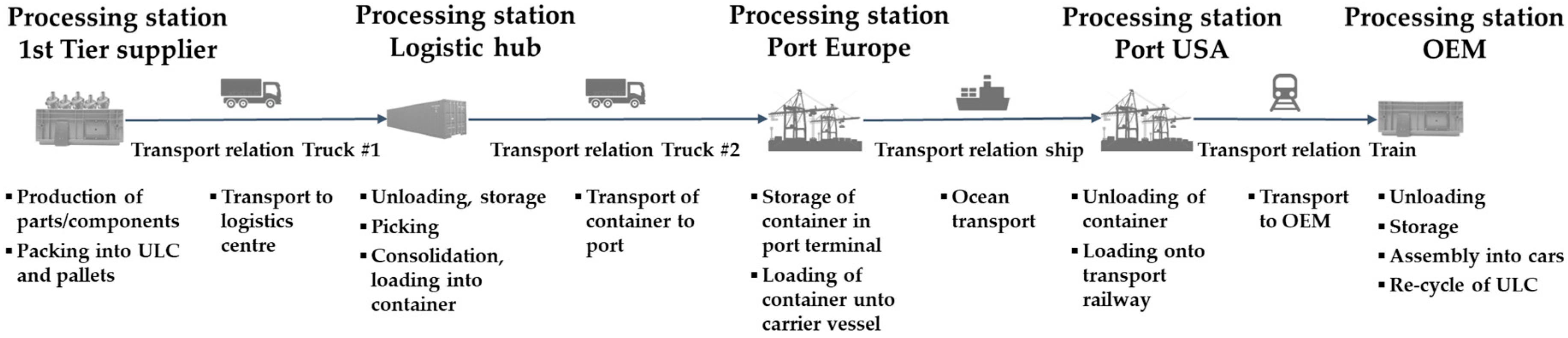
The model maps the supply chain process between a first tier supplier of automotive components located in Europe and an OEM, which receives these components in order to build them into its cars in a production plant located in Northern America. As shown in
Figure 1, they are connected by forwarders (shipping companies) using different transport modalities to transport the modules from the supplier to a logistics hub run by a logistics service provider (LSP), where the parts are consolidated into containers, and then further transported on ships across the Atlantic Ocean to the OEM.
The overall control of the supply chain is in the hands of the OEM. The supplier, LSP, and transporters all act on order of the OEM. Production of components at the supplier is triggered by a call order (make and take order) by the OEM for the production lot. These orders arrive in regular sequence, in order to maintain a steady supply for uninterrupted production. In addition, irregular call orders may be placed by the OEM in order to substitute for defective, or otherwise unusable, components. The readymade components are sent to a logistic hub by truck. At the logistic hub, an external logistic services provider (LSP) collects incoming components supplied to the same OEM by different suppliers and consolidates them into containers. However, the simulation model considers only one type of component. The LSP is also responsible for the timely, truck-based transport of the filled containers to a nearby container port terminal to reach a container vessel previously booked by the OEM.
At the container port terminal, the containers are loaded onto the container vessel. The vessel brings the containers to the destination port, where they are unloaded from the vessel and forwarded by train to the OEM’s production plant. At the plant, the parts are unloaded from the containers, and, after intermediate storage, built into the cars that are produced there. These processes are performed in the same way for regular orders by the OEM as well as for re-orders of components that cannot be used due to quality defects. The smallest lot size both for production and for transport is the universal load carrier (ULC), a standard box filled with 24 components.
Table 3 provides the details of the transport relations, including transport times, frequencies and volumes. The cargo volumes per transport of the different transport relations are synchronized with each other in order to achieve a steady situation.
The simulation model considers a carrier as smallest unit as the sensor decisions about the quality only happen per carrier. Each of the carriers contains 24 batteries, which are not modelled individually in the simulation model. A container contains 48 ULC, each filled with 24 components, and thus a container contains 1152 components. Every 75 s a battery is installed in a car, so every 30 min a ULC with 24 batteries is needed from the storage.
4.2. Scenarios
The simulation model contains four different scenarios in order to compare the effects of a sensor-based real-time quality information system on the control and operation of the modelled supply chain. These four scenarios differ in whether quality defects occur, and what quality management procedures are implemented.
Scenario 1 serves as a reference scenario in order to model the ideal state of the supply chain and evaluate different mechanisms without the occurrence of any quality defects. The reference scenario allows to determine component stock levels at the OEM that guarantee production not interrupted by stock-outs. Scenarios 2, 3, and 4 include quality defects occurring stochastically during the different transports. To detect quality defects, the simulation study considers two different quality management procedures: manual quality inspections (of random samples of the components) at the OEM’s warehouse entry (scenario 2) and sensor-based monitoring of environmental influences during the transport processes (scenario 3 and scenario 4).
The characteristics of the automotive components in the scenarios are derived from automotive batteries. Automotive batteries are sensitive products requiring careful treatment in logistic processes [
40]. For that reason, managing the quality of the batteries during transport is important. The simulation model accounts for such quality issues via stochastically distributed defect probabilities for each ULC filled with components and each transport relation. It is assumed that both the supplier and the LSP always inspect the quality of the outgoing, ready-made components at their warehouse exits, so that only defect-free components of good quality can leave. Subsequently, the model considers that with a certain probability, during each transport between the LSP and the OEM, components may become defective by suffering damage from environmental influences like heat, shock or humidity. For each transport relation between LSP and OEM, a defect probability is built into the model, which combines the probabilities of product damage from these environmental influences. This probability is the probability that a component will suffer damage during a transport using this transport relation. If no defects occur, the parts are of good quality. The defect and no defects probabilities for the transport relations are provided in
Table 4.
To cope with this risk of product defects, the simulation model includes the mapping of both conventional quality management procedures (without a sensor-based information system) and digital quality management procedures that are based on sensor measurements, as well as combinations of the two. In either case, safety stocks of the components at the OEM’s warehouse are the means to prevent the interruption of production at the OEM due to stock-outs that result from non-usable, defect components.
In this context, scenario 2 serves as a worst case scenario. It includes manual quality inspections at the OEM’s warehouse entry where quality defects of components are detected. However, this results in a late re-order of these components from the supplier.
Scenario 3 and scenario 4 both include sensor-based monitoring of environmental influences during transport. In contrast to these manual quality inspections at discrete points within the supply chain, the use of a sensor-based information system can generate quality-related data in real-time and thus support continuous product quality monitoring during the transport of the components.
In both scenarios 3 and 4, sensors are attached to the universal load carriers (ULC) accompany the components during transport, measure environmental influence parameters, like temperature, air humidity, and shock and send the measured data to a central, cloud-based quality information system. The sensor measurements are categorized according to a simple evaluation model that is based on information from the respective product data sheet. Based on this evaluation model the sensor measurements may be rated as “in order” (“OK”), “not in order” (“NOK”), or “undetermined”. The sensor measurements “undetermined” hints to environmental influences on a transport that may occasionally (more or less frequently), but not always, result in quality defects of the transported components.
Table 5 summarizes the probabilities for these sensor measurements in scenario 3 and scenario 4. In every transport relation, there is a certain number of transmission points. When a transport means (truck, ship, train) passes such a point, a sensor measurement is transferred. The number of transmission points in each transport relation is provided in the last line of
Table 5.
The model assumes that the sensors do not provide erroneous “OK” and “NOK” measurements. This means that “OK” sensor measurements only occur when the components are without defects and that “NOK” measurements only occur when components do indeed have defects. All the components without defects result in either “OK” or “undetermined” measurements. All defect components result in either “NOK” or “undetermined” measurements.
Of the undetermined measurements, the model assumes that 50% of them are prove defective at the OEM’s warehouse entry quality check, while the other half prove to be of acceptable quality for building into the cars, and that this is known to the sensor system provider.
Figure 2 shows the basic principle of the sensor-based quality control monitoring and corrective methods for scenario 3 and scenario 4. In both, scenario 3 and scenario 4, OK and to NOK measurements trigger the same reaction: If the sensor values are within their OK boundaries, no corrective measures are necessary. If measurements of a sensor that is attached to an ULC are rated as being not OK (NOK), because they exceed certain thresholds, the components in the ULC that the sensor accompanies are rated as “NOK”, and, as a corrective action, the same number of components is immediately re-ordered from the supplier to substitute for the NOK components.
The reaction to the third sensor measurement option “undetermined” is based on a combination of sensor-based quality monitoring and manual quality inspection at the OEM’s warehouse entry point. The reaction to this option differs between scenario 3 and scenario 4, as shown in
Figure 2:
In scenario 3, as shown in
Figure 2, part (a), the components accompanied by that sensor are be subject to a quality check at the arrival at the next supply chain node. This quality check results in the re-classification of the checked parts as “without defects” or “defect”. In the latter case, a re-ordering of the components to substitute for the NOK components is triggered.
In scenario 4, as shown in
Figure 2, part (b), sensor measurements of the category “undetermined” also result in the components accompanied by that sensor may be subject to a quality check at the arrival at the next supply chain node. However, parts are to be immediately re-ordered after the sensor measurement. As it is known that, on average, in 50% of the undetermined sensor measurement ratings the components accompanied by the measuring sensor are defect, this immediate re-order is carried out for every second ULC. For that reason, no parts have to be re-ordered at the manual quality inspection.
Table 6 summarizes the configuration of the four scenarios concerning the occurrence of quality defects of the components, the execution of a manual quality inspection at the OEM’s warehouse entry, the use of sensors monitoring environmental conditions in the transport chain, and the re-order policies for defect parts.
4.3. Simulation Experiments and Results
For each scenario, ten simulation experiments have been performed, each with a simulated time of 500 days. The simulation experiments compare the effects of the different quality management procedures that were implemented in the different scenarios. The parameter used for comparison is the difference (variation) between inventory levels at the OEM’s warehouse.
Figure 3 shows a screenshot of the simulation model in Tecnomatix PlantSimulation 14.1.
The inventory level at the OEM’s warehouse (inv
ULC, OEM) for a given simulated time t is calculated as the sum of the basic inventory, with which the simulation model is initialized at the beginning, and the cumulated components that have been re-supplied both on regular orders (r
ULC, reg, OEM), as well as on re-orders of quality defect components (r
ULC, qd, OEM) and that have already reached the OEM’s warehouse, less the cumulated ULC with defect components (d
ULC) that have been discharged so far (Equation (1)):
The days inventory held show for how many days a production with the currently stored amount of components (without any new components arriving) is possible. To calculate the days inventory held, the current inventory is divided by the necessary parts per day. In case of this simulation experiment, 48 carriers (each filled with 24 components) are needed per day (Equation (2)):
Table 7 lists the formula symbols used in Equations (1) and (2) and the units:
In each simulation experiment, the initial inventory level at the OEM’s warehouse is arbitrarily set at 2000 ULC (which equals 48,000 components). It takes roughly 20 days for the first ordered and produced components to arrive at the OEM. During that period, stored components are taken from the warehouse in order to build them into the cars at the OEM. After that initial period, components that are produced by the supplier start to arrive on a regular basis. Gradually, a stationary situation is reached, where average demand and production of components are on similar levels. The initialization phase of 50 days is not considered. For each of the three scenarios, the results of the ten simulation experiments have been averaged to determine the parameters for that scenario.
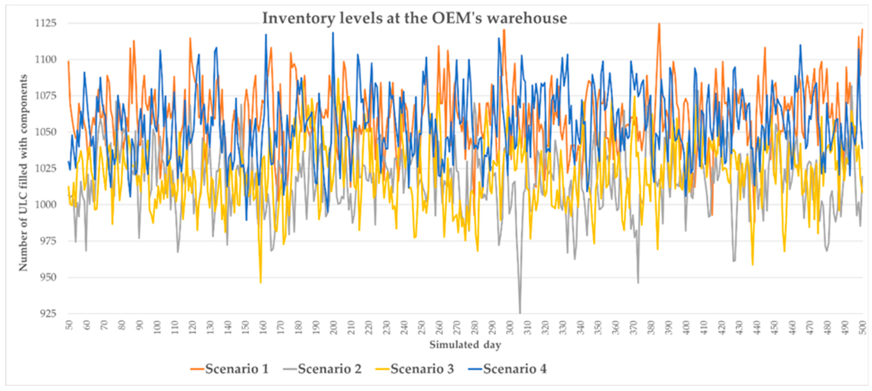
Figure 4 compares the development over simulated time of the components’ inventory levels at the OEM’s warehouse for scenarios 1, 2, 3, and 4:
They key parameters of inventory levels in each scenario are listed in
Table 8. The inventory levels differ in each scenario. In scenario 1, the OEM’s warehouse inventory levels are generally the highest, whereas, in scenario 2, they are generally the lowest. In scenario 3, they are higher than in scenario 2, whereas in scenario 4, they are almost as high as in scenario 1.
Table 8 also compares the spread of OEM’s warehouse inventory levels in each scenario by the difference between minimum and maximum inventory levels.
This difference between minimum and maximum inventory levels is the largest in scenario 2. In both scenario 3 and scenario 4, this difference is considerably smaller than in scenario 2. As the difference between minimum and maximum inventory levels determines the necessary safety stocks in order to prevent stock-outs of components, it can be concluded that, in scenario 3 and scenario 4, the safety stocks can be kept at a considerably lower level, as compared to scenarios 2.
5. Discussion
Mobile sensors can accompany, or be attached to, transported goods during transport processes and measure parameters like e.g., temperature or vibrations. These sensing devices generate an enormous volume of raw sensor data. In particular, raw sensor data tends to be very low-level and it must be further processed, analyzed, and transformed into higher-level information in order to be meaningful to applications and users. In the context of SCEM systems, critical quality related events have to be detected from the raw sensor data. These are events that indicate the occurrence, or increased risk of occurrence, of a quality defect, so that the quality of an article or component no longer conforms to the requirements or performs its function according to the specification.
Our conclusion from our examination of the relations between environmental influences and quality defects of automotive products is that actually determining changes in product quality from sensor data is not a trivial task. We have established that, during transport processes in supply chains, environmental influences may cause quality defects via failure mechanisms. These environmental conditions express themselves in, and can be derived from, physical or mechanical parameters, which in turn can be measured by mobile sensors attached to products/materials. For that reason, such mobile sensors, or networks of mobile sensors, attached to products allow for the monitoring of these environmental conditions and environmental influences affecting goods during transport processes by measuring environmental influence parameters, like e.g., temperature, air humidity, or shock, during transport processes. For that reason, sensors can detect critical, quality related events. Sensor measurements indicating certain physical parameters result in the information that certain environmental conditions are likely to cause quality damage.
However, it is difficult to determine critical events that have an impact on product quality during transport from sensor data, because it is difficult to determine which sensor measurements actually indicate conditions that are causing damage to products or deteriorate their quality.
The relations between environmental conditions and changes in product quality have to be captured in product related quality models, which are very specific to the individual characteristics of a product. Two methods are possible in order to establish a quality model:
Data Mining, Predictive Analytics, and Machine Learning methods: Data mining is the process of discovering patterns in large data sets involving methods at the intersection of machine learning, statistics, and database systems. It is used to extract information from a data set and transform the information into a comprehensible structure for further use. Predictive analytics encompasses a variety of statistical techniques from data mining, predictive modelling, and machine learning, to analyze current and historical facts to make predictions about future or otherwise unknown events. Machine learning is a subset of artificial intelligence in the field of computer science. Its task is to create and subsequently improve models that are based on the processing of training data. These models can predict new situations. Examples are artificial neural networks, support vector machines, and Bayesian networks [
41,
42].
Experimental determination of product specific susceptibility to failure mechanisms can use either destructive or non-destructive testing methods [
43]. In destructive testing, tests are carried out to the test object’s failure, in order to understand the test object’s performance or material behavior under different loads. Examples of destructive testing are stress tests, crash tests, hardness tests, and metallographic tests. Non-destructive testing (NDT) includes a large variety of analysis techniques to examine, inspect, and evaluate the properties of a material, component, or system without causing damage. It uses physical effects like electromagnetic radiation, sound and other signal conversions to examine metallic and non-metallic materials for integrity, composition, or condition with no alteration of the article undergoing examination. Methods include e.g., visual inspection, volumetric inspection with penetrating radiation, such as X-rays, neutrons or gamma radiation, or ultrasonic testing with sound waves, or the application of fine iron particles onto magnetized ferrous materials.
Data mining, predictive analytics, and machine learning methods are a proven instrument that can establish which sensor data indicate critical events with an impact on product quality. However, they need a large amount of real-life sensor data as well as detailed and reliable additional data on product quality and its changes, deteriorations and product damages in order to extract meaningful correlations. Experimentally derived product quality models also need a large amount of data. Non-destructive testing methods require an often-expensive infrastructure.
Destructive tests are generally easier to carry out, yield more information, and are easier to interpret than non-destructive testing methods. However, destructive testing methods consume several sacrificial products during the tests, thus increasing the costs. For this reason, destructive testing methods are suitable, and economic, for mass-produced objects.
As we have shown, product data sheets constitute an excellent source for the derivation of thresholds for sensor values in the absence of such quality models for individual products.
Our conclusion from the simulation study is that a sensor-based SCEM system that can consider quality aspects in real time can reduce costs and/or improve the logistic performance in an automotive supply chain.
A study of the 100 largest international automotive suppliers by McKinsey & Company, Düsseldorf, Germany, in cooperation with the European automotive supplier association CLEPA 100 predicts that digitalization of production in the context of Industry 4.0 has the potential to reduce quality related costs by 20%, e.g., by reducing product defects through data based real-time monitoring of production and logistics systems [
44].
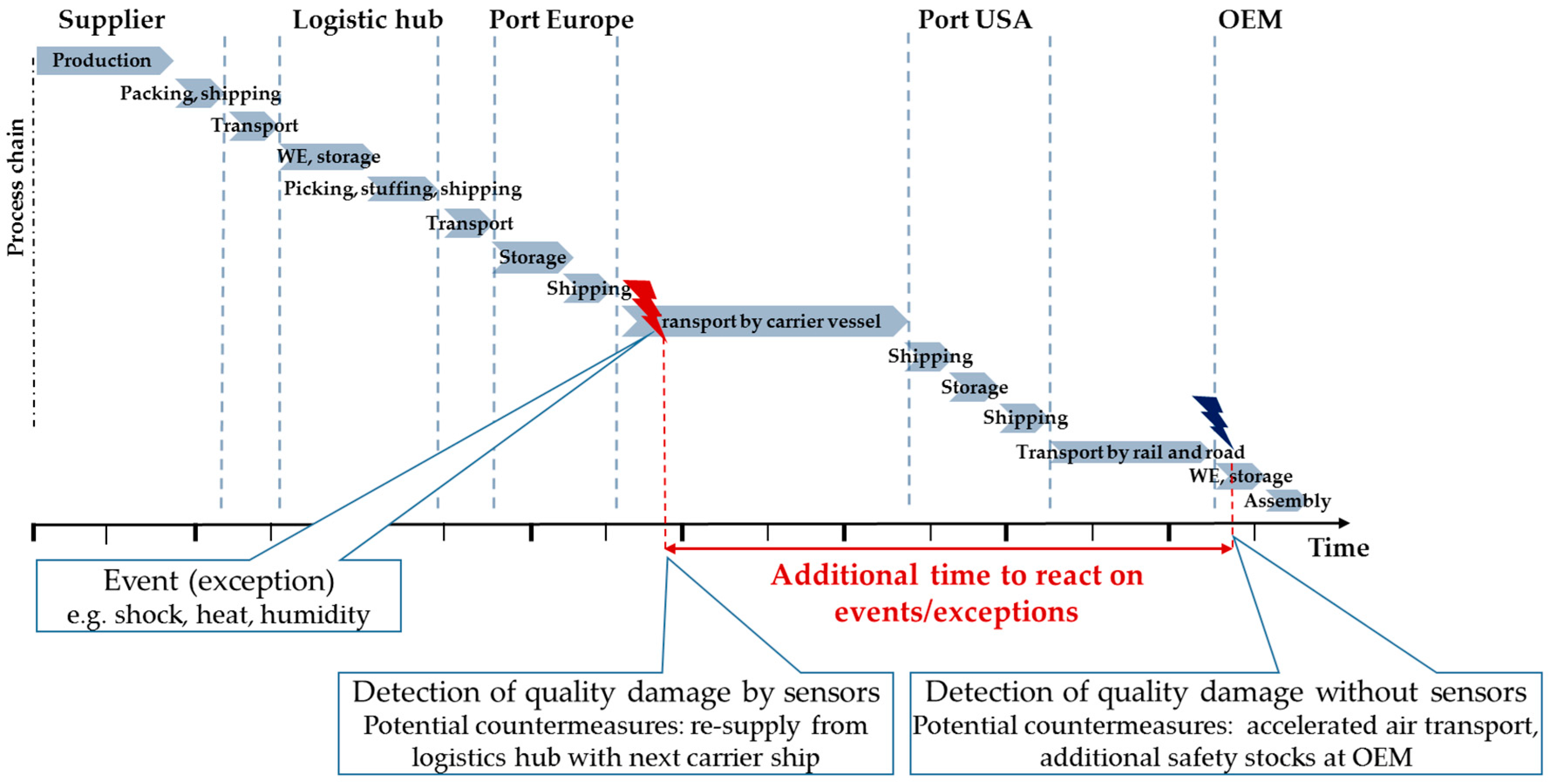
Our simulation study hints to that a sensor-based transport monitoring system can also reduce logistics related costs. In the simulation study, the scenario including a sensor-based monitoring system resulted in the lower safety stock levels needed to prevent production stock-outs. The stock levels can be even lower when parts are immediately re-ordered after suspicious sensor measurements, even if these do not necessarily indicate real defects. The main reason for this is the earlier recognition of quality problems and the longer reaction time (cf.
Figure 5).
Whereas, in a scenario with conventional quality management procedures, many quality defects that are caused by environmental influences during transport will only be recognized for the first time at the OEM’s warehouse entry, sensors accompanying the components during transport can send a message shortly after the event. For the supply chain that was examined in the simulation study, the time saving may amount to as much as two weeks in the case of a quality damaging event during sea transport. This allows for much earlier re-ordering of components, and consequently the timelier arrival of the re-ordered components at the customer.
6. Conclusions
This paper has described an approach for monitoring transport processes in automotive supply chains using sensor data. Mobile sensors accompanying transport goods combined with telematics and digital services can continually provide data on environmental influences affecting these goods via failure mechanisms. The influences of environmental conditions on automotive components and products depend foremost on the materials used.
Our simulation has shown how use of sensor data in an event-driven control of material flows can reduce the necessary safety stock levels of components in an automotive supply chain.
In conclusion, planning and control of networked production and logistics processes in the automotive industry can be improved by the timely consideration of sensor-based quality data. Individual product quality models are needed to describe the effects of environmental influences on failure mechanisms for individual products in the necessary detail that is required to translate sensor measurements into product quality relevant data.


