Design of Delivery Valve for Hydraulic Pumps

Abstract

After briefly recalling the main problems that arise in the study of globe valves for alternative pumps, a methodology has been set up in order to refine the design. The obtained method has the advantages of simplicity and independence from empirical diagrams. In summary, from the obtained equation, the suitable values of the parameters can be deduced, based on the assigned data (capacity Q₀ and number of rounds n) of all the dimensions of the valve or of the valves. Depending on the parameter values, it is possible to identify the most suitable kind of valve: a single dish-shaped valve, a ring valve, a valve with several rings or a group of valves.

1. Introduction

Automatic valves for suction and delivery are the most important components of a piston pump, since the wear and locking of a valve, in addition to greatly reducing capacity, can also cause serious deformations of the piston rod. Therefore, it is necessary to design such mechanical components with care and with the use of high-quality materials [1,2,3,4].

Regarding the type of valve which should be used, it is possible to provide only indicative data: valves with a conical seat, having no return springs, are suitable for low flow and low speeds. By increasing the capacity, valves with multiple seats must be used, and for high rotating speeds, it will be necessary to use return springs, which allow a more rapid closure, improving volumetric efficiency. To prevent the leakage of the liquid through the passage hole for the rod of the plunger, stuffing boxes with flexible seals are generally used, fixed at the end part of the cylinder or added there with a series of bolts [5,6,7,8,9,10].

In the annular cavity surrounding the rod, rings of hemp or asbestos graphite are inserted, which are then compressed by the mobile collar, properly tightening the bolts that attach it to cylinder. The rings adhere more or less strongly to the piston rod, limiting fluid outflow; the adjustment of the bolts must be very accurate because over-tightening may cause the heating of the rod and of the packing gland, while tightening too weakly can cause a substantial loss of liquid and thus a decrease of the volumetric efficiency [11,12,13,14,15,16].

A complete methodology for the sizing of the control valve passes through the definition of its size and its degree of opening during the design capacity. As a first approach to a “default”, it is necessary to choose a size of valve with a nominal diameter minutely smaller than the diameter of the line. In any condition, it is possible to use a “line size” valve. This choice identifies the capacity coefficient (commonly known as CV) of the valve. The CV full opening of a control valve is the number of US gallons/minute that flow through the considered valve with a pressure drop of 1 psi. The load losses in the valve are regulated by the degree of opening that the valve has in its design capacity. The opening fraction (expressed in formulas) is the ratio of the actual CV and full opening CV. Normally, this value is chosen (computed with design capacity) between 60% and 90% [17].

In the study of the motion of a piston pump valve [18,19,20,21,22,23], it is necessary to take into account three speeds:

-

the v of the fluid, which depends on the load loss corresponding to the passage through the valve;

-

v′, which affects the water pressure acting against the dish-shaped valve;

-

and the v_v of the dish-shaped valve of the considered system.

Further, it is necessary to consider also the diagrams of the valve lift depending on the crank and the piston position; in a first approximation, these diagrams can be reduced to very simple schemes.

Finally, it is interesting to show that the maximum valve opening depends on the pump capacity but not on individual factors (run, area of the piston and number of the round of the crank), singly considered, that determine the pump capacity.

Of all these issues, very little is reported in the current literature. Therefore, in this study, we will proceed by beginning to establish, in an approximate way, the relationships between the main variables that influence the considered phenomenon.

Subsequently, corrections have been performed, aimed at determining the best operating conditions of the valves considered.

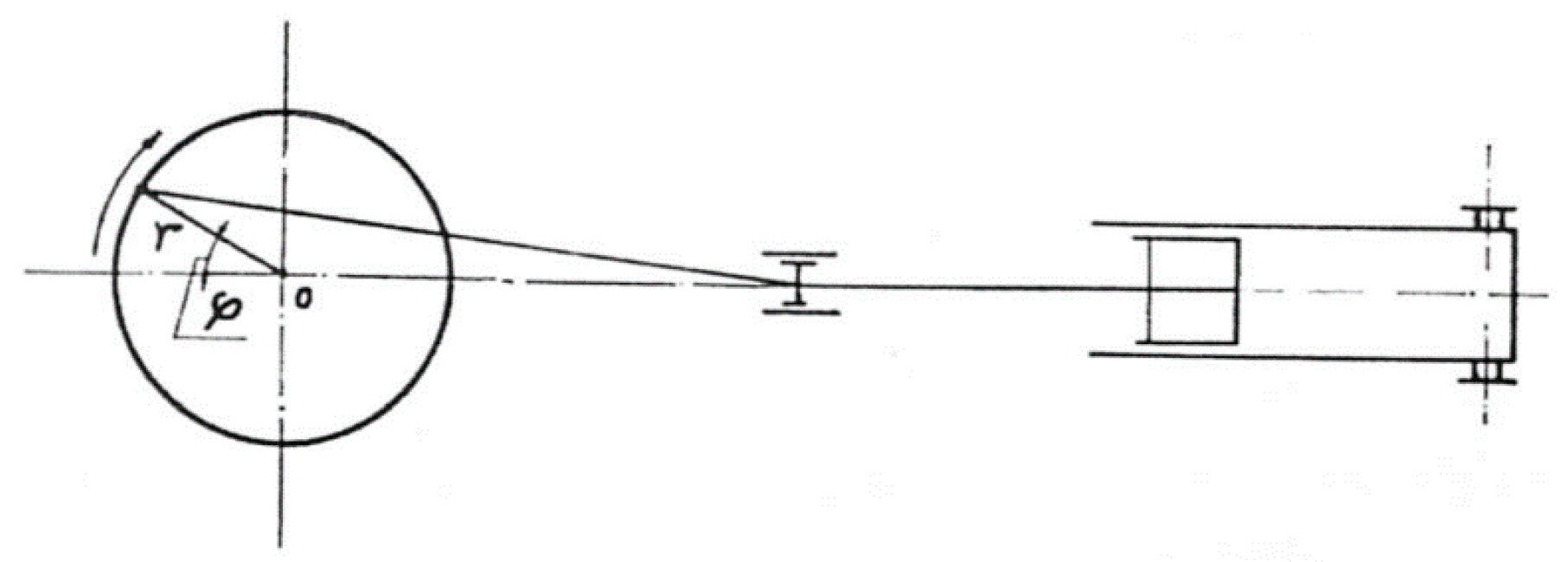
2. Preliminary Analysis

Before getting started, an approximate analysis has been performed, and corrections have been added afterwards in order to lead to a precise representation of the considered phenomena.

As an example, we can consider the pump in the delivery phase (Figure 1) with $\omega$ = const. If the obliquity of the connecting rod is neglected, the stroke s of the piston is given by

$$s=-r·\cos \overline{\omega }·t$$

(1)

Knowing that u = $\omega r$, the velocity of the piston can be written as follows

$$v_s=u·\sin \overline{\omega }·t.$$

(2)

Furthermore, naming F as the piston surface, the instantaneous capacity, Q, will be

$$Q=Fu\sin \phi$$

(3)

If h is the height at the instant t, $\delta$ the angle of the seat and l the peripheral development of the hole (Figure 2), the cross-section f of the latter will be, at the instant t,

$$f=l·h·\sin \delta$$

(4)

Then, if v is the theoretical speed of the water through the hole and $\mu$ the flow coefficient, this will result in the following:

$$Q=f·\mu ·v$$

(5)

From (3) and (5), we immediately obtain

$$F·u·\sin \varphi =f·\mu ·v$$

(6)

and for (4)

$$h=\frac{F·u·\sin \varphi }{\mu ·v·l·\sin \delta }$$

(7)

If now it is assumed in first approximation that $\mu ·v$ is constant, this will also be true for the coefficient of $\sin \varphi$ at the second member of (7), a coefficient which gives the maximum height h_max occurring for $\phi$ = $\pi$/2; then, (7) can be written

$$h=h_{\max }·\sin \phi$$

(8)

Using Formula (8), reporting the angles $\phi$ on the x-axis and the height h on the y-axis, we obtain a sinusoid with amplitude h_max. From (1), it is possible to obtain

$$\frac{s}{r}=-\cos \varphi$$

While from (8) we obtain

$$\frac{h}{h_{\max }}=\sin \varphi$$

Thus, by squaring and summing we will obtain the relationship:

$$\frac{s^2}{r^2}+\frac{h^2}{h_{\max }^2}=1$$

In addition, reporting the distances travelled by the piston starting from the midpoint of its curve on the x-axis and the risers of the valve on the y-axis, we obtain an ellipse, with axes r and h_max.

It is clearly possible to see that, in this first approximation, the valve should open and close precisely in the instants in which the piston is located at the dead points. Now, it is possible to show easily the expression of the section f_max of the valve’s maximum opening. In fact, from (6) we obtain

$$f=\frac{F·u·\sin \varphi }{\mu ·v}$$

(9)

and

$$u=\omega ·r=\frac{\pi ·n·r}{30}$$

(10)

will be

$$f=\frac{\pi ·F·n·r\sin \varphi }{30·\mu ·v}$$

(11)

but

$$\frac{F·n·r}{30}=Q_0,\left(Q_0=const.\right)$$

(12)

and then

$$f=\frac{\pi ·Q_0}{\mu ·v}\sin \varphi$$

(13)

from which

$$f_{\max }=\frac{\pi ·Q_0}{\mu ·v}$$

(14)

Thus, for the supposed constancy of $\mu ·v$, it is possible to demonstrate the assumption that f_max (and therefore h_max, with parity of l) depends on the product valve $F·n·r$ (=30 Q₀) and not from each of the factors considered, F, r, n. Now,

$$P=T+G·\left(1-\frac{{\gamma }_1}{\gamma }\right)$$

(15)

where T is the spring load on the dish-shaped valve, G is the weight of the valve, ${\gamma }_1$ is the specific weight of the pumped liquid and $\gamma$ is that of the material of which the valve is made. The product G (1 − (${\gamma }_1/\gamma$)) is the reduced weight of the valve from the hydrostatic thrust (we suppose the valve moving vertically) and P, in absolute value, is the thrust of the water on the considered valve. Since T is a function of h, the same thing will happen for P, with f₁ indicating the area of the section of the valve in the plane of the seat, approximately equal to the surface of the valve, which is

$$b=10\frac{P}{f_1}$$

(16)

The ratio (P/f₁) is expressed in atmospheres. Formula (16) gives the pressure in N/m².

Pressure b corresponds, in known different conditions, to the theoretical speed of outflow:

$$v^{\prime }=\sqrt{2·g·b}$$

for which the actual value through the valve hole can be put,

$${\mu }_p·v^{\prime }={\mu }_p·\sqrt{2·g·b}$$

(17)

indicating ${\mu }_p$, a particular flow coefficient determined experimentally and which depends on the type of valve considered. Then,

$$Q=f·{\mu }_p·\sqrt{2·g·b}$$

(18)

in comparison with (5) gives

$$\mu ·v={\mu }_p·v^{\prime }={\mu }_p\sqrt{2·g·b}$$

(19)

The hypothesis of the $\mu v$ constant implies therefore that ${\mu }_p·v^{\prime }$ is constant. On the other hand, with f being the area of the outflow aperture hole, the following must be true:

$${\mu }_p·\sqrt{2·g·b}=\mathit{const}.$$

(20)

with f and Q variables, however, for μv′ constant must be Q/f constant Assumed known μ_p from (18) we obtain

$$b=\frac{Q^2}{2{g·f}^2{\mu }_p^2}$$

(21)

which allows us to deduce b, if Q is known. To keep Q constant, the product must obviously be $b{\mu }_p^2$. Then, the velocity v_v of the valve, is obtained from (8):

$$v_v=\frac{\mathit{dh}}{\mathit{dt}}=h_{\max }·\cos \varphi$$

(22)

which explains that the speed of the valve reported on the ordinate in the function of the time (or of the angles $\varphi$) gives rise to a cosinusoid. Formula (22) also indicates that, for $\varphi =$0 and for $\varphi =\pi$, v_v ≠ 0, so that the valve opens and closes with finite speed; i.e., with shock.

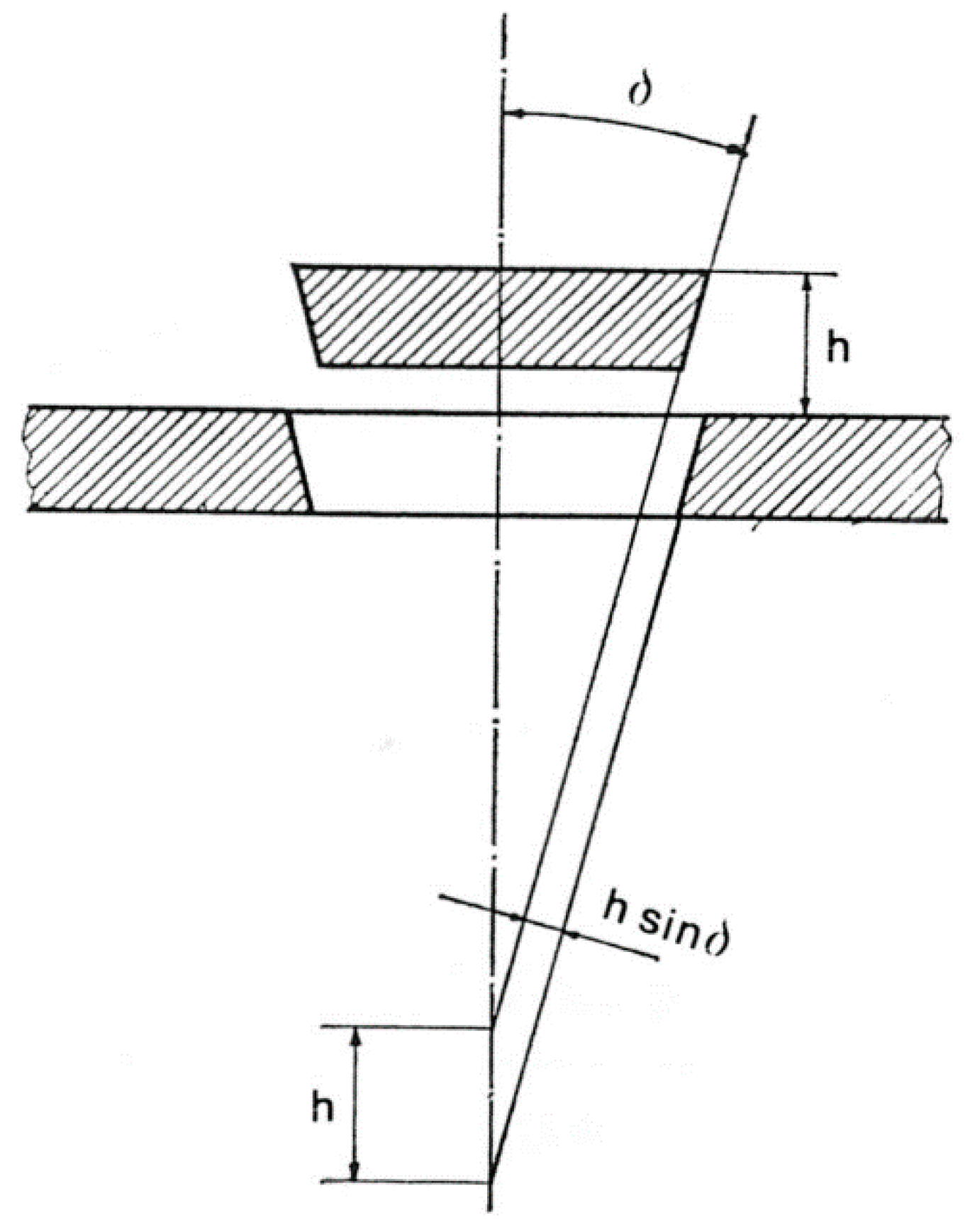
3. Additional Effects and Their Influence

Establishing the basic relationships on the motion of the valve and the water through it, on the basis of this simple hypothesis, it is possible to perform a closer examination by introducing some important corrections such as the piston effect of the valve, the variability of the product $\mu v$, the obliquity of the connecting rod, etc.

As regards the plunger effect of the valve, we examine v_s, and v_v in the function of $\varphi$, supplied respectively by (2) and (22).

For $\varphi$ < $\pi$/2, in the infinitesimal time dt, the plunger will tend to push the volume Fv_s dt over the valve. Then, the valve, in the phase of turning away from the seat, will generate, upstream of the outflow aperture hole, the volume f₁ v_v dt, so that not all of the water pushed by the piston is able to pass through the free hole.

Conversely, per $\varphi >\pi /2$, the valve will be coming closer to the seat and it forces to go through the clearance hole, not only the volume Fv_s dt driven by the piston, but also the f₁ v_s dt pushed by it.

Since these volumes, for the constancy of F and f₁, are proportional to v_s and v_v, it is easy to obtain the values of the instantaneous flows that pass downstream of the delivery valve. From these results, the simplifying assumptions made about the motion of the valve lead us to admit that for very small $\varphi$, the valve is in an opening phase while the liquid passes from downstream to upstream of it, which is impossible, because of the occurrence of a pressure that forces the valve to move in the opening direction.

Therefore, the delivery valve remains closed until $\varphi$ not has reached a certain value, which is also rather small. Further, the delivery valve cannot take place for exactly $\varphi =\pi$, but must occur with a determined delay. Therefore, we have to evaluate this delay, and hence the speed with which the collision takes place, during the closure of the delivery valve. Then, we compute the volume that passes through the free span in the time unit with the difference between the volumes generated by the piston and by the valve, and in such a condition, we determine the instantaneous valve lift. Therefore, we will have the relationship

$$f·\mu ·v=F·v_s-f_1·v_v$$

from which, substituting at f the value from (4), at v_s the value from (2) and at v_v the value from (22), we get

$$\mu ·v·l·h·\sin \delta =F·u·\sin \varphi -f_1-h_{\max }\overline{\omega }\cos \varphi$$

from which

$$h=\frac{F·u}{\mu ·v·l·\sin \delta }·\sin \varphi -h_{\max }\frac{f_1}{\mu ·v·l·\sin \delta }\omega \cos \varphi$$

Now, the coefficient of sinφ in the (7) is h_max so we can write the following:

$$h=h_{\max }\left(\sin \varphi -\frac{f_1}{\mu ·v·l·\sin \delta }·\omega \cos \varphi \right)$$

(23)

from which it is possible to obtain the angular delay $\psi$, as that value of $\varphi$ at which h = 0. This should, however, proceed as follows.

Deriving the (23) respect to time, it is possible to obtain a new expression, approximated in a better way, of the valve speed:

$$v_v^{\prime }=h_{\max }·\omega ·\left(\cos \phi +\frac{f_1}{\mu ·v·l·\sin \delta }·\omega ·\sin \phi \right)$$

from which we obtain the impact speed in the closure phase:

$$v_c=h_{\max }·\omega ·\left[\cos \left(\pi +\psi \right)+\frac{f_1}{\mu ·v·l·\sin \delta }·\omega ·\sin \left(\pi +\psi \right)\right]$$

(24)

Assuming that such a delay is small enough, $\sin \left(\pi +\psi \right)=$0 and $\cos \left(\pi +\psi \right)$ = −1 may be assumed; with that, (24) reduces to the simple relation

$$v_c=-\omega ·h_{\max }$$

(25)

which for (7), (8) and (19), becomes, with u = ω·r,

$$v_c=\frac{-F·{\omega }^2·r}{{\mu }_p{v}^{\prime }·l·\sin \delta }$$

(26)

The kinetic energy dissipated in the impact, named M the valve mass, it will then be for (26)

$$\frac{1}{2}M·v_c^2=\frac{1}{2}M{\left(\frac{F·{\omega }^2·r}{{\mu }_p·v^{\prime }·l·\sin \delta }\right)}^2$$

(27)

Referring this force at the section of the valve, with G being the weight of the valve, will get the additional relationship

$$\frac{1}{2}M·v_c^2={\xi }_1\frac{G}{2g·f_1}{\left(\frac{F·{\omega }^2·r}{{\mu }_p{v}^{\prime }·l·\sin \delta }\right)}^2$$

(28)

in which the correction factor ${\xi }_1$, takes into account the water dragged by the valve.

Placing (πn/30) for ω and taking account of (12) and (19) occurs after a few steps:

$$\frac{1}{2}\frac{M·v_c^2}{f_1}={\xi }_1\frac{G{\pi }^4}{4·g^2·f_1}{\left(\frac{Q_0·n}{30·{\mu }_p·\sqrt{b}·l·\sin \delta }\right)}^2$$

(29)

Now this specific force has not to exceed a determined value, so that the impact in the closure phase is not very violent, to put in a short time, out of the work the valve; on the other hand, it is necessary that the same living force is not too small, otherwise too large valve dimensions are obtained. It is therefore appropriate that it has an almost constant value. Welding together all of the numeric values in this constant, it is appropriate to set

$$C·\sin \delta =\frac{Q_0·n}{l}\sqrt{\frac{G}{b·f_1}}$$

(30)

with C·sinδ = 1.3 ÷ 1.9, as experience suggests conservatively.

In Formula (30), Q must be expressed in L/s, f₁ in cm², b in m of water column, and l in cm, and it is possible to note that, if a given valve has operated satisfactorily in a pump with flow Q₀ and number of rounds n, it will be able to work equally well in any other pump in which the product Q₀ n is the same value.

Meanwhile, from (6), we obtain

$$f=\frac{F·u·\sin \varphi }{\mu ·v}$$

and then

$$f_{\max }=\frac{F·u}{\mu ·v}$$

but u = (π·n·r)/30 and f_max = h_max·l·sinδ are then, on basis of (12),

$$h_{\max }=\frac{\pi }{l·\mu ·v·\sin \delta }·Q_0$$

Then, it is possible to set

$$n·h_{\max }=C·Q_0·n\left(\mathrm{with}C=const.\right)$$

(31)

and repeat for the value of the product n·h_max what was said for Q₀ n: the valve will work in the same way (equally good or bad) for the same value of the product n·h_max. However, because it is necessary that by varying h_max, Q₀ does not change, it is necessary to change h_max only within small limits that ensure that the load on the valve does not alter simultaneously.

While the (30) is useful for the completely new design of a valve (this case happens very rarely), the considerations relating to the products Q₀ n and n·h_max are extremely useful for the adaptation of valves already designed for load conditions which are rather different to those assigned.

4. Design Method

To design a valve, it is therefore necessary that, given the pump capacity Q₀, it is possible to obtain f_max from the relationship (14) after fixing a convenient value for μ·v based on the following data and criteria:

-Pumps for exhaustion (small prevalence)	μ·v = 1÷2 m/s
-Pumps for large prevalence	μ·v = 1.5 ÷ 2.5 m/s
-Pumps for draining mines	μ·v = 2 ÷ 3 m/s
-Pumps for high pressures	μ·v = 3 ÷ 5 m/s

observing that μ·v must be lower for small prevalences.

Obtaining the f_max value, it is necessary to split this value into the two factors h_max and l, setting preferably h_max so that it is still possible to perform when the type of valve is simply chosen based on available data related to valves already built of the same type. If these data are not available, it is possible to follow the following indications.

For φ = π/2, the valve has zero speed, as shown by (22); so, the piston effect being null, it is possible to use the formulas of the elementary theory first established with full accuracy, without the effect considered. Then, the variable light will actually be at its maximum aperture f_max (corresponding to the maximum value h_max of the lift), and only the water displaced by the piston will pass through this.

For φ = π instead, the valve will still have a lift h₀ that can be calculated on the basis of the hypothesis of the constancy of the outflow speed μ·v since, stopping the piston, water will pass through the corresponding opening of the valve (pumped from the valve considered) providing the speed as reported in (22). The above-mentioned hypothesis allows us then to suppose that the risers h₀ and h_max are proportional, respectively, to the instantaneous flow f₁·v_vmax and f_max·v, and this therefore allows us to write, on the basis of (22),

$$\frac{h_0}{h_{\max }}=\frac{\frac{\pi ·n}{30}·f·h_{\max }}{f_{\max }·\mu ·v}$$

(32)

In the case, e.g., of a ring valve with a mean diameter d_m = (d_e + d_i)/2 and a radial width a = (d_e − d_i)/2, the following will be true:

$$f_1=\frac{\pi }{4}\left(d_e^2-d_i^2\right)=\pi ·a·d_m$$

(33)

On the other hand,

$$f_{\max }=2\pi ·d_m·h_{\max }·\sin \delta$$

(34)

from which (32) becomes

$$\frac{h_0}{h_{\max }}=\frac{\pi ·a·n}{60·\mu ·v·\sin \delta }$$

(35)

Now, experience has shown the following can be accepted from handbooks [24,25]:

$$\frac{h_0}{h_{\max }}=\frac{1}{20}÷\frac{1}{60}$$

(36)

Thus, (35) leads to the relationship

$$\frac{\pi ·a·n}{60·\mu ·v·\sin \delta }=\frac{1}{20}÷\frac{1}{60}$$

(37)

in which a is expressed in m, with v being expressed in m/s. Wanting to express a in cm, it is necessary to write

$$\frac{\pi ·a·n}{100·60·\mu ·v·\sin \delta }=\frac{1}{20}÷\frac{1}{60}$$

That is,

$$\frac{a}{\sin \delta }=\kappa \frac{\mu ·v}{n}$$

(38)

with k ranging between 30 and 100.

Assigning n, and μ·v being already fixed, as has been said discussing (14), Formula (38) allows us to establish a/sinδ so that, in the case of the ring valve, if it is accepted that the speed in the section (π/4) (d_e² − d_i²) = π·a·d_m is equal and that f_max = 2·π·d_m·h_max·sinδ (see (33) and (34)), its value is 2·h_max.

In fact, it has to be

$$Q_0=\mu ·v·\pi ·a·d_m=\mu ·v·2\pi ·d_m·h_{\max }·\sin \delta$$

and from the equality of the last members,

$$\frac{a}{\sin \delta }=2·h_{\max }$$

(39)

Replacing the precedent in (38), we have

$$\frac{2·h_{\max }·n}{\mu ·v}=\kappa$$

and then

$$h_{\max }=\kappa ·\frac{\mu ·v}{2·n}$$

(40)

As either a and d_m do not appear in (40), it is also true in the case of the valve that is possible to verify this by placing a = d_m = d/2 in the previous formulas.

It is necessary to show that the method shown has the merit of the simplicity and independence from empirical diagrams (such as those of μ_p, etc.), but it is not sure that the limits set for the $\kappa$ in (40) are valid in general for all types of valves.

Summarizing from (14) and (40), with v and k suitably chosen, on the basis of the data Q₀ and n, all the dimensions of the valve or of the valves can be deduced. Depending on whether l = (f_max)/(h_max sinδ) results in a small or large value, we will choose, in order, a single dish-shaped valve, a ring valve, a valve with several rings or a group of valves. This may require some testing, and it is clear that for the dish-shaped valve and for that with a single-ring, we obtain, respectively,

$$d=\frac{l}{\pi }\mathrm{and}{d}_m=\frac{l}{2·\pi }$$

(41)

In the case of the ring, the knowledge of d_m is not sufficient, but because it is necessary to know d_e and d_i, or a, it is possible to use the relationship between the value obtained in identifying the speed in the light constant with that in the light variable, namely supposing (39) is valid or assuming the a value to be somewhat larger, for reasons of working as well as to reduce friction losses.

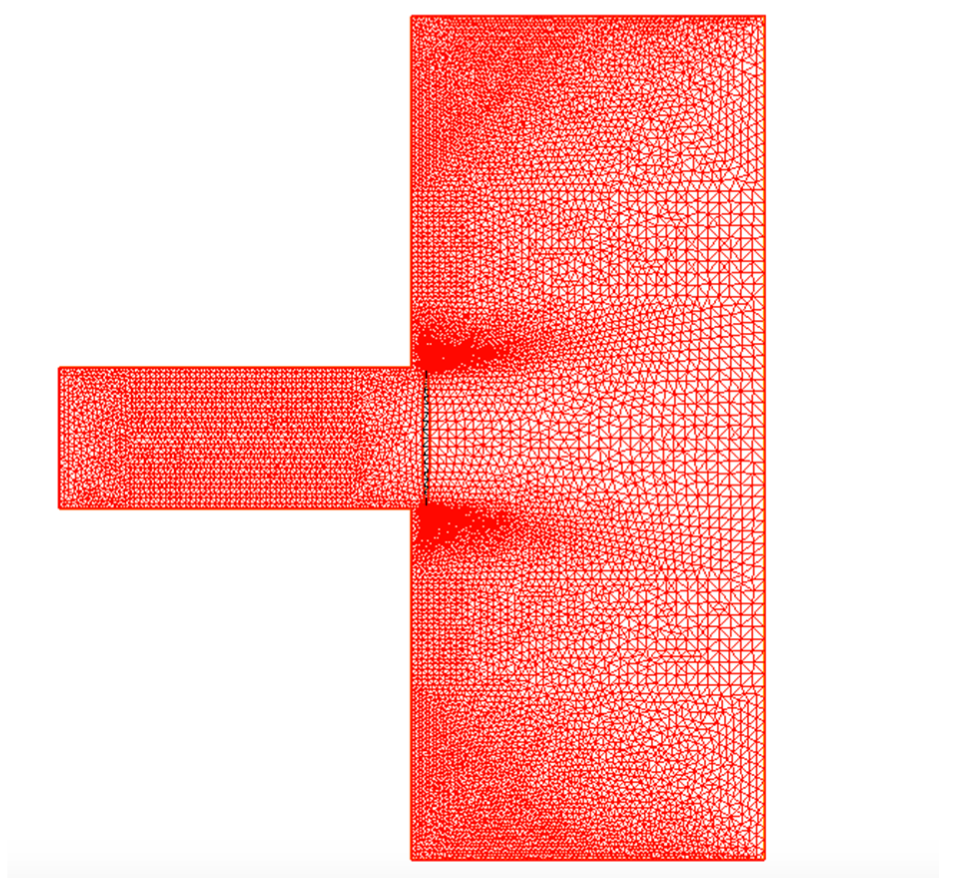
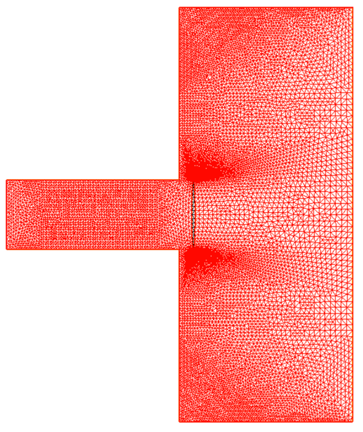
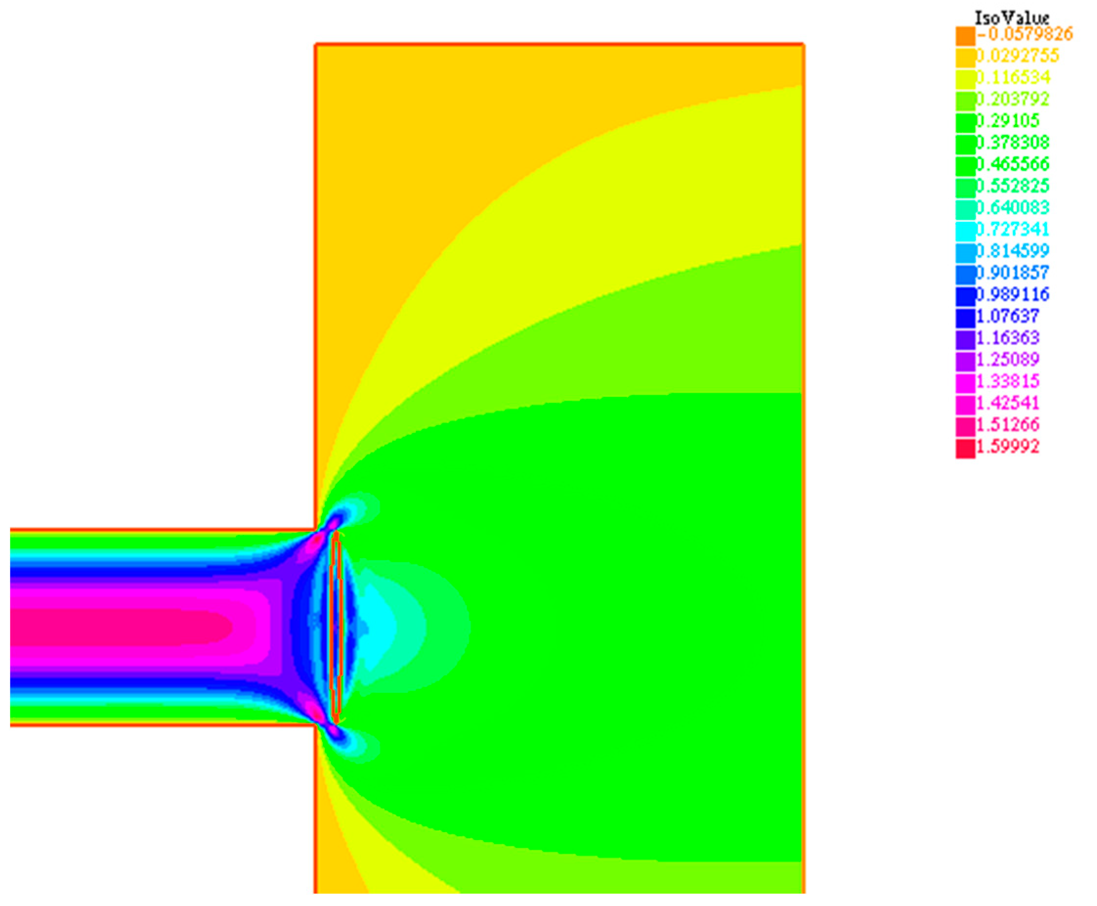
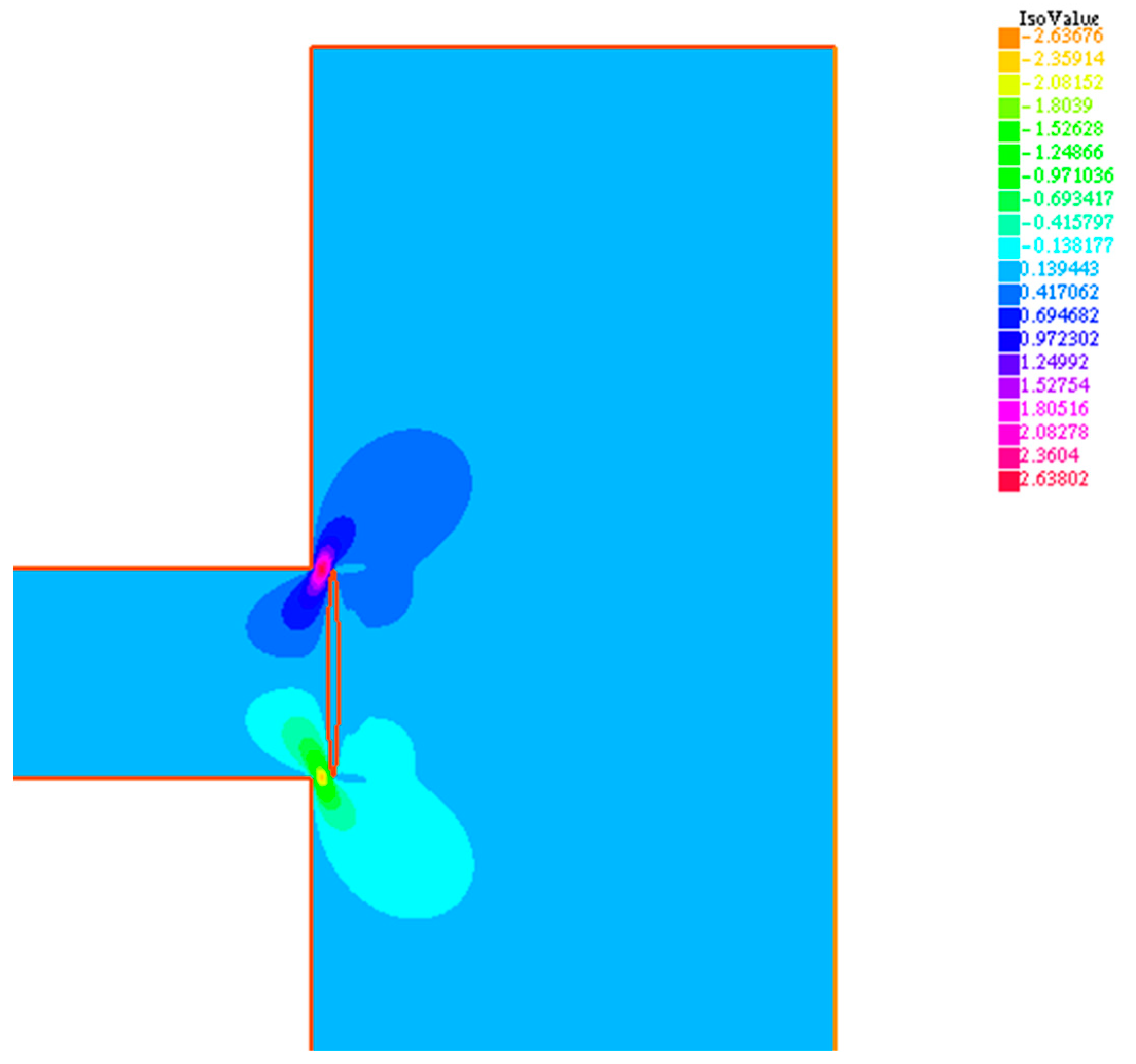
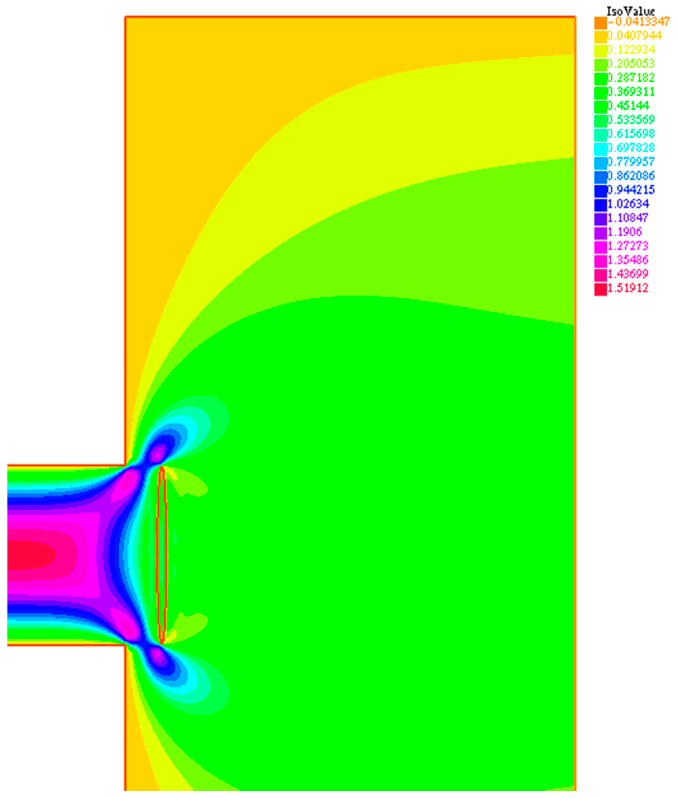
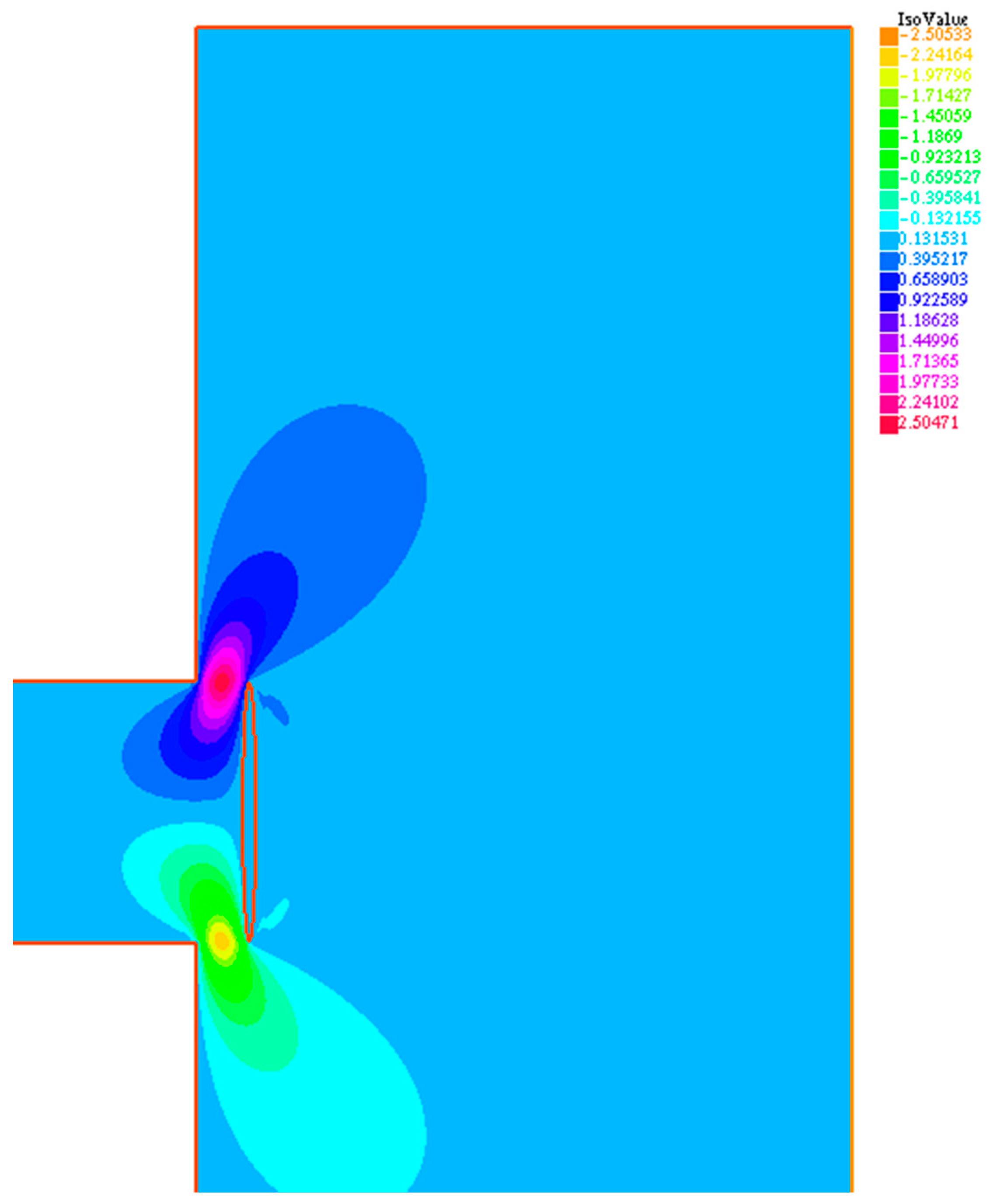
5. Numerical Simulation

To better understand the working of the considered dish-shaped valve, two numeric simulations were performed for the scheme reported in Figure 2, considering two operating conditions, relating to two positions of the dish-shaped valve: case 1, with a plate opened with only 3 mm of lift; case 2, with the plate open with 10 mm of lift, considering a pump working with water at the standard pressure.

Therefore, the flow inside a pipe was examined, partialized by a considered plate-shaped valve. All simulations were performed with the commercial code FLUENT. The time integration step has been chosen so as to ensure the fulfillment of the stability constraints of the numerical scheme used. These methods were applied also in other papers [26,27,28,29,30,31,32,33,34,35,36,37,38,39,40,41,42,43,44,45].

For this application, we chose a case where the Reynolds number was based on the pipe diameter, D, and the maximum speed u_max inside the pipe is 400. The simulation of the equations was carried out without the addition of filters or turbulence models. The resulting field, shown in the following figures, is, therefore, the result of a numerical integration of the Navier–Stokes equations. The numerical models’ mesh for the considered cases are reported in Figure 3 and Figure 4. In Figure 5 and Figure 6, characterized by a valve opening of 3 mm, the horizontal and vertical velocity components for case 1 are reported. It can be noted how the valve induces a substantial change of the flow within the pipe. This condition also corresponds to the greater loss of pressure of the flow and the maximum load condition among the considered configurations. In Figure 7 and Figure 8, characterized by an opening of the valve of 10 mm, the horizontal and vertical velocity components for case 2 are reported. In this condition, the flow lines show the spatial structure of the motion field inside the pipe.

6. Conclusions

In this paper, a methodology to refine the design of a delivery valve for hydraulic pumps has been set up to examine the problems that arise in the study of dish-shaped valves for alternative pumps. The obtained method has the advantage of ease of use and does not depend on empirical diagrams. On the basis of the different equations obtained, with the parameter values suitably chosen, it is possible to deduce, based on the data assigned (capacity Q₀ and number of rounds n), all the sizes of the considered valves. Depending on the considered parameter values, it is possible to choose, in order, a single dish-shaped valve, a ring valve, a valve with several rings or a group of valves.

Further, to better understand the working of the pump dish-shaped valve, two operative conditions have been considered, with valve openings of 3 mm and 10 mm, evaluating the motion field obtained.

References

1. Akers, A.; Gassman, M.; Smith, R. Hydraulic Power System Analysis; Taylor & Francis: New York, NY, USA, 2006. [Google Scholar]
2. Pappalardo, C.M.; Zhang, Z.; Shabana, A.A. Use of independent volume parameters in the development of new large displacement ANCF triangular plate/shell elements. Nonlinear Dyn. 2018, 91, 2171–2202. [Google Scholar] [CrossRef]
3. Cho, J.; Zhang, X.; Manring, N.D.; Nair, S.S. Dynamic Modelling and Parametric Studies of an Indexing Valve Plate Pump. Int. J. Fluid Power 2002, 3, 37–48. [Google Scholar] [CrossRef]
4. Barbagallo, R.; Sequenzia, G.; Cammarata, A.; Oliveri, S.M.; Fatuzzo, G. Redesign and Multibody Simulation of a Motorcycle Rear Suspension with Eccentric Mechanism. Int. J. Interact. Des. Manuf. 2017, 12, 517–524. [Google Scholar] [CrossRef]
5. Rivera, Z.B.; De Simone, M.C. Waypoint Navigation for Autonomous Mobile Robots in Ros-based Environments. Robotics 2018, submitted. [Google Scholar]
6. Rahmat, M.F.; Rozali, S.M. Modeling and Controller Design of an ElectroHydraulic Actuator System. Am. J. Appl. Sci. 2010, 7, 1100–1108. [Google Scholar] [CrossRef]
7. Pappalardo, C.M.; Wang, T.; Shabana, A.A. Development of ANCF tetrahedral finite elements for the nonlinear dynamics of flexible structures. Nonlinear Dyn. 2017, 89, 2905–2932. [Google Scholar] [CrossRef]
8. Loukianov, A.G.; Rivera, J.; Orlov, Y.V.; Teraoka, E.Y.M. Robust trajectory tracking for an electro-hydraulic actuator. IEEE Trans. Ind. Electron. 2009, 56, 3523–3531. [Google Scholar] [CrossRef]
9. De Simone, M.C.; Guida, D. Modal coupling in presence of dry friction. Machines 2018, 6, 8. [Google Scholar] [CrossRef]
10. De Simone, M.C.; Rivera, Z.B.; Guida, D. Finite element analysis on squeal-noise in railway applications. FME Trans. 2018, 46, 93–100. [Google Scholar] [CrossRef] [Green Version]
11. Battistoni, M.; Foschini, L.; Postrioti, L.; Cristiani, M. Development of an Electro-Hydraulic Camless WA System. SAE Tech. Pap. 2007. [Google Scholar] [CrossRef]
12. Turner, C.; Babbitt, G.; Balton, C.; Raimao, M. Design and Control of a Two-stage Electro-hydraulic Valve Actuation System. SAE Tech. Pap. 2004, 1, 1265. [Google Scholar]
13. Cammarata, A.; Sequenzia, G.; Oliveri, S.M.; Fatuzzo, G. Modified Chain Algorithm to Study Planar Compliant Mechanisms. Int. J. Interact. Des. Manuf. 2016, 10, 191–201. [Google Scholar] [CrossRef]
14. Pappalardo, C.M.; Wang, T.; Shabana, A.A. On the formulation of the planar ANCF triangular finite elements. Nonlinear Dyn. 2017, 89, 1019–1045. [Google Scholar] [CrossRef]
15. Rahmat, M.F.; Rozali, S.M.; Wahab, N.A.; Zulfatman, A. Application of Draw Wire Sensor in Position Tracking of Electro-Hydraulic Actuator System. Int. J. Smart Sens. Intell. Syst. 2010, 3, 736–755. [Google Scholar] [CrossRef]
16. De Simone, M.C.; Guida, D. Identification and control of a Unmanned Ground Vehicle by using Arduino. UPB Sci. Bull. Ser. D Mech. Eng. 2018, 80, 141–154. [Google Scholar]
17. Ghomshei, M.; Villecco, F.; Porkhial, S.; Pappalardo, M. Complexity in Energy Policy: A Fuzzy Logic Methodology. In Proceedings of the 6th International Conference on Fuzzy Systems and Knowledge Discovery (FSKD 2009), Tianjin, China, 14–16 August 2009; IEEE: Los Alamitos, CA, USA, 2009; Volume 7, pp. 128–131. [Google Scholar]
18. Cammarata, A.; Sinatra, R. Condensed stiffness matrices to study vibrations in multibody systems. In Proceedings of the 8th ECCOMAS Thematic Conference on Multibody Dynamics 2017 (MBD 2017), Prague, Czech Republic, 19–22 June 2017; pp. 47–56. [Google Scholar]
19. Norton, R.L. Cam Design and Manufacturing Handbook; Industrial Press Inc.: New York, NY, USA, 2002. [Google Scholar]
20. Kaddissi, C.; Kenne, J.P.; Saad, M. Identification and real-time control of an electrohydraulic servo system based on nonlinear back-stepping. IEEE Trans. Mechatron. 2005, 12, 12–21. [Google Scholar] [CrossRef]
21. Kalyoncu, M.; Haydim, M. Mathematical modelling and fuzzy logic based position control of an electro-hydraulic servo system with internal leakage. Mechatronics 2009, 19, 847–858. [Google Scholar] [CrossRef]
22. Frosina, E.; Buono, D.; Senatore, A. A Performance Prediction Method for Pumps as Turbines (PAT) Using a Computational Fluid Dynamics (CFD) Modeling Approach. Energies 2017, 10, 103. [Google Scholar] [CrossRef]
23. Rahmat, M.F.; Ling, T.G.; Husain, A.R.; Jusoff, K. Accuracy Comparison of ARX and ANFIS Model of an Electro-Hydraulic Actuator System. Int. J. Smart Sens. Intell. Syst. 2011, 4, 440–453. [Google Scholar]
24. Sena, P.; Attianese, P.; Pappalardo, M.; Villecco, F. FIDELITY: Fuzzy Inferential Diagnostic Engine for on-LIne supporT to phYsicians. In Proceedings of the 4th International Conference on the Development of Biomedical Engineering in Vietnam, Ho Chi Minh City, Vietnam, 8–10 January 2012; Springer: Berlin, Germany, 2013; pp. 396–400. [Google Scholar]
25. Pappalardo, C.M.; Wallin, M.; Shabana, A.A. A New Ancf/CRBF Fully Parameterized Plate Finite Element. J. Comput. Nonlinear Dyn. 2017, 12, 031008. [Google Scholar] [CrossRef]
26. Fisher, A. Control Valve Handbook, 3rd ed.; Fisher Controls International Inc.: Marshalltown, IA, USA, 2001. [Google Scholar]
27. Cammarata, A.; Sinatra, R. Parametric Study for the Steady-State Equilibrium of a Towfish. J. Intell. Robot. Syst. Theory Appl. 2016, 81, 231–240. [Google Scholar] [CrossRef]
28. Matic, V. Design and Selection Criteria of Check Valves; Val-Matic Valve and Manufacturing Corp.: Elmhurst, IL, USA, 2011. [Google Scholar]
29. Diana, S.; Iorio, B.; Giglio, V.; Police, G. The effect of Valve Lift Shape and timing on Air Motion and Mixture Formation of DISI Engines Adopting Different VVA Actuators. SAE Tech. Pap. 2001. [Google Scholar] [CrossRef]
30. Casoli, P.; Bedotti, A.; Campanini, F.; Pastori, M. A Methodology Based on Cyclostationary Analysis for Fault Detection of Hydraulic Axial Piston Pumps. Energies 2018, 11, 1874. [Google Scholar] [CrossRef]
31. Kulkarni, S.; Pappalardo, C.M.; Shabana, A.A. Pantograph/Catenary contact formulations. J. Vib. Acoust. Trans. ASME 2017, 139, 011010. [Google Scholar] [CrossRef]
32. Zhang, J.; Tan, L. Energy Performance and Pressure Fluctuation of a Multiphase Pump with Different Gas Volume Fractions. Energies 2018, 11, 1216. [Google Scholar] [CrossRef]
33. Woo, S.; Opperwall, T.; Vacca, A.; Rigosi, M. Modeling Noise Sources and Propagation in External Gear Pumps. Energies 2017, 10, 1068. [Google Scholar] [CrossRef]
34. Capurso, T.; Stefanizzi, M.; Torresi, M.; Pascazio, G.; Caramia, G.; Camporeale, S.M.; Fortunato, B.; Bergamini, L. How to Improve the Performance Prediction of a Pump as Turbine by Considering the Slip Phenomenon. Proceedings 2018, 2, 683. [Google Scholar] [CrossRef]
35. Iannone, V.; De Simone, M.C. Modelling of a DC Gear Motor for Feed-Forward Control Law Design for Unmanned Ground. Actuators 2018. under review. [Google Scholar]
36. Formato, A.; Gallo, M.; Ianniello, D.; Montesano, D.; Naviglio, D. Supercritical Fluid Extraction of α- and β-acids from Hops Compared to Cyclically Pressurized Solid-liquid Extraction. J. Supercrit. Fluids 2013, 84, 113–120. [Google Scholar] [CrossRef]
37. Azri, F.A.; Selamat, J.; Sukor, R. Electrochemical Immunosensor for the Detection of Aflatoxin B1 in Palm Kernel Cake and Feed Samples. Sensors 2017, 17, 2776. [Google Scholar] [CrossRef] [PubMed]
38. Pappalardo, C.M.; Yu, Z.; Zhang, X.; Shabana, A.A. Rational ANCF Thin Plate Finite Element. J. Comput. Nonlinear Dyn. 2016, 11, 051009. [Google Scholar] [CrossRef]
39. Pappalardo, C.M.; Patel, M.D.; Tinsley, B.; Shabana, A.A. Contact force control in multibody pantograph/catenary systems. Proc. Inst. Mech. Eng. Part K 2016, 230, 307–328. [Google Scholar] [CrossRef]
40. Pappalardo, C.M. A natural absolute coordinate formulation for the kinematic and dynamic analysis of rigid multibody systems. Nonlinear Dyn. 2015, 81, 1841–1869. [Google Scholar] [CrossRef]
41. Pappalardo, C.M.; Patel, M.; Tinsley, B.; Shabana, A.A. Pantograph/catenary contact force control. In Proceedings of the ASME Design Engineering Technical Conference, Boston, MA, USA, 2–5 August 2015; Volume 6. [Google Scholar]
42. Seo, M.; Yoo, C.; Park, S.-S.; Nam, K. Development of Wheel Pressure Control Algorithm for Electronic Stability Control (ESC) System of Commercial Trucks. Sensors 2018, 18, 2317. [Google Scholar] [CrossRef] [PubMed]
43. Cammarata, A. A novel method to determine position and orientation errors in clearance-affected overconstrained mechanisms. Mech. Mach. Theory 2017, 118, 247–264. [Google Scholar] [CrossRef]
44. Amici, C.; Cappellini, V. Inverse Kinematics of a Serial Robot. MATEC Web Conf. 2017, 53, 01060. [Google Scholar] [CrossRef]
45. De Marchis, M.; Milici, B.; Volpe, R.; Messineo, A. Energy Saving in Water Distribution Network through Pump as Turbine Generators: Economic and Environmental Analysis. Energies 2016, 9, 877. [Google Scholar] [CrossRef]
Figure 1. Pump scheme.
Machines 06 00044 g001
Figure 2. Dish-shaped valve scheme.
Machines 06 00044 g002
Figure 3. Case 1: valve operative condition with h = 3 mm; numerical model mesh for the scheme reported in Figure 2.
Machines 06 00044 g003
Figure 4. Case b: valve operative condition with h = 10 mm, numerical model mesh for the scheme reported in Figure 2.
Machines 06 00044 g004
Figure 5. Case 1: valve operative condition with h = 3 m, with velocity horizontal component u.
Machines 06 00044 g005
Figure 6. Case 1: valve operative condition with h = 3 mm, with velocity vertical component v.
Machines 06 00044 g006
Figure 7. Case b: valve operative condition with h = 10 mm, with velocity horizontal component u.
Machines 06 00044 g007
Figure 8. Case b: valve operative condition with h = 10 mm, with velocity vertical component v.
Machines 06 00044 g008