Article

Machine Learning Applications on Agricultural Datasets for Smart Farm Enhancement

Dipartimento di Informatica, Università degli studi di Bari Aldo Moro, 70125 Bari, Italy
*
Author to whom correspondence should be addressed.
Machines 2018, 6(3), 38; https://doi.org/10.3390/machines6030038
Submission received: 22 June 2018 / Revised: 11 August 2018 / Accepted: 14 August 2018 / Published: 1 September 2018
(This article belongs to the Special Issue Multi-Body System Dynamics: Monitoring, Simulation and Control)

Abstract

:
This work aims to show how to manage heterogeneous information and data coming from real datasets that collect physical, biological, and sensory values. As productive companies—public or private, large or small—need increasing profitability with costs reduction, discovering appropriate ways to exploit data that are continuously recorded and made available can be the right choice to achieve these goals. The agricultural field is only apparently refractory to the digital technology and the “smart farm” model is increasingly widespread by exploiting the Internet of Things (IoT) paradigm applied to environmental and historical information through time-series. The focus of this study is the design and deployment of practical tasks, ranging from crop harvest forecasting to missing or wrong sensors data reconstruction, exploiting and comparing various machine learning techniques to suggest toward which direction to employ efforts and investments. The results show how there are ample margins for innovation while supporting requests and needs coming from companies that wish to employ a sustainable and optimized agriculture industrial business, investing not only in technology, but also in the knowledge and in skilled workforce required to take the best out of it.

1. Introduction

Nowadays, we are surrounded by a large amount of “smart” sensors and intelligent systems that are always inter-connected through Internet and cloud platforms; this is the Internet of Things (IoT) paradigm that introduces advanced technologies in all social and productive sectors of the society. Considering the worldwide market, companies compete to increase their profitability and economy by optimizing costs, time, and resources and, at the same time, trying to improve the services quality and the products variety offered to customers. The attention towards efficiency and productive improvements is coveted also in the agricultural sector, where the production dynamics and the resource management affect crop types, irrigations, and disinfestations amount; keeping such production rhythms without any automatic control is likely to bring resource waste, rotten or abandoned crops, and polluted and impoverished soils.
Innovative technologies can be useful to face problems such as environmental sustainability, waste reduction, and soil optimization; the gathering and the analysis of agricultural data, which include numerous and heterogeneous variables, are of considerable interest for the possibility of developing production techniques respectful of the ecosystem and its resources (optimization of irrigation and sowing in relation to soil history and seasonal cycles), the identification of influential and non-influential factors, the possibility of carrying out market analysis in relation to the forecast of future hard-predictive information, the possibility of adapting crops to specific environments, and finally the ability to maximize technological investments by limiting and predicting hardware failures and replacements.
In this work, three different datasets will be exploited that differ from each other by origin; structure; organization; and availability of their values since belonging to industry, scientific research, and national statistic institutes. On the well-structured and publicly available Istat dataset, for example, is developed the forecasting of future crop amounts on complete time-series, while on the second one related to industrial IoT sensors, the reconstruction and forecasting of IoT missing or wrong data, as well as the detection of faulty hardware sensors from monitoring stations, are performed by exploiting several machine learning methods. Also, the mid-structured and publicly available scientific National Research Council (CNR) dataset is approached with a predictive goal, introducing evaluation metrics for specific culture species.
While facing living environments like the agricultural one, it is essential to treat an important amount of data even in short-time frames based on a daily, weekly, or annual collection, by examining and identifying patterns and particular combinations that impact on plantation and productions. The cases faced in this study rise from real requests coming from industrial projects, providing a pilot study that allows companies to use their own data to make hardware and software investments; for this aim, environmental factors (weather, humidity, wind) along with productive and structural factors(as soil type and extension) are taken into account and used in five practical tasks that will exploit supervised machine learning techniques like decision trees, K-nearest neighbors, neural networks, and polynomial predictive models.

Related Works

Agriculture companies can be classified according to different factors; knowing the classification allows one to hypothesize the information type that must be approached, their probable structure, and the operations required to meet the needs of a specific agricultural farm [1,2] that can be specialized in the following:
  • non-permanent arable crops (cereals, vegetables, rice, cotton, forage, legumes)
  • permanent crops (grapes, apples, oily and citrus fruits, coffee, spices)
  • horticulture (flowers, greenhouses)
  • plants reproduction
  • support or post-harvest activities (maintenance and soil conservation).
The Precision Agriculture model is a result of the rapid developments in the Internet of Things and cloud computing paradigms, which feature context-awareness and real-time events [3]; Wolfert et al. [4] and Biradar et al. [5] present surveys about smart-farm industries, while multidisciplinary models exploiting IoT sensors are examined in the works of [6,7].
Arkeman et al. [8] use green-house gas analysis to monitoring the oil palm plantation used in the production of biodiesel, while Amanda et al. [9] propose an expert system to help farmers to determine tomato varieties matching parameters or preferences using fuzzy logic on factors like altitude, resistance to diseases, fruit size, fruit shape, yield potential, maturity, and fruit color.
The work of Nurulhaq et al. [10] uses IoT hotspots as indicators of forest fires in a region where sequential patterns of occurrences can be extracted from a dataset; Murphy et al. [11] uses wireless sensor network (WSN) technology to monitor a beehive colony and collect key information about activity/environment, while the authors of [12] present solutions that can be integrated into drones using Raspberry Pi module for improvement of crop quality in agricultural field.
Major agri-business companies, that is, Monsanto [13], Farmlink [14], and Farmlogs [15], which invest large resources in research and innovation; considering the environmental sustainability, it results in very useful the predictive modeling employed to manage crop failure risk and to boost feed efficiency in livestock production presented in the literature [16].
Patil and Thorat [17] develop a monitoring system that identifies grape diseases in their early stages, using factors such as temperature, relative humidity, moisture, and leaf wetness sensor, while Truong et al. [18] uses an IoT device with a machine learning algorithm that predicts environmental conditions for fungal detection and prevention, using conditions such as air temperature, relative air humidity, wind speed, and rain fall; moreover, a system for detection and control of diseases on cotton leaf along with soil quality monitoring is presented by Sarangdhar and Pawar [19]. Rural Bridge is an IoT-based system that uses sensors to collect scientific information such as soil moisture level, soil pH value, ground water level (GWL), and surface water level (SWL) for a smart and co-operative farming in the literature [20]; also, Pallavi et al. [21] present remote sensing used in greenhouse agriculture to increase the yield and providing organic farming.
A SmartAgriFood conceptual architecture is proposed in Kaloxylos et al. [22], while the authors of [23] introduce internet applications in the agri-food domain; Poppe in [24] proposes the analysis to both the scope and the organization of farm production regulations. Garba [25] develops smart water-sharing methods in semi-arid regions; Hlaing et al. [26] introduce plant diseases recognition using statistical models; and, moreover, in Alipio et al. [27], there are smart hydroponics systems that exploit inference in Bayesian networks. Marimuthu et al. [28] propose and design a Persuasive Technology to encourage smart farming, while also exploiting historical time-series for production quality assurance [29], because nowadays consumers are concerned about food safety assurance related to health and well-being.
In the work of Venkatesan and Tamilvanan [30], there is a system that monitors the agricultural field through Raspberry pi camera, allowing automatic irrigation based on temperature, humidity, and soil moisture. Bauer and Aschenbruck [31] primarily focus on in situ assessment of the leaf area index (LAI), a very important crop parameter for smart farming, while studies of Pandithurai et al. [32] introduce an IoT application, named ‘AGRO-TECH’, that is accessible by farmers to keep track of soil, crop, and water, which is also deepened by the authors of [33]; Rekha et al. [34] develop an IoT-based precision farming method for high yield groundnut agronomy suggesting irrigation timings and optimum usage of fertilizers respecting soil features.
Emerging economies are also researching these models; the Government of China has performed research to save water for irrigation forecasting weather conditions [35], also considering the soil integrity and the air quality (Zhou et al. [36]), while in Sun et al. [37] the smart farm paradigm is proposed as an opportunity. Finally, an additional issue to take into accounts is data evolution in the deployment of a real application where data availability increase as time goes by [38].

2. Materials and Methods

This work is addressed to show practical and experimental results, with the aim to introduce improvements for the data management and analysis in small-size industrial companies and, in contingent territorial contexts, often refractory to innovation. In the pre-IoT era, small amounts of well-structured data were profitably treated using few-adaptive mathematical models coming from statistical and numerical theories and so, in this context, the comparison between stable and well-known methodologies (often developed with simple spreadsheets), with different and innovative ones needing investments, as well as new knowledge, for workers, becomes interesting. By considering the sources of data, there are three main processes for their gathering and generation [14,39,40]:
  • Machine-generated (MG): data coming from sensors and intelligent machines (drones, Unmanned Aerial Vehicles (UAVs), Global Positioning System (GPS)). These represent the IoT paradigm and their structure ranges from simple to complex, but generally well-formed numerical records; this data grow critically in volumes and speed and traditional approaches today are not sufficient for their treatment.
  • Process-mediated (PM): traditional commercial data coming from business processes referencing to corporate events such as purchases and orders; they are highly structured, with various data types, and usually are stored in relational databases.
  • Human-sourced (HS): attestation of human experiences recorded in books, photos, audio and video; they are now almost digitized in digital devices and social networks, vaguely structured, and often not validated. The management, analysis, and storage of this data is problematic and open to research.

2.1. Data Sources

For this study, three different sources of information are considered (Figure 1), each of them featuring complementary and characteristic features useful to design and test machine learning approaches:
Istat (National Institute of Statistics) dataset: the annually-aggregated data concerning Italian crops amounts (Table 1); it is a well-structured database and contains agricultural production information for each Italian province [41]. This dataset has been integrated with the altitude attribute of the provinces.
The 16 attributes regard the following:
  • crop type
  • year of the time series
  • geographic area (Italian province, altitude, total area, cultivation area)
  • crop production amounts (total production, harvest production)
  • temperature (average, maximum, and minimum)
  • rainfall amount
  • amount of phosphate and potash minerals, organic fertilizers, and organic compounds.
The dataset portion employed for this work consists of 17 tables, one for each crop type considered and, for each of them, there is the cumulative value of each attribute for 124 italian province calculated on the time-series between 2006 and 2017; in this way, there are 17 × 124 × 12 = 25,296 considered records.
CNR (National Research Council) dataset: it is a structured agrarian dataset, but values are often incomplete or only partially ordered, concerning scientific and technical information from agricultural and biological studies on crops and horticultural species [42]. Some useful data have already undergone transformations and measurements (Table 2).
The four considered attributes are as follows:
  • Date, which indicates the date of detection and calculation
  • LAI value(leaf area index), which measures the leaf area per soil surface unit
  • Evapotranspiration (ETc) and its reference value (ETo) calculated with the Penman–Monteith method
  • Evapotranspiration ratio (ETc/ETo), which represents a useful culture coefficient evaluator.
The dataset portion employed for the tasks of this work consists of 23 tables, one for each crop type and year considered (duplicated crop tables are present, but belonging to different years); all the time series between 1993 and 2004 are selected, but they are not always available and not all of them have the same cardinality (128 is the average). Globally, 23 × 128 = 2944 records have been used.
IoT Sensors dataset: an industrial database developed for business needs that uses the precision agriculture data (thermometers, rain gauges) coming from 41 monitoring stations with a 15-min timing [43]; because sensor values do not come organized, a pre-schematization has been performed (Table 3), as well as the integration of the altitude attribute for the monitoring stations.
The 17 attributes regard:
  • geo-coordinates (station id, point of presence-Poi, latitude, longitude, altitude)
  • datetime of the time series
  • sun’s rays incidence (r_inc)
  • local rainfall amount
  • temperature (min, max, average—Tmin, Tmax, Tmed)
  • humidity (min, max, average—RH_min, RH_max, RH_med)
  • wind speed and direction(WS)
  • atmospheric pressure (Pmed)
The dataset employed consists of 65 tables, one for each monitoring station, which are located in 43 different italian countries; the time series goes from 1 January 2012 to the 2 March 2018 with daily measurements; the resulting values are arranged in a total of 873,344 records.

2.2. Machine Learning Task Design

With so much data from which a technological farm may want to extract valuable information, business-oriented tasks have been designed and performed to find out useful business and process-oriented practices.

2.2.1. Task 1—Forecasting Future Data (Istat Dataset)

The complete and organized historical time series of the Istat dataset about the Italian crop annual amounts is very useful for the forecasting of future data (prediction), as well as employing and comparing the performances of different supervised machine learning techniques.
The supervised machine learning methodology is based on labeled examples used to train and test a model that must learn to discriminate or generate new examples based on those previously seen after the automatic tuning of its internal parameters and exploiting a specific loss function. The first models that will be exploit are the feed-forward neural network and the polynomial regression models.
A neural network (or multi-layer perceptron) requires a large amount of high-quality training data and an internal parameters fine-tuning process to achieve the best performance; for this work, it employs a feed-forward fully-connected architecture, with two hidden layers, with the expectation that it will be powerful, fast, and cheap to manage.
The back-propagation algorithm, exploited to update neurons weights, is summarizedas follows:
  • for the layer l, weights wlij and thresholds wlj are randomly initialized
  • with the training dataset Ip and the output dataset Op, the output of all layers is (1)
    y i p l + 1 = f ( i = 1 N + 1 w i j l + 1 + y i p l + ϑ j l + 1 )
  • In each layer, calculate the square error e r r j p l as the difference between the predicted and the real value at output layer and use it to obtain the new weight and threshold values with (2) and (3)
    ϑ i j l ( n + 1 ) = ϑ i l ( n ) + η · e r r j p l
    w i j l ( n + 1 ) = w i j l ( n ) + η · e r r j p l · y i p l 1
Polynomial (and linear) Regression: a standard technique widely used in the business and industrial fields based on statistical methods that are computationally non-expensive when using low-order functions, for example, the linear one, which estimates a function that best fits and approximates input values in a low-dimensional research space.
With the regression analysis, it is possible to build a mathematical model where the expected value of a dependent variable Y (expressed in matrix form of y i ) is obtained in terms of the value of an independent variable (or vector of independent variables) X, as in (4).
y i = β 0 + β 1 x i + β 2 x i 2 + + β n x i n + µ i ,   i = 1 , 2 n
where y i is the i-th value of the dependent variable, β 0 is the intercept, β i is the i-th angular coefficient, and x i is the i-th vector of observations (features).
The task goal is, “considering the Istat time series, forecast for the provinces of Calabria, Friuli Venezia Giulia, and Abruzzo italian regions, what will the total harvest of apples and pears bein 2017”.
The problem faced from this task exploits the time-series referring to the apple and pear crops in the previous 10 years (2006–2016), keeping the 2017 time-series aside for comparisons on its simulation.
Experimental design:
  • Dataset: Istat
  • Algorithms: neural network, linear regression
  • Training set: 10 years (2006–2016) time series (pear and apple total crop, in the Friuli Venezia Giulia, Abruzzo, and Calabria Italian provinces)
  • Training mode: 10-fold cross validation
  • Results: prediction percentage error as the mean of that in each cycle
  • Training mode (2): whole training set
  • Results (2): prediction future values for the apple and pear total crops in 2017.

2.2.2. Task 2—Comparison between Machine Learning Algorithms on Missing Data (CNR Scientific Dataset)

In this task, the predictive goal exploits scientific and biological information about plants and crops, exploiting and estimating the LAI (leaf area index) coefficient.
This experiment is interesting because for each plant species, the LAI value has been recorded in a discontinuous and non-constant way, and features different time periods (1997–1998 or 1999–2000, and so on) configuring itself as a problem of missing data reconstruction and evaluation, suitable for exploiting the linear\polynomial regression and the neural network models.
The culture types that are objects of the experiments are the following:
  • Artichoke for years 1996, 1997, and 1998
  • Eggplant and Pacciamata Eggplant for the year 2003
The task goal is, “predict the LAI attribute values exploiting the scientific CNR agrarian data constituted by often incomplete and fragmented temporal series”.
The structure of this dataset is peculiar because it contains information and factors coming from literature and empirical studies; in order to evaluate and compare the predictive performances, the LAI values will not be directly used, but the RAE (relative absolute error) on its predicted value as in (5) will be used; this metric has been chosen as it represents a percentage that not dependent on the significant numbers of the value on which forecasts are made
RAE = i = 1 N   ( θ ^ i θ i ) i = 1 N   ( θ ¯ θ i )
where
  • N indicates the number of data on which the prediction is made, from which it is possible to evaluate the deviation between a predicted value and the real one
  • θi is the real value in the i-th row of the test set
  • θ ^ i is the predicted value for the i-th row of the test set
  • θ ¯ is the average value of the test set
Experimental design:
  • Dataset: CNR
  • Algorithms: neural network, and polynomial and linear regression
  • Training set: time series for 1996, 1997, and 1998 for Artichoke species; year 2003 for Eggplant and Pacciamata Eggplant species
  • Training mode: 10-fold cross validation
  • Results: prediction percentage error as the mean of that in each cycle.

2.2.3. Task 3—Reconstruction of Missing Data from Monitoring Stations Exploiting Neural Network, and Linear and Polynomial Regression models (IoT Sensors Dataset)

With this task, the dataset that contains values and attributes coming from smart-sensors and IoT devices will be used. As these data are very granular and plentiful, they are useful in demonstrating the reconstruction of corrupted or ambiguous sensors data (recovering); it is also interesting to understand how training attributes influence the model performances.
The solar radiation incidence attribute values (r_inc) come from the panels mounted on each monitoring station [44,45] and will be exploited for this experiment.
The task goal is, “consider the r_inc attribute and predict its values at 00:00 (hour of maximum solar incidence), from monitoring stations 173 and 186, in order to evaluate the model performances retrieve the contribute of the remaining attributes”.
The experimental setup considers different attribute combinations in the training session to retrieve the amount of their contribution to the model performance:
  • r_inc + latitude + longitude
  • r_inc + latitude + longitude + temperature
  • r_inc + latitude + longitude + temperature + humidity
  • r_inc + latitude + longitude + humidity
  • r_inc + latitude + longitude + temperature + humidity + rainfall
Experimental design:
  • Dataset: IoT sensors
  • Algorithms: neural network, and polynomial and linear regression
  • Training set: data registered from 1 January to 30 January 2018 (30 days) by the stations 173 and 186
  • Training mode: 10-fold cross validation using five combinations of the attributes r_inc, latitude, longitude, temperature, humidity, and rainfall; performed with data from the distinct stations and after from both
  • Results: prediction percentage error as the mean of that in each cycle for the r_inc attribute
  • Training mode (2): whole data from 1 January to 30 January 2018, all the six attributes, both stations
  • Results (2): prediction percentage error for the future value of the r_inc attribute on 31 January 2018
  • Training mode (3): whole data from 26 January to 30 January 2018, all the six attributes, both stations
  • Results (3): prediction percentage error for the future value of the r_inc attribute on 31 January 2018
  • Training mode (4): whole data from 1 January to 9 January 2018 leaving out the 5 January, all the six attributes, both stations
  • Results (4): prediction percentage error for the future value of the r_inc attribute on 5 January 2018

2.2.4. Task 4—Reconstruction of Missing Data from Monitoring Stations Exploiting the Decision Tree, and Polynomial and K-Nearest Neighbors (KNN) Models (IoT Sensors Dataset)

This is a variant of the previous one, which applies further methods of machine learning, keeping all the hypotheses of the previous task.
The K-nearest neighbors algorithm (KNN) is a non-parametric method used for classification and regression. The training examples are vectors in a multidimensional feature space, each with a class label and the training phase of the algorithm simply consists of storing the feature vectors and class labels of the training samples; in the iterative classification phase, k is a user-defined parameter, and an unlabeled vector is classified by assigning the most frequent label among the nearest training samples (Figure 2), which comes from the calculation of a vector distance (Euclidean (6), Manhattan (7), etc.); the classifier can be viewed as assigning the k nearest neighbors a weight 1/d and 0 to all others.
d e ( a , b ) = i = 1 N ( a i + b i ) 2
d m ( a , b ) = i = 1 N ( a i + b i ) 2
A decision tree (or DT or D-tree) is a machine learning classifier based on the data structure of the tree that can be used for supervised learning with a predictive modeling approach; each internal node (split) is labeled with an input feature, while the arcs that link a node to many others (children) are labeled with a condition on the input feature that determines the descending path that leads from the root node to the leaves (nodes without children).
Considering the simplest binary tree (Figure 3), a node can have almost two children; each leaf is labeled with a class name in a discrete set of values or with a probability distribution over the classes that predict the value of the target variable.
In this way, the decision tree classifier results are characterized by the following:
  • nodes (root/parent/child/leaf/split) and arcs (descending, directed)
  • no-cycles between nodes
  • feature vector v Rn
  • split function fn(v): RnR
  • thresholds Tn Rn
  • set of classes (labels) C
  • classifications Pn(c), where c is a class label.
Also, for this classifier, the split functions are very important: classification (or clustering) tree analysis consists of the prediction of the class to which the data belongs Pn(c), with a process called recursive partitioning repeated recursively on each split subset. The algorithms that navigate and build decision trees usually work top-down by choosing a value for the variable at each step that best splits the set of items. To decide which feature to split at each node in the navigation of the tree, the information gain value is used.
Experimental design: It is the same as that of Task 3, but employing the decision tree, KNN (K-nearest neighbors), and polynomial regression models.

2.2.5. Task 5—Detection of Faulty Monitoring Stations by Sensor Values (IoT Sensors Dataset)

The task is oriented towards the detection of hardware malfunctions, which occur, for example, when having data with plausible values, but very different from those gathered from sensors of the adjacent monitoring stations; it is very important for a business company a sudden recognition of such anomalous variations in order to avoid future errors.
The main step is the localization of neighboring monitoring stations achieved by their clustering in an amplitude area (Figure 4) based on their distances calculated exploiting the Euclidean distance on their altitude, longitude, and latitude geographical attributes.
The task goal is, “perform the geographical clustering of the monitoring stations by a fixed area amplitude and, considering the solar incidence attribute r_inc with a threshold value for its variation, identify all the anomalies as faulty stations”.
Experimental design:
  • Dataset: IoT sensors
  • Algorithms: similarity clustering on the whole dataset
  • Training set: no
  • Training mode: no
  • Results: clusters of geographical nearest monitoring stations; estimation of r_inc variation among them.

2.3. Software Tools

In this study, RapidMiner Studio has been used, a visual workflow design tool developed in Java and used to manage big data, from pre-processing phases to the machine learning algorithms applied on data coming from heterogeneous sources. The fact of being open and expandable through extensions allows one to integrate its visual part with code like Python scripting to increase its power, like has been done in this work to accomplish some functions.
The use of this powerful but also accessible tool, thanks to a friendly interface with a fast productive time, brings a double advantage:
  • allow a quick replication, and reuse and customization of the workflows and/or their components (blocks)
  • allow a soft and friendly introduction in small/medium business and industrial environments
As a result of limits of space and legibility, it is difficult to insert the complete workflows for all the tasks in a readable way and, moreover, many activity blocks contain sub-workflows. In Figure 5, an example is provided, the workflow that depicts the general structure of Task 3 (with three sub-processes not expanded).
Below is the description of the workflows employed for each task. The block names are explanatory and a brief description is provided; when not specified, the parameter values are the default ones.

2.3.1. Task 1 (Istat Dataset) Components

  • Filtering <province>: to select one or more Italian provinces from the time series
  • Filtering <crop>: to select one or more crop type from the time series
  • Prediction Neural Network NN (apple/pear): two sub-processes, the predictive model (neural network)
  • Union <results>: combines the results of the prediction models
[Prediction NN]: components:
  • Set_role: defines the attribute on which to make the prediction
  • Nominal_to_Numerical: transforms the nominal values into numerical ones
  • Filter <missing values>: divides the dataset into missing values and present values
  • Filter values = 0: select the examples with a reliable value
  • Multiply: takes an object from the input port and delivers copies of it to the output ports
  • Cross Validation + NN: a sub-process, applies the model and makes predictions
  • Linear predictive regression: it is developed by a Python script, where the prediction model is performed through the numpy ‘polyval’ function with the sklearn ‘mean_absolute_error’ to calculate the performances.
  • Label <crop>: select the attributes useful for the representation of the results.
[Cross validation + NN]: components:
  • Neural Net: at each cycle, it is trained with the training set coming from the cross validation. Parameters are as follows: two hidden layers fully connected, training_cycles = 500, learning rate = 0.3, momentum = 0.2, epsilon error = 1.0 × 10⁻⁵.
  • Apply_Model: at each cycle, it is applied to the test set by the cross validation
  • Performance: measures, for each fold, of errors and performances.

2.3.2. Task 2 (CNR Scientific Dataset)

It has the same workflow structure of Task 1 with a “polynomial predictive regression” model exploited in a Python script block; it allows for the reconstruction and visualization by setting the polynomial degree in ‘polyval’ function and exploiting the matplotlib ‘poly1d’ and ‘plot’ to draw the interpolated curves.

2.3.3. Task 3 (IoT Sensors Dataset) Components

  • Remove: remove and replace missing and anomalous values
  • Filter <id_station>: select data about the monitoring stations
  • Select_Attributes: to compose (removing or adding) attribute combinations that affect the predictive performances
  • Multiply: takes an object from the input port and delivers copies of it to the output ports
  • Prediction NN: sub-process, the predictive model (neural network)
  • Linear and Polynomial Regression: a Python script block where the prediction model is performed through the numpy ‘polyval’ function with the sklearn ‘mean_absolute_error’ to calculate the performances; the polynomial degree is set in ‘polyval’ function and the matplotlib ‘poly1d’ and ‘plot’ are used to draw the curves.
[Prediction NN]: components:
  • Data converter: datetime parser
  • Filter <day-hour>: select the datetime information
  • Filter <r_inc>: divides the dataset into the training set and prediction test set
  • Remove values: removes missing and anomalous values
  • Cross Validation NN: sub-process, see Task 1 components; it is possible to delete the single cross-validation block to use the whole training set
  • Performance: measures, for each fold, of errors and performances.

2.3.4. Task 4 (IoT Sensors Dataset)

It has the same workflow structure as Task 3, but in the step 5, it uses the Decision Tree (DT) (parameters: criterion = least_square, apply_pruning = yes) and the K-nearest neighbors (KNN) (parameters: mixed_measure = MixedEuclideanDistance) prediction models.

2.3.5. Task 5 (IoT Sensors Dataset) Components

  • Filter <year-province>: select the datetime information
  • Select_Attributes: numeric attributes are selected from latitude, longitude, and altitude
  • Data_to_similarity: measures the similarity of each example of the given ExampleSet with every other example (clustering parameters: mixed_measure = mixed EuclideanDistance, kernel_type = dot)
  • Similarity_to_data: calculates an ExampleSet from the given similarity measure
  • Select <coordinates>: arranges the coordinates attribute for the monitoring stations
  • Remove_values: missing and anomalous values
  • Select <station>: (Python script) sub-process where the stations of interest are selected, any duplicated data are removed and finally the data arranged to make the comparisons
  • Select Attributes: isolate the datetime and r_inc attributes for each monitoring station
  • Generate_difference: generates a new column within the main table in which the differences between the r_inc values of each station are recorded
  • Filter difference: select the differences with a significant value based on a criterion
Where a correlation matrix is requested on the dataset that consists of few components, to filter the data to be supplied to the “Correlation_matrix” block, as in Figure 6, where the pipeline reads the input dataset (the table coming from the step 9), filters the categories (the clustered stations that are in the same area), selects the attributes (r_inc and its variation), and uses the correlation matrix block to visualize the results.

3. Results and Discussion

After the task design in Section 2, the consequent experimental results and their discussion are presented here.
For the error rates of the classifiers, the percentage value contained in the tables identifies the percentage prediction error calculated with (8) on the difference between the real value v and the value p that is obtained from the predictive model
% Err = | v p | v × 100
In this way, for example, if the real value is 3 and the model predicts 7, the error depicted in the table will be (|3−7|/3) × 100 = 133%.

3.1. Task 1—Forecast of Future Data (Istat Dataset—Results)

To train the predictive models, a 10-fold cross validation will be applied, considering each series for ten times; in this way, in ten iterations nine series are used in turn for training while the left one for the test by optimizing the model internal parameters. The best trained model will also be employed to predict new data comparing them with the unused 2017 series manifesting its actual ability to process statistical time series.
In Table 4, the experimental results about the apple and pear crop amounts with the percent error for the three predictive models are depicted; for the provinces of Friuli Venezia Giulia, Abruzzo, and Calabria, the error mean values denote that the neural network model reaches the best performance on the linear regression both on apple crop (9.19% vs. 30.77%) than on the pears one (19.36% vs. 39.11%).
As the Istat dataset features huge and complete time-series with which the neural network model results best fit the predictive task; in Table 5, there are the predicted and real values for the total crops of L’Aquila province and real values are very near to the predicted ones, in fact for apples the difference is less than 2% and for pears less than 4.5%, highlighting the goodness of using this technique on this type of dataset.

3.2. Task 2—Comparison between Machine Learning Algorithms on Missing Data (CNR Dataset—Results)

For this task, the predictive errors depicted in Table 6 highlight that the polynomial model best fits the LAI values prediction for the three considered cultures. This outcome can be explained considering the nature of this scientific values, as well as the temporal discontinuity with which they have been gathered, along with their small amount; for the polynomial model, there is a very large difference from the others, highlighting the simplicity and the advantage of using this standard but also the performing technique.
The plot comparison between linear and polynomial predictive models on this scientific dataset is in Figure 7, where a polynomial interpolation (green plot) shows how the predictive model is able to approximate the peculiar growing trend (blue plot), which can fit unknown incoming data very well. The higher grade mathematical model is better than the others and this happens both if, for the training, you give the data for a single year, either if you give data for three years.

3.3. Task 3—Reconstruction of Missing Data from Monitoring Stations Exploiting Neural Network, and Linear and Polynomial Regression Techniques (IoT Dataset—Results)

This task wants to compare machine learning performances when using for the training phase time intervals of different sizes; it also features a sub-task with the aim to predict future values with them. The prediction errors shown in Table 7, Table 8 and Table 9 are measured considering two distinct monitoring stations (173 and 186) and finally both together, using as training data the series from the days of 1 to 30 January and making the prediction for the 31th day.
In almost all the experiments, it emerges that the neural network performance is worse than that of linear regression, and a reason is certainly around the use of few training data for the temporal series of one month. There are also results depicted for a polynomial regression model with a function of higher degree than the linear one, but results are again poor and very far away from the others; different from the previous task, the time-series data are few, but temporally complete and well-organized, and so the most fast performing and resource-cheap model is the linear one.
It is also interesting to evaluate how attributes influence the performances; for the neural network relative humidity is the single factor to determine good results in two of the three experiments (82.15% and 51.73%), while considering only the temperature leads to worse ones; conversely, regarding the linear predictive model, which is the best technique, it can be noted how relative humidity must be used together with temperature during the training phase to produce best results in all the three experiments.
In Figure 8, the real-values (red dots) and the linear prediction (blue plot, at steps) for them are plotted, when considering the thirty-day training; for this dataset and with these training intervals, the best model is still insufficient and so this model hardly fits the new values.
An alternative experiment was performed, avoiding the cross validation training mode because, in this task, with time series, it would be better not mixing the past temporal data with those of the future, in particular when predicting short-term values using few past ones. Maintaining the temporal coherence in the training and test set and using more data coming from both the stations.
From Table 10, it emerges that the neural network model resumes the performances supremacy when predicting the value for 31 January, while trained with the cumulative data on the temporal window of the past thirty days (from 1 January to 30 January); it is also the same when considering the previous five days (from 26 January to 30 January), but when using only the previous and the following four days to predict the central one (5 January), the linear model works better again, but now the polynomial one wins (13.83% vs. 9.37%).
In this way, a linear regression model appears preferable when predicting a single value of which the previous and following values are known using small amount of data for training, while when they are very few, the polynomial one is the slightly better choice.

3.4. Task 4—Reconstruction of Missing Data from Monitoring Stations Exploiting Decision Tree, Polynomial Model, and KNN (IoT Dataset—Results)

Maintaining the experimental design seen previously, Table 11, Table 12 and Table 13 show the performance error considering the two monitoring stations, first separated and after then united when employing the decision tree and K-nearest neighbors prediction models.
It emerges that in almost all the experiments, the decision tree model reaches the best prediction performance, while a polynomial model with a function of higher degree than the second brings worse results. Regarding the attributes influence on the performances goodness, for the decision tree the relative humidity together with the temperature determines best results, while considering the temperature alone leads to a performance deterioration.
There have also been other prediction sub-tasks, like in Task 3, performed without using the cross-validation training mode to maintain the temporal coherence of data when making value predictions on them (Table 14); also this time, the model that best worked using large data interval for its training (DT) is exceeded by the other one (KNN), while again, when considering very few data for the training (four days) the polynomial one is the slightly better choice (9.37% vs. 16.16%).

3.5. Task 5—Detection of Faulty Monitoring Stations by Analyzing Their Sensor Values (IoT Dataset—Results)

Exploiting the monitoring station attributes altitude, longitude, and latitude in the IoT Sensors dataset, the clustering based on the Euclidean distance builds groups with similar geographic attributes.
In Table 15, there is an example with a cluster made by three monitoring stations (ID = 394, 396, and 397) showing the log of their r_inc value and its calculated global difference; because the difference_max calculated on their r_inc attribute value for June 2017 is very high (3.740 − 0.570 = 3.170), also from an empirical tolerance threshold of 30/40, it is plausible that station 396 suffered a fault for its solar radiation sensor from 9 June 2017.
The Correlation Index between two statistical variables is a metric that expresses a linear relation between them; given two statistical variables X and Y, their correlation index is the Pearson product–moment correlation coefficient defined in (9), as their covariance divided by the product of the standard deviations of the two variables.
ρ X , Y = σ X Y σ X σ Y , 1 ρ X , Y + 1
where σXY is the covariance (a measure of how much the two variables depend together) between X and Y and σX, σY are the two standard deviations (statistical dispersion index, which is an estimate of the variability).
The coefficient always assumes values between −1 and 1, while a value greater than +0.7 evidences a strong local correlation that can be direct (positive sign) or inverse (negative sign). The correlation indexes of n variables (or attributes) can be presented in a correlation matrix, which is a square matrix of n × n dimension with the variables on the rows and on the columns. The matrix is symmetrical, that is, ρji = ρij and so the coefficients on the main diagonal are 1.
Considering the previous cluster made by three monitoring stations, the correlation matrix in Table 16 extends the correlation coefficient to a set of factor pairs, which are useful to observe if there are other correlated attributes in addition to the geographical ones. Considering the attributes described in Task 3, it is possible to see that the solar incidence r_inc is strongly (inversely) correlated with the minimum relative humidity (RH_min, −0.739) and weakly with the maximum temperature (+0.351). There is also a predictable mild correlation evidence between temperature and the humidity values.

4. Conclusions

The study presented in this work introduces practical, cheap, and easy-to-develop tasks that are useful to increase the productivity of an agricultural company, deepening the study of the smart farm model; the technological progress in a field that needs control and optimization can really contribute to save environmental resources, respect the business and international laws, satisfy the consumer needs, and pursue economic profits. The three different data sources, with a special eye for the IoT sensors dataset, have been exploited using machine learning techniques and the more standard statistical ones. The first task shows that the forecast of apple and pear total crops on the Istat dataset could be reached with a neural network model with a success rates close to 90%, while in the second task, it emerges that for the CNR scientific data, polynomial predictive and regression models are more suited considering the nature of the dataset.
Tasks 3 and 4 present the same goal faced with different machine learning methods on a pure IoT sensors dataset, showing that the decision tree model works very well; that there are specific environmental factors coming from sensors hardware that affect the model performances; and, moreover, that short-term future values with few past data can be predicted using statistical regressions. It cannot be left out, however, that in cases where there are very few data statistical models such as linear or polynomial that still maintain the best predictive performances; moreover, the detection of faulty monitoring stations in Task 5 successfully employs a clustering of the stations based on their geographic location useful to detect hardware faults.
The proposed real cases highlight the need for integrating management and data scientists, in fact, IoT systems require engineering and diffusion investments that only a wise and visionary management can favor in smart/medium industries; moreover, the necessity to invest in skills and knowledge to profitably employ the IoT paradigm at higher levels emerges.
The main reason for the proposed tasks using different machine learning techniques is that an exploratory and highly experimental work has been employed; the Information Fusion together with the related optimization of methods and results is expected in future work, where new experiments and tasks exploit other sensor types and datasets will be designed and performed to meet the great heterogeneity of agri-companies and of the hardware sensor market. The intelligent systems developed with machine learning algorithms (supervised and non) have to manage fault tolerance and hardware malfunction prediction, and, in this way, they require designing of integrated tools, user-interfaces, and machines that easily adapt to a contexts subjected to natural events not as easily predictable as the agricultural one. Finally, smart systems that provide real-time suggestions and make long-term forecasts based on user choices and preferences must be studied and tested.

Author Contributions

Conceptualization, D.I.; Methodology, D.I.; Software, F.B.; Validation, F.B. and D.I., Formal Analysis, D.I., F.B., and G.P.; Investigation, D.I. and F.B.; Resources, D.I. and G.P.; Data Curation, F.B.; Writing—Original Draft, F.B. and D.I.; Preparation, D.I. and F.B.; Writing—Review & Editing, D.I. and F.B.; Visualization, F.B.; Supervision, D.I. and G.P.; Project Administration, D.I. and G.P.; Funding Acquisition, D.I. and G.P.
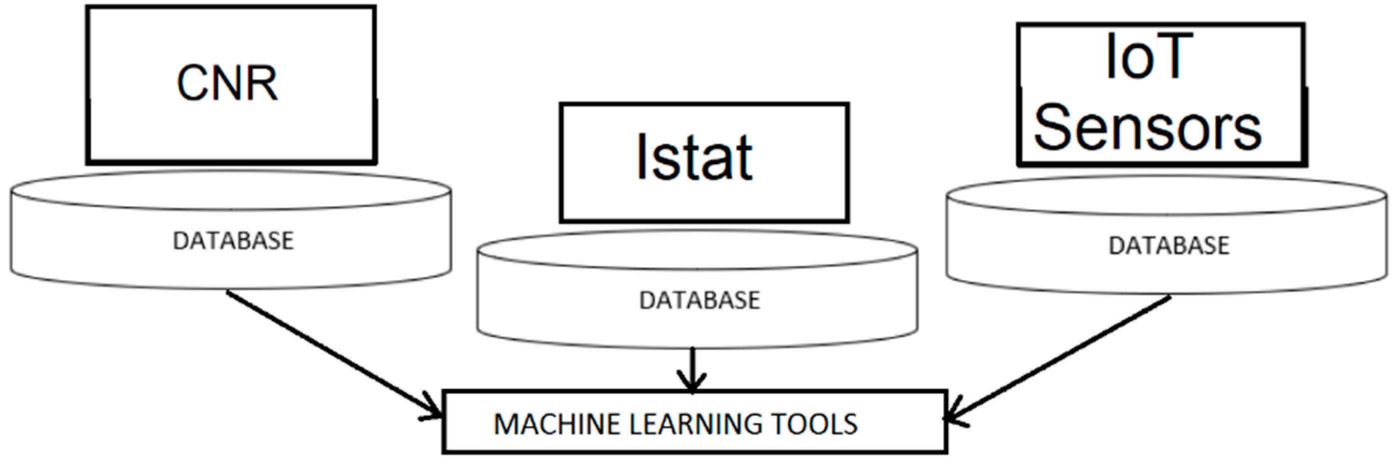
Funding

This work has been supported by the ECO-LOOP project (No. 2AT8246) funded by the Regione Puglia POR Puglia FESR—FSE 2014–2020. Fondo Europeo Sviluppo Regionale. Azione 1.6—Avviso pubblico “InnoNetwork”.

Acknowledgments

The computational work has been executed on the IT resources of the ReCaS-Bari data center, which have been made available by two projects financed by the MIUR (Italian Ministry for Education, University and Research) in the “PON Ricerca e Competitività 2007–2013” Program: ReCaS (Azione I—Interventi di rafforzamento strutturale, PONa3_00052, Avviso 254/Ric) and PRISMA (Asse II—Sostegno all’innovazione, PON04a2_A.

Conflicts of Interest

The authors declare no conflict of interest. The funders had no role in the design of the study; in the collection, analyses, or interpretation of data; in the writing of the manuscript; and in the decision to publish the results.

References

  1. IV Censimento Della Agricoltura. Available online: http://censimentoagricoltura.istat.it (accessed on 3 May 2018).
  2. Classificazione Delle Attività Agricole. Available online: http://www.codiciateco.it/coltivazioni-agricole-e-produzione-di-prodotti-animali--caccia-e-servizi-connessi/A-01 (accessed on 15 August 2018).
  3. Sundmaeker, H.; Verdouw, C.; Wolfert, S.; PrezFreire, L. Internet of Food and Farm 2020. In Digitising the Industry—Internet of Things Connecting Physical, Digital and Virtual Worlds; River Publishers: Gistrup, Denmark, 2016; Volume 2. [Google Scholar]
  4. Wolfert, S.; Ge, L.; Verdouw, C.; Bogaardt, M.-J. Big data in smart farming a review. Agric. Syst. 2017, 153, 69–80. [Google Scholar] [CrossRef]
  5. Biradarand, H.B.; Shabadi, L. Review on IoT based multidisciplinary models for smart farming. In Proceedings of the 2nd IEEE International Conference on Recent Trends in Electronics, Information Communication Technology (RTEICT), Bangalore, India, 19–20 May 2017; pp. 1923–1926. [Google Scholar]
  6. Ramya, R.; Sandhya, C.; Shwetha, R. Smart farming systems using sensors. In Proceedings of the 2017 IEEE Technological Innovations in ICT for Agriculture and Rural Development (TIAR), Chennai, India, 7–8 April 2017; pp. 218–222. [Google Scholar]
  7. Yoon, C.; Huh, M.; Kang, S.G.; Park, J.; Lee, C. Implement smart farm with IoT technology. In Proceedings of the 20th International Conference on Advanced Communication Technology (ICACT), Chuncheon-si Gangwon-do, Korea, 11–14 February 2018; pp. 749–752. [Google Scholar]
  8. Arkeman, Y.; Utomo, H.A.; Wibawa, D.S. Design of web-based information system with green house gas analysis for palm oil biodiesel agroindustry. In Proceedings of the 3rd International Conference on Adaptive and Intelligent Agroindustry (ICAIA), Bogor, Indonesia, 3–4 August 2015; pp. 238–244. [Google Scholar]
  9. Amanda, E.C.R.; Seminar, K.B.; Syukur, M.; Noguchi, R. Development of expert system for selecting tomato (Solanum lycopersicum L.) varieties. In Proceedings of the 3rd International Conference on Adaptive and Intelligent Agroindustry (ICAIA), Bogor, Indonesia, 3–4 August 2015; pp. 278–283. [Google Scholar]
  10. Nurulhaq, N.Z.; Sitanggang, I.S. Sequential pattern mining on hotspot data in Riau province using the prefixspan algorithm. In Proceedings of the 3rd International Conference on Adaptive and Intelligent Agroindustry (ICAIA), Bogor, Indonesia, 3–4 August 2015; pp. 257–260. [Google Scholar]
  11. Murphy, F.E.; Popovici, E.; Whelan, P.; Magno, M. Development of an heterogeneous wireless sensor network for instrumentation and analysis of beehives. In Proceedings of the 2015 IEEE International Instrumentation and Measurement Technology Conference (I2MTC), Pisa, Italy, 11–14 May 2015; pp. 346–351. [Google Scholar]
  12. Saha, A.K.; Saha, J.; Ray, R.; Sircar, S.; Dutta, S.; Chattopadhyay, S.P.; Saha, H.N. Iot-based drone for improvement of crop quality in agricultural field. In Proceedings of the IEEE 8th Annual Computing and Communication Workshop and Conference (CCWC), Las Vegas, NV, USA, 8–10 January 2018; pp. 612–615. [Google Scholar]
  13. Monsanto. Available online: https://monsanto.com/ (accessed on 3 May 2018).
  14. Farmlink. Available online: https://farmlink.net/ (accessed on 3 May 2018).
  15. Farmlogs. Available online: https://farmlogs.com/ (accessed on 3 May 2018).
  16. Lesser, A. Big Data and Big Agriculture; Gigaom Research: San Francisco, CA, USA, 2014. [Google Scholar]
  17. Patil, S.S.; Thorat, S.A. Early detection of grapes diseases using machine learning and IoT. In Proceedings of the 2nd International Conference on Cognitive Computing and Information Processing (CCIP), Mysore, India, 12–13 August 2016; pp. 1–5. [Google Scholar]
  18. Truong, T.; Dinh, A.; Wahid, K. An IoT environmental data collection system for fungal detection in crop fields. In Proceedings of the IEEE 30th Canadian Conference on Electrical and Computer Engineering (CCECE), Windsor, ON, Canada, 30 April–3 May 2017; pp. 1–4. [Google Scholar]
  19. Sarangdhar, A.A.; Pawar, V.R. Machine learning regression technique for cotton leaf disease detection and controlling using IoT. In Proceedings of the 2017 International Conference of Electronics, Communication and Aerospace Technology (ICECA), Coimbatore, India, 20–22 April 2017; Volume 2, pp. 449–454. [Google Scholar]
  20. Satamraju, K.P.; Shaik, K.; Vellanki, N. Rural bridge: A novel system for smart and co-operative farming using IoT architecture. In Proceedings of the 2017 International Conference on Multimedia, Signal Processing and Communication Technologies (IMPACT), Aligarh, India, 24–26 November 2017; pp. 22–26. [Google Scholar]
  21. Pallavi, S.; Mallapur, J.D.; Bendigeri, K.Y. Remote sensing and controlling of greenhouse agriculture parameters based on IoT. In Proceedings of the 2017 International Conference on Big Data, IoT and Data Science (BID), Pune, India, 20–22 December 2017; pp. 44–48. [Google Scholar]
  22. Kaloxylos, A.; Eigenmann, R.; Teye, F.; Politopoulou, Z.; Wolfert, S.; Shrank, C.; Dillinger, M.; Lampropoulou, I.; Antoniou, E.; Pesonen, L.; et al. Farm management systems and the future internet era. Comput. Electron. Agric. 2012, 89, 130–144. [Google Scholar] [CrossRef]
  23. Kaloxylos, A.; Groumas, A.; Sarris, V.; Katsikas, L.; Magdalinos, P.; Antoniou, E.; Politopoulou, Z.; Wolfert, S.; Brewster, C.; Eigenmann, R.; et al. A cloud-based farm management system: Architecture and implementation. Comput. Electron. Agric. 2014, 100, 168–179. [Google Scholar] [CrossRef]
  24. Poppe, K.; Wolfert, J.; Verdouw, C.; Renwick, A. A European perspective on the economics of big data. Farm Policy J. 2015, 12, 11–19. [Google Scholar]
  25. Garba, A. Smart water-sharing methods for farms in semi-arid regions. In Proceedings of the 2017 IEEE Technological Innovations in ICT for Agriculture and Rural Development (TIAR), Chennai, India, 7–8 April 2017; pp. 1–7. [Google Scholar]
  26. Hlaingand, C.S.; Zaw, S.M.M. Plant diseases recognition for smart farming using model-based statistical features. In Proceedings of the IEEE 6th Global Conference on Consumer Electronics (GCCE), Nagoya, Japan, 24–27 October 2017; pp. 1–4. [Google Scholar]
  27. Alipio, M.I.; Cruz, A.E.; Doria, J.D.; Fruto, R.M. A smart hydroponics farming system using exact inference in bayesian network. In Proceedings of the IEEE 6th Global Conference on Consumer Electronics (GCCE), Nagoya, Japan, 24–27 October 2017; pp. 1–5. [Google Scholar]
  28. Marimuthu, R.; Alamelu, M.; Suresh, A.; Kanagaraj, S. Design and development of a persuasive technology method to encourage smart farming. In Proceedings of the 2017 IEEE Region 10 Humanitarian Technology Conference (R10-HTC), Dhaka, Bangladesh, 21–23 December 2017; pp. 165–169. [Google Scholar]
  29. Tong, L.; Hong, T.; JingHua, Z. Research on the big data-based government decision and public information service model of food safety and nutrition industry. J. Food Saf. Qual. 2015, 6, 366–371. [Google Scholar]
  30. Venkatesan, R.; Tamilvanan, A. A sustainable agricultural system using IoT. In Proceedings of the 2017 International Conference on Communication and Signal Processing (ICCSP), Chennai, India, 6–8 April 2017; pp. 763–767. [Google Scholar]
  31. Bauer, J.; Aschenbruck, N. Design and implementation of an agricultural monitoring system for smart farming. In Proceedings of the 2018 IoT Vertical and Topical Summit on Agriculture—Tuscany (IOT Tuscany), Tuscany, Italy, 8–9 May 2018; pp. 1–6. [Google Scholar]
  32. Pandithurai, O.; Aishwarya, S.; Aparna, B.; Kavitha, K. Agro-tech: A digital model for monitoring soil and crops using internet of things (IoT). In Proceedings of the 3rd International Conference on Science Technology Engineering Management (ICONSTEM), Chennai, India, 23–24 March 2017; pp. 342–346. [Google Scholar]
  33. Roselin, A.R.; Jawahar, A. Smart agro system using wireless sensor networks. In Proceedings of the 2017 International Conference on Intelligent Computing and Control Systems (ICICCS), Madurai, India, 15–16 June 2017; pp. 400–403. [Google Scholar]
  34. Rekha, P.; Rangan, V.P.; Ramesh, M.V.; Nibi, K.V. High yield groundnut agronomy: An IoT based precision farming framework. In Proceedings of the 2017 IEEE Global Humanitarian Technology Conference (GHTC), San Jose, CA, USA, 19–22 October 2017; pp. 1–5. [Google Scholar]
  35. Li, P.; Wang, J. Research progress of intelligent management for greenhouse environment information. Trans. Chin. Soc. Agric. Mach. 2014, 45, 236–243. [Google Scholar]
  36. Zhou, M.; Wang, R.; Mai, S.; Tian, J. Spatial and temporal patterns of air quality in the three economic zones of China. J. Maps 2016, 12, 156–162. [Google Scholar] [CrossRef] [Green Version]
  37. Sun, Z.; Du, K.; Zheng, F. Research prospects in wisdom agriculture and application of large data. J. Agric. Sci. Technol. 2013, 15, 63–71. [Google Scholar]
  38. Impedovo, D.; Pirlo, G. Updating Knowledge in Feedback-Based Multi-classifier Systems. In Proceedings of the 2011 International Conference on Document Analysis and Recognition, Beijing, China, 18–21 September 2011; pp. 227–231. [Google Scholar]
  39. Verhoosel, J.; Bekkum, M.; Verwaart, T. Horticube: A Platform for Transparent, Trusted Data Sharing in the Food Supply Chain. Available online: http://centmapress.ilb.uni-bonn.de/ojs/index.php/proceedings/article/view/1642/0 (accessed on 3 May 2018).
  40. Kaishi, S.K. Big data analysis medical, agriculture, in the environmental field. Seibutsu-kogaku Kaishi 2014, 92, 92–93. [Google Scholar]
  41. Istat—National Institute of Statistics/CC-BY-SA-3.0. Available online: dati.istat.it/ (accessed on 3 May 2018).
  42. CNR—National Research Council/CC-BY-SA-3.0. Available online: http://data.cnr.it/site/data (accessed on 3 May 2018).
  43. Industrial IoT Sensors Dataset. Unpublished data. 2018.
  44. Junior, S.L.D.; Cecatto, J.R.; Fernandes, M.M.; Ribeiro, M.X. SeMiner: A Flexible Sequence Miner Method to Forecast Solar Time Series. Information 2018, 9, 8. [Google Scholar] [CrossRef]
  45. Ma, L.; Gu, X.; Wang, B. Correction of Outliers in Temperature Time Series Based on Sliding Window Prediction in Meteorological Sensor Network. Information 2017, 8, 60. [Google Scholar] [CrossRef]
Figure 1. The datasets used for this study: National Research Council (CNR) scientific dataset, Istat statistical dataset, and the industrial Internet of Things (IoT) Sensors dataset.
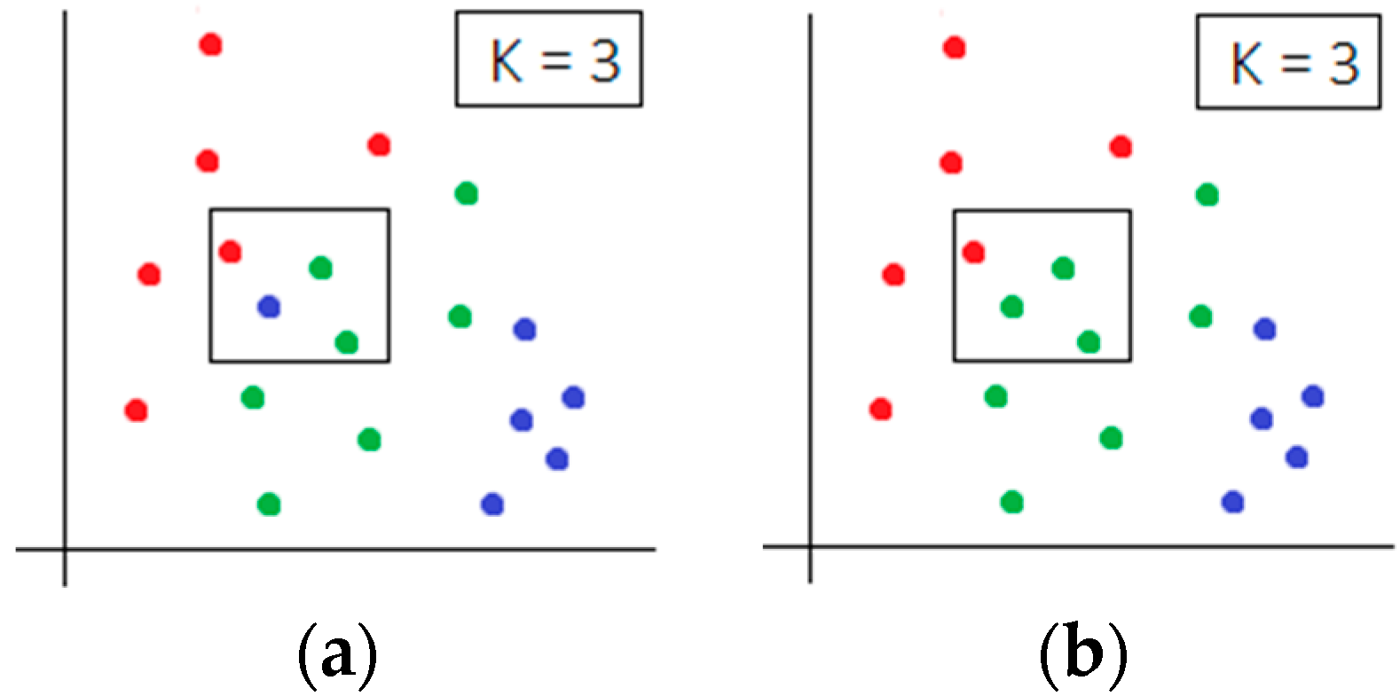
Machines 06 00038 g001
Figure 2. Two consecutive steps of the K-nearest neighbors (KNN) algorithm (K = 3) in a bi-dimensional feature space; (a): a blue item has ambiguous clustering, (b) the green cluster is assigned to it according to its number and proximity.
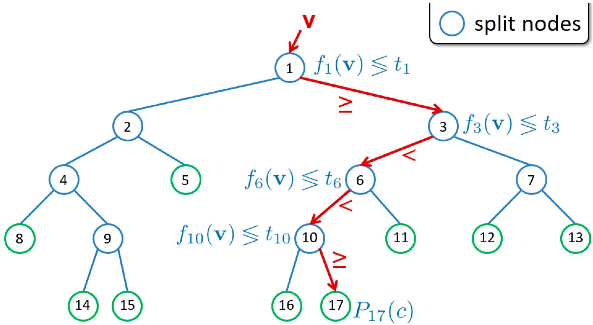
Machines 06 00038 g002
Figure 3. A (binary) decision tree used to classify and predict values with numerical features.
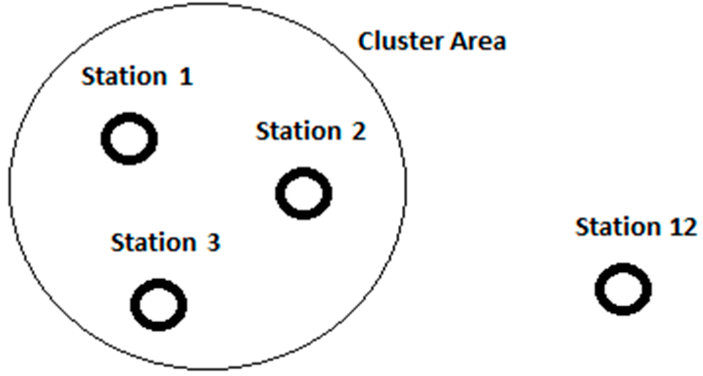
Machines 06 00038 g003
Figure 4. Task 4: the monitoring station clustering brings together geographically close sensors that are expected to record very similar data values.
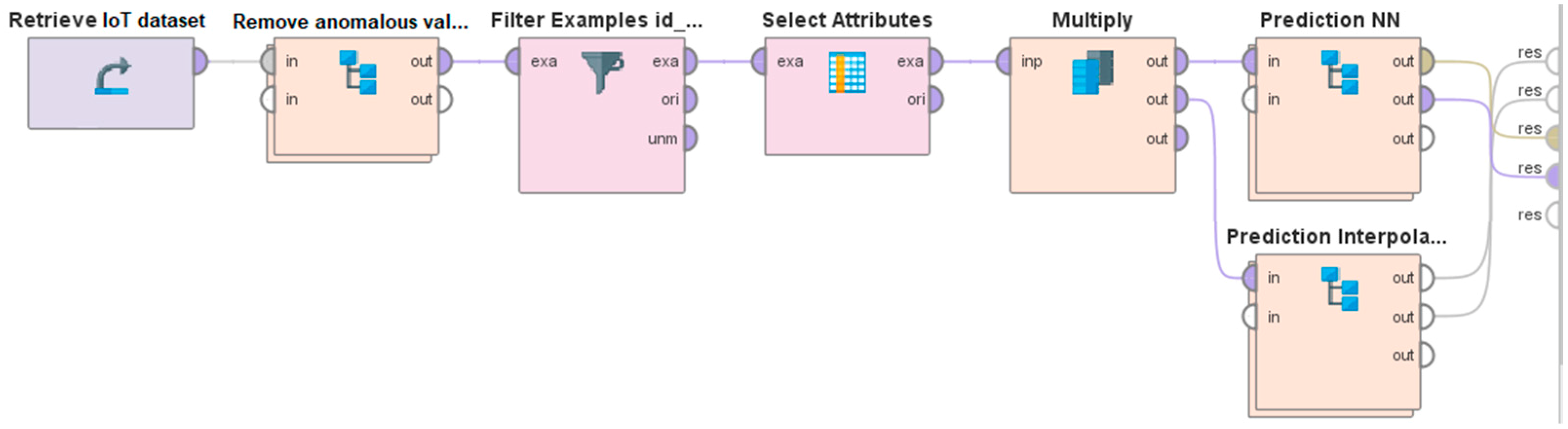
Machines 06 00038 g004
Figure 5. The workflow blocks on the IoT dataset featuring the two predictive models for the Task 3: the IoT sensors dataset is loaded, invalid and missing values are removed, there are filters to find the monitoring stations and the combination of their attributes, and finally the two machines learning sub-process blocks for the execution of the models.
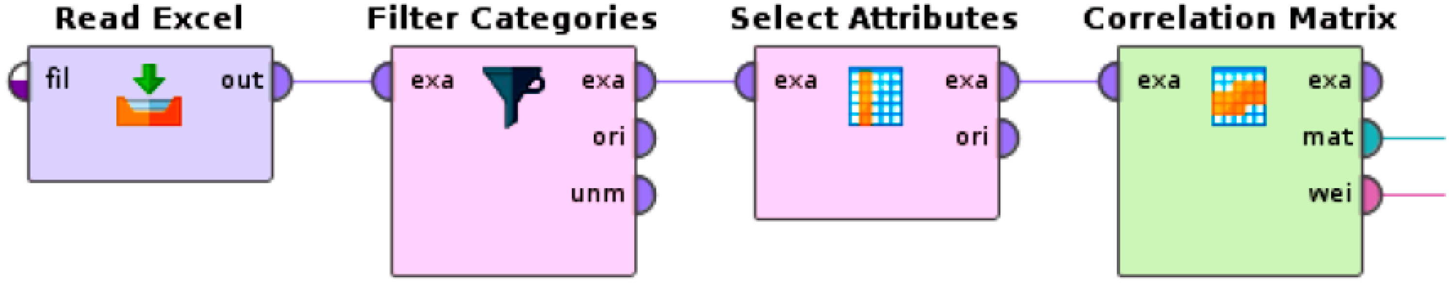
Machines 06 00038 g005
Figure 6. A workflow for a correlation matrix to visualize the attributes magnitude for Task 5, where the input dataset is the result of the monitoring stations clustering.
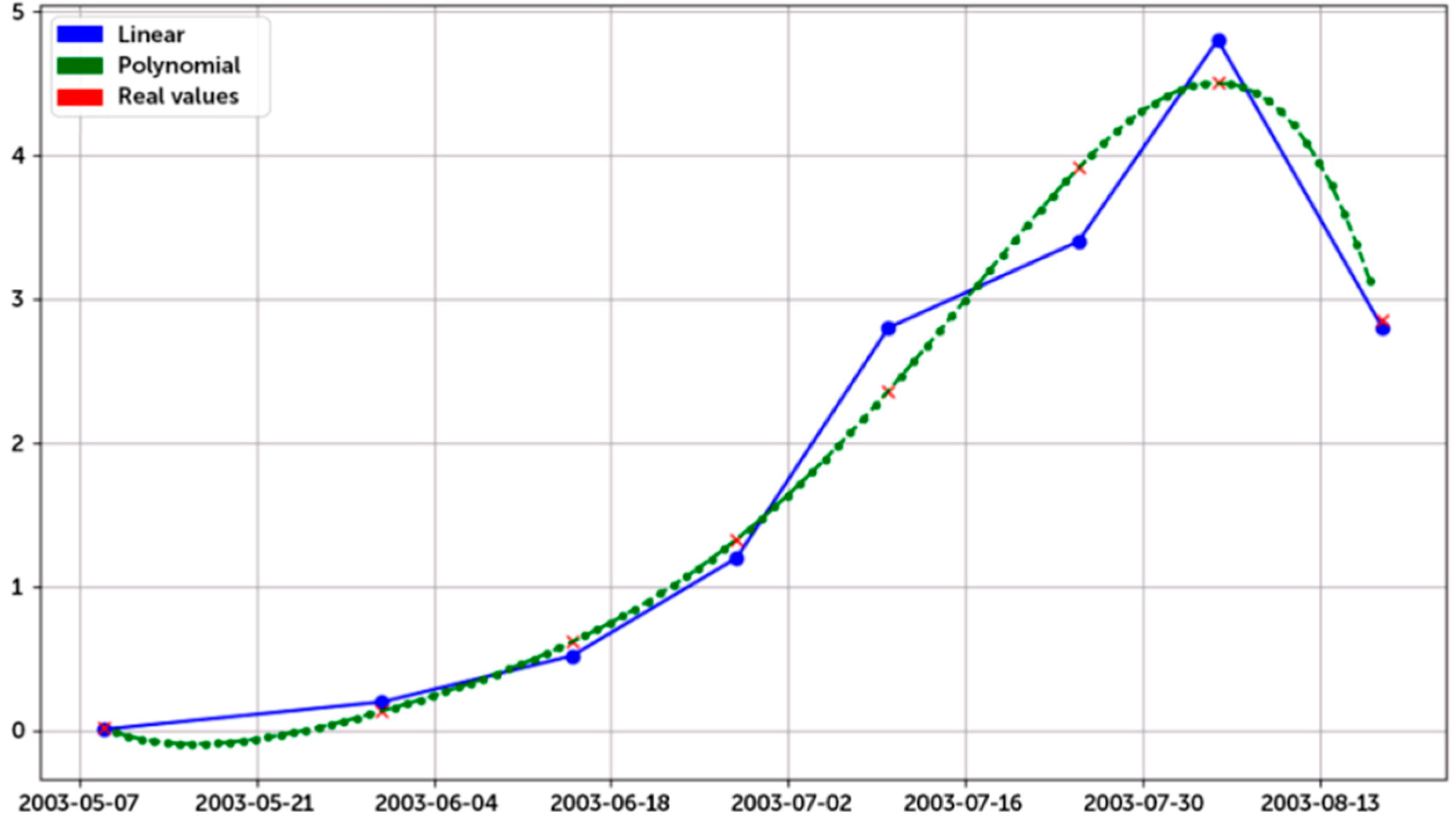
Machines 06 00038 g006
Figure 7. Task 2: plot comparison between real-values (red dots), the linear (blue), and polynomial (green) predictive model on the CNR scientific agrarian dataset.
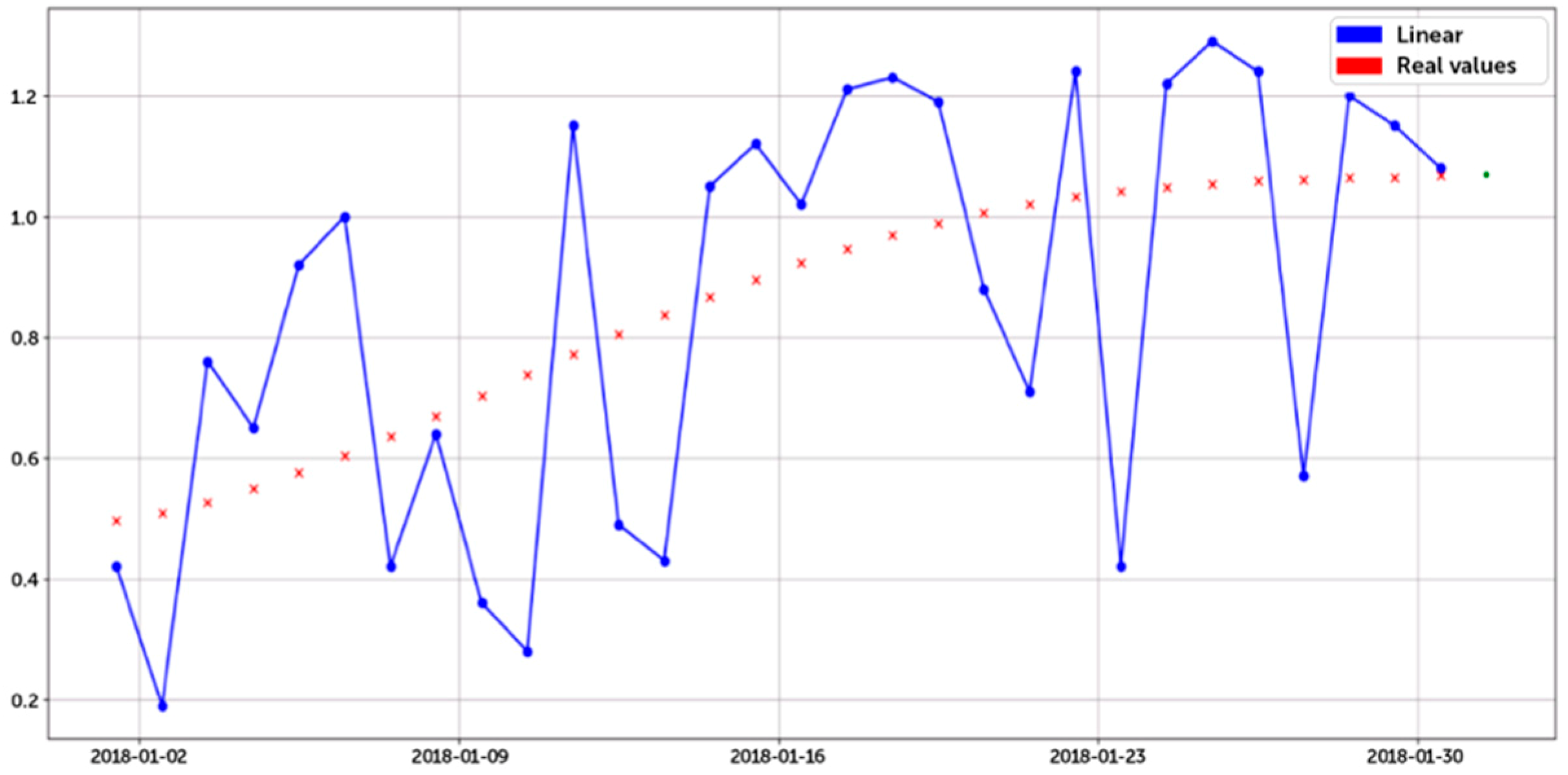
Machines 06 00038 g007
Figure 8. Task 3: sensor real-values (red dots) and their still insufficient linear predictive model (blue lines-at-step) employing a training time series of thirty days.
Machines 06 00038 g008
Table 1. Details about culture time-series in the Istat dataset.
Crop typeYearProvinceAltitudeTot. AreaCult. AreaTot. Prod.Tot. HarvestTemp. (Avg)
Apple2006Torino239928866264,240264,2407.6
Apple2006Vercelli13026264686468610
Temp. (Max)Temp. (Min)Tot. Rain.Phosph. MineralsPotash MineralsOrganic Fert.Organic Comp.
12.62.562322,312130,65111,731491,498
14.75.3644140447,61296,244280,932
Table 2. Details of the National Research Council (CNR) scientific agrarian dataset. LAI—leaf area index; ETc—evapotranspiration; ETo—evapotranspiration reference value; PM—Penman-Monteith.
Beamplant-2003 Crop
DateEtc (mm/d)ETo PM (mm/d)ETc/EToLAI
9 May 20031.194.80.250.01
11 May 20031.294.50.290.2
Table 3. Details of the Internet of Things (IoT) sensors dataset.
Id_StationPoiLatitudeLongitudeAltitudeDate_Time
46Cellino San Marco40.47561417.93942161.148 March 2015 12:50
46Cellino San Marco40.47561417.93942161.148 March 2015 13:04
r_incRainTminTmaxTmedRH_minRH_maxRH_medWSWdirPmed
\N0.0022.7022.7022.70\N\N25.60\N\N\N
\N0.0023.3023.3023.30\N\N23.10\N\N\N
Table 4. Task 1: apples and pears crop prediction error exploiting the neural network and the polynomial linear predictive model on the Istat dataset.
Italian ProvincePrediction Error—ApplePrediction Error—Pears
NNLRNNLR
Udine6.10%25.50%3.53%14.19%
Gorizia12.72%45.56%6.64%16.33%
Trieste21.80%21.25%9.83%21.25%
Pordenone12.04%38.47%154.79%153.12%
L’Aquila0.05%0.06%0.04%0.08%
Teramo2.52%2.53%1.52%13.03%
Pescara3.74%5.45%10.52%19.17%
Chieti3.65%10.54%2.26%2.73%
Cosenza22.68%63.79%16.57%20.62%
Catanzaro8.23%21.12%2.97%55.93%
Reggio Calabria11.38%42.60%6.14%13.08%
Crotone7.00%95.57%7.46%133.60%
Vibo Valentia7.50%27.55%29.40%45.31%
Mean9.19%30.77%19.36%39.11%
Table 5. Task 1: a comparison example between the real values and their neural network model prediction for the apple and pear total crops for the Italian province of L’Aquila on the Istat dataset.
Method: NNApplePears
Italian ProvinceReal ValuePredicted ValueReal ValuePredicted Value
L’Aquila45,90045,00039253750
Table 6. Task 2: comparison on the prediction error for the cultures leaf area index (LAI) value exploiting machine learning methods on the CNR scientific agrarian dataset.
CulturePrediction Error
NNLRPolynomial
Artichokes139.00%101.63%25.70%
Pear1779.38%81.80%10.00%
Pacciamata Eggplant933.10%564.89%6.26%
Table 7. Task 3: prediction error of the sensor attribute r_inc coming from monitoring station 173 using neural network, and linear and polynomial regression machine learning models on the IoT Sensors dataset.
Station: 173Prediction Error (Training: 1 January–30 January 2018)
FactorsNNLRPolynomial
BASE(r_inc + lat + lon + alt)53.7157.77469.78
BASE + Temp83.7042.55469.78
BASE + RH + Temp28.9128.80469.78
BASE + RH31.4025.54469.78
BASE + RH + Temp + Rain28.8228.80469.78
Table 8. Task 3: prediction error of the sensor attribute r_inc coming from monitoring station 186 using neural network, and linear and polynomial regression machine learning models on the IoT Sensors dataset.
Station: 186Prediction Error (Training: 1 January–30 January 2018)
FactorsNNLRPolynomial
BASE(r_inc + lat + lon + alt)105.37110.31526.33
BASE + Temp108.4173.77526.33
BASE + RH + Temp104.8450.10526.33
BASE + RH82.1560.17526.33
BASE + RH + Temp + Rain82.4250.10526.33
Table 9. Task 3: prediction error of the sensor attribute r_inc coming from both 173 and 186 monitoring station using neural network, and linear and polynomial regression machine learning models on the IoT Sensors dataset.
Station: 173 + 186Prediction Error (Training: 1 January–30 January 2018)
FactorsNNLRPolynomial
BASE(r_inc + lat + lon + alt)104.5285.21248.28
BASE + Temp78.7665.66248.28
BASE + RH + Temp76.1643.48248.28
BASE + RH51.7351.04248.28
BASE + RH + Temp + Rain85.0843.48248.28
Table 10. Task 3: prediction error of the sensor attribute r_inc coming from both 173 and 186 monitoring station using neural network, and linear and polynomial regression machine learning models trained with different time-series interval for the training on the IoT Sensors dataset.
Station: 173 + 186Prediction Error
Training IntervalPrediction TestNNLRPolynomial
1 January–30 January 201831 January 20187.38%17.36%25.22%
26 January–30 January 201831 January 20185.96%17.07%66.81%
1 January–4 January 2018;
6 January–9 January 2018
5 January 201822.18%13.83%9.37%
Table 11. Task 4: missing data prediction error of the sensor attribute r_inc from monitoring station 173 using decision trees, KNN, and polynomial machine learning methods on IoT Sensors dataset.
Station: 173Prediction Error (Training: 1 January–30 January 2018)
FactorsDTKNNPolynomial
BASE(r_inc + lat + lon + alt)56.2265.02469.78
BASE + Temp38.1048.26469.78
BASE + RH + Temp24.1142.71469.78
BASE + RH27.0742.71469.78
BASE + RH + Temp + Rain24.1142.71469.78
Table 12. Task 4: missing data prediction error of the sensor attribute r_inc from monitoring station 186 using decision trees, KNN, and polynomial machine learning methods on IoT Sensors dataset.
Station: 186Prediction Error (Training: 1 January–30 January 2018)
FactorsDTKNNPolynomial
BASE(r_inc + lat + lon + alt)117.80107.17526.33
BASE + Temp89.16104.14526.33
BASE + RH + Temp63.20104.84526.33
BASE + RH62.98104.84526.33
BASE + RH + Temp + Rain69.82104.84526.33
Table 13. Task 4: missing data prediction error of the sensor attribute r_inc from both monitoring station 173 and 186 using decision trees (DT), KNN, and polynomial machine learning methods on IoT Sensors dataset.
Station: 173 + 186Prediction Error (training: 1 January–30 January 2018)
FactorsDTKNNPolynomial
BASE(r_inc + lat + lon + alt)68.7471.01248.28
BASE + Temp86.0485.17248.28
BASE + RH + Temp39.5380.12248.28
BASE + RH41.4480.12248.28
BASE + RH + Temp + Rain40.1280.12248.28
Table 14. Task 4: prediction error of the sensor attribute r_inc coming from both 173 and 186 monitoring station using decision tree, KNN, and polynomial regression machine learning models trained with different time-series interval for the training on the IoT Sensors dataset.
Station: 173 + 186Prediction Error
Training IntervalPrediction TestDTKNNPolynomial
1 January–30 January 201831 January 201812.109.6625.22
26 January–30 January 201831 January 201829.377.6566.81
1 January–4 January 2018;
6 January–9 January 2018
5 January 201822.3816.169.37
Table 15. Task 5: a cluster of three monitoring stations where the high value of the difference_max on the r_inc attribute indicates a hardware sensor issue from June 2017 for the station 396.
r_inc (Station 394)r_inc (Station 396)r_inc (Station 397)Date_TimeDiff_Max
3.7400.5703.4309 June 2017 2:00:00 p.m.3.170
3.6100.4703.32014 June 2017 2:00:00 p.m.3.140
Table 16. Task 5: the correlation matrix for the clustering attributes magnitude.
Attributesr_incTminTmaxTmedRH_minRH_maxRH_medWS
r_inc10.0770.3510.213−0.739−0.431−0.2320.114
Tmin0.07710.9450.986−0.361−0.346−0.6460.098
Tmax0.3510.94510.985−0.638−0.463−0.6670.097
Tmed0.2130.9860.9851−0.525−0.441−0.6660.099
RH_min−0.739−0.3610.638−0.52510.5890.896−0.016
RH_max−0.431−0.346−0.463−0.4410.58910.777−0.055
RH_med−0.232−0.646−0.667−0.6660.8960.7771−0.339
WS0.1140.0980.0970.099−0.016−0.055−0.3391

