Shape-Regularized Meta-Learning Method for Performance Assessment of Solid Rocket Motors

Abstract

During the early developmental stages of solid rocket motors (SRMs), particularly under extreme operating conditions, the scarcity of experimental data severely limits the predictive capabilities of conventional deep learning models. To address this challenge, this paper proposes a novel hybrid predictive framework, termed Shape-Regularized Meta-Variational Multi-Scale Network (SR-MVSNet), tailored for few-shot thrust prediction via shape-regularized meta-learning. First, a variational autoencoder (VAE) maps nine static design and operating parameters to a latent probability distribution and reconstructs the parameter vector. A parallel multi-scale convolutional neural network (MSCNN) then processes the reconstructed features to predict the complete thrust curve. Crucially, a joint loss function with shape regularization is integrated within the model-agnostic meta-learning (MAML) architecture, guiding the network to reproduce the measured thrust build-up and decay through supervised first- and second-order difference matching. Experimental results demonstrate that the proposed framework achieves the lowest mean squared error among the evaluated models in the low-temperature-to-ambient-temperature transfer task. Notably, during the critical steady-state combustion phase, the mean absolute percentage error is 1.71% under the combined-source task, supporting accurate steady-state thrust prediction for the rapid performance evaluation of SRMs in engineering applications.

1. Introduction

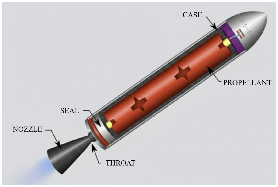
Solid rocket motors (SRMs) are crucial components of aerospace propulsion systems, extensively utilized in tactical missiles, launch vehicles, and deep space exploration missions due to their structural simplicity, high reliability, and excellent storability [1]. Accurately predicting the thrust performance of SRMs is critical, as it directly influences flight trajectory planning, structural reliability verification, and overall mission success, while also significantly reducing development costs [2,3]. Figure 1 illustrates the schematic configuration of an SRM, highlighting essential components such as the propellant grain, nozzle, and throat.

Traditionally, thrust prediction for SRMs has predominantly relied on three categories of conventional methods. The first category comprises theoretical calculation approaches grounded in combustion dynamics and internal ballistics. While these methods possess a solid physical foundation, they require highly precise physical parameters and struggle to adequately incorporate the complexities of real-world combustion environments [4,5]. The second category consists of numerical simulation techniques, such as computational fluid dynamics (CFD), which resolve the combustion flow field. However, these approaches frequently incur prohibitive computational costs and exhibit significant sensitivity to the specification of initial and boundary conditions [6,7,8]. The third category encompasses data-driven empirical methods that analyze extensive historical experimental data using statistical techniques. Despite their computational efficiency, their capacity to handle unseen samples is significantly constrained, making adaptation to novel requirements under varying operating conditions highly challenging [9].

For instance, the numerical study in [10] utilized CFD to predict the flow field during the boost and sustain phases, validating the numerical model by comparing numerical, analytical, and experimental thrust data. Although the authors successfully conducted numerical simulations for a specific dual-thrust SRM nozzle under two distinct high-pressure conditions, their reliance on a 2D steady-state axisymmetric model inherently disregarded the 3D characteristics and transient dynamics of the actual flow field. Furthermore, Li et al. [11] introduced the concept of modular grain design, formulating a least-squares objective function through geometric relationship analysis of the burnback characteristics and internal ballistic performance. The Nelder–Mead simplex method was employed to minimize the discrepancy between the calculated and target thrust curves. Nevertheless, this optimization remains contingent upon classical theoretical models of internal ballistics, which inherently fail to capture the complexities and transient phenomena of the actual combustion flow field. To model the dynamic combustion process, Carvalho [12] employed the quasi-steady-state (QSS) approach for numerical modeling to address the evolving geometry of the combustion chamber over time. This approach approximates the unsteady-state process by solving successive steady-state CFD simulations, where the combustion rate and geometry updates rely on the steady-state solution from the preceding phase. Consequently, if the time step is excessively large, numerical errors can compound significantly over time.

In summary, while conventional techniques for predicting SRM thrust have been extensively applied and validated in engineering practice, their inherent limitations continue to restrict predictive accuracy and computational efficiency. Consequently, there is an urgent need to explore novel, intelligent alternatives. To address the challenges of few-shot scenarios and distribution shifts across operating conditions, the hybrid deep learning framework proposed in this study offers an innovative theoretical and technical solution. Experimental results indicate that this method achieves accurate steady-state thrust prediction in the combined-source task, providing a data-driven technical pathway for SRM thrust evaluation. The primary contributions of this research are summarized as follows:

(1)

A novel hybrid prediction framework based on model-agnostic meta-learning (MAML) is proposed. Termed SR-MVSNet, this architecture integrates a variational autoencoder (VAE) with a multi-scale convolutional neural network (MSCNN) to improve thrust prediction with limited target-condition data.

(2)

A meta-task construction strategy tailored for unseen operating conditions is introduced. To overcome the scarcity of data under extreme environments and the significant distribution shifts across different batches, this strategy leverages auxiliary operating data to achieve efficient knowledge transfer to the target conditions.

(3)

A joint loss function with shape regularization is formulated. To capture the local variation in the thrust curve, the network is guided to match the first- and second-order differences of the measured thrust profile during training. This formulation incorporates local thrust-evolution information into the learning objective alongside pointwise prediction error.

The remainder of this paper is structured as follows. Section 2 outlines the related research, while Section 3 provides a detailed description of the SR-MVSNet architecture. Section 4 delineates the experimental setup and parameter configurations. Section 5 elucidates the model’s predictive outcomes on a multi-condition dataset and benchmarks them against established methodologies, and Section 6 encapsulates the conclusions of this research.

2. Related Research

In recent years, the rapid development of deep learning has enabled data-driven thrust prediction methods to demonstrate superior accuracy compared to traditional approaches, particularly in data-rich environments, by establishing end-to-end nonlinear mapping models. These models can automatically capture the complex nonlinear correlations between input parameters and thrust outputs [13,14,15,16]. For instance, Yang et al. [17] developed an enhanced ConvNeXt neural network to model the correlation between empirical parameters and ignition pressure data. Their key innovation was the implementation of a layer-freezing strategy, where specific model layers were frozen while an optimizer refined two critical empirical parameters within the turbulence model. Similarly, Yang et al. [18] introduced a Convolutional Neural Network (CNN) integrated with Long Short-Term Memory (LSTM) units and an attention mechanism, successfully predicting the total impulse of solid rockets using ignition thrust data. In the broader context of time-series modeling, Huang et al. [19] utilized LSTM units and Graph Convolutional Networks (GCNs) to effectively capture long-term temporal dependencies in traffic data, addressing the limitations of traditional GCNs.

Despite these notable advancements, thrust prediction for solid rocket motors continues to face the dual challenges of data scarcity and significant distribution shifts. On one hand, the prohibitive costs and destructive nature of experiments result in a scarcity of data during the early development phases, particularly for critical data under extreme conditions [20,21,22]. On the other hand, the data demonstrates pronounced multi-source heterogeneity due to variations in propellant formulation and nozzle design across batches, which substantially restricts the generalization capability of conventional models [23,24]. To address the modeling difficulties inherent in few-shot settings, meta-learning has garnered significant interest. Huisman et al. [25] and Tian et al. [26] demonstrated that gradient-based meta-learning techniques can rapidly adapt to novel tasks with minimal iterations. Mu et al. [27] proposed a task-oriented meta-learning network with a gradient calibration technique, effectively addressing the challenge of intelligent defect diagnosis in rotating equipment under constrained sample conditions. Complementing these empirical studies, Jose and Simeone [28] analyzed the generalization gap of meta-learning through the lens of information theory, offering substantial theoretical underpinning for the concept.

To further enhance the model’s capacity for capturing complex physical features and data distributions, researchers have increasingly investigated the integration of Variational Autoencoders with meta-learning. For example, Moon et al. [29] employed a VAE as their backbone model and implemented model-agnostic meta-learning (MAML) strategies to rapidly adapt to new sensor data, achieving sustained high performance even with limited sample sizes and outperforming existing state-of-the-art methodologies on real building sensor datasets. Cinelli et al. [30] formalized the fundamental role of VAEs in generative machine learning. Building on this, Lee et al. [31] proposed using a Gaussian Mixture Model (GMM) as the prior distribution within the VAE framework, optimized through the Expectation Maximization (EM) algorithm, demonstrating superior performance compared to established unsupervised baselines in few-shot classification tests. Negri et al. [32] introduced a pseudo-input prior based on model-agnostic meta-learning. This method parameterizes the prior distribution of the VAE using a neural network transformation of pseudo-inputs, employing a meta-learning mechanism for optimization to obtain richer and more hierarchical latent representations. Berti et al. [33] further enhanced the feature representation capacity of VAEs within the meta-learning framework through hyperparameter optimization. Furthermore, to address more complex reasoning and generation tasks, Gordon et al. [34] proposed a framework for meta-learning approximate probabilistic inference for prediction (ML-PIP) and introduced the versatile amortized inference (VERSA) algorithm. This approach directly maps few-shot datasets to the distribution of task-specific parameters, bypassing the gradient optimization process typically required during testing. Qi and Yu [35] and Zhang et al. [36] respectively incorporated causal mechanisms and conditional constraints, developing the causal meta variational autoencoder (CMVAE) and meta conditional variational autoencoder (MCVAE), which significantly improved model performance in unsupervised settings.

While the aforementioned studies established the theoretical foundation in general domains, recent research has begun to demonstrate the efficacy of VAEs specifically in aerospace propulsion. For instance, Xu et al. [37] utilized a Multi-channel VAE (MVAE) to cluster high-speed photography time-series data in a scramjet combustor, highlighting the robust capability of VAEs in extracting latent patterns from complex turbulent flames. Similarly, Zapata Usandivaras et al. [38] applied deep convolutional autoencoders for the spatiotemporal reconstruction of liquid rocket engine flames, validating the effectiveness of generative models in dimensionality reduction for combustion flow fields. In the context of fault detection, Zhu et al. [39] combined convolutional autoencoders with one-class support vector machines to detect steady-state faults in liquid rocket engines. Of particular relevance to this study, Lu et al. [40] proposed a Physics-Guided VAE-CNN state space model for predicting compressor cylinder pressure dynamics by explicitly embedding physical constraints into the VAE latent space to ensure physically consistent predictions. Additionally, Gong et al. [41] developed an improved dynamical VAE framework for predicting the remaining useful life of aero-engines.

Despite these significant advancements, thrust prediction for Solid Rocket Motors (SRMs) remains underexplored, particularly within the context of shape-regularized meta-learning. Existing applications in aerospace propulsion predominantly focus on fault diagnosis or flow field reconstruction for liquid rocket engines or scramjets, leaving a critical gap in unified frameworks capable of simultaneously addressing few-shot data scarcity, cross-condition distribution shifts, and the reconstruction of local thrust-curve shape. Consequently, this study proposes a novel hybrid deep learning framework, termed SR-MVSNet. This framework integrates supervised thrust-shape regularization with the representation of SRM design and operating parameters, establishing a robust architecture that synergizes deep feature extraction, time-series modeling, and meta-knowledge transfer.

3. Methods

3.1. Model-Agnostic Meta-Learning

3.1.1. Explanation on MAML

MAML learns an initialization from a collection of meta-training tasks $\mathcal{T}=\{T_1,T_2,\dots ,T_n\}$. In this study, each task is sampled within a source temperature domain, and multiple tasks can be constructed from the same domain. Each task $T_i$ contains a support set $S_i$ for inner-loop adaptation and a query set $Q_i$ for the outer-loop update:

$$S_i={\left\{({\mathbf{x}}_{i,r}^S,{\mathbf{y}}_{i,r}^S)\right\}}_{r=1}^K,Q_i={\left\{({\mathbf{x}}_{i,r}^Q,{\mathbf{y}}_{i,r}^Q)\right\}}_{r=1}^M.$$

(1)

Here, $\mathbf{x}\in {\mathbb{R}}^9$ denotes the input parameter vector and $\mathbf{y}\in {\mathbb{R}}^{440}$ denotes the corresponding thrust curve. The index i identifies a meta-training task, while K and M are its support and query sample counts. Section 5.3 evaluates transfer to the target domain using three source-domain configurations.

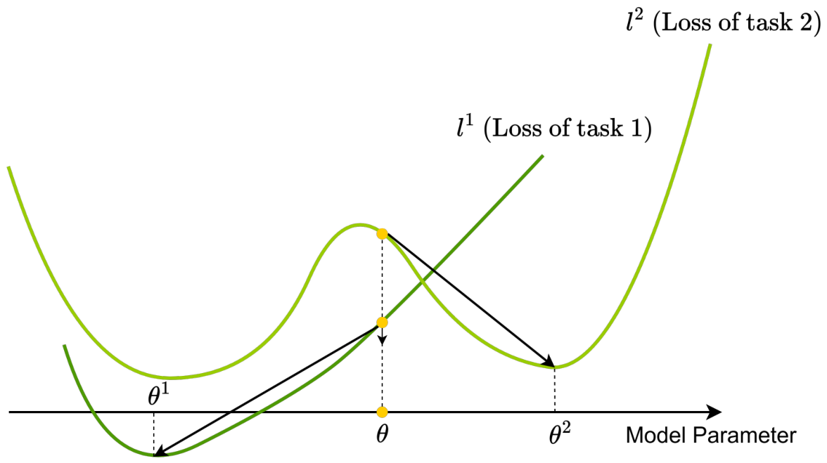
As illustrated in Figure 2, $\theta$ denotes the shared initialization parameters. For example, meta-training tasks sampled from the high- and low-temperature domains provide losses $l^1$ and $l^2$ for adaptation to task-specific parameters ${\theta }^1$ and ${\theta }^2$. The outer-loop update uses the source-task query losses to refine the shared initialization for subsequent adaptation to the ambient-temperature target domain.

The core objective of MAML is to identify an optimal set of global initialization parameters $\theta$, such that when the model encounters novel operating conditions, it can achieve minimal prediction error on the query set $Q_i$ with only a few gradient updates on the support set $S_i$. In this study, we leverage this strategy to enable the rapid adaptation of the predictive model from known to unseen operating environments.

3.1.2. Joint Loss Function with Shape Regularization

To achieve high numerical accuracy while capturing the local variation in solid rocket motor thrust curves, this paper formulates a joint loss function with shape regularization $L_{\mathrm{joint}}$. This composite objective function integrates mean squared error (MSE), supervised shape-matching terms, and variational regularization. Specifically, it penalizes discrepancies between predicted and measured first- and second-order differences, together with input reconstruction error and Kullback–Leibler (KL) divergence from the latent distribution to its prior. The joint loss function is used in both inner-loop adaptation and fine-tuning on target conditions, and is defined as follows:

$$L_{\mathrm{joint}}=L_{\mathrm{MSE}}+{\lambda }_s{L}_{\mathrm{slope}}+{\lambda }_c{L}_{\mathrm{curv}}+{\lambda }_r{L}_{\mathrm{recon}}+{\beta }_{\mathrm{KL}}{L}_{\mathrm{KL}}$$

(2)

where ${\lambda }_s$, ${\lambda }_c$, ${\lambda }_r$ and ${\beta }_{\mathrm{KL}}$ are the weight coefficients of each component. Through this joint optimization approach, the model balances pointwise prediction accuracy, local curve-shape matching, and variational feature learning under limited sample conditions.

The regression loss measures the mean squared error (MSE) between the whole thrust curve $\widehat{y}$ produced by the model and the measured test curve y, providing pointwise supervision for numerical prediction. The formula for its expression is as follows:

$$L_{\mathrm{MSE}}={\displaystyle \frac{1}{T}}{\displaystyle \sum _{t=1}^T}{\left({\widehat{y}}_t-y_t\right)}^2$$

(3)

where T is the output sequence’s length.

The local rise and decline of the thrust curve characterize the ignition and tail-off phases. This study uses a slope-matching regularization term that aligns the first-order differences of the predicted and measured curves, guiding the model to reproduce these local changes. Differences are evaluated over the retained sample indices. The precise definition is as follows:

$$L_{\mathrm{slope}}={\displaystyle \frac{1}{T-1}}{\displaystyle \sum _{t=1}^{T-1}}{\left|\left({\widehat{y}}_{t+1}-{\widehat{y}}_t\right)-\left(y_{t+1}-y_t\right)\right|}^2$$

(4)

The curvature-matching term complements first-order difference matching by aligning the second-order differences of the predicted and measured thrust curves. It penalizes discrepancies in how adjacent thrust increments change, encouraging the predicted curve to reproduce the local shape of the measured reference, including the steady-state region. The precise definition is as follows:

$$L_{\mathrm{curv}}={\displaystyle \frac{1}{T-2}}{\displaystyle \sum _{t=1}^{T-2}}{\left|\left({\Delta }^2{\widehat{y}}_t\right)-\left({\Delta }^2{y}_t\right)\right|}^2$$

(5)

where ${\Delta }^2{y}_t=\left(y_{t+2}-y_{t+1}\right)-\left(y_{t+1}-y_t\right)$.

3.1.3. MAML Algorithm Process

The complete meta-learning procedure is summarized in Algorithm 1. In the inner loop, for any task $T_i$, the model parameters are updated using the support set loss function $L_{\mathrm{joint}}$:

$${\theta }_i^{\prime }=\theta -\alpha {\nabla }_{\theta }{L}_{\mathrm{joint}}\left(\theta ;S_i\right)$$

(6)

where $\alpha$ is the learning rate of the inner loop. This paper introduces the joint loss function with shape regularization in the inner loop to guide the model toward matching both measured thrust values and local curve shape during rapid adaptation. Subsequently, the loss is computed on the query set using the adapted parameters ${\theta }_i^{\prime }$, followed by a meta-update of the global parameters, as follows:

$$\theta \leftarrow \theta -\beta {\nabla }_{\theta }\sum _i{L}_{\mathrm{outer}}\left(f_{{\theta }_i^{\prime }};Q_i\right)$$

(7)

where $\beta$ is the outer-loop learning rate. Crucially, shape regularization in the inner loop provides additional supervision during few-shot fine-tuning. Conversely, the use of MSE together with slope- and curvature-matching terms in the outer loop ensures predictive accuracy, guiding the meta-parameters to converge toward a robust configuration that accurately reflects the operating conditions. The outer-loop objective is $L_{\mathrm{outer}}=L_{\mathrm{MSE}}+{\lambda }_s{L}_{\mathrm{slope}}+{\lambda }_c{L}_{\mathrm{curv}}$. The inner-loop and target-domain fine-tuning objectives additionally include VAE reconstruction and KL regularization.  

Algorithm 1 Meta-learning stage

1: Input: Tasks $\{S_i,Q_i\}$, learning rates $\alpha ,\beta$   2: Output: Optimized meta-parameters $\theta$   3: Initialize global parameters $\theta$   4: while not converged do   5:     Sample a batch of tasks $T_i$   6:     for each task $T_i$ do   7:         Evaluate joint loss on Support Set $S_i$   8:         Update task-specific parameters: ${\theta }_i^{\prime }=\theta -\alpha {\nabla }_{\theta }{L}_{\mathrm{joint}}(\theta ;S_i)$   9:         Evaluate regression performance on Query Set $Q_i$ using ${\theta }_i^{\prime }$: 10:         $L_{\mathrm{meta}}^i=L_{\mathrm{outer}}(f_{{\theta }_i^{\prime }};Q_i)$ 11:     end for 12:     $\theta \leftarrow \theta -\beta {\nabla }_{\theta }{\sum }_i{L}_{\mathrm{meta}}^i$ 13: end while 14: Adapt $\theta$ to target condition using $S_{\mathrm{target}}$ and $L_{\mathrm{joint}}$ to obtain $f_{{\theta }^{*}}$

3.2. Variational Auto-Encoder

In this framework, the VAE encodes the nine normalized design and operating parameters into a probabilistic latent representation. The encoder produces an 80-dimensional latent variable, and the decoder reconstructs the nine-dimensional input vector. The reconstructed parameters are then passed to the MSCNN for thrust prediction. Stochastic latent sampling introduces feature-level variation during training.

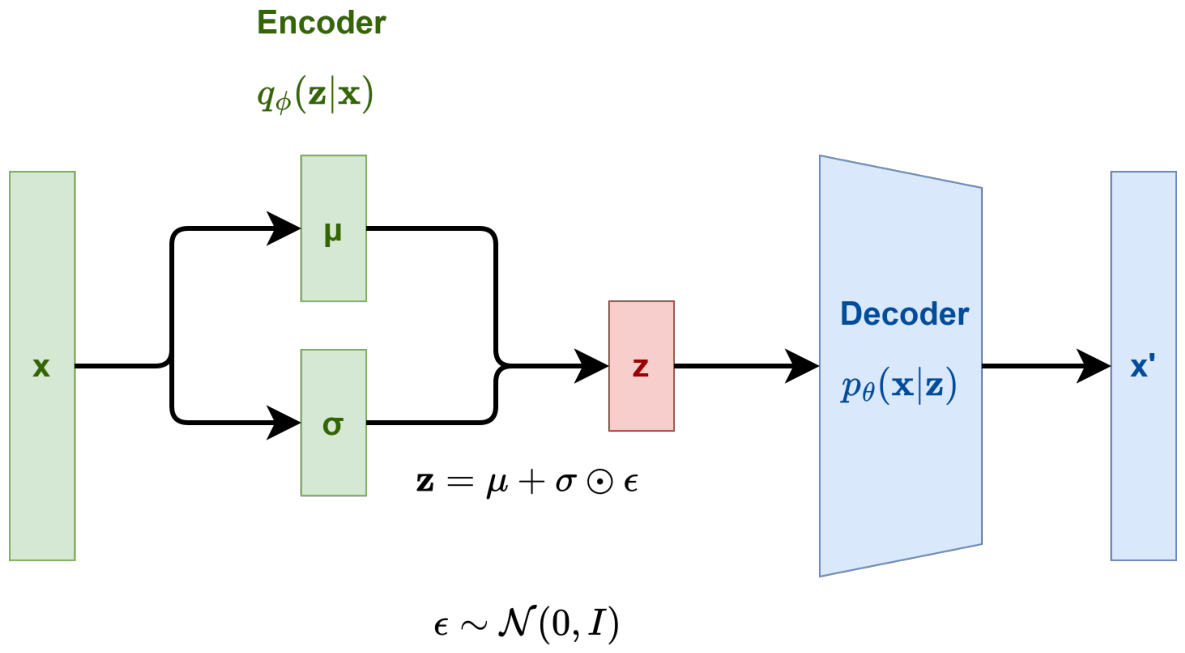
Figure 3 illustrates the VAE encoder and decoder. The input $\mathbf{x}\in {\mathbb{R}}^9$ contains the normalized static design and operating parameters. The encoder approximates $q_{\varphi }(\mathbf{z}\mid \mathbf{x})$, and the decoder reconstructs ${\mathbf{x}}^{\prime }\in {\mathbb{R}}^9$ from the latent variable through $p_{\theta }(\mathbf{x}\mid \mathbf{z})$. The downstream regression network uses the reconstructed parameters to predict the measured thrust curve. The encoder maps the normalized parameter vector to the mean $\mathit{\mu }$ and log-variance $\log {\mathit{\sigma }}^2$ of the latent distribution. These quantities describe the learned feature distribution conditional on the input parameters. The reparameterization trick expresses a latent sample using an auxiliary standard-normal noise vector $\mathit{ϵ}$, allowing gradients to propagate through $\mathit{\mu }$ and $\mathit{\sigma }$ as follows:

$$\mathbf{z}=\mathit{\mu }+\mathit{ϵ}\odot \mathit{\sigma }$$

(8)

Algorithm 2 details the operational procedure of the VAE. Since the variance ${\mathit{\sigma }}^2$ must strictly be positive, directly predicting it can lead to numerical instability. To address this, the network predicts the logarithmic variance $\log {\mathit{\sigma }}^2$, and the standard deviation is subsequently recovered via exponential transformation.

Algorithm 2 VAE for SRM Feature Extraction and Data Augmentation

1: Input: Normalized parameter vector $\mathbf{x}\in {\mathbb{R}}^9$; Augmentation flag use_aug; Sample size N   2: Output: Reconstructed features: N vectors with augmentation, or one vector otherwise   3: $\mathit{\mu },\log {\mathit{\sigma }}^2\leftarrow {\mathrm{Encoder}}_{\varphi }\left(\mathbf{x}\right)$   4: $\mathit{\sigma }\leftarrow \exp (0.5\times \log {\mathit{\sigma }}^2)$   5: $L_{\mathrm{KL}}\leftarrow -0.5\sum (1+\log {\mathit{\sigma }}^2-{\mathit{\mu }}^2-\exp \left(\log {\mathit{\sigma }}^2\right))$   6: if use_aug is True then   7:     for $k\leftarrow 1$ to N do   8:         Sample ${\mathit{ϵ}}_k\sim \mathcal{N}(0,\mathbf{I})$   9:         ${\mathbf{z}}_k\leftarrow \mathit{\mu }+{\mathit{ϵ}}_k\odot \mathit{\sigma }$ 10:         ${\mathbf{x}}_k^{\prime }\leftarrow {\mathrm{Decoder}}_{\theta }\left({\mathbf{z}}_k\right)$ 11:     end for 12:     $L_{\mathrm{recon}}\leftarrow {\displaystyle \frac{1}{N}}{\sum }_{k=1}^N{\parallel \mathbf{x}-{{\mathbf{x}}^{\prime }}_k\parallel }^2$ 13:     return ${\left\{{{\mathbf{x}}^{\prime }}_k\right\}}_{k=1}^N$ 14: else 15:     Sample $\mathit{ϵ}\sim \mathcal{N}(0,\mathbf{I})$ 16:     $\mathbf{z}\leftarrow \mathit{\mu }+\mathit{ϵ}\odot \mathit{\sigma }$ 17:     ${\mathbf{x}}^{\prime }\leftarrow {\mathrm{Decoder}}_{\theta }\left(\mathbf{z}\right)$ 18:     $L_{\mathrm{recon}}\leftarrow {\parallel \mathbf{x}-{\mathbf{x}}^{\prime }\parallel }^2$ 19:     return ${\mathbf{x}}^{\prime }$ 20: end if

During the sampling process, an auxiliary noise variable $\mathit{ϵ}$ is drawn from a standard normal distribution. The predicted mean $\mathit{\mu }$ serves as the deterministic centroid of the latent representation. By combining $\mathit{ϵ}$ with the uncertainty scale $\mathit{\sigma }$, a stochastic latent feature vector $\mathbf{z}$ is sampled from the latent space via the reparameterization trick ($\mathbf{z}=\mathit{\mu }+\mathit{ϵ}\odot \mathit{\sigma }$). Subsequently, the decoder generates the kth reconstructed sample ${\mathbf{x}}_k^{\prime }$ from ${\mathbf{z}}_k$.

The VAE objective contains a regularization term $L_{\mathrm{KL}}$ and a reconstruction term $L_{\mathrm{recon}}$. The KL term compares the learned latent distribution with the standard normal prior. The reconstruction term compares the reconstructed nine-dimensional parameter vector with its normalized input. Thrust prediction error is evaluated separately against the measured thrust target in the joint training objective.

3.3. Multi-Scale Convolutional Neural Networks

The MSCNN maps the reconstructed parameter vector to the complete thrust curve. Its input tensor X has shape $[B,1,9]$, where B is the batch size, the middle dimension denotes one input channel, and the length-nine axis follows the fixed order of the input variables. Parallel one-dimensional convolutional branches operate over different spans of this feature axis:

$$H_k=\varphi \left(W_k\ast X+b_k\right),k\in \{3,5,7\}.$$

(9)

Here, ∗ denotes one-dimensional convolution along the input feature axis, $W_k$ and $b_k$ are the learned convolutional weights and bias of branch k, and $\varphi$ is its activation function. The subscript k identifies the kernel width in feature positions, and $H_k$ is the resulting branch feature map. The three branches use distinct kernel sizes to process the reconstructed parameter vector:

• The $k=3$ branch processes local windows spanning three feature positions.
• The $k=5$ branch processes broader windows spanning five feature positions.
• The $k=7$ branch processes windows spanning seven feature positions.

The resulting feature maps are concatenated along the channel dimension. Global Average Pooling (GAP) aggregates the feature axis, and a fully connected regression network maps the combined representation to 440 thrust values. The branches thus combine information from different spans of the input feature vector for whole-curve regression. The kernel widths specify feature-space spans; no characteristic fluctuation time is assigned to an individual branch.

3.4. Overview

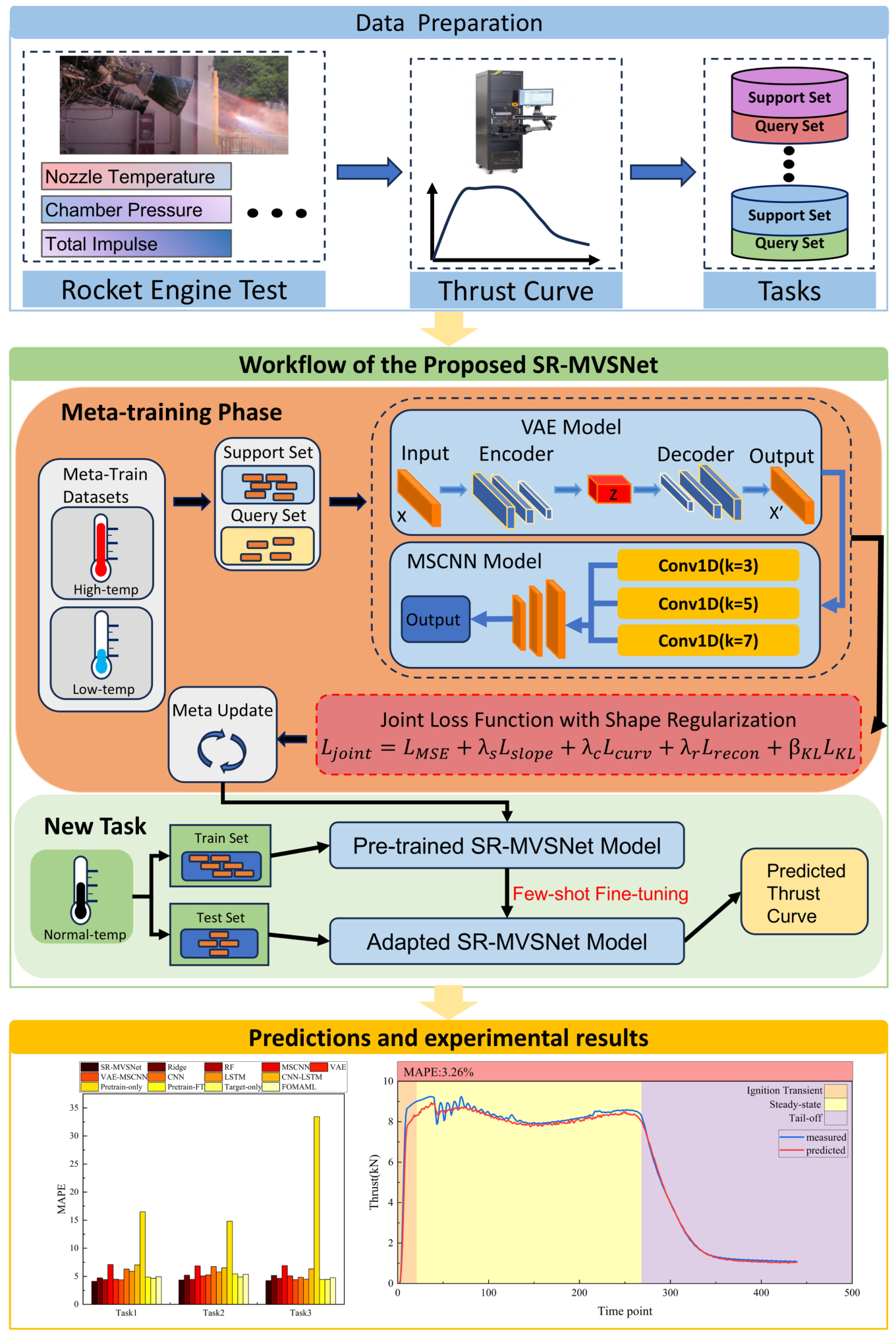
The comprehensive implementation workflow of the proposed solid rocket motor thrust prediction framework is illustrated in Figure 4. The procedure comprises three primary stages:

Step 1:

Each data record pairs nine static input parameters with a measured thrust curve. The source domains and the fixed target support/test partition are identified before normalization. Min–Max statistics are fitted using only the source-domain records of the current transfer task and are kept fixed when transforming target-domain data.

Step 2:

Meta-training tasks are sampled within each selected source domain. The default task contains six support samples for inner-loop adaptation and four query samples for the outer-loop update. The source-task losses are used to learn a shared initialization.

Step 3:

The meta-trained model is adapted using the 21 ambient-temperature support samples in the main configuration, then evaluated on the five held-out target test samples. The few-shot experiments use smaller subsets of the same support pool while retaining the same test set. The held-out test set is reserved for final evaluation.

4. Experimental Setup

4.1. Dataset Description and Task Construction

The experimental data were obtained from confidential ground static firing tests involving a single physical solid rocket motor test article. The identity of the testing organization is withheld under the applicable confidentiality requirements. Each data record corresponds to one firing test and contains one measured thrust curve. To evaluate the generalization capability of the proposed model under few-shot scenarios across varying operating environments, the dataset encompasses three distinct initial temperature conditions: high, low, and ambient. The nine input variables, in their recorded order, are propellant mass, web thickness coefficient, propellant density, ambient temperature, ambient pressure, burning-rate coefficient, pressure exponent, burning-area variation coefficient, and nozzle throat area. Each input vector is paired with the measured thrust curve obtained in the corresponding firing test.

The high-, low-, and ambient-temperature groups correspond to pre-ignition environmental conditions of 50 °C, −40 °C, and 20 °C, respectively. Initial propellant temperature can affect burning rate and thereby alter gas generation, chamber pressure, and thrust evolution. The recorded ambient temperature describes the thermal operating condition; it is not a measurement of the internal propellant temperature distribution. Ambient pressure is also included among the nine inputs because external pressure affects nozzle pressure thrust. The present transfer tasks are organized by temperature, and the relative sensitivities to temperature and ambient pressure are not separately evaluated.

Table 1. Physical input parameters used in SR-MVSNet.

No.	Physical Parameter	Symbol	Unit	Definition/Physical Meaning
1	Propellant mass	$m_p$	kg	Total mass of the solid propellant loaded in the motor, representing the overall propellant scale and available mass for thrust generation.
2	Web thickness coefficient	$W_f$	Dimensionless	Defined as $W_f=w/R_g$, where w is the effective propellant web thickness and $R_g$ is the outer radius of the propellant grain. It characterizes the relative burning thickness of the grain independent of the absolute motor size.
3	Propellant density	${\rho }_p$	$\mathrm{kg}·{\mathrm{m}}^{-3}$	Density of the solid propellant, which determines the propellant mass consumed per unit burning volume and directly affects the gas-generation mass flow rate.
4	Ambient temperature	$T_a$	K	Ambient temperature before motor ignition. It characterizes the initial thermal operating condition of the motor and may influence the combustion behavior of the propellant.
5	Ambient pressure	$P_a$	Pa	External static pressure surrounding the motor before and during operation, which affects the pressure-thrust component of the nozzle.
6	Burning-rate coefficient	a	$\mathrm{mm}·{\mathrm{s}}^{-1}$$·{\mathrm{MPa}}^{-n}$	Empirical coefficient in the pressure-dependent burning-rate law $r=a{P}_c^n$, where r is the propellant burning rate and $P_c$ is the chamber pressure.
7	Pressure exponent	n	Dimensionless	Pressure sensitivity exponent in $r=a{P}_c^n$, describing the nonlinear sensitivity of the propellant burning rate to chamber pressure.
8	Burning-area variation coefficient	$C_{Ab}$	Dimensionless	Defined as $C_{Ab}=A_{b,f}/A_{b,0}$, where $A_{b,0}$ and $A_{b,f}$ denote the burning surface areas at the beginning and end of the main burning stage, respectively. $C_{Ab}>1$, $C_{Ab}\approx 1$, and $C_{Ab}<1$ correspond to progressive, approximately neutral, and regressive burning characteristics, respectively.
9	Nozzle throat area	$A_t$	${\mathrm{m}}^2$	Minimum flow area of the nozzle, which governs the discharge capacity of the combustion gas and strongly influences chamber pressure and thrust level.

Note: The propellant burning rate is described using the empirical pressure law $r=a{P}_c^n$, where r is expressed in $\mathrm{mm}·{\mathrm{s}}^{-1}$ and $P_c$ in MPa. Accordingly, the numerical value and unit of a depend on the adopted pressure and burning-rate units. Input parameters are normalized using statistics calculated only from the source-domain meta-training records selected for each transfer configuration.

summarizes the symbols, units, and physical meanings of the nine input parameters.

The input features comprise nine static parameters, and the prediction target is a 440-point thrust sequence. The original thrust measurements were acquired during ground static firing tests at approximately 14 kHz, with each raw record containing more than one million sampling points. A window was first extracted from the thrust record using the index range [51,100, 400,000).

Table 2. Segment-wise downsampling of the thrust records.

Segment	Index Range Within Window	Points Before Sampling	Sampling Stride	Retained Points
1	[0, 1000)	1000	10	100
2	[1000, 50,000)	49,000	200	245
3	[50,000, 347,900)	297,900	3150	95
Total	[0, 347,900)	347,900	—	440

Note: All index ranges use zero-based indexing with an inclusive lower bound and an exclusive upper bound. The segment ranges are relative to the extracted window. Sampling starts from the first point of each segment, and a stride of k retains every kth point. The final 1000 points of the extracted window are excluded.

summarizes the three-segment downsampling scheme applied within this window. The sampled segments were concatenated in chronological order to form the 440-point target sequence.

The segment-specific strides produce nonuniform spacing in physical time; the sampling intervals are determined by these strides and the original acquisition rate.

The VAE reconstructs the normalized input parameters, while the MSCNN predicts the normalized thrust target. Min–Max normalization is fitted separately for each transfer configuration using only its source-domain meta-training records. Statistics are computed independently for each of the nine input coordinates and each of the 440 thrust-output positions. For a scalar coordinate v, the transformation is

$$\begin{array}{cc}\hfill \tilde{v}& ={\displaystyle \frac{v-v_{min,s}}{s_v}},{\Delta }_v=v_{max,s}-v_{min,s},\hfill \\ \hfill s_v& =\left\{\begin{array}{cc}1,\hfill & {\Delta }_v\le {10}^{-8},\hfill \\ {\Delta }_v+{10}^{-8},\hfill & {\Delta }_v>{10}^{-8}.\hfill \end{array}\right.\hfill \end{array}$$

(10)

Here, $v_{min,s}$ and $v_{max,s}$ are the minimum and maximum of that coordinate over the selected source records. The scale is set to one for coordinates whose source range is at most ${10}^{-8}$. The fixed source-derived transformation is applied to both the target support set and the target test set, retaining transformed values outside $[0,1]$. Predicted thrust is returned to the original label scale using the same source-derived output statistics before error metrics are calculated. The dataset contains 84 high-temperature firing tests, 73 low-temperature firing tests, and 26 ambient-temperature firing tests, for a total of 183 tests. Each firing test contributes one measured thrust curve and is treated as one sample in the dataset. Task 1 uses the combined high- and low-temperature samples for source-domain meta-training. Tasks 2 and 3 use only the high-temperature and low-temperature source samples, respectively. For all three transfer configurations, the existing ambient-temperature partition contains 21 target support samples for adaptation and five held-out target test samples for evaluation. This target partition is fixed throughout the experiments, with the held-out test set reserved exclusively for final evaluation after training and model selection.

Within each selected source domain, sample indices are randomly permuted once per run to construct the meta-training tasks. In the default configuration, each task contains $K=6$ support samples and $M=4$ query samples. Each task has disjoint support and query sets. Support blocks are disjoint across source tasks, while a source query sample may also appear in another source task’s support set.

4.2. Experimental Environment and Parameter Settings

4.2.1. Network Architecture Parameters

The proposed SR-MVSNet framework comprises a variational feature extraction module and a multi-scale convolutional regression module, with its detailed structural hyperparameters summarized in

Table 3. Parameter settings of the VAE module.

Parameter Name	Values	Parameter Name	Values
Input dimension	9	Output dimension	9
Latent dimension	80	Hidden dimension	160
Activation function	GELU	Dropout rate	0.15
Encoder linear layers	3	Decoder linear layers	3

. The Variational Autoencoder employs a symmetrical, fully connected architecture. To extract robust latent features from a restricted sample size, both the encoder and decoder utilize three dense layers. The hidden dimension is 160 and the latent dimension is 80; the encoder input and decoder output each contain nine parameters. Furthermore, a Dropout layer with a rate of 0.15 is incorporated following Gaussian Error Linear Unit (GELU) [42] activation. This regularization strategy mitigates the risk of overfitting to the limited support set during the inner-loop adaptation phase of the meta-learning process.

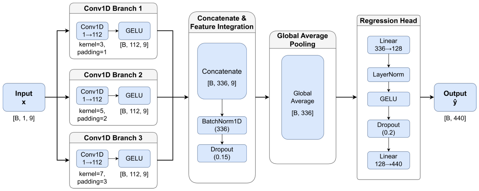
Figure 5 shows the computational workflow of the MSCNN module. The module receives the nine reconstructed parameters from the VAE as a tensor of shape $[B,1,9]$, where B denotes the number of records in the current batch, 1 denotes the input channel count, and 9 denotes the number of reconstructed parameters. The last dimension follows the fixed order of the nine static input features. Three parallel one-dimensional convolutional branches process this feature vector using different kernel sizes.

Each branch expands the channel dimension from 1 to 112, thereby enriching the feature representation capacity. The feature maps from these three branches are subsequently concatenated along the channel axis, yielding a fused representation of size [B, 336, 9]. This fused tensor is then regularized via Batch Normalization (BatchNorm) and Dropout layers. A Global Average Pooling (GAP) operation is employed to aggregate the sequence dimension, compressing the tensor into a global feature vector of [B, 336]. Finally, these features are projected into a 128-dimensional hidden space, processed through Layer Normalization (LayerNorm) and a GELU activation function, before a final linear mapping layer outputs the 440-dimensional predicted thrust profile.

4.2.2. Training Hyperparameters

The overall training procedure is partitioned into a meta-learning phase and a subsequent target fine-tuning phase. During the meta-learning phase, the inner loop employs the Stochastic Gradient Descent (SGD) optimizer [43] to perform rapid gradient adaptation on the support set. The automatic differentiation engine computes the gradients required for the inner-loop adaptation and outer-loop meta-parameter updates. In the outer loop, the Adam optimizer is utilized to update the global meta-parameters. Subsequently, during the fine-tuning phase, the AdamW optimizer is employed to further refine the model weights, thereby enhancing the final predictive accuracy [44,45]. The specific training hyperparameters are detailed in

Table 4. Training hyperparameter settings.

Category	Parameter	Value
Meta-learning	Meta Epochs	1800
	Meta LR ($\beta$)	0.005
	Inner Steps	5
	Inner LR ($\alpha$)	0.004
Fine-tuning	FT Epochs	1200
	FT LR	0.0006
Loss Weights	${\beta }_{\mathrm{KL}}$	0.002
	${\lambda }_r$	0.1
	${\lambda }_s$	0.5
	${\lambda }_c$	0.05

LR: learning rate; FT: fine-tuning.

.

4.3. Evaluation Indicators

This study evaluates predictive performance using mean squared error (MSE), root mean squared error (RMSE), mean absolute error (MAE), and mean absolute percentage error (MAPE).

MSE and RMSE give greater weight to larger deviations, whereas MAE measures the mean magnitude of pointwise errors. MAPE expresses absolute prediction errors as percentages of the corresponding measured thrust magnitudes. The metrics are evaluated on the original thrust scale after inverse normalization using the source-domain output statistics.

$$\mathrm{MSE}={\displaystyle \frac{1}{N}}{\displaystyle \sum _{i=1}^N}{({\widehat{y}}_i-y_i)}^2$$

(11)

$$\mathrm{RMSE}=\sqrt{{\displaystyle \frac{1}{N}}{\displaystyle \sum _{i=1}^N}{({\widehat{y}}_i-y_i)}^2}$$

(12)

$$\mathrm{MAE}={\displaystyle \frac{1}{N}}{\displaystyle \sum _{i=1}^N}|{\widehat{y}}_i-y_i|$$

(13)

$$\mathrm{MAPE}={\displaystyle \frac{100\%}{N}}{\displaystyle \sum _{i=1}^N}{\displaystyle \frac{|{\widehat{y}}_i-y_i|}{\left|y_i\right|}}$$

(14)

Here, $y_i$ and ${\widehat{y}}_i$ denote measured and predicted thrust, respectively, and N is the number of scalar thrust values evaluated. An individual curve contains $N=440$ points; the overall evaluation pools the five held-out curves, giving $N=2200$. Segment-wise metrics use the corresponding subset of points. All evaluated reference values are nonzero, so MAPE is calculated directly using their absolute magnitudes. Small-magnitude reference values receive greater relative weight. MSE has squared thrust units, RMSE and MAE have thrust units, and MAPE is expressed as a percentage.

Each configuration was evaluated using five runs with random seeds 42–46 and the same five held-out target test records. The reported mean and sample standard deviation are calculated from the five per-run metric values. For a metric m, they are defined as

$$\overline{m}={\displaystyle \frac{1}{5}}{\displaystyle \sum _{r=1}^5}{m}_r,s_m=\sqrt{{\displaystyle \frac{1}{4}}{\sum }_{r=1}^5{(m_r-\overline{m})}^2}.$$

(15)

The sample standard deviations describe variation across runs on the fixed test set. Each metric is computed within each run before aggregation; in particular, mean RMSE is the mean of the five run-level RMSE values. Approximate 95% confidence intervals for the mean run-level metrics are reported in Appendix A.

5. Experimental Results and Analysis

The evaluation uses ground static firing measurements at initial temperatures of −40 °C, 20 °C, and 50 °C. The measurements were obtained in the confidential firing-test program described in Section 4.1 and were not extracted from a public database or published reference. The identity of the testing organization cannot be disclosed. Each firing test produced one measured thrust curve. The tests used a horizontal thrust stand equipped with load cells and a dynamic data acquisition system operating at approximately 14 kHz. The measurements were processed into 440-point reference curves as described in Section 4.1. In the prediction comparisons, Measured denotes the experimentally acquired reference curve and Predicted denotes the model output. Curve positions refer to the retained sample indices, whose spacing in physical time is nonuniform.

All results below use source-only normalization and the MAPE defined in Section 4.3. Tables report the mean ± sample standard deviation across five runs. Task 1, which combines the high- and low-temperature source records, is the reference setting for the overall, segment-wise, ablation, allocation, and few-shot analyses.

5.1. Overall Assessment

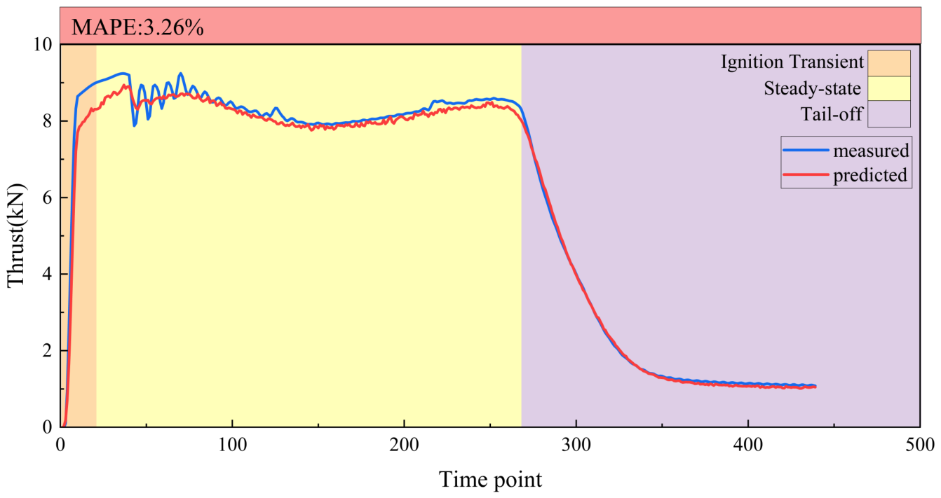
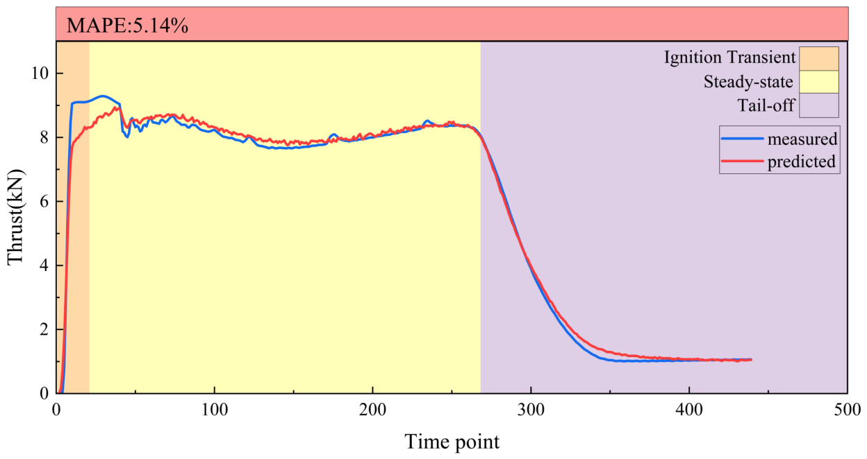
Figure 6 and Figure 7 compare the measured and predicted curves for test records 3 and 1, respectively, in the Task 1 run with seed 42. These records have the lowest and highest full-curve MAPE among the five test records in that run. The example selection is confined to this run, while the aggregate results use all five runs.

For record 3, MAPE is 3.26%, RMSE is 0.25386, and MAE is 0.16016. For record 1, the corresponding values are 5.14%, 0.26677, and 0.17033. Thus, a difference in relative error can coexist with similar absolute errors. The Task 1 aggregate MSE, RMSE, and MAE are 0.03034, 0.17411, and 0.11895, respectively; the full-curve MAPE is 4.11% (

Table 5. Task 1 full-curve and segment-wise errors.

Range	MSE	RMSE	MAE	MAPE (%)
Full curve	$0.03034\pm 0.00199$	$0.17411\pm 0.00572$	$0.11895\pm 0.00446$	$4.11\pm 0.11$
Ignition	$0.08000\pm 0.01126$	$0.28228\pm 0.01994$	$0.20000\pm 0.01413$	$31.92\pm 2.25$
Steady-state	$0.02680\pm 0.00322$	$0.16347\pm 0.00985$	$0.12603\pm 0.00759$	$1.71\pm 0.10$
Tail-off	$0.02954\pm 0.00268$	$0.17173\pm 0.00781$	$0.10051\pm 0.00457$	$4.22\pm 0.19$

). The individual-record results in Section 5.6 provide a five-run view of the sample-level variation.

SR-MVSNet maps design and operating parameters to complete thrust histories, providing a unified description of ignition build-up, sustained thrust, and tail-off. This whole-curve output supports comparisons of thrust level and profile shape across test records, with each operating phase available for separate assessment. Adaptation with the available target support records makes this representation useful for assessing the target condition when measurements are limited.

5.2. Key Feature Evaluation

The 440-point sequence is evaluated over three index ranges: ignition, $[0,20)$; steady-state combustion, $[20,260)$; and tail-off, $[260,440)$. The ranges use zero-based indexing, with an inclusive lower bound and an exclusive upper bound. They contain 20, 240, and 180 retained points per curve, respectively. These evaluation ranges are distinct from the three segments used for downsampling in Section 4.1.

Table 5 reports errors pooled across the same five test records within each range. This phase-resolved assessment connects prediction performance with distinct aspects of motor operation: thrust-load build-up during ignition, sustained thrust delivery during steady-state combustion, and residual thrust decay during tail-off. It therefore provides a more detailed basis for assessing the predicted motor response than a single full-profile error metric. Metrics weight each retained point equally rather than weighting by the nonuniform physical-time intervals.

5.2.1. Ignition Transient

The ignition range has the largest absolute errors, with a mean RMSE of 0.28228 and MAE of 0.20000. Its MAPE is 31.92%, compared with 4.11% over the full curve. Reporting absolute errors alongside MAPE distinguishes the magnitude of ignition-phase deviations from the relative weighting introduced by small measured thrust values.

A delayed or smoothed ignition rise can shift the predicted onset of loading and attenuate the estimated thrust-rise rate. These discrepancies matter when a predicted curve is used as an input to a structural-response analysis. The present phase-wise errors quantify thrust agreement; assessment of transient structural loading additionally requires resolved physical-time histories and a structural model.

5.2.2. Steady-State

During steady-state combustion, mean RMSE is 0.16347, MAE is 0.12603, and MAPE is $1.71\%\pm 0.10\%$ (mean ± sample standard deviation). This range has the lowest relative error of the three phases. The agreement in the sustained thrust supports comparison of the main combustion responses across test records. Combined with the physical timestamps of the retained points, the predicted thrust history can also provide an input for estimating the steady-state contribution to total impulse.

5.2.3. Tail-Off

The tail-off range has mean RMSE of 0.17173, MAE of 0.10051, and MAPE of 4.22%. Its absolute errors are lower than those of the ignition range. Compared with steady-state combustion, it has a higher RMSE and MAPE but lower MAE. Reporting both measures distinguishes the magnitude of residual thrust deviations from their size relative to the measured thrust.

5.3. Comparison and Ablation Experiments

5.3.1. Comparison of Multiple Models

SR-MVSNet is evaluated against 12 comparison configurations: Ridge, Random Forest (RF), MSCNN, VAE, VAE-MSCNN, CNN, LSTM, CNN-LSTM, source pretraining alone (Pretrain-only), pretraining followed by target fine-tuning (Pretrain-FT), target-only training (Target-only), and the first-order MAML configuration trained with MSE (FOMAML-MSE). Task 1 uses the combined high- and low-temperature source domains, Task 2 uses the high-temperature source domain, and Task 3 uses the low-temperature source domain. All three tasks evaluate the same ambient-temperature target test records. Task 1 evaluates interpolation between source temperatures; Tasks 2 and 3 evaluate transfer from a single source temperature with target support data available for adaptation.

Table 6. Full-curve errors across models in Task 1.

Model	MSE	RMSE	MAE	MAPE (%)
SR-MVSNet	$0.03034\pm 0.00199$	$0.17411\pm 0.00572$	$0.11895\pm 0.00446$	$4.11\pm 0.11$
Ridge	$0.04478\pm 0.00000$	$0.21162\pm 0.00000$	$0.13320\pm 0.00000$	$4.72\pm 0.00$
RF	$0.08463\pm 0.01253$	$0.29028\pm 0.02151$	$0.13748\pm 0.00412$	$4.42\pm 0.07$
MSCNN	$0.19506\pm 0.05362$	$0.43867\pm 0.05732$	$0.21533\pm 0.02306$	$7.10\pm 0.50$
VAE	$0.04393\pm 0.00136$	$0.20958\pm 0.00327$	$0.13142\pm 0.00132$	$4.48\pm 0.03$
VAE-MSCNN	$0.04083\pm 0.00094$	$0.20206\pm 0.00232$	$0.13121\pm 0.00322$	$4.39\pm 0.08$
CNN	$0.14542\pm 0.03035$	$0.37960\pm 0.04061$	$0.20938\pm 0.02296$	$6.29\pm 0.78$
LSTM	$0.15156\pm 0.06338$	$0.38241\pm 0.08152$	$0.18336\pm 0.03094$	$5.89\pm 0.59$
CNN-LSTM	$0.21471\pm 0.08163$	$0.45604\pm 0.09171$	$0.19874\pm 0.02055$	$7.03\pm 0.37$
Pretrain-only	$0.83089\pm 0.21566$	$0.90581\pm 0.11408$	$0.72226\pm 0.08192$	$16.49\pm 2.22$
Pretrain-FT	$0.04089\pm 0.00078$	$0.20221\pm 0.00193$	$0.13030\pm 0.00374$	$4.87\pm 0.09$
Target-only	$0.04548\pm 0.00521$	$0.21298\pm 0.01218$	$0.13583\pm 0.00457$	$4.66\pm 0.17$
FOMAML	$0.07008\pm 0.03213$	$0.25951\pm 0.05847$	$0.15266\pm 0.02226$	$4.94\pm 0.23$

,

Table 7. Full-curve errors across models in Task 2.

Model	MSE	RMSE	MAE	MAPE (%)
SR-MVSNet	$0.07298\pm 0.02452$	$0.26705\pm 0.04561$	$0.16177\pm 0.01648$	$4.35\pm 0.39$
Ridge	$0.05318\pm 0.00000$	$0.23061\pm 0.00000$	$0.14246\pm 0.00000$	$5.21\pm 0.00$
RF	$0.07829\pm 0.00831$	$0.27949\pm 0.01492$	$0.13419\pm 0.00209$	$4.46\pm 0.07$
MSCNN	$0.09851\pm 0.01218$	$0.31337\pm 0.01960$	$0.18512\pm 0.01242$	$6.85\pm 0.27$
VAE	$0.05183\pm 0.00254$	$0.22761\pm 0.00553$	$0.14927\pm 0.00783$	$5.08\pm 0.15$
VAE-MSCNN	$0.12059\pm 0.06707$	$0.33631\pm 0.09672$	$0.16795\pm 0.01346$	$5.25\pm 0.16$
CNN	$0.09840\pm 0.01187$	$0.31325\pm 0.01859$	$0.18046\pm 0.01607$	$6.73\pm 0.31$
LSTM	$0.30128\pm 0.09192$	$0.54349\pm 0.08587$	$0.19424\pm 0.01832$	$5.78\pm 0.75$
CNN-LSTM	$0.13899\pm 0.04498$	$0.36842\pm 0.06382$	$0.18269\pm 0.01488$	$6.51\pm 0.58$
Pretrain-only	$0.67197\pm 0.01761$	$0.81968\pm 0.01082$	$0.66605\pm 0.01310$	$14.82\pm 0.19$
Pretrain-FT	$0.15673\pm 0.09183$	$0.38051\pm 0.12216$	$0.17785\pm 0.01530$	$5.43\pm 0.15$
Target-only	$0.05651\pm 0.00889$	$0.23714\pm 0.01857$	$0.15244\pm 0.00991$	$4.88\pm 0.26$
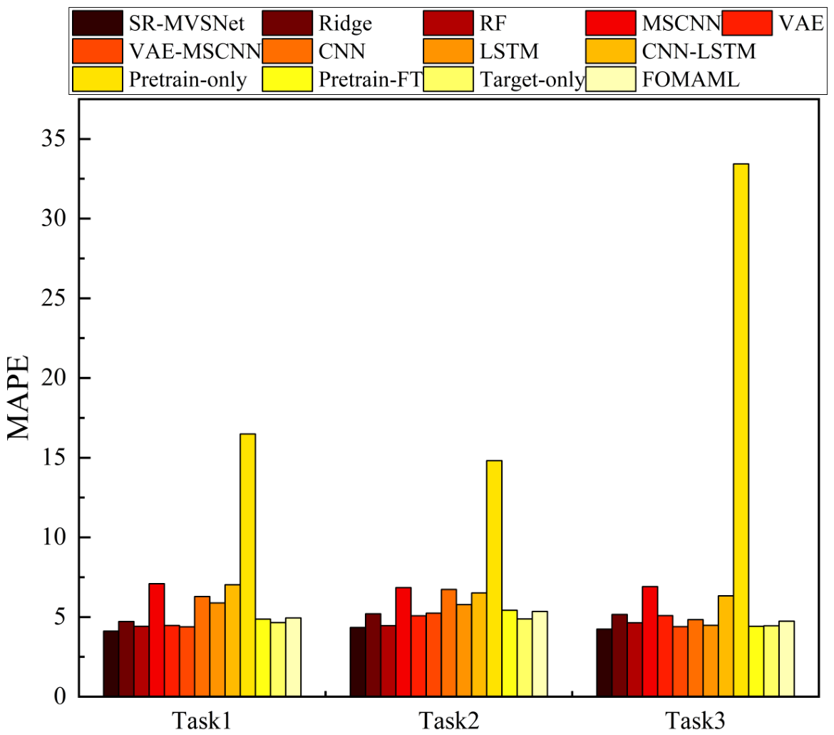
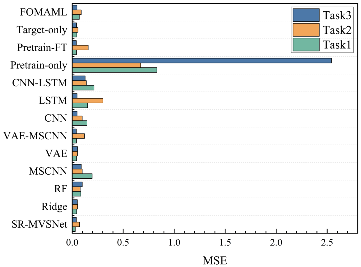
FOMAML	$0.08885\pm 0.06159$	$0.28649\pm 0.09200$	$0.15792\pm 0.01843$	$5.36\pm 0.40$

and

Table 8. Full-curve errors across models in Task 3.

Model	MSE	RMSE	MAE	MAPE (%)
SR-MVSNet	$0.03996\pm 0.00138$	$0.19987\pm 0.00344$	$0.13261\pm 0.00686$	$4.24\pm 0.13$
Ridge	$0.05021\pm 0.00000$	$0.22408\pm 0.00000$	$0.13635\pm 0.00000$	$5.17\pm 0.00$
RF	$0.09893\pm 0.01318$	$0.31394\pm 0.02156$	$0.14060\pm 0.00389$	$4.64\pm 0.12$
MSCNN	$0.08879\pm 0.01247$	$0.29736\pm 0.02127$	$0.18413\pm 0.01502$	$6.91\pm 0.15$
VAE	$0.05288\pm 0.00181$	$0.22992\pm 0.00395$	$0.14196\pm 0.00700$	$5.09\pm 0.09$
VAE-MSCNN	$0.04034\pm 0.00068$	$0.20085\pm 0.00168$	$0.13069\pm 0.00236$	$4.40\pm 0.02$
CNN	$0.04809\pm 0.00557$	$0.21902\pm 0.01251$	$0.14078\pm 0.00621$	$4.84\pm 0.29$
LSTM	$0.04770\pm 0.00772$	$0.21785\pm 0.01743$	$0.13872\pm 0.01224$	$4.49\pm 0.12$
CNN-LSTM	$0.12714\pm 0.05491$	$0.34980\pm 0.07733$	$0.17235\pm 0.02389$	$6.33\pm 0.64$
Pretrain-only	$2.54194\pm 0.02064$	$1.59434\pm 0.00649$	$1.35821\pm 0.00852$	$33.44\pm 0.10$
Pretrain-FT	$0.04044\pm 0.00040$	$0.20109\pm 0.00099$	$0.13207\pm 0.00293$	$4.42\pm 0.06$
Target-only	$0.04209\pm 0.00212$	$0.20511\pm 0.00510$	$0.13826\pm 0.01016$	$4.45\pm 0.17$
FOMAML	$0.04676\pm 0.00455$	$0.21604\pm 0.01062$	$0.14818\pm 0.01675$	$4.74\pm 0.33$

show that model rankings depend on both the source configuration and the error metric. In Task 1, SR-MVSNet achieves the lowest mean MSE, at 0.03034, compared with 0.04083 for VAE-MSCNN and 0.04089 for Pretrain-FT. In Task 2, VAE and Ridge yield mean MSE values of 0.05183 and 0.05318, compared with 0.07298 for SR-MVSNet. In Task 3, SR-MVSNet has the lowest mean MSE among the evaluated configurations, at 0.03996, followed by VAE-MSCNN at 0.04034 and Pretrain-FT at 0.04044. These closely spaced means are reported together with their run variability.

SR-MVSNet obtains mean MAPE values of 4.11%, 4.35%, and 4.24% in Tasks 1–3, respectively, lower than the RF values of 4.42%, 4.46%, and 4.64%. Its mean MSE is also lower than that of RF in each task. Across the evaluated configurations, SR-MVSNet achieves the lowest mean MAPE in all three tasks, while the MSE rankings vary with the source configuration.

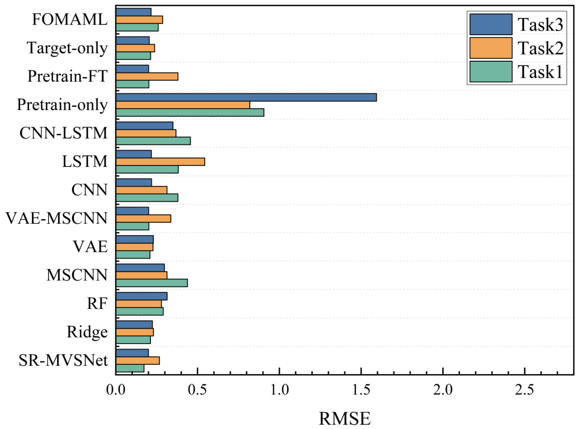
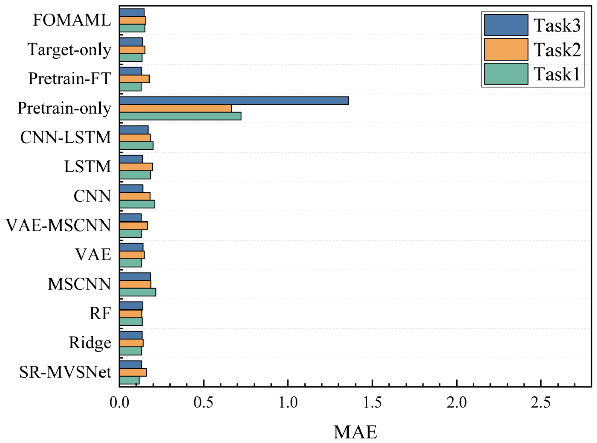
Figure 8 presents the MAPE results, and Figure 9, Figure 10 and Figure 11 summarize the absolute-error metrics across the three transfer tasks. Comparisons within each absolute-error metric complement the MAPE results. In Task 3, the mean MSE of SR-MVSNet is approximately 45.00% of the MSCNN value. The results identify source-dependent differences between the evaluated training configurations and support selecting a predictor according to the error measure relevant to the intended assessment.

The cross-temperature results show how source-temperature firing records can be reused for thrust prediction at the target ambient condition through adaptation with a limited support set. This reuse extends the assessment value of existing measurements to the evaluated target condition. The resulting thrust estimates support early performance comparisons and can help identify test cases that warrant more detailed experimental examination.

Task 1 is used for the following ablations so that each component comparison shares the same combined source domains, target partition, and set of random seeds.

5.3.2. VAE Assessment

Table 9. Task 1 errors with and without the VAE.

Configuration	MSE	RMSE	MAE	MAPE (%)
SR-MVSNet	$0.03034\pm 0.00199$	$0.17411\pm 0.00572$	$0.11895\pm 0.00446$	$4.11\pm 0.11$
No VAE	$0.26234\pm 0.06482$	$0.50929\pm 0.06087$	$0.34287\pm 0.04275$	$8.37\pm 0.52$

compares the complete framework with the no-VAE configuration. Removing the VAE increases mean MSE from 0.03034 to 0.26234 and MAPE from 4.11% to 8.37%; RMSE and MAE also increase. The consistently higher errors in this comparison support retaining the VAE feature-processing stage under Task 1.

The module maps the design and operating inputs to a probabilistic latent representation, with reconstruction and Kullback–Leibler (KL) regularization participating in training. For performance assessment with limited target data, the lower errors obtained with the VAE provide empirical support for using this feature-processing stage to improve thrust estimates.

5.3.3. Multi-Scale Feature Assessment

Table 10. Task 1 errors for multi-scale and single-scale feature processing.

Configuration	MSE	RMSE	MAE	MAPE (%)
SR-MVSNet	$0.03034\pm 0.00199$	$0.17411\pm 0.00572$	$0.11895\pm 0.00446$	$4.11\pm 0.11$
Single scale	$0.04234\pm 0.00250$	$0.20570\pm 0.00617$	$0.13747\pm 0.00479$	$4.58\pm 0.15$

compares the complete framework with the single-scale configuration. The complete framework achieves a lower mean MSE, RMSE, MAE, and MAPE, with an MSE of 0.03034 versus 0.04234 and MAPE of 4.11% versus 4.58% for the single-scale variant. The lower mean errors across all four metrics support multi-scale feature processing under Task 1. This experiment compares multi-scale and single-scale feature processing; the convolutional feature-processing stage is retained in both configurations.

Its parallel convolutional branches process different spans of the reconstructed input-feature vector before regression to the thrust curve. Combining these feature representations provides a means of mapping the static design and operating parameters to the complete thrust response.

5.3.4. Evaluation of Joint Loss Function

Table 11. Task 1 errors for the full objective and loss ablations.

Configuration	MSE	RMSE	MAE	MAPE (%)
SR-MVSNet	$0.03034\pm 0.00199$	$0.17411\pm 0.00572$	$0.11895\pm 0.00446$	$4.11\pm 0.11$
FOMAML-MSE	$0.07008\pm 0.03213$	$0.25951\pm 0.05847$	$0.15266\pm 0.02226$	$4.94\pm 0.23$
No shape	$0.04532\pm 0.00722$	$0.21235\pm 0.01668$	$0.13369\pm 0.00603$	$4.36\pm 0.29$
No slope	$0.04624\pm 0.00733$	$0.21451\pm 0.01669$	$0.13665\pm 0.00924$	$4.42\pm 0.17$
No curvature	$0.04396\pm 0.00275$	$0.20958\pm 0.00656$	$0.13452\pm 0.00544$	$4.41\pm 0.26$

reports the full objective, FOMAML-MSE, and the configurations recorded as no-shape, no-slope, and no-curvature. The saved settings identify zero slope and curvature weights for no-shape, a zero slope weight for no-slope, and a zero curvature weight for no-curvature. The MSE-only configuration disables all auxiliary losses, whereas the three shape-term ablations retain the other objective terms.

Relative to FOMAML-MSE, the complete framework reduces mean MSE from 0.07008 to 0.03034 and MAPE from 4.94% to 4.11%. The no-shape configuration obtains a mean MSE of 0.04532 and MAPE of 4.36%, and the no-slope and no-curvature configurations also have a higher mean MSE and MAPE than the complete framework. The complete framework achieves the lowest mean errors across all four metrics among the evaluated objectives. These results support retaining the joint loss and both shape-matching terms under Task 1.

Relation to physics-based models. CFD, quasi-steady-state (QSS) internal-ballistics models, and SR-MVSNet provide different forms of performance assessment. CFD resolves spatial flow variables for specified geometry, material models, and boundary conditions. QSS models estimate the evolution of chamber-averaged quantities using internal-ballistics relations under quasi-steady assumptions. SR-MVSNet learns a mapping from the recorded design and operating parameters to measured thrust curves, with target support records providing adaptation to the evaluated condition.

This data-driven mapping can complement physics-based analysis by providing record-based thrust estimates when measurements are limited. Geometry-resolved flow analysis and physically based examination of conditions beyond the observed data remain roles for mechanistic models. A matched CFD or QSS benchmark was not performed in this study, so quantitative comparisons of prediction error and computational cost remain open.

5.4. Analysis of Support Set and Query Set Allocation Strategies

This experiment varies the allocation within each ten-sample source-domain meta-training task: S5/Q5, S6/Q4, S7/Q3, and S8/Q2. The target partition remains fixed at 21 support records and five held-out test records.

Table 12. Task 1 errors under different source-task support/query allocations.

Configuration	MSE	RMSE	MAE	MAPE (%)
S5/Q5	$0.04235\pm 0.00300$	$0.20569\pm 0.00725$	$0.13052\pm 0.00270$	$4.36\pm 0.15$
S6/Q4	$0.03034\pm 0.00199$	$0.17411\pm 0.00572$	$0.11895\pm 0.00446$	$4.11\pm 0.11$
S7/Q3	$0.03462\pm 0.00160$	$0.18603\pm 0.00376$	$0.12390\pm 0.00355$	$4.24\pm 0.18$
S8/Q2	$0.04034\pm 0.01182$	$0.19953\pm 0.02568$	$0.12995\pm 0.01458$	$4.31\pm 0.22$

reports five-run results for each configuration; S6/Q4 is the default Task 1 configuration used in the preceding analyses.

The default S6/Q4 configuration has the lowest mean MSE, RMSE, MAE, and MAPE, at 0.03034, 0.17411, 0.11895, and 4.11%, respectively. Increasing the source support allocation beyond six samples does not further reduce the mean errors in these experiments. The allocation comparison concerns source-task construction, while the amount of target adaptation data is held constant.

5.5. Few-Shot Fit Experiment

This experiment varies the number of target support records available for adaptation, with $K=3$, 5, 10, and 20. The subsets are drawn from the existing pool of 21 ambient-temperature support records. For each seed, they are nested prefixes of one permutation of that pool. The same five held-out target test records are used throughout, and the source-task allocation remains S6/Q4.

Table 13. Task 1 errors at different target support sizes.

Configuration	MSE	RMSE	MAE	MAPE (%)
$K=3$	$0.08788\pm 0.02615$	$0.29375\pm 0.04465$	$0.20541\pm 0.02442$	$5.98\pm 1.29$
$K=5$	$0.06711\pm 0.02587$	$0.25564\pm 0.04695$	$0.16209\pm 0.02327$	$5.17\pm 0.58$
$K=10$	$0.06249\pm 0.02562$	$0.24638\pm 0.04731$	$0.16053\pm 0.02651$	$4.89\pm 0.45$
$K=20$	$0.03034\pm 0.00199$	$0.17411\pm 0.00572$	$0.11895\pm 0.00446$	$4.11\pm 0.11$

summarizes the results.

Mean MSE decreases from 0.08788 at $K=3$ to 0.06711, 0.06249, and 0.03034 at $K=5$, 10, and 20, respectively. Mean RMSE and MAE also decrease across these support sizes. MAPE changes from 5.98% to 5.17%, 4.89%, and 4.11%, decreasing across all four support sizes. Among the tested support sizes, $K=20$ gives the lowest mean values for all four metrics. The sample standard deviations across five runs show the accompanying variability, especially at the smaller support sizes.

The decrease in all four mean error metrics shows that SR-MVSNet can use additional target support records to improve thrust prediction over the tested range. The support size comparison provides an empirical reference for matching the available adaptation data to prediction accuracy, helping assess what can be achieved with an existing set of target-condition measurements. Selecting a cost-optimal testing strategy additionally requires experimental cost and decision-utility information.

5.6. Individual-Record Results

Table 14. Task 1 full-curve errors for individual held-out records.

Record	MSE	RMSE	MAE	MAPE (%)
1	$0.04028\pm 0.00637$	$0.20019\pm 0.01594$	$0.16107\pm 0.01283$	$4.96\pm 0.39$
2	$0.02854\pm 0.00451$	$0.16851\pm 0.01342$	$0.09685\pm 0.00771$	$4.19\pm 0.33$
3	$0.02810\pm 0.00444$	$0.16721\pm 0.01332$	$0.10044\pm 0.00800$	$2.78\pm 0.22$
4	$0.02402\pm 0.00380$	$0.15459\pm 0.01231$	$0.10351\pm 0.00824$	$4.37\pm 0.35$
5	$0.03076\pm 0.00486$	$0.17494\pm 0.01393$	$0.13288\pm 0.01058$	$4.25\pm 0.34$

reports Task 1 results separately for the five held-out records, using the same sample numbering as Figure 6 and Figure 7. Each cell summarizes five runs evaluated against a fixed reference curve. The record-level results retain the differences between test cases that are averaged in the pooled metrics.

5.7. Limitations

The evaluation uses a fixed set of five ambient-temperature test records obtained from five firing tests involving the single physical test article. The results characterize record-level transfer across the evaluated temperature conditions for this test article. The reported standard deviations characterize variation across random seeds on this fixed set; broader estimates of generalization require additional firing tests under other operating conditions. Task 1 evaluates temperature interpolation, and Tasks 2 and 3 evaluate single-source transfer with target adaptation data. Performance outside the evaluated temperature conditions remains to be established.

The nonuniformly sampled sequences place different densities of retained points in different physical-time intervals. The reported errors summarize agreement at those points, and MAPE is sensitive to the small-magnitude reference values in the ignition range. Predictive interval calibration, out-of-distribution detection performance, and reductions in the number and cost of firing tests are not evaluated here. The reported thrust-prediction errors also do not establish structural integrity or flight-safety margins.

6. Conclusions

This paper addresses the critical challenges of data scarcity and variable operating conditions in solid rocket motor thrust prediction by proposing a hybrid deep learning framework based on model-agnostic meta-learning (MAML). By combining variational feature processing, multi-scale convolutional prediction, and target-domain adaptation, the framework predicts complete thrust curves under limited sample conditions. The primary contributions and conclusions of this study are summarized as follows:

• The proposed SR-MVSNet framework supports few-shot thrust prediction when target-condition measurements are limited. Increasing the target support size from 3 to 20 reduces mean MSE from 0.08788 to 0.03034. Under the combined-source task, steady-state mean MAPE is 1.71%, and the VAE ablation supports retaining the variational feature-processing stage.
• SR-MVSNet transfers knowledge from the source-temperature records to the ambient-temperature target condition, achieving mean MSE values of 0.03034, 0.07298, and 0.03996 in Tasks 1–3, respectively. It obtains the lowest mean MSE among the evaluated models in Tasks 1 and 3. Under Task 1, the complete framework has lower mean errors than the single-scale and loss-ablation configurations. The framework combines source-data reuse with target adaptation to provide complete thrust estimates from limited target-condition measurements. These estimates support comparisons of ignition, sustained-thrust, and tail-off responses within the evaluated transfer settings.

Future research will investigate the model’s adaptability across a broader spectrum of extreme operational environments and expand its application to predict other critical internal ballistic parameters. Additionally, an attention mechanism will be investigated to enhance the model’s representation of ignition dynamics. Predictive uncertainty and out-of-distribution detection will also be evaluated using additional independent firing records.

References

1. Mahjub, A.; Mazlan, N.M.; Abdullah, M.Z.; Azam, Q. Design Optimization of Solid Rocket Propulsion: A Survey of Recent Advancements. J. Spacecr. Rocket. 2020, 57, 199–214. [Google Scholar] [CrossRef] [Scilit]
2. Wang, S.; Liu, F.; Chao, T.; Yang, M. Robust spline-line energy management guidance algorithm with multiple constraints and uncertainties for solid rocket ascending. Chin. J. Aeronaut. 2022, 35, 214–234. [Google Scholar] [CrossRef] [Scilit]
3. Sella, V.; Larkey, A.; Majumder, A.; Rao, A.; Abidi, Z.; Rasmont, N.; Randeo, A.; Liu, M.; Moore, A.K.; Lembeck, M.F. Development of a Nytrox-Paraffin Hybrid Rocket Engine. In Proceedings of the AIAA Propulsion and Energy 2020 Forum, Virtual, 24–28 August 2020. Paper AIAA 2020-3729. [Google Scholar]
4. Tola, C.; Nikbay, M. Internal Ballistic Modeling of a Solid Rocket Motor by Analytical Burnback Analysis. J. Spacecr. Rocket. 2020, 57, 116–126. [Google Scholar] [CrossRef] [Scilit]
5. Tizón, J.M. Burnback Analysis of Solid Propellant Rocket Motors. arXiv 2023, arXiv:2301.04559. [Google Scholar]
6. Yan, D.; Zhao, Z.; Song, A.; Li, F.; Ye, L.; Zhao, G.; Ma, S. Transient Characteristics of Fluidic Pintle Nozzle in a Solid Rocket Motor. Aerospace 2024, 11, 243. [Google Scholar] [CrossRef] [Scilit]
7. Manchiraju, V.N.M.; Dwivedi, V.K. Prediction of solid rocket motor performance characteristics using computational fluid dynamics and validation with experimental data. In Proceedings of the IOP Conference Series: Materials Science and Engineering; IOP Publishing: Bristol, UK, 2020; Volume 998, p. 012014. [Google Scholar]
8. Di Martino, G.D.; Carmicino, C.; Mungiguerra, S.; Savino, R. The Application of Computational Thermo-Fluid-Dynamics to the Simulation of Hybrid Rocket Internal Ballistics with Classical or Liquefying Fuels: A Review. Aerospace 2019, 6, 56. [Google Scholar] [CrossRef] [Scilit]
9. Takahashi, T.T. Development of Improved Empirical Take-Off Equations. Aerospace 2025, 12, 695. [Google Scholar] [CrossRef] [Scilit]
10. AbdelGawad, A.R.; Guozhu, L. A Numerical Simulation Study for A Dual Thrust Solid Propellant Rocket Motor Nozzle. J. Phys. Conf. Ser. 2022, 2235, 012010. [Google Scholar] [CrossRef] [Scilit]
11. Li, W.; He, Y.; Zhang, Y.; Liang, G. Design and Optimization of Modular Solid Rocket Grain Matching Multi-Thrust Performance Curve. Appl. Sci. 2025, 15, 6827. [Google Scholar] [CrossRef] [Scilit]
12. de Carvalho, D.J.R.G. Numerical analysis of the quasi-steady-state method for the unsteady modeling of the solid-fuel scramjet. Aerosp. Sci. Technol. 2025, 164, 110357. [Google Scholar] [CrossRef] [Scilit]
13. Memarzadeh, M.; Matthews, B.; Avrekh, I. Unsupervised Anomaly Detection in Flight Data Using Convolutional Variational Auto-Encoder. Aerospace 2020, 7, 115. [Google Scholar] [CrossRef] [Scilit]
14. Luo, X.J.; Oyedele, L.O. Forecasting building energy consumption: Adaptive long-short term memory neural networks driven by genetic algorithm. Adv. Eng. Inform. 2021, 50, 101357. [Google Scholar] [CrossRef] [Scilit]
15. Reddy, A.S.; Akashdeep, S.; Harshvardhan, R.; Kamath, S.S. Stacking Deep learning and Machine learning models for short-term energy consumption forecasting. Adv. Eng. Inform. 2022, 52, 101542. [Google Scholar] [CrossRef] [Scilit]
16. Waxenegger-Wilfing, G.; Dresia, K.; Deeken, J.; Oschwald, M. A Reinforcement Learning Approach for Transient Control of Liquid Rocket Engines. IEEE Trans. Aerosp. Electron. Syst. 2021, 57, 3328–3343. [Google Scholar] [CrossRef] [Scilit]
17. Yang, H.; Yu, P.; Lou, B.; Cui, Y.; Li, X. Deep learning-enabled turbulence model optimization of solid motor. Adv. Eng. Inform. 2025, 64, 103072. [Google Scholar] [CrossRef] [Scilit]
18. Yang, H.; Wang, X.; Zheng, S.; Xu, M.; Li, X. Prediction of Solid Rocket Motor Performance Based on Deep Learning and Ignition Experimental Data. IEEE Trans. Aerosp. Electron. Syst. 2024, 60, 6241–6255. [Google Scholar] [CrossRef] [Scilit]
19. Huang, R.; Huang, C.; Liu, Y.; Dai, G.; Kong, W. LSGCN: Long Short-Term Traffic Prediction with Graph Convolutional Networks. In Proceedings of the Twenty-Ninth International Joint Conference on Artificial Intelligence (IJCAI-20), Virtual, 7–15 January 2021; pp. 2355–2361. [Google Scholar]
20. Zhang, T.; Chen, J.; Li, F.; Zhang, K.; Lv, H.; He, S.; Xu, E. Intelligent fault diagnosis of machines with small & imbalanced data: A state-of-the-art review and possible extensions. ISA Trans. 2022, 119, 152–171. [Google Scholar] [CrossRef] [Scilit] [PubMed]
21. Fu, Y.; Hu, Y.; Hu, C.; Li, F.; Li, C. Erosion characteristics of molten aluminum droplets bouncing off solid walls in solid rocket motors. Acta Astronaut. 2022, 201, 431–444. [Google Scholar] [CrossRef] [Scilit]
22. Gamdha, D.; Unnikrishnakurup, S.; Rose, K.J.J.; Surekha, M.; Purushothaman, P.; Ghose, B.; Balasubramaniam, K. Automated Defect Recognition on X-ray Radiographs of Solid Propellant Using Deep Learning Based on Convolutional Neural Networks. J. Nondestruct. Eval. 2021, 40, 18. [Google Scholar] [CrossRef] [Scilit]
23. Zhang, W.; Li, X. Data privacy preserving federated transfer learning in machinery fault diagnostics using prior distributions. Struct. Health Monit. 2021, 20, 3326–3341. [Google Scholar] [CrossRef] [Scilit]
24. Zhang, W.; Li, X. Federated Transfer Learning for Intelligent Fault Diagnostics Using Deep Adversarial Networks with Data Privacy. IEEE/ASME Trans. Mechatron. 2021, 26, 2884–2894. [Google Scholar] [CrossRef] [Scilit]
25. Huisman, M.; van Rijn, J.N.; Plaat, A. A survey of deep meta-learning. Artif. Intell. Rev. 2021, 55, 1989–2041. [Google Scholar] [CrossRef] [Scilit]
26. Tian, Y.; Zhao, X.; Huang, W. Meta-learning approaches for learning-to-learn in deep learning: A survey. Neurocomputing 2022, 494, 203–223. [Google Scholar] [CrossRef] [Scilit]
27. Mu, M.; Jiang, H.; Wang, X.; Dong, Y. A task-oriented theil index-based meta-learning network with gradient calibration strategy for rotating machinery fault diagnosis with limited samples. Adv. Eng. Inform. 2024, 62, 102870. [Google Scholar] [CrossRef] [Scilit]
28. Jose, S.T.; Simeone, O. Information-Theoretic Generalization Bounds for Meta-Learning and Applications. Entropy 2021, 23, 126. [Google Scholar] [CrossRef] [Scilit] [PubMed]
29. Moon, J.; Noh, Y.; Jung, S.; Lee, J.; Hwang, E. Anomaly detection using a model-agnostic meta-learning-based variational auto-encoder for facility management. J. Build. Eng. 2023, 68, 106099. [Google Scholar] [CrossRef] [Scilit]
30. Cinelli, L.P.; Marins, M.A.; da Silva, E.A.B.; Netto, S.L. Variational Methods for Machine Learning with Applications to Deep Networks; Springer: Cham, Switzerland, 2021. [Google Scholar]
31. Lee, D.B.; Min, D.; Lee, S.; Hwang, S.J. META-GMVAE: Mixture of Gaussian VAEs for Unsupervised Meta-Learning. In Proceedings of the International Conference on Learning Representations (ICLR 2021), Virtual, 3–7 May 2021. [Google Scholar]
32. Negri, M.; Fortuin, V.; Stühmer, J. Meta-learning richer priors for VAEs. In Proceedings of the 4th Symposium on Advances in Approximate Bayesian Inference, Virtual, 1 February 2022. [Google Scholar]
33. Berti, M.; Camilo da Silva, M.; Saccani, S.; Barbon Junior, S. Meta-learning approach for variational autoencoder hyperparameter tuning. J. Univers. Comput. Sci. 2025, 31, 668–682. [Google Scholar] [CrossRef] [Scilit]
34. Gordon, J.; Bronskill, J.; Nowozin, S.; Bauer, M.; Turner, R.E. Meta-learning probabilistic inference for prediction (VERSA). In Proceedings of the International Conference on Learning Representations (ICLR 2019), New Orleans, LA, USA, 6–9 May 2019. [Google Scholar]
35. Qi, G.; Yu, H. CMVAE: Causal Meta VAE for Unsupervised Meta-Learning. In Proceedings of the AAAI Conference on Artificial Intelligence, Washington, DC, USA, 7–14 February 2023; Volume 37, pp. 9480–9488. [Google Scholar]
36. Zhang, L.; Liu, Y.; Li, X. Meta Conditional VAE (MCVAE) for Deep Domain Generalization. Comput. Vis. Image Underst. 2021, 214, 103250. [Google Scholar]
37. Xu, W.; Liang, C.; Qiu, H.; Zhang, J.; Bao, W. Time-series clustering of high-speed photography based on Multi-channel Variational Autoencoder in a scramjet combustor. Appl. Therm. Eng. 2025, 270, 126164. [Google Scholar] [CrossRef] [Scilit]
38. Zapata Usandivaras, J.F.; Bauerheim, M.; Cuenot, B.; Urbano, A. Deep convolutional autoencoders for the time–space reconstruction of liquid rocket engine flames. Proc. Combust. Inst. 2024, 40, 105382. [Google Scholar] [CrossRef] [Scilit]
39. Zhu, X.; Cheng, Y.; Wu, J.; Hu, R.; Cui, X. Steady-state process fault detection for liquid rocket engines based on convolutional auto-encoder and one-class support vector machine. IEEE Access 2020, 8, 3144–3158. [Google Scholar] [CrossRef] [Scilit]
40. Lu, Y.; Sheng, B.; Li, Y.; Fu, G.; Jiang, S.; Jiang, Z. Adaptive Prediction of Compressor Cylinder Pressure Dynamics Using a Physics-Guided VAE-CNN State Space Model. Actuators 2025, 14, 535. [Google Scholar] [CrossRef] [Scilit]
41. Gong, Y.; Dang, W.; Li, P. An improved dynamical variational autoencoder framework for predicting aero-engine remaining useful life. J. Phys. Conf. Ser. 2024, 2816, 012007. [Google Scholar] [CrossRef] [Scilit]
42. Lee, M. Mathematical analysis and performance evaluation of the gelu activation function in deep learning. J. Math. 2023, 2023, 4229924. [Google Scholar] [CrossRef] [Scilit]
43. Johri, S.; Pratap, S.; Narayan, J.; Dwivedy, S.K. Sensory data classification for gait assessment using deep neural networks: A comparative study with SGD and Adam optimizer. In Proceedings of the 2024 IEEE International Conference on Interdisciplinary Approaches in Technology and Management for Social Innovation (IATMSI); IEEE: Piscataway, NJ, USA, 2024; Volume 2, pp. 1–6. [Google Scholar]
44. Reyad, M.; Sarhan, A.M.; Arafa, M. A modified Adam algorithm for deep neural network optimization. Neural Comput. Appl. 2023, 35, 17095–17112. [Google Scholar] [CrossRef] [Scilit]
45. Nabila, P.; Setiawan, E.B. Adam and adamw optimization algorithm application on bert model for hate speech detection on twitter. In Proceedings of the 2024 International Conference on Data Science and Its Applications (ICoDSA); IEEE: Piscataway, NJ, USA, 2024; pp. 346–351. [Google Scholar]
Figure 1. Schematic of a solid rocket motor. Colors distinguish the illustrated components, which are identified by labels and arrows.
Machines 14 01087 g001
Figure 2. Schematic illustration of model-agnostic meta-learning (MAML). Solid arrows show task-specific adaptation from the shared initialization θ toward θ 1 and θ 2 . Dashed lines indicate the correspondence between positions on the parameter axis and the loss curves. Yellow dots mark the shared initialization and its corresponding task-loss values.
Machines 14 01087 g002
Figure 3. VAE flowchart. Green denotes the encoder-side variables, red highlights the latent variable, and blue denotes the decoder and reconstructed output.
Machines 14 01087 g003
Figure 4. The comprehensive framework of SR-MVSNet. Top-panel labels illustrate test measurements, not the model input parameters.
Machines 14 01087 g004
Figure 5. MSCNN framework.
Machines 14 01087 g005
Figure 6. Measured and predicted thrust for test record 3 in Task 1, seed 42 (MAPE: 3.26%).
Machines 14 01087 g006
Figure 7. Measured and predicted thrust for test record 1 in Task 1, seed 42 (MAPE: 5.14%).
Machines 14 01087 g007
Figure 8. Full-curve MAPE across the three transfer tasks, averaged over five runs.
Machines 14 01087 g008
Figure 9. Mean MSE of the evaluated models across the three transfer tasks.
Machines 14 01087 g009
Figure 10. Mean RMSE of the evaluated models across the three transfer tasks.
Machines 14 01087 g010
Figure 11. Mean MAE of the evaluated models across the three transfer tasks.
Machines 14 01087 g011