Article

Analytical Grid Generation Method for CFD Simulations in Rolling-Piston Compressors

1
Jiangxi Province Key Laboratory of Light Alloy, School of Advanced Manufacturing, Nanchang University, Nanchang 330031, China
2
Institute of Energy Futures, Centre for Sustainable Energy Use in Food Chains, Brunel University London, Uxbridge, Middlesex UB8 3PH, UK
3
Centre for Compressor Technology, City St George’s, University of London, 10 Northampton Square, London EC1V 0HB, UK
*
Author to whom correspondence should be addressed.
These authors contributed equally to this work.
Machines 2026, 14(9), 1071; https://doi.org/10.3390/machines14091071
Submission received: 24 August 2026 / Revised: 15 September 2026 / Accepted: 16 September 2026 / Published: 18 September 2026
(This article belongs to the Special Issue High-Performance Compressor Design, Model Analysis and Application)

Abstract

The adoption of advanced three-dimensional Computational Fluid Dynamics (CFD) tools for the research and design of Rolling-Piston Compressors (RPCs) is severely constrained by the absence of efficient and reliable grid generation methods. To address this issue, this paper proposes a novel analytical grid generation method for the rotor fluid domain of RPCs based on the User-Defined Nodal Displacement (UDND). This method splits the rotor fluid domain into a vane region, a transition region and a core region according to geometric characteristics. The number of circumferential nodes in each region is adaptively determined based on the mapped lengths of the corresponding inner and outer boundaries, while node number normalization is employed to ensure precise control of the total number of nodes. Numerical tests demonstrate that the proposed method can generate O-type structured meshes with consistent topology and adaptive node allocation over the entire range of rotor rotation angles. The proposed method was verified by reference indicated pressure measurements on a small-scale RPC for refrigeration and air-conditioning applications, yielding mean absolute percentage errors of 6.30% and 7.42% and maximum pointwise relative errors of 12.70% and 20.99% at 80 and 120 Hz, respectively. The proposed method reduces the preprocessing time required for a typical CFD model of the machine from approximately 48 h to only 54 s. The improved quality and robustness of the generated mesh enhance the stability and convergence behavior of the solver, thereby enabling the use of advanced physical models, such as the real-gas equation of state, in the design and analysis of RPCs. This paper presents a rapid and reliable meshing strategy for CFD simulations of RPCs.

1. Introduction

As a typical rotary positive-displacement machine, the Rolling-Piston Compressor (RPC) is characterized by simple geometry, compactness, low manufacturing complexity and favorable performance [1]. Owing to these advantages, RPCs have been widely used in room air conditioners [2], household refrigerators [3] and commercial refrigeration systems [4]. Since their introduction into practical use in the 1960s, the global annual production of RPCs has reached approximately 200 million units, making them an indispensable core component of vapor-compression refrigeration systems [5].
Existing research on RPCs has predominantly relied on theoretical and experimental approaches. Theoretical studies are generally based on zero-dimensional or one-dimensional thermodynamic models, in which the thermodynamic state of the working fluid within the working chamber is treated either as spatially lumped or as varying only along a single direction [1]. Although these models are computationally efficient, they cannot resolve the spatial distribution of the internal flow field in sufficient detail and are therefore unable to faithfully capture the complex flow topology within the compression chamber, limiting further improvements in compressor design. Experimental studies, by contrast, commonly employ a black-box approach for overall compressor testing, whereby compressor performance is evaluated from the pressure, temperature and flow rate measured in the suction and discharge lines, together with the electrical input power [6]. To obtain transient information over the compression cycle, fast-response pressure sensors such as piezoresistive or piezoelectric transducers may be installed in the cylinder or end face to measure the variation in working-chamber pressure with rotor rotation angle and construct pressure–volume indicator diagrams. For example, Yang et al. [7] analyzed the indicated work and losses associated with the suction and discharge passages of a two-stage CO2 RPC, whereas Wu et al. [8] simultaneously measured the in-cylinder pressure and valve-reed displacement in an HC290 RPC to determine the discharge-valve opening timing. Although these methods resolve the temporal evolution of the compression cycle, the limited number and locations of measurement points prevent a complete reconstruction of the spatial distribution of the internal flow field. The Particle Image Velocimetry (PIV) approach provides planar velocity-field measurements and has been employed to visualize leakage flows in oil-free Roots blowers [9]. However, the PIV approach requires transparent optical access together with suitable laser-illumination and imaging paths. In RPCs, the enclosed metallic housing, narrow internal passages, and continuously evolving boundaries make reliable optical access difficult to achieve.
With the rapid advances in Computational Fluid Dynamics (CFD) and high-performance computing, three-dimensional CFD simulation has become an effective tool for resolving detailed internal flow in rotary positive-displacement machines, helping to predict and optimize the overall machine performance [10]. The same approach has also been applied to the analysis of other fluid power systems, including the energy losses and operation delays associated with the pipeline and fitting connections of aircraft hydraulic drives [11] and the hydrodynamic processes in the angular fitting connections of transport machine hydraulic drives [12]. In RPCs, the working cycle comprises suction, compression and discharge stages, during which the working-chamber volume varies periodically. Meanwhile, the eccentric rotation of the rotor is coupled with the reciprocating motion of the vane, while leakage clearances on the order of only a few micrometers exist between the rotor outer wall and cylinder inner wall and between the rotor outer wall and vane tip. Accurate simulation of these processes requires dynamic mesh techniques capable of handling complex moving boundaries and large deformations. The generation of high-quality meshes for the rotor fluid domain as it undergoes continuous motion and deformation therefore represents a key challenge in applying CFD to RPCs. In commercial CFD solvers based on the Finite Volume Method (FVM), commonly used dynamic mesh approaches include diffusion smoothing, spring smoothing, layering, key-frame remeshing and User-Defined Nodal Displacement (UDND). Among these, UDND adopts an external mesh generation strategy in which an independent set of nodal coordinates is generated in advance for each time step before the numerical solution [10]. This approach enables controlled displacement of the mesh nodes while preserving cell topology and connectivity, thereby intrinsically satisfying the space conservation law and avoiding the introduction of artificial source terms [13]. Moreover, since mesh quality can be optimized during grid generation using analytical functions, UDND offers distinct advantages in accommodating large deformations and maintaining adequate mesh resolution within narrow clearance regions.
The UDND method has been successfully applied to various types of rotary positive-displacement machines, including screw, scroll and sliding vane machines. Specifically, Kovacevic et al. [14] proposed an algebraic mesh generation strategy for screw compressors based on the UDND method. Using the rack-conjugate theory, the working domain of a twin-screw compressor was divided into two independent O-type mesh regions, while the internal mesh nodes were distributed using transfinite interpolation, followed by smoothing and orthogonalization. In addition, more complex rotor configurations, such as screw expanders with variable rotor pitch, have been investigated and shown to improve efficiency, especially in high-pressure applications [15]. The TwinMesh software developed by Hesse et al. is likewise based on the UDND principle and provides customized mesh generation solutions for screw and scroll compressors [16,17]. CFD simulations of sliding vane machines have been carried out using moving or deforming mesh techniques to account for the moving boundaries and large deformations [18,19,20]. Furthermore, analytical mesh generation methodologies based on the UDND principle have been established for sliding vane compressors, employing trigonometric parametric descriptions of the machine cross-section, algebraic control functions for the distribution of boundary nodes, stretching functions to control the mesh growth ratio between the leakage clearance regions and the core flow region, and transfinite interpolation combined with iterative orthogonalization and smoothing to generate the internal nodes, yielding O-type fully hexahedral meshes with seamless connectivity between the leakage clearances and the core working chambers [21]. Ye et al. [22] further developed and refined this UDND-based mesh generation methodology, substantially broadening its range of applicability. The improved method can accommodate a wider variety of sliding vane machine configurations, including multiple-acting chambers, non-circular stator profiles, offset vanes, and asymmetric vane tip profiles. In addition, numerical investigations have examined the influence of geometric parameters, such as the discharge port configuration, on the performance of sliding vane rotary compressors [23].
Although the UDND method has been successfully applied to screw, scroll and sliding vane machines, RPCs differ substantially from these machines in both geometric configuration and kinematic characteristics [1]. For example, in sliding vane machines, the vanes are mounted in radial slots of the rotor and rotate together with it. The working chambers are enclosed by the outer surface of the rotor, the inner surface of the cylinder (stator), the two side surfaces of the vanes, and the end plates. The principal leakage paths are the clearances between the vane tips and the cylinder inner surface and between the rotor outer surface and the cylinder inner surface. In contrast, in an RPC, the rotor undergoes eccentric rotation within the cylinder, while the vane is installed in a slot in the cylinder wall and remains in contact with the rotor outer surface throughout operation [24]. The working chambers are bounded by the cylinder inner surface, the rotor outer surface, the vane-side surfaces and the end plates, while the leakage paths include the clearance between the vane tips and rotor outer surface and that between the rotor outer surface and the cylinder inner surface [25]. Consequently, the two types of machines differ in the relative motion between the cylinder and rotor, the kinematic constraint imposed on the vane, and the spatial distribution of leakage clearances. Preliminary efforts have been made to address deforming mesh treatment for RPCs [26]. For instance, Farkas et al. [27] employed the coupled smoothing and local-remeshing approach available in ANSYS FLUENT 2022R1 to handle the dynamic mesh of an RPC. However, when very small clearances are involved, excessive cell distortion can trigger frequent remeshing, resulting in high computational cost and potentially introducing interpolation errors. Other studies have used built-in meshing templates in specialized positive-displacement machine simulation software, such as PumpLinx, for grid generation and numerical solution. Although such approaches are convenient to implement and generally provide good numerical robustness, the predefined mesh templates are relatively inflexible and have limited adaptability to non-standard geometries [28,29]. It should be noted that the aforementioned approaches rely largely on solver-embedded algorithms or software-specific meshing templates during grid generation. To date, a general and analytically controllable UDND mesh generation framework specifically tailored to the geometric and kinematic characteristics of RPCs has yet to be established.
To address the aforementioned limitations, this study proposes a novel analytical and split-based grid generation method for RPCs. Three-dimensional simulations were carried out on an RPC using the ANSYS FLUENT 2022R1 solver. To validate the simulation model with the analytical grid generation method, the simulated results were compared with the experimentally indicated pressure. Finally, the flow fields within the RPC under single-phase operating conditions were presented and analyzed.

2. Methodology

2.1. Methodology Overview

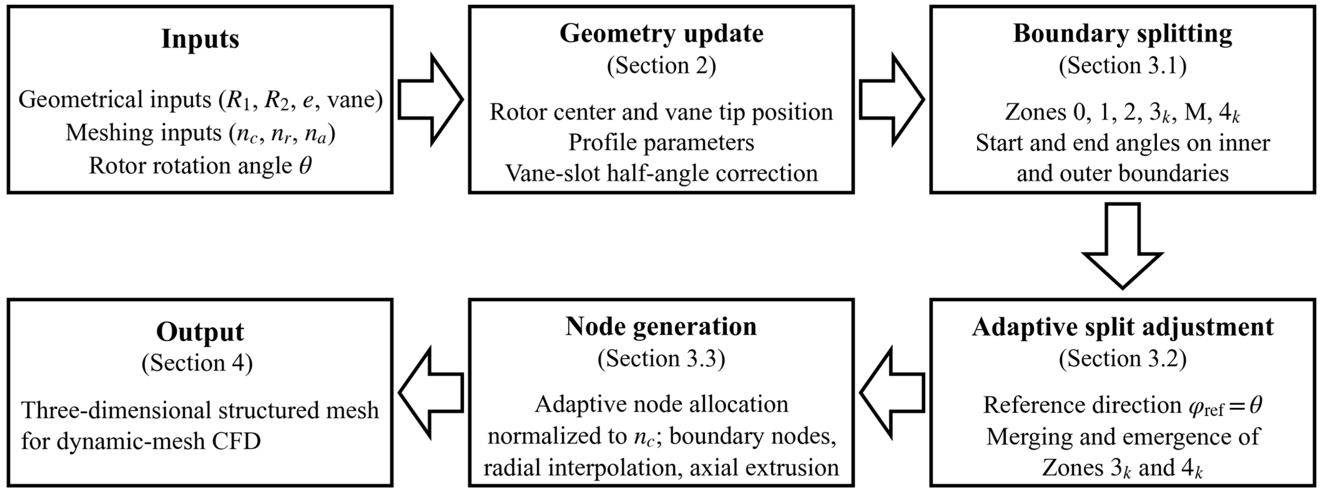
The methodology developed in this work analytically generates a structured, body-fitted mesh of the rotor fluid domain at an arbitrary rotor rotation angle θ . As outlined in Figure 1, the grid generation is driven by the rotor rotation angle θ and proceeds in four sequential steps: (i) Geometric updating—the positions of the rotor center and the center of the vane tip arc are determined from θ , and the parametric descriptions of the cylinder, rotor and vane profiles are updated accordingly (Section 2.3, Section 2.4 and Section 2.5). To alleviate local mesh degeneration caused by the rapid reduction in the vane protruding length as θ approaches 180°, a correction strategy for the half-angle of the vane slot opening is incorporated into the geometric-updating step (Section 2.6). (ii) Boundary splitting—the boundary of the two-dimensional cross-section is analytically split into a vane region ( Z o n e   1 ), transition regions ( Z o n e   0 , Z o n e   2 and Z o n e   M ) and core regions ( Z o n e   3 _ k and Z o n e   4 _ k ), with the start and end angles of each region determined on the inner and outer boundaries (Section 3.1); (iii) Adaptive split adjustment—a dynamic region-adjustment mechanism governed by a prescribed reference direction φ r e f = θ activates, merges or removes candidate subregions, keeping the split topology continuous and free of degenerate cells over the entire revolution (Section 3.2); and (iv) Node generation and three-dimensional construction—the circumferential node number of each region is adaptively assigned from the mapped lengths of its inner and outer boundaries under a normalization constraint on the total node number n c , after which boundary nodes, radial interior nodes and axial layers are generated to form the three-dimensional structured grid (Section 3.3). The resulting structured meshes provide the basis for the dynamic mesh CFD simulations presented in Section 4.

2.2. Geometric Features

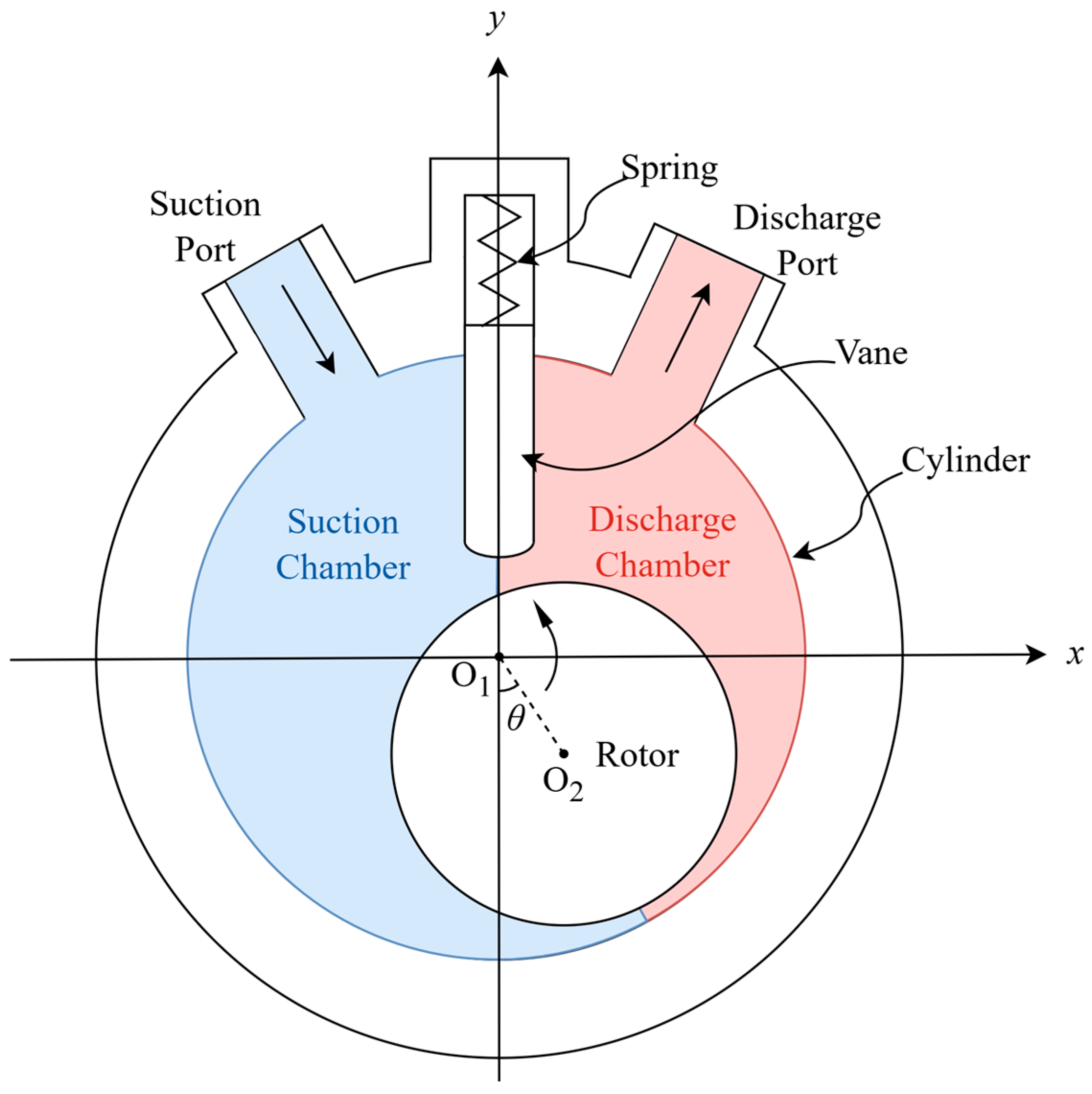
The core components of the RPC include the cylinder, rotor, vane, spring, suction port and discharge port, as shown in Figure 2. The cylinder is stationary and has a cylindrical inner wall. The rotor is a cylindrical body eccentrically installed inside the cylinder and rotates around the cylinder center. The vane reciprocates radially within a slot and toward the rotor outer surface. This configuration divides the crescent-shaped flow channel between the cylinder and the rotor into a suction chamber and a discharge chamber. As the rotor rotates, the volumes of the two chambers vary periodically, completing the suction, compression and discharge processes of the working fluid.
To establish the geometric basis for grid generation, a two-dimensional Cartesian coordinate system ( x , y ) fixed at the cylinder center is adopted, with the z axis along the compressor axis. Section 2.3, Section 2.4 and Section 2.5 provide the analytical descriptions of the cylinder, rotor and vane profiles respectively, together with the corresponding geometric parameters.
For an arbitrary rotor rotation angle θ , the grid generation procedure distributes n c circumferential nodes and n r radial node layers within the flow channel bounded by the cylinder inner wall (outer boundary) and the rotor outer wall (inner boundary) to form a two-dimensional structured face grid; this grid is then extruded uniformly in the axial direction into n a layers, giving a total node number of
n t = n c   n r   n a
where n t is the total number of nodes of the three-dimensional grid; n c is the total number of circumferential nodes; n r is the number of radial node layers; and n a is the number of axial node layers.

2.3. Cylinder Profile

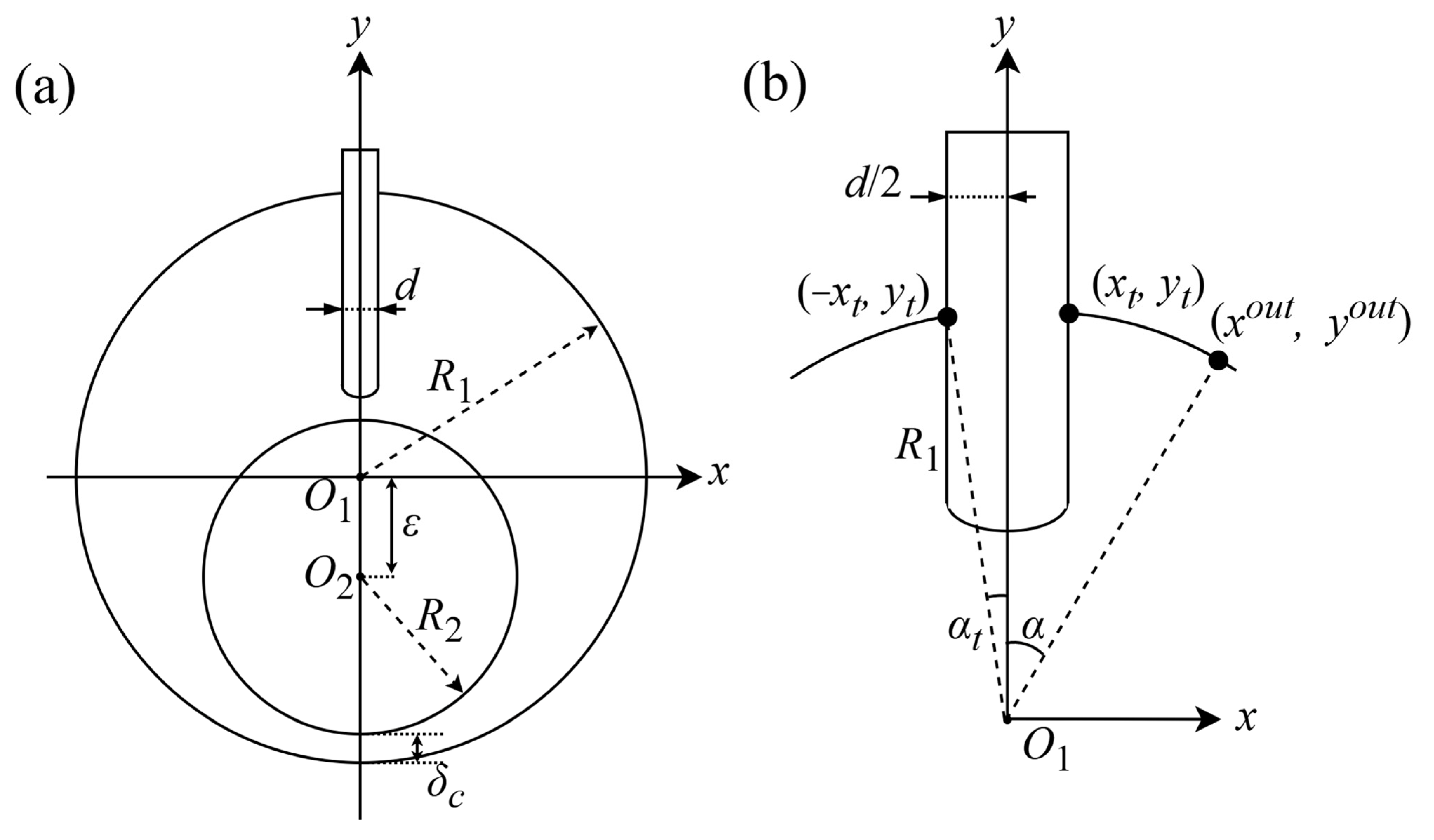
The cylinder profile consists of the cylinder inner wall and the portion of the vane located outside the slot, and its geometric definition is illustrated in Figure 3. The cylinder inner wall is a complete circle centered at the origin O 1 0,0 with a radius of R 1 , described parametrically as
x o u t = R 1 cos α , y o u t = R 1 sin α
where R 1 is the radius of the cylinder inner wall; α is the parametric angle of the outer boundary, defined in the counterclockwise direction over the prescribed angular range 0 2 π ; and x o u t , y o u t denotes the coordinates of an arbitrary point on the outer boundary, as shown in Figure 3a.
The geometric relationship between the vane slot and the cylinder inner wall is characterized by the vane slot half-angle α t , defined in Figure 3b. Because the vane thickness is d and the two end points of the vane slot are symmetric about the y axis, the vane slot half-angle α t satisfies
α t = arcsin d 2 R 1
As shown in Figure 3b, the coordinates of the left and right end points of the vane slot on the cylinder inner wall are x t ,   y t and x t ,   y t , respectively, where
x t = R 1 sin α t , y t = R 1 cos α t
These geometric quantities provide the basis for determining the boundary splitting and distributing the grid nodes in the subsequent grid generation procedure.

2.4. Rotor Profile

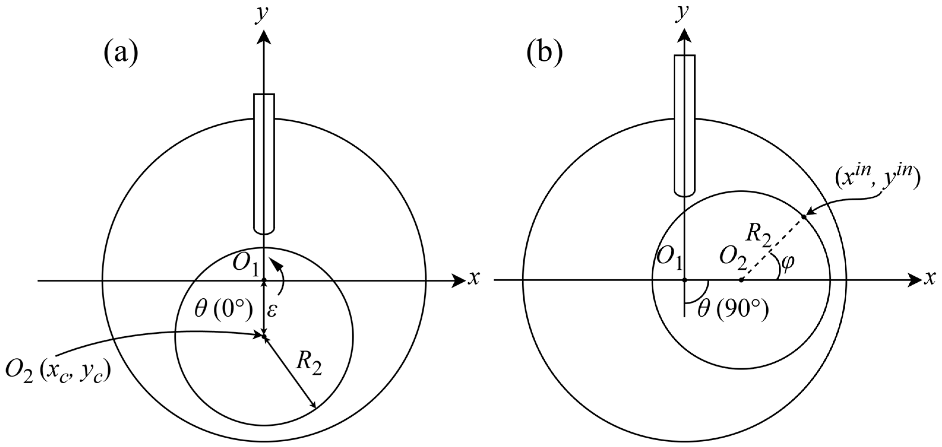
The rotor profile defines the inner boundary of the flow domain and is given by the outer surface of the rotor. As shown in Figure 4, the rotor is a cylindrical body of radius R 2 eccentrically positioned within the cylinder. The rotor radius is determined from the radius ratio κ as
R 2 = κ R 1 , 0 < κ < 1
The eccentric distance ε between the cylinder center O 1 and the rotor center O 2 is determined by
ε = ( 1 κ ) R 1 δ c
where δ c is the design clearance between the rotor outer wall and the cylinder inner wall which is introduced to prevent mechanical contact between the two components.
For an arbitrary rotor rotation angle θ , the coordinates of the rotor center x c and y c are given by
x c = ε cos θ π 2 , y c = ε sin θ π 2
The rotor outer wall is parametrically represented as
x i n = x c + R 2 cos φ , y i n = y c + R 2 sin φ
where φ is the parametric angle of the inner boundary (rotor outer wall), defined in the counterclockwise direction over the prescribed angular range 0 2 π ; x i n , y i n denotes the coordinates of an arbitrary point on the inner boundary.

2.5. Vane Profile

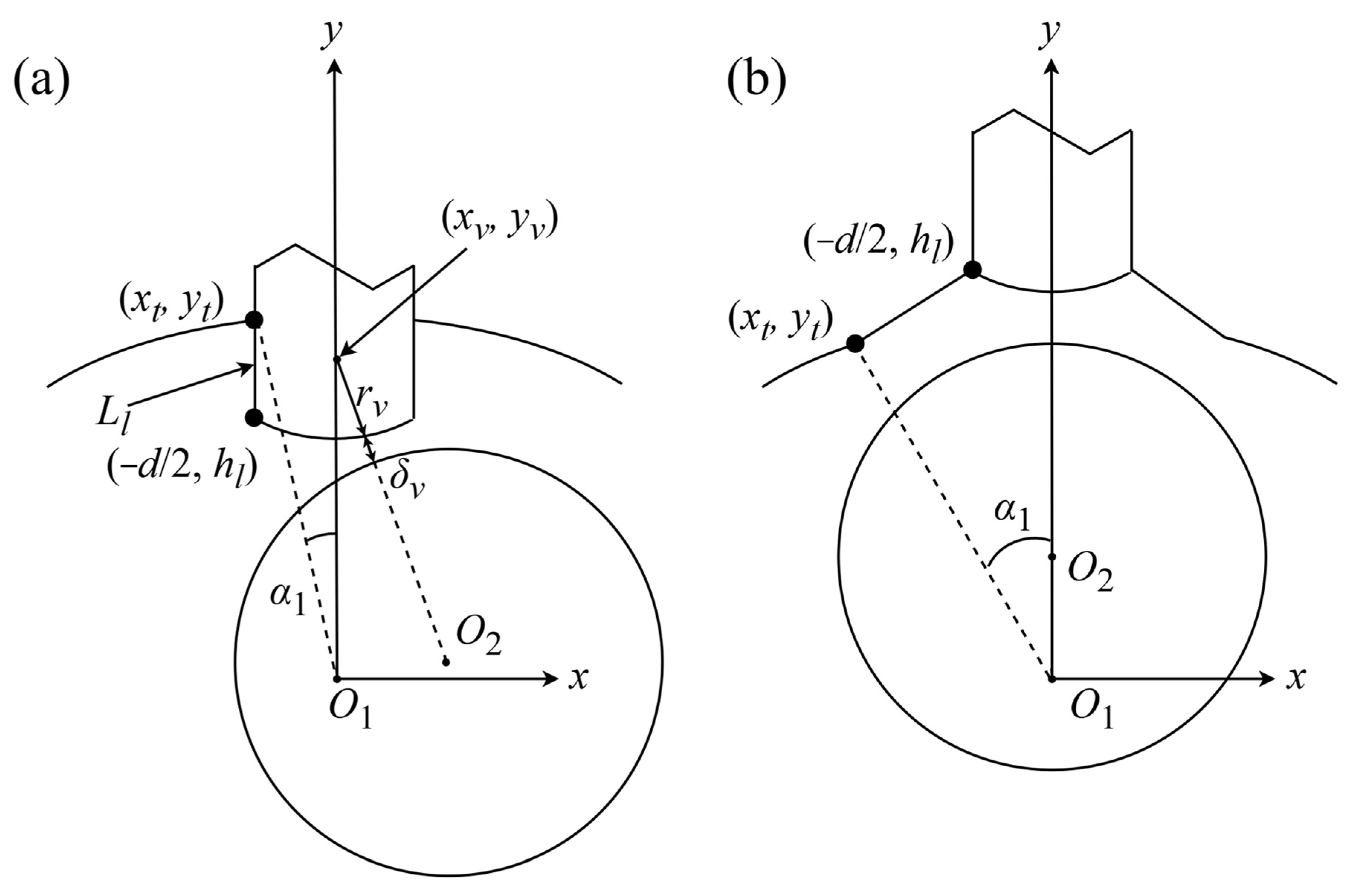
The vane tip profile is represented by an arc with radius r v , and the clearance between the vane tip and the rotor outer wall is denoted by δ v . The vane is symmetric about the y axis, and its geometric center lies on the y axis, as shown in Figure 5.
As shown in Figure 5a, the vane tip arc is tangent to the rotor outer wall, and its center is denoted by x v ,   y v . As the vane is symmetric about the y axis, x v   =   0 ; the vertical coordinate of the center is determined from the contact constraint between the vane tip and the rotor outer wall:
y v = y c + ( R 2 + δ v + r v ) 2 ( x v x c ) 2
Since the vane is axisymmetric, the vertical coordinates of the left and right endpoints, denoted as h l and h r , are equal and can be calculated as
h l = h r = y v r v 2 d 2 2
The protrusion lengths of the left and right sides of the vane are then defined as
L l = d 2 x t 2 + ( y t h l ) 2 L r = x t d 2 2 + ( y t h r ) 2
where L l is the protrusion length of the left side of the vane and L r is the protrusion length of the right side of the vane. For the axisymmetric vane considered here, L l = L r .

2.6. Short-Vane Correction

As shown in Figure 5b, when the rotor rotation angle approaches 180°, the vane progressively retracts into the vane slot, and L l and L r may decrease rapidly. If the original root half-angle is retained under these conditions, the mapping lines on both sides of the vane become concentrated within an extremely narrow region, causing node clustering, cell overlap and local grid degradation. To alleviate this problem, a short-vane criterion is introduced:
L min = min ( L l , L r ) < 0.06 R 1
where L m i n is the smaller of the two vane protrusion lengths.
When the above criterion is satisfied, the root half-angle α t is corrected according to
α t = 1.2 α t o
where α t o denotes the root half-angle before correction. The coordinates of the vane slot end points and the corresponding protrusion lengths are subsequently recalculated using the corrected value of α t . Geometrically, this treatment is equivalent to introducing a chamfer at the slot entrance and thereby enlarges the mappable angular range in the vicinity of the vane slot. The threshold value of 0.06 and the amplification factor of 1.2 are geometric control parameters selected on the basis of the resulting grid quality metrics.

3. Analytical Grid Generation

The proposed grid generation procedure is driven by the instantaneous rotor rotation angle θ and consists of four sequential steps: geometric updating, boundary splitting, adaptive split adjustment and three-dimensional grid construction. First, the rotor center and the center of the vane tip arc are determined from the rotor position, and the parametric equations of the cylinder inner wall and the rotor outer wall are established; the flow channel boundary is subsequently split into a vane region, transition regions and a core region according to the local geometric characteristics, and the start and end angles of each region are determined on the inner and outer boundaries. On this basis, the circumferential node number of each region is assigned adaptively from the mapped lengths of its inner and outer boundaries to provide higher local resolution in the internal clearance regions, while a normalization constraint keeps the total node number strictly equal to the prescribed value n c . After the node numbers have been determined, nodes are generated on the inner and outer boundaries of each region and assembled in circumferential order into a closed sequence; a two-dimensional face grid is then obtained by radial linear interpolation, and finally extruded uniformly in the axial direction into n a layers to form the three-dimensional structured grid.

3.1. Boundary Splitting

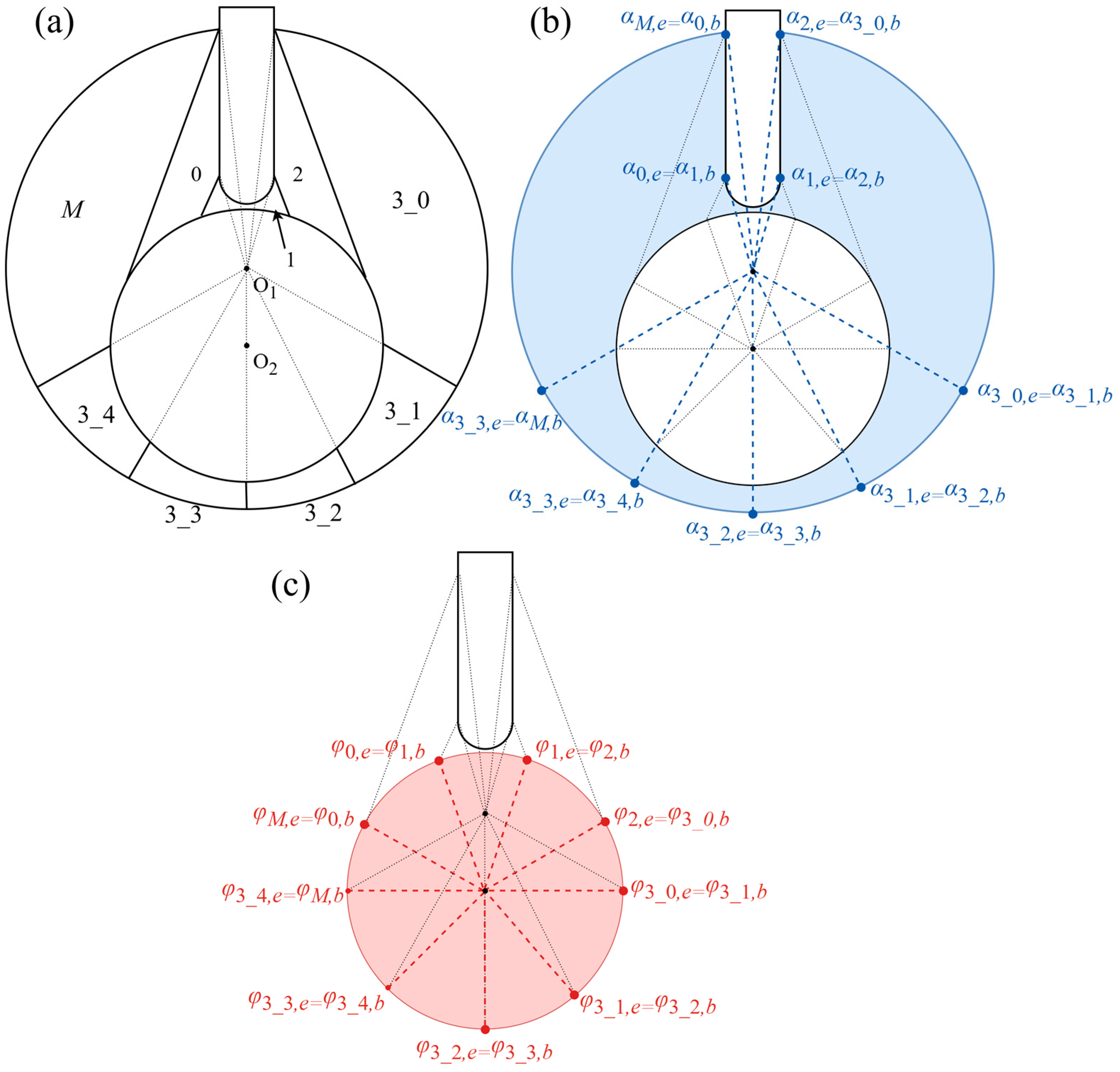
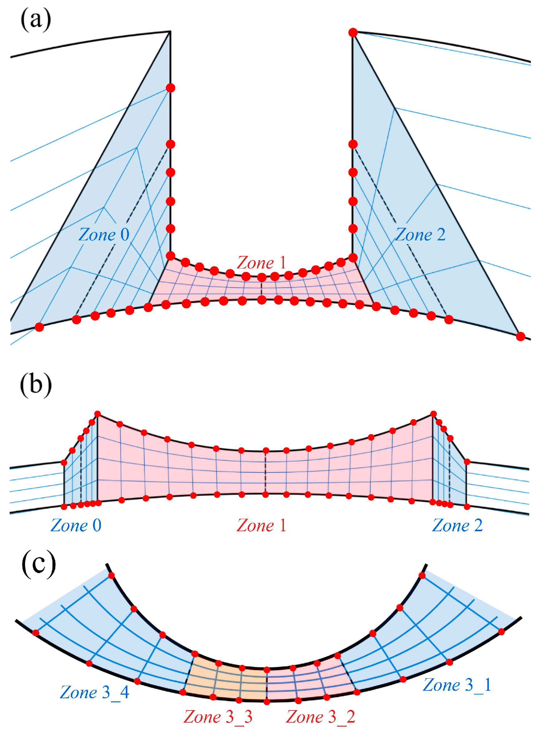
Since the geometric features near the vane are substantially more complex than those of the main arc channel away from the vane, a uniform node distribution over the entire boundary leads to insufficient resolution in the vane region or excessive nodes in less critical regions. Therefore, this paper splits the two-dimensional cross-sectional flow channel into the following three region types, as shown in Figure 6a: the vane region, the transition region and the core region. The vane region ( Z o n e   1 ) corresponds to the vane tip arc, where the geometric curvature varies sharply and a higher circumferential node density is required; the transition regions ( Z o n e   0 ,   Z o n e   2   a n d   Z o n e   M ) connect the vane region with the core region and provide a smooth geometric transition; the core region ( Z o n e   3 _ k ) corresponds to the arc channel away from the vane, whose geometry is relatively simple and whose node density is appropriately reduced. Z o n e   1 lies on the vane tip arc, Zone 0 and Zone 2 are located on its two sides, and Z o n e   M connects the left transition region to the core region; the main channel is further subdivided circumferentially into several sector subregions, Z o n e   3 _ k . The key idea of this splitting strategy is to separate the high-curvature region near the vane from the geometrically simpler main channel, so that the local node density matches the geometric complexity and the available nodes are concentrated in the internal clearance regions.
Each region is defined on both the inner and outer boundaries by a pair of start and end angles, where the start and end angles of the outer boundary are measured along the parametric angle α of the cylinder inner wall, and those of the inner boundary are measured along the parametric angle φ of the rotor outer wall. Figure 6b shows the circumferential splitting on the outer boundary (cylinder inner wall), where α i , b and α i , e respectively denote the start and end angles of Z o n e   i on the outer boundary; the junction between adjacent regions is marked in the form α i , e = α j , b i j , indicating that the end angle of Z o n e   i is the start angle of Z o n e   j . Similarly, Figure 6c shows the circumferential splitting on the inner boundary (rotor outer wall), corresponding to the start and end positions of each region on the rotor outer wall. The analytical expressions for the boundary angles of each region are given in Appendix A.

3.2. Adaptive Split Adjustment

As the rotor rotates, the start and end angles delimiting Z o n e   3 on the right side of the vane and Z o n e   4 on the left side change continuously, so the split must be adjusted dynamically to maintain a consistent topology. To this end, a reference direction pointing from the cylinder center O 1 to the rotor center O 2 is introduced. At θ = 0 the rotor is in its bottom-most position; the reference direction then coincides with the line joining the rotor center to the lowest point of the rotor and is aligned with the downward direction of the y axis. As the rotor rotates through the rotation angle θ , the reference direction rotates about O 1 by the same angle, and the reference angle is defined as the angle between the reference direction and the downward direction of the y axis:
φ r e f = θ
where φ r e f is the bottom reference angle of the rotor, measured from the downward direction of the y axis, and θ is the rotor rotation angle.
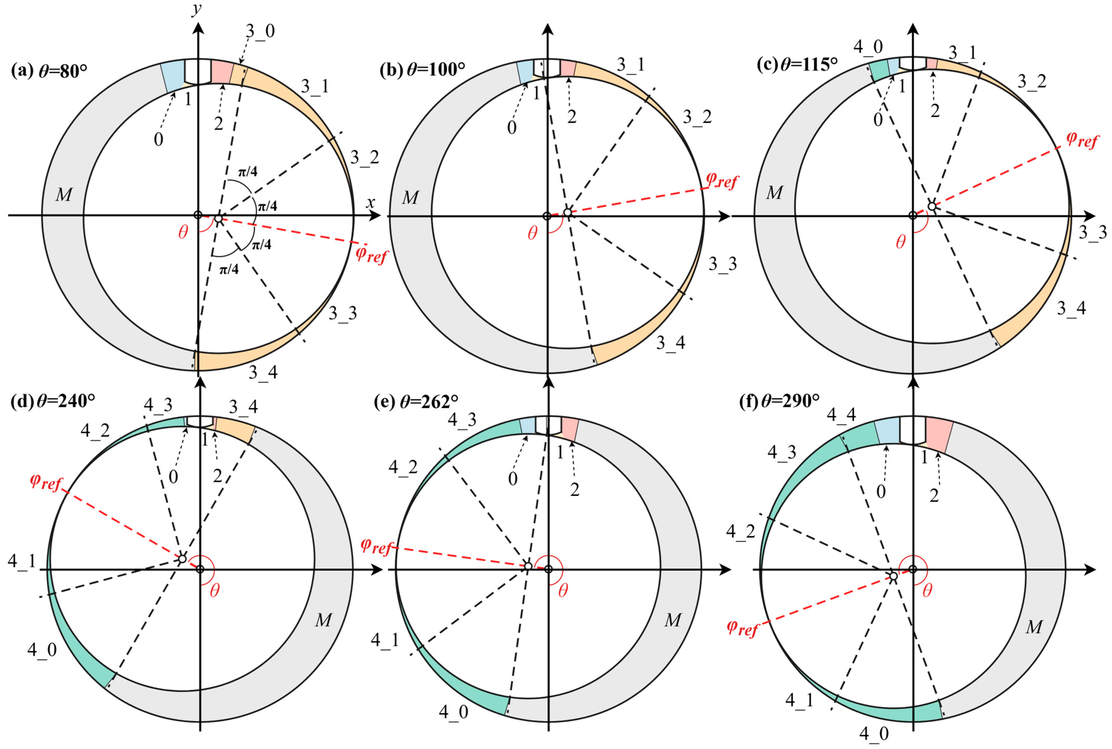
Taking φ r e f as the baseline, the five reference rays are arranged symmetrically about the reference direction, extending π / 2 to either side of it with a uniform spacing of π / 4 , and are labeled directly by the candidate terminal angles of the Z o n e   3 subregions on the inner boundary:
φ 3 _ k , e = φ ref + ( 2 k ) π 4 = θ + ( 2 k ) π 4 , k = 0 , 1 , , 4
Measured from the downward direction of the y axis, the five reference rays therefore lie at θ + π / 2 , θ + π / 4 , θ , θ π / 4 , and θ π / 2 , respectively. The central ray φ 3 _ 2 , e coincides with the reference direction φ r e f , while the outer rays φ 3 _ 0 , e and φ 3 _ 4 , e are offset from it by ± π / 2 . Adjacent reference rays are spaced π / 4 apart and rotate rigidly with the rotor. The adaptive hand-off between Z o n e   3 and Z o n e   4 is triggered by the crossings of these rays with two fixed angles on the inner boundary, φ 2 , e and φ 0 , b , the terminal angle of Z o n e   2 and the initial angle of Z o n e   0 , respectively, which are pinned by the vane roots and remain constant throughout the revolution. The splitting configurations at four representative rotation angles are illustrated in Figure 7.
Z o n e   3 _ k exists as an independent subregion while φ 3 _ k , e < φ 2 , e . Once φ 3 _ k , e rotates past φ 2 , e , Z o n e   3 _ k no longer satisfies the independent-existence condition: its node count is set to zero and it merges with the adjacent subregion. As shown in Figure 8a, all five subregions of Z o n e   3 are present at θ = 80 ° . After the reference ray φ 3 _ 0 , e crosses φ 2 , e at θ 87 ° , Z o n e   3 _ 0 is removed and its released angular interval is absorbed into the adjacent subregion Z o n e 3 _ 1 through the merging, while Z o n e s 3 _ 1 3 _ 4 remain active, keeping the boundary-angle sequence closed and continuous.
During this contraction, the angular interval [ φ 2 , e ,   φ 3 _ 4 , e ] occupied by Z o n e   3 on the inner boundary shrinks continuously as the rotor rotates. Because the total number of circumferential nodes n c is fixed, the nodes proportionally allotted to Z o n e   3 become compressed into a smaller interval, so the local node density rises, the grid spacing decreases, and the element aspect ratios deteriorate. Meanwhile, after the reference direction φ r e f sweeps past the vane, a new fan-shaped space gradually opens on the left side of the vane. To preserve the overall mesh quality without increasing the total node budget, this left-hand space is split independently into Z o n e 4 _ k . In this way, the node demand is transferred progressively from the contracting Z o n e   3 to the expanding Z o n e   4 , balancing the node densities on the two sides and preventing the right-hand main sector from degrading through excessive refinement.
Z o n e 4 _ k is numbered in the reverse order of Z o n e 3 _ k ( k = 0 , 1 , , 4 ), and its candidate subregions emerge one at a time as the reference rays sweep across the left side of the vane. Once φ 3 _ k , e reaches the inner-boundary angle φ 0 , b corresponding to the left endpoint of the vane slot, Z o n e 4 _ k begins to form and expands as the rotor continues to rotate until the next reference ray φ 3 _ k , e arrives. As shown in Figure 8c, φ 3 _ 0 , e crosses φ 0 , b at θ 109 ° , and Z o n e 4 _ 0 has just begun to form on the left side at θ = 115 ° .
The mechanism then repeats sequentially for k = 1 , 2 , 3 , 4 : Z o n e   3 loses its subregions one at a time while Z o n e   4 gains them, until the final hand-off. As shown in Figure 8d–f, only Z o n e   3 _ 4 remains at θ = 240 ° ; after φ 3 _ 4 , e crosses φ 2 , e at θ 251 ° , Z o n e   3 _ 4 is removed and merged, yet Z o n e   4 _ 4 has not appeared at θ = 262 ° , the gap being bridged by Z o n e   M ; once φ 3 _ 4 , e crosses φ 0 , b at θ 273 ° , Z o n e   4 _ 4 emerges at θ = 290 ° , the Z o n e   4 candidate subregions are complete, and the transfer of node demand from Z o n e   3 to Z o n e   4 is concluded.
With φ 2 , e and φ 0 , b acting as automatic switching thresholds, the procedure activates or deactivates the candidate subregions before their angular extent becomes vanishingly small, thereby preventing the generation of highly degenerate mesh cells. The detailed boundary formulation of Zone 4_k is provided in Appendix A.5.

3.3. Node Generation

After the boundary splitting is completed, structured grid nodes are generated on the two-dimensional cross section and subsequently extruded in the axial direction to form the three-dimensional grid. The procedure consists of three main operations: adaptive assignment of the circumferential node number for each region, calculation of the inner and outer-boundary node coordinates, and generation of the interior nodes by radial interpolation followed by axial extrusion.
The objective of the node number assignment is to match the local grid density with the local geometric complexity under a limited total node number. For an arbitrary region q , the mapped start-to-end length is defined as the Euclidean distance between the start points of the inner and outer boundaries l q , b , together with the Euclidean distance between their end points l q , e :
l q , b = x q , b o u t x q , b i n 2 + y q , b o u t y q , b i n 2 , l q , e = x q , e o u t x q , e i n 2 + y q , e o u t y q , e i n 2 .
A smaller mapped length indicates a smaller spacing between the inner and outer boundaries of the region, which usually requires a higher circumferential resolution to accurately capture the flow features within the clearance. The candidate circumferential node number of region q is defined as
n ~ q = 2 n r R 2 φ q , e φ q , b l q , e + l q , b
where n ~ q is the candidate circumferential node number of region q ; · is the ceiling function. This formula gives more nodes to regions with a longer arc length or a smaller inner–outer boundary spacing, while ensuring that each independent region is assigned at least one node. The sum of the candidate node numbers of all regions is usually not equal to the preset total circumferential node number n c . Let N r a w denote the total candidate node number:
N raw = q n ~ q
The node numbers of the regions other than Z o n e   1 are then scaled proportionally according to
n q = n ~ q N raw n c , q 1
The node number of Z o n e   1 is subsequently determined from the total node constraint:
n 1 = n c q 1 n q
If integer rounding causes n 1 to fall below its prescribed minimum, nodes are redistributed proportionally from Z o n e   3 _ k , Z o n e   4 _ k   a n d   Z o n e   M until the required resolution of the vane region is restored. The coordinate generation of the boundary, radial interior and axial nodes is detailed in Appendix B.
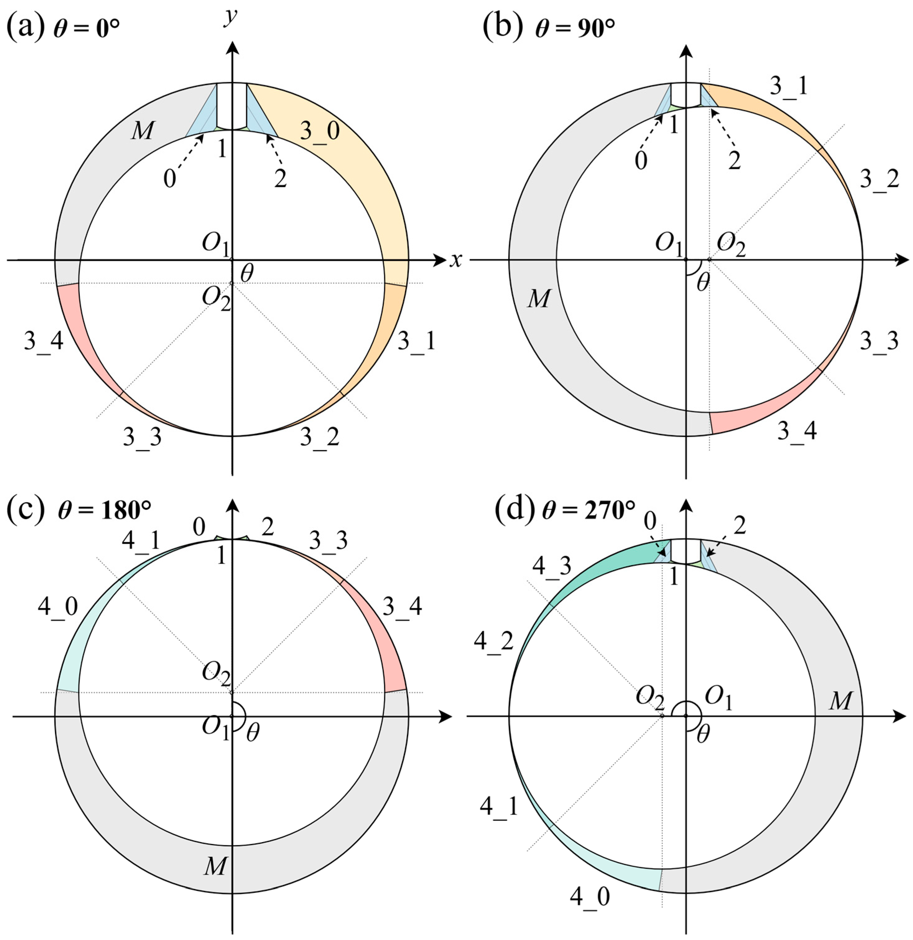
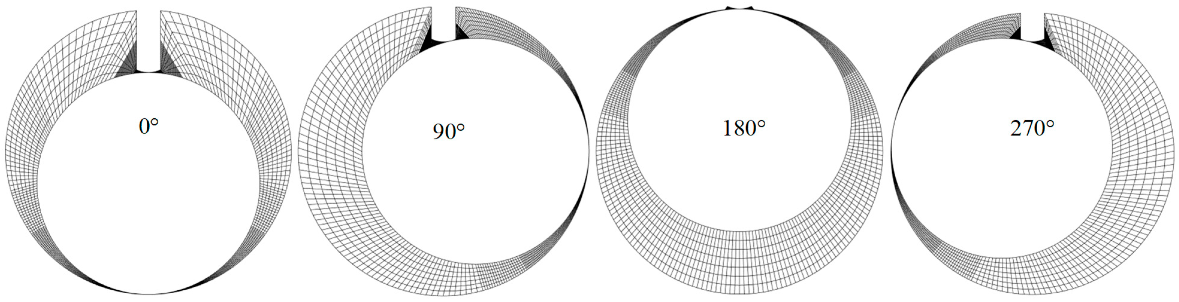
After completing grid generation, the three-dimensional structured mesh of the rotor fluid domain is finally obtained. Figure 9 presents the mesh distributions at four representative rotational angles within a complete operating cycle. At the initial rotational angle θ = 0 ° , local refinement is applied to the clearance between the vane tips and rotor outer surface and that between the rotor outer surface and the cylinder inner surface to ensure higher mesh quality in these critical areas. As the rotor rotates counterclockwise, adaptive split adjustments are performed within the range of θ = 90 ° 180 ° , during which Z o n e s   3 _ 0 ,   3 _ 1 , and 3 _ 2 are relocated to the left side of the vane to prevent mesh degradation on that side. Meanwhile, at θ = 180 ° , the short-vane correction is applied to the angle at the vane root. Subsequently, the remaining split adjustments are completed during the rotation from θ = 180 ° to 270 ° . Through the adopted zone-transition strategy and the short-vane correction, the proposed method guarantees high mesh quality at all rotational angles.

3.4. Applicability to Different Geometric Parameters

The proposed analytical grid-generation method uses the cylinder inner-wall radius, rotor radius, eccentricity, vane thickness, and vane-tip geometry as the primary inputs. For rolling-piston compressors with the same working-chamber topology, the boundary and interior nodes can be recalculated for different geometric parameters without reconstructing the overall grid topology. As shown in Table 1, Case 0 is the baseline configuration. Case 1 varies the radius ratio κ , Case 2 varies the vane-tip arc radius r v , and Case 3 varies the eccentricity ε . No negative-volume cells were observed in any case, indicating that the proposed method can accommodate these geometric variations while maintaining a valid computational mesh.
This applicability is limited to configurations with the same basic working-chamber topology. Significant changes in the vane-tip profile, the introduction of multiple vanes, or changes requiring a different domain partition would require new local boundary mappings and partitioning relationships.

3.5. Advantages and Limitations of the Proposed Grid-Generation Method

Compared with dynamic mesh approaches that rely on solver-side smoothing, reconstruction, or remeshing, the proposed analytical grid-generation method adopts a different mesh-update strategy. The nodal coordinates are calculated outside the CFD solver from predefined analytical geometric relationships and are directly updated during the simulation, without additional mesh smoothing or local reconstruction at each time step. Table 2 provides a qualitative comparison of the two approaches in terms of grid generation, solver dependency, grid topology, convergence behavior, numerical stability, numerical error, computational cost, and geometric adaptability.
As shown in Table 2, a major advantage of the proposed method is the deterministic and repeatable mapping of grid motion. When the working-chamber topology remains unchanged, the grid connectivity is preserved throughout the rotor motion, avoiding repeated reconstruction or topology changes during the CFD solution. This reduces solver-side mesh-processing operations and may also reduce local convergence disturbances associated with mesh updates. Because the grid coordinates are determined in advance, the method is less dependent on built-in dynamic mesh, smoothing, and remeshing functions. Its computational advantage is mainly associated with grid preprocessing and mesh updating during the solution, while the quantitative comparison of preprocessing time is presented in Section 4.3. It should be emphasized that the proposed grid-generation strategy does not inherently reduce CFD discretization error, which remains dependent on grid resolution, time-step size, discretization schemes, and the adopted physical models.
The main limitation of the method is its dependence on predefined geometric relationships and domain partitioning. Variations in the radius ratio, eccentricity, or vane-tip geometry can be accommodated by recalculating the nodal positions as long as the basic working-chamber topology is preserved. However, substantial changes in the vane configuration, chamber topology, or domain partitioning require reconstruction of the corresponding analytical mappings. In addition, because no additional iterative mesh smoothing or orthogonalization is employed, local grid quality may still deteriorate at certain rotor positions. The proposed method is therefore more suitable for rolling-piston compressors with well-defined motion and unchanged working-chamber topology than for general moving-boundary problems. Since the geometries, grid resolutions, numerical settings, and computational platforms reported in the literature are not directly comparable, the present study does not quantitatively rank different grid-handling methods in terms of error level, convergence rate, or computational time; instead, the comparison focuses on their numerical mechanisms and computational workflows.

4. Numerical Case Study

This section evaluates the proposed analytical grid generation method by carrying out CFD simulations of an RPC.

4.1. Governing Equations

The flow and heat transfer inside the RPC are governed by the three-dimensional, unsteady, compressible Navier–Stokes equations, whose mass and momentum conservation are expressed as
ρ t + ρ u u g = S m
ρ u t + ρ u u u g = p + τ ¯ ¯ + ρ g + F
where ρ is the density, u is the velocity vector, p is the static pressure, τ is the viscous stress tensor, g is the gravitational acceleration, F is an external body force, and S m is the mass source term. For a Newtonian fluid, the viscous stress tensor is closed by
τ ¯ ¯ = μ u + u T 2 3 u I
where μ is the dynamic viscosity and I is the unit tensor, and the term containing the divergence of the velocity accounts for the effect of volume dilation. Energy conservation is formulated in terms of the specific enthalpy. Since the working fluid is a single-component refrigerant, the mass-fraction-weighted summation reduces to the enthalpy of the single species, which is obtained by integrating its specific heat at constant pressure from a reference temperature,
h j = T r e f T C p , j d T
The specific internal energy is then obtained by subtracting the pressure work from the enthalpy:
e = h p o p + p ρ
The energy conservation equation is therefore written as
t ρ e + | u | 2 2 + ρ u u g h + | u | 2 2 = λ eff T j h j J j + τ ¯ ¯ eff u + S h
where e is the specific internal energy, λ eff is the effective thermal conductivity, T is the temperature, J j is the diffusion mass flux of species j , τ eff is the effective stress tensor including the turbulent contribution, and S h is a volumetric heat source. Because the rotor domain deforms during the simulation, the conservation equations are solved in their arbitrary Lagrangian–Eulerian (ALE) form, and the mesh motion must satisfy the geometric conservation law
d d t V d V = A u g d A
where u g is the local grid velocity. In the present approach u g is not evaluated by a solver-side mesh-motion algorithm but is prescribed analytically. The mesh generator supplies the nodal coordinates of every time step of a complete revolution before the simulation is started, and the user-defined function assigns these coordinates to the corresponding nodes at each time step. Because the nodal connectivity and the cell topology remain unchanged throughout the revolution and only the node positions are updated, the change in the control volume is exactly the volume swept by its moving faces; the geometric conservation law is therefore satisfied identically at the discrete level, and the mesh motion introduces no spurious mass source [13,30].

4.2. Geometric Configuration

A representative RPC was selected as the numerical case. Its geometric dimensions incorporate the key structural features commonly encountered in RPCs, including the radial clearance, vane thickness, and radius of the vane-tip arc. Key geometric parameters, such as the rotor-to-cylinder radius ratio and eccentricity, were kept consistent with those of the experimental model reported in Ref. [6]. The principal geometric parameters adopted in the present numerical case are summarized in Table 3.

4.3. Grid Generation

The rotor and port meshes of the RPC are shown in Figure 10. The compressor consists of one suction port and two discharge ports. The suction process takes place through a single radial port, whereas the two discharge ports are symmetrically arranged on the two end walls and are connected to the radial discharge pipe through inclined passages. Non-conformal sliding interfaces are defined along the cylinder surface to enable mass and energy transfer between the rotor fluid domain and both the suction and discharge ports.
The rotor mesh was generated using the developed analytical grid generation method, while the port meshes were generated using ANSYS ICEM CFD 2022R1. The mesh quality statistics of the port domains are summarized in Table 4, with a total of 81,715 cells in all port domains. As summarized in Table 5, for the conventional workflow, generating and checking meshes at 360 rotor positions over a complete 0–360° cycle requires approximately 48 h, with most of this time associated with repetitive manual mesh generation, quality inspection, and local adjustment rather than computer execution time. In contrast, once the initial geometric and mesh parameters are specified, the proposed analytical grid generation method automatically computes the nodal positions for all 360 rotor positions in MATLAB R2021a, reducing the preprocessing time to approximately 54 s, corresponding to a reduction of about 99.97%. The reported preprocessing times refer exclusively to mesh preparation and exclude the subsequent CFD solution time.
As shown in Figure 11, the mesh quality in the rotor region exhibits a clear periodic variation with rotor angle. The minimum orthogonal quality decreases to relatively low values near 90° and 270°, whereas it remains comparatively high over the range of 135–225° and reaches a peak near 180°. The maximum aspect ratio shows an approximately opposite trend, attaining its highest values near 90° and 270° while remaining relatively low between 135° and 225°. The maximum skewness remains relatively large over the ranges of 0–135° and 225–360°, decreases markedly within the intermediate angular range, and exhibits a local fluctuation near 180°. Overall, the three mesh-quality metrics vary periodically with rotor motion, indicating that local geometric deformation has a pronounced influence on the mesh quality in the rotor region. Despite the local deterioration in mesh quality at certain rotor angles, no negative-volume cells were detected throughout the complete 0–360° dynamic-mesh update process, indicating that the generated mesh remained geometrically valid without cell inversion over the entire rotation cycle. A separate minimum-Jacobian metric was not directly available in the present Fluent post-processing. Therefore, the negative-volume-cell check was used only as an additional assessment of mesh validity and was not considered equivalent to a Jacobian evaluation.

4.4. Coupling Grid Generation Method with CFD Solver

Figure 12 outlines the complete numerical workflow. All input parameters—the geometric configuration, the boundary discretization scheme, and the nodal distribution—are defined first; the principal geometric parameters of the RPC are listed in Table 3. Two-dimensional meshes are then generated for every time step of a full rotor revolution through boundary generation, boundary discretization, and internal node allocation. The mesh at the initial time step is extruded to form the three-dimensional baseline mesh at the initial rotor position in the CFD solver. The procedure yields a mesh database containing the nodal coordinates of every time step, stored in a series of data files and read sequentially by the CFD solver as the simulation advances. The generated mesh dataset is then coupled with the commercial CFD solver. The coupling procedure is described in detail in Ref. [22], and the parallel implementation of the user-defined function (UDF) is presented in Ref. [30]. After the baseline mesh is loaded into the FLUENT solver, the parallel UDF performs a mapping operation at the first time step, establishing a one-to-one correspondence between the solver mesh nodes and the nodal coordinates stored in the data files. It then reads the coordinates at each time step and updates the mesh dynamically throughout the simulation. The rotor mesh is connected to the stationary fluid domains through non-conformal interfaces.

4.5. Numerical Model Setup

The numerical simulations were performed with the ANSYS Fluent 2022R1 solver, and the principal model settings are listed in Table 6. R32 was selected as the working fluid. During the calculation, the pressure dependence of the specific heat is recovered through an energy-integration procedure within each computational cell, which requires the real-gas equation of state. The thermodynamic state of the working fluid is therefore described by the Aungier–Redlich–Kwong (ARK) real-gas equation of state [31], which also closes the governing equations,
p = R T v b + c a ( T ) v ( v + b )
where R is the specific gas constant, v is the specific volume, and a ( T ) , b and c are model parameters. The specific volume is related to the density by Equation (29), and the temperature-dependent attraction parameter is given by Equation (30).
v = 1 ρ
a ( T ) = a 0 T c T n
in which the model constants are determined from the critical properties of the fluid as
a 0 = 0.42747 R 2 T c 2 p c
b = 0.08664 R T c p c
c = R T c p c + a 0 / v c ( v c + b ) + b v c
where T c , p c and v c are the critical temperature, critical pressure and critical specific volume, respectively, and n is a model exponent. The enthalpy of the real gas is decomposed into an ideal-gas contribution and a departure term,
h = h i d e a l + Δ h
where the departure enthalpy is evaluated from
Δ h = p v R T a ( T ) ( 1 + n ) b ln v + b v
while the specific heat at constant pressure is corrected by a departure term, and the ideal-gas contribution is represented by a fourth-order polynomial in temperature,
c p = c p , i d e a l + Δ c p
c p , i d e a l = C 1 + C 2 T + C 3 T 2 + C 4 T 3 + C 5 T 4
whose coefficients C 1 to C 5 are determined from the REFPROP database. Finally, the transport properties of the working fluid are evaluated from
μ = f ( T , p )
where the dynamic viscosity is tabulated as a function of temperature and pressure, and the thermal conductivity is obtained from the modified Eucken relation
λ = ( c p + 1.25 R ) μ
where c p is the specific heat of R32 at constant pressure and is expressed as a fourth-order polynomial in temperature, as given in Equation (40). The coefficients of this polynomial correspond to the zero-pressure ideal-gas state and were obtained from REFPROP. The critical pressure and critical temperature were set to 57.06 bar and 351.255 K, respectively, and a property lookup table was generated over the temperature range of 267–400 K.
C P 0 ( T ) = 8 × 10 9 T 4 2 × 10 5 T 3 + 1.43 × 10 2 T 2 2.9533 T + 863
The turbulence closure is provided by the shear-stress transport (SST) k ω model, which solves two additional transport equations for the turbulent kinetic energy k and the specific dissipation rate ω :
( ρ k ) t + ( ρ k u i ) x i = x j Γ k k x j + G k Y k
( ρ ω ) t + ( ρ ω u i ) x i = x j Γ ω ω x j + G ω Y ω + D ω
where G k and G ω denote the production of k and ω , Y k and Y ω their dissipation due to turbulence, D ω the cross-diffusion term, and Γ k and Γ ω the effective diffusivities of k and ω , which are computed from the turbulent viscosity as
Γ k = μ + μ t σ k , Γ ω = μ + μ t σ ω
in which the turbulent viscosity is evaluated from
μ t = ρ k ω max 1 α * , S F 2 a 1 ω 1
where S is the modulus of the strain-rate tensor, y w is the distance to the nearest wall, and the blending functions are
F 2 = tanh Φ 2 2 , Φ 2 = max 2 k 0.09 ω y w ,   500 μ ρ y w 2 ω
The remaining model constants and blending functions follow the standard SST formulation of Menter [32]. Together with the closure relations above, the governing equations of Section 4.1 form the complete mathematical model solved in the CFD simulations.
As shown in Table 6, the numerical settings adopted in this study were determined by balancing computational accuracy, numerical stability, and computational efficiency. Considering the stability and convergence requirements of three-dimensional transient simulations, a first-order upwind scheme was employed for spatial discretization, while a first-order implicit scheme was used for temporal discretization. It should be noted that first-order schemes may introduce a certain degree of numerical dissipation, thereby reducing the resolution of local flow structures. However, the present study mainly focuses on the overall evolution of the working-chamber volume and the corresponding pressure variation, and the adopted discretization schemes are therefore considered adequate for the primary objectives of this work. To further simplify the numerical model and reduce the computational cost, end-face leakage, the sealing effect of lubricating oil and the associated heat-transfer processes were not considered, and conjugate heat transfer between the moving components and the refrigerant was also neglected. These physical simplifications may affect the local pressure response and thermodynamic behavior to some extent, and their influence is further discussed in the subsequent experimental validation and error analysis.
To validate the numerical model and assess the applicability of the proposed analytical grid generation method at different operating speeds, the 80 Hz and 120 Hz operating conditions reported in Ref. [6] were selected for comparison. As summarized in Table 7, the cylinder inner-wall radius, rotor radius, and eccentricity adopted in the present simulation are consistent with the experimental geometry within the reported precision, and R32 was used as the working fluid in both the experiment and simulation. The corresponding rotational speeds were 4800 rpm and 7200 rpm for the 80 Hz and 120 Hz cases, respectively. For both cases, the suction port was specified as a pressure-inlet boundary with a pressure of 0.5 MPa and a temperature of 267.15 K, whereas the discharge port was specified as a pressure-outlet boundary with a pressure of 2.1 MPa, consistent with the reference experimental conditions.
At the start of the simulation, the fluid domain was initialized using the suction-side pressure and temperature conditions. All solid walls of the compressor were treated as no-slip, adiabatic boundaries, with the wall heat flux set to zero. The rotor dynamic-mesh region was connected to the suction and discharge port regions through non-conformal mesh interfaces, through which mass, momentum, and energy fluxes were transferred. The 80 Hz case was used for baseline validation, while the 120 Hz case was employed to further assess the applicability of the proposed method at a higher rotational speed.
The iterative convergence within each physical time step was assessed using a combination of the scaled residuals of the governing equations and the chamber-averaged pressure and temperature. The residual convergence criteria for the governing equations are listed in Table 6. A physical time step was considered converged when the residuals satisfied the prescribed criteria and the chamber-averaged pressure and temperature no longer exhibited noticeable variations during the inner iterations, after which the calculation proceeded to the next physical time step. This combined criterion based on both residuals and monitored physical quantities helps avoid judging transient convergence solely from residual behavior.
The transient CFD simulations at 80 Hz and 120 Hz were performed over one complete rotor revolution from 0° to 360°. The analysis focuses on the transient evolution of the working chamber within this rotation cycle, including the corresponding pressure–volume behavior. Since successive rotation cycles were not considered in the present simulations, cycle-to-cycle periodic convergence was not evaluated. The reported results therefore correspond to the transient response under the prescribed initial and operating conditions.
The experimental p–V data used for validation were extracted from the published experimental curves in Ref. [6] using an image digitization tool. To quantitatively evaluate the agreement between the numerical and experimental results, the mean absolute percentage error (MAPE) was adopted as the primary error metric. Because the sampling locations of the experimental and numerical p–V data were not identical, the correspondence among the numerical pressure-monitoring time, rotor angle, and working-chamber volume was first rechecked, and a consistent physical phase reference was established before the error calculation. Within the corresponding physical stage, the numerical pressure was then linearly interpolated as a function of working-chamber volume to obtain simulated pressure values at the experimental sampling volumes. This procedure was used only to establish the correct physical correspondence between pressure and volume, without modifying any original pressure values. The MAPE is defined as
M A P E = 1 N i = 1 N p i , s i m p i , e x p p i , e x p   ×   100 %
where p i , s i m and p i , e x p denote the simulated and experimental pressures, respectively, at the i -th corresponding volume location, and N is the total number of data points included in the comparison. This procedure helps avoid additional nonphysical comparison bias arising from inconsistent sampling locations or pressure–volume correspondence and provides a consistent basis for quantitative comparison across different operating speeds.

5. Results

5.1. Grid Independence Test

To evaluate the influence of grid resolution on the numerical results, independent refinement studies were conducted in the radial and axial directions, with the discharge temperature selected as the monitoring parameter. As shown in Table 8, when the number of radial cells was increased from 4 to 7 and 12, the discharge temperature decreased from 310.814 K to 308.975 K and 308.569 K, respectively, while the relative difference between successive grids decreased from 0.595% to 0.132%. Similarly, as summarized in Table 9, increasing the number of axial cells from 20 to 30 and 45 resulted in discharge temperatures of 310.763 K, 308.975 K, and 308.682 K, respectively, with the relative difference decreasing from 0.579% to 0.095%. These results demonstrate that the discharge temperature becomes progressively less sensitive to further grid refinement in both directions, indicating a clear convergence trend.
To further quantify the discretization uncertainty, Richardson extrapolation and the Grid Convergence Index (GCI) method were applied, with the corresponding results presented in Table 10. The Richardson-extrapolated discharge temperatures for the radial and axial refinement studies were 308.443 K and 308.625 K, respectively, both of which were close to the corresponding fine-grid solutions. The fine-grid G C I 21 values were 0.051% for radial refinement and 0.023% for axial refinement, both below 0.1%. These low fine-grid GCI values indicate that the solutions approach grid convergence as the mesh is refined.
Considering that the differences in discharge temperature between the medium and fine grids were only 0.132% for radial refinement and 0.095% for axial refinement, the medium grid with 7 radial cells and 30 axial cells was adopted for the subsequent simulations as a compromise between numerical accuracy and computational cost.
In Table 10, the subscripts 1, 2, and 3 denote the fine, medium, and coarse grids, respectively. Accordingly, r21 and r32 represent the refinement ratios, while G C I 21 and G C I 32 represent the Grid Convergence Indices for the fine–medium and medium–coarse grid pairs, respectively.

5.2. Experimental Validation

Ref. [6] conducted an experimental and mathematical modeling study on a high-speed RPC over a wide range of rotational speeds, with particular attention to compressor performance and the pressure variation within the compression chamber. To validate the effectiveness of the proposed grid generation method and the numerical model supported by the generated mesh, the simulated pressure–volume curve during the compression stage was compared with the experimental data reported in Ref. [6], as shown in Figure 13. The horizontal axis represents the compression-chamber volume, whereas the vertical axis represents the chamber pressure. The solid black lines denote the simulated results, and the dashed blue lines represent the experimental data. The numerical results reproduce the overall evolution of the experimental p–V curves at both operating speeds. For the 80 Hz case (Figure 13a), the simulated pressure shows reasonable agreement with the experimental data over most of the compression process, although an overprediction is observed in the high-pressure region. For the 120 Hz case (Figure 13b), the numerical results reproduce the overall trend of the experimental pressure evolution, while a more pronounced deviation occurs near the pressure peak. The mean absolute percentage errors (MAPEs) are approximately 6.30% and 7.42% for the 80 and 120 Hz cases, respectively. Within the main common p-V range, the corresponding maximum pointwise relative errors are approximately 12.7% and 21.0%, respectively.
Near the onset of discharge, corresponding to chamber volumes of approximately 2–3 cm3, the simulations exhibit a transient pressure rise. This behavior is mainly associated with the numerical treatment in which the discharge boundary is instantaneously switched from a wall boundary to a pressure-outlet boundary. In the experiments, the pressure response in this region is additionally influenced by discharge-valve dynamics, throttling through the discharge passage, and pressure pulsations in the muffler chamber. The remaining discrepancies between the numerical and experimental results may also be attributed to several physical simplifications adopted in the present model. In an actual rolling-piston compressor, the pressure evolution is affected by leakage, oil-sealing effects, wall heat transfer, and discharge-valve dynamics. Lubricating oil within the end-face and vane-slot clearances provides a certain sealing effect, whereas oil–refrigerant interactions and end-face leakage are not explicitly modeled in the present study. In addition, a complete conjugate heat-transfer model and a dynamic discharge-valve model are not included; consequently, the transient heat exchange between the refrigerant and the solid components, as well as the actual opening and closing behavior of the discharge valve, cannot be fully reproduced. The influence of the simplified discharge-valve treatment is expected to be more pronounced near the onset of discharge, whereas the simplifications associated with leakage and heat transfer may affect the chamber mass and pressure evolution throughout the compression process. The deviations observed in the present simulations are therefore more reasonably attributed to the combined effects of these physical simplifications rather than to any single factor. Quantifying the individual contribution of each mechanism will require further sensitivity analyses and more comprehensive physical models.
Despite these localized discrepancies, the simulated p V curves show reasonable agreement with the experimental measurements at both rotational speeds. The physical simplifications discussed above may also affect global compressor performance parameters, such as mass flow rate and volumetric efficiency. Therefore, quantitative validation of these quantities was not included in the present study and will be considered in future work using more complete leakage, heat-transfer, and discharge-valve models. Overall, the results indicate that the analytical grid generated by the proposed method can represent the evolution of the working-chamber geometry and provide a suitable mesh framework for transient CFD simulations of the compression and discharge processes in rolling-piston compressors.

5.3. Sensitivity Analysis of Spatial Discretization Order

To further evaluate the influence of the spatial discretization order on the numerical results, a limited sensitivity analysis was conducted for the 80 Hz operating condition. The computational mesh, time-step size, boundary conditions, initial conditions, and convergence criteria were kept unchanged, while the first-order upwind schemes were replaced with the corresponding second-order upwind schemes. The resulting p–V curves were then compared with the experimental data. As shown in Figure 14, both discretization schemes reproduce the overall evolution of the experimental p–V curve reasonably well. The two simulated curves nearly overlap during most of the low- and intermediate-pressure compression stages, whereas more noticeable differences occur in the high-pressure region at approximately 1–3 cm3. In this region, the second-order scheme reduces the local pressure overprediction observed with the first-order scheme and shows better overall agreement with the experimental data.
Quantitatively, the mean absolute percentage errors (MAPEs) obtained with the first- and second-order upwind schemes are 6.30% and 5.26%, respectively. However, within the main common p–V range, the corresponding maximum pointwise relative errors are 12.70% and 12.98%, indicating that the second-order scheme mainly improves the overall pressure prediction, while providing only limited improvement in the maximum local deviation. Overall, increasing the spatial discretization order moderately reduces the average prediction error without altering the primary physical trend of chamber pressure variation with volume. Since the present study focuses on the analytical grid generation method and its capability to describe the overall compression process, the first-order upwind scheme is retained as the baseline spatial discretization scheme, considering the numerical stability and computational cost associated with three-dimensional transient dynamic-mesh simulations.

5.4. Time-Step Sensitivity Analysis

To evaluate the influence of time-step size on the numerical results, simulations were performed at 80 Hz using rotor-angle increments of 1 , 0.5 , and 0.25 , while the computational mesh, physical models, boundary conditions, and other numerical settings were kept unchanged. As shown in Figure 15, the p V curves obtained with the three time steps exhibit similar overall trends during most of the compression process, indicating that time-step refinement does not alter the fundamental chamber-pressure evolution with volume. The main differences are concentrated in the high-pressure region at approximately 1–3 cm3 where the smaller time steps resolve more local pressure variations. Meanwhile, more pronounced local pressure oscillations are observed for the 0.25 case in the high-pressure region and at several stages of compression.
Quantitatively, the MAPE values for the 1 , 0.5 , and 0.25 cases are 6.30%, 5.86%, and 2.99%, respectively, indicating an improvement in the overall pressure prediction with decreasing time-step size. However, the corresponding maximum pointwise relative errors are 12.70%, 13.38%, and 12.63%, respectively, and therefore do not decrease monotonically with time-step refinement. This indicates that time-step refinement primarily improves the average agreement with the experimental data, while its influence on the maximum local deviation is relatively limited.
Overall, all three time steps reproduce a consistent p V evolution. Smaller time steps reduce the average prediction error but increase the computational cost, while the 0.25 case also exhibits more pronounced local pressure oscillations. Since the present study primarily focuses on the proposed analytical grid-generation method and its numerical performance over a complete working cycle, the 1 rotor-angle increment was retained as the baseline time step because it adequately reproduces the overall pressure evolution at a lower computational cost.

5.5. Flow Field Analysis

The internal pressure field of the compressor exhibits a clear periodic variation over the operating cycle. Figure 16 shows the pressure distributions in the working chambers of the RPC at rotor angles of 0°, 90°, 180°, and 270°, with the pressure ranging from 1 to 24 bar. At 180° and 270°, most of the chamber remains at a relatively low and nearly uniform pressure of approximately 5–7 bar, indicating that the refrigerant has undergone only limited compression at these stages. As the rotor moves to 0°, the chamber volume decreases and the pressure rises, accompanied by a more distinct circumferential pressure gradient. This behavior is mainly caused by the progressive compression of the trapped refrigerant and the resulting pressure redistribution within the moving chamber.
At 90°, a localized high-pressure region of approximately 20–22 bar develops near the discharge side, while the remaining chamber retains a considerably lower pressure. This indicates that the refrigerant has reached the final stage of compression and that the pressure increase becomes concentrated near the discharge region as the chamber volume approaches its minimum. The pronounced pressure contrast across the vane and narrow-clearance regions also suggests that pressure equalization between adjacent chambers remains limited. Overall, the pressure evolution is strongly governed by the periodic variation in chamber volume, with the pressure increasing progressively as the trapped refrigerant is compressed and becoming concentrated near the discharge side toward the end of the compression process.
Figure 17 shows the temperature distributions in the RPC at rotor angles of 0°, 90°, 180°, and 270°, with the temperature ranging from 220 to 370 K. At 0°, a clear temperature difference exists between the two working chambers, with the compression side exhibiting a higher temperature because of the progressive reduction in chamber volume. At 90°, a localized high-temperature region of approximately 350–370 K appears near the discharge side, indicating intensified compression heating as the chamber approaches the discharge stage.
At 180°, a relatively broad high-temperature region develops in the lower part of the chamber, with temperatures of approximately 300–340 K. This distribution reflects the combined effects of compression and internal redistribution of thermal energy within the moving chamber. In contrast, at 270°, the chamber temperature decreases markedly and remains mostly within approximately 240–270 K, mainly because of the larger chamber volume and the continuous intake of low-temperature refrigerant. Overall, the temperature field is strongly coupled with the periodic variation in chamber volume: compression causes the refrigerant temperature to increase, whereas chamber expansion and suction maintain a relatively low temperature. Local temperature gradients near the vane tip and minimum-clearance regions also indicate additional mixing between refrigerant streams with different thermal states.
Figure 18 shows the velocity contours and streamline distributions in the working chambers of the RPC at rotor angles of 0°, 90°, 180°, and 270°. At 0°, the streamlines are relatively regular along the chamber, with only limited local deflection near the vane region, indicating a comparatively stable internal flow. At 90°, pronounced recirculation and vortical structures develop near the discharge passage and the vane region. These structures are mainly caused by the rapid redirection and acceleration of the refrigerant as it approaches the restricted discharge flow path, resulting in stronger momentum exchange and local flow losses.
At 180°, a distinct large-scale vortex appears in the lower part of the working chamber, accompanied by noticeable streamline curvature. This behavior is associated with the rapid variation in chamber geometry and the resulting redistribution of the internal flow. By contrast, at 270°, the streamlines become more uniformly distributed in the circumferential direction and the flow field is comparatively smooth. Overall, the internal flow pattern varies markedly with rotor position. The strongest flow disturbances occur when the refrigerant experiences rapid acceleration, flow redirection, or geometric restriction, particularly near the discharge passage and the vane region.

6. Conclusions

This study developed an analytical grid-generation method based on user-defined nodal displacement (UDND) for transient CFD simulations of rolling-piston compressors (RPCs). According to the compressor geometry, the two-dimensional working chamber was divided into vane, transition, and core regions, with circumferential nodes adaptively distributed according to the corresponding boundary-mapping lengths. Internal nodes were generated from analytical relationships and then extruded in the axial direction to construct the three-dimensional structured grid. A short-vane criterion and an adaptive correction of the vane-root half-angle were introduced to mitigate local grid deterioration as the vane entered the slot. Because the nodal coordinates are determined outside the CFD solver in advance, the predefined grid connectivity can be maintained throughout the rotor motion, reducing the dependence on solver-side mesh smoothing and remeshing operations.
The proposed method generated valid grids over the complete 0 360 rotor revolution without negative-volume cells. Variations in the rotor-to-cylinder inner-wall radius ratio, eccentricity, and vane-tip arc radius also produced valid grids while the basic working-chamber topology remained unchanged, indicating that the method can accommodate the tested range of geometric variations. For 360 rotor positions over one complete revolution, the conventional grid-processing workflow required approximately 48 h, whereas the proposed method required about 54 s, corresponding to a reduction of approximately 99.97% in grid-preprocessing time. This comparison refers only to grid preprocessing and excludes the CFD solution time.
The numerical model using R32 was validated against experimental data at 80 and 120 Hz. The simulated p V curves reasonably reproduced the overall experimental pressure evolution. The MAPE values were 6.30% and 7.42%, with maximum pointwise relative errors of 12.70% and 20.99% for the 80 and 120 Hz cases, respectively.
The spatial-discretization sensitivity analysis showed that changing from first-order to second-order upwind reduced the MAPE from 6.30% to 5.26% for the 80 Hz case, while the maximum pointwise relative error changed from 12.70% to 12.98%. In the time-step sensitivity analysis, rotor-angle increments of 1 , 0.5 , and 0.25 resulted in MAPE values of 6.30%, 5.86%, and 2.99%, respectively, with corresponding maximum pointwise relative errors of 12.70%, 13.38%, and 12.63%. The overall p V evolution remained similar among the three time-step cases, although more pronounced local pressure oscillations were observed for the 0.25 case.
Overall, the proposed analytical grid-generation method substantially reduces repetitive grid-preprocessing effort in transient CFD simulations of RPCs and provides an efficient and deterministic grid-generation framework for compressors with well-defined motion and unchanged working-chamber topology. Its main limitation is the dependence on predefined analytical geometric mappings and domain-partitioning relationships; substantial changes in vane configuration, working-chamber topology, or domain partitioning require reconstruction of the corresponding mappings. In addition, the present grid-motion framework is limited to a single complete rotor revolution, and cycle-to-cycle periodic convergence has therefore not yet been assessed. Future work will extend the method to continuous multi-cycle simulations and incorporate additional physical effects, including leakage, oil sealing, wall heat transfer, and discharge-valve dynamics. In addition, the present framework employs a uniform radial node distribution. The incorporation of wall-refined (inflation-type) node distributions in the clearance regions, together with stretching functions compatible with the dynamic zone transitions, will be pursued in future work. Its applicability to a broader range of geometric parameters and RPC configurations will also be further evaluated.


Author Contributions

Conceptualization, J.W., C.L., L.L. and F.Y.; software, J.W., C.L. and L.L.; investigation, J.W., C.L., L.L. and J.Z.; writing—original draft preparation, J.W., C.L. and L.L.; writing—review and editing, G.B., S.R., F.Y. and Y.Z.; supervision, F.Y.; project administration, F.Y.; funding acquisition, F.Y. All authors have read and agreed to the published version of the manuscript.

Funding

This research was funded by the Jiangxi Provincial Natural Science Foundation, grant number 20242BAB20213 and 20252BAC240054.

Data Availability Statement

The raw data supporting the conclusions of this article will be made available by the authors upon request.

Conflicts of Interest

The authors declare no conflicts of interest.

Nomenclature

The following symbols are used in this manuscript:
SymbolDescription and units
R 1 Cylinder inner-wall radius [m]
R 2 Rotor   radius   [ m ] ,   R 2 = κ R 1
κ Ratio of rotor radius to cylinder inner-wall radius
ε Eccentricity between the rotor and cylinder centers [m]
δ c Design clearance between the rotor outer surface and the cylinder inner wall [m]
δ v Clearance between the vane tip and the rotor outer surface [m]
d Vane thickness [m]
r v Radius of the vane-tip arc [m]
x c , y c Coordinates of the rotor center
x v , y v Coordinates of the center of the vane-tip arc
θ Rotor rotation angle [°]
α t Root half-angle of vane slot [°]
x t , y t Coordinates of the right endpoint of the vane slot opening
h l , h r Vertical coordinates of the left (l) and right (r) vane endpoints
L l , L r Protruding lengths on the left (l) and right (r) sides of the vane
( ) o u t Quantity at the outer boundary (cylinder inner wall)
( ) i n Quantity at the inner boundary (rotor outer wall)
( ) q Region index
( ) k Candidate subregion index
( ) b Start point of a region
( ) e End point of a region
α Parametric angle of the outer boundary (cylinder inner wall) [°]
φ Parametric angle of the inner boundary (rotor outer surface) [°]
n c Total number of circumferential nodes
n r Number of radial node layers
n a Number of axial node layers
n t Total number of nodes in the three-dimensional mesh
n q Number   of   circumferential   nodes   in   region   q
l q , b , l q , e Mapped   start   ( b )   and   end   ( e )   lengths   of   region   q
φ r e f Bottom reference angle of the rotor, measured from the downward direction of the y axis [°]
r Position vector of a boundary point or node [m]
c p Specific heat of the working fluid (fourth-order polynomial fit) [J/(kg·K)]
T Gas temperature [K]
r 32 Grid refinement ratio between the coarse (3) and medium (2) grids
r 21 Grid refinement ratio between the medium (2) and fine (1) grids
T e x t Richardson-extrapolated discharge temperature [K]
G C I 32 Grid Convergence Index for the medium–coarse grid pair [%]
G C I 21 Grid Convergence Index for the fine–medium grid pair [%]

Appendix A. Analytical Formulations of the Zone Boundaries

Appendix A.1. Zone 1

Z o n e   1 corresponds to the vane-tip arc and represents the most geometrically complex region. Its start and end angles ( α 1 , b and α 1 , e ) on the outer boundary are given by
α 1 , b = arccos d / 2 x v r v , α 1 , e = arccos d / 2 x v r v
The start and end angles ( φ 1 , b and φ 1 , e ) on the inner boundary are given by
φ 1 , b = arccos d / 2 x c R 2 , φ 1 , e = arccos d / 2 x c R 2

Appendix A.2. Zone 0 and Zone 2

Z o n e   0 connects the left end of the vane slot to the starting point of Z o n e   1 and provides the geometric transition between the straight slot boundary and the vane tip arc. Its start point x 0 , b o u t , y 0 , b o u t and end point x 0 , e o u t , y 0 , e o u t on the outer boundary are given by
x 0 , b o u t = x t ,   y 0 , b o u t = y t ; x 0 , e o u t = x 1 , b o u t ,   y 0 , e o u t = y 1 , b o u t
where x t , y t is the coordinate of the vane slot end point.
The start and end angles ( φ 0 , b and φ 0 , e ) of Zone 0 on the inner boundary are determined from
φ 0 , b = φ 1 , b + 2 L l 3 R 2 , φ 0 , e = φ 1 , b
where the coefficient 2 3 is an empirical scaling factor used to control the angular extent of the transition region on the inner boundary.
Z o n e   2 is symmetric to Z o n e   0 and is located on the right side of the vane. Its start point x 2 , b o u t , y 2 , b o u t and end point x 2 , e o u t , y 2 , e o u t on the outer boundary are given by
x 2 , b o u t = x 1 , e o u t ,   y 2 , b o u t = y 1 , e o u t ; x 2 , e o u t = x t ,   y 2 , e o u t = y t
The start and end angles ( φ 2 , b and φ 2 , e ) on the inner boundary are determined from
φ 2 , b = φ 1 , e , φ 2 , e = φ 1 , e 2 L r 3 R 2

Appendix A.3. Zone 3_k

Z o n e   3 starts from the right end of the vane slot and extends clockwise toward the core region, initially divided into five candidate subregions Z o n e   3 _ k ( k   =   0 , 1 , , 4 ) . The end angle φ 3 _ k , e of each candidate subregion Z o n e   3 _ k on the inner boundary is given by
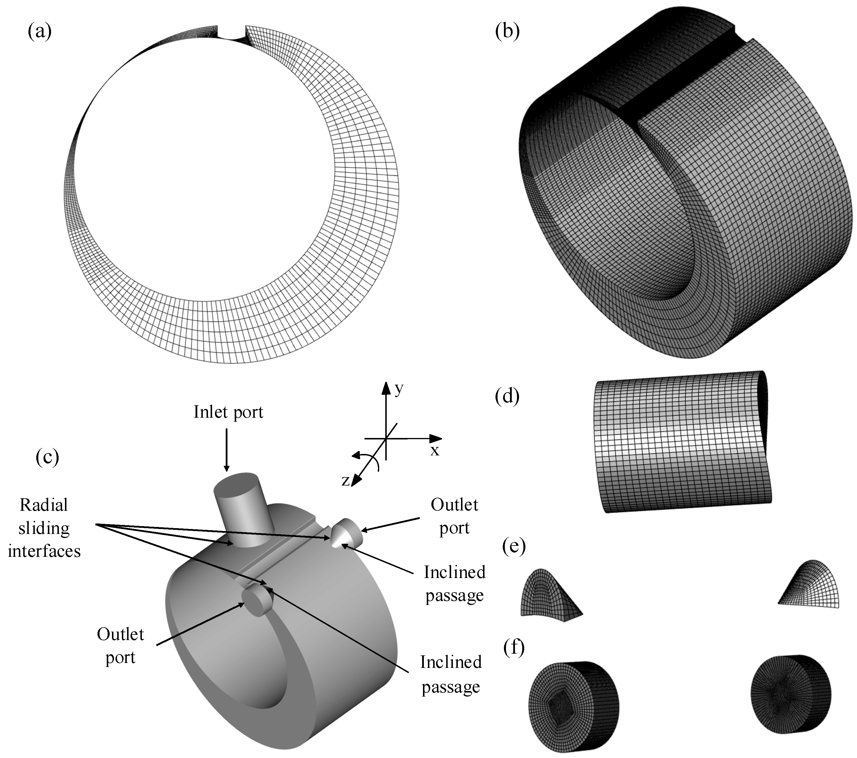
φ 3 _ k , e = π 2 + θ k π 4
The start angles φ 3 _ k , b on the inner boundary are determined recursively from the adjacent subregions
φ 3 _ k , b = φ 2 , e , k = 0   o r   θ k π 4 φ 2 , e φ 3 _ k 1 , e , k 1   a n d   θ k π 4 < φ 2 , e
The start angle α 3 _ k , b and the end angle α 3 _ k , e on the outer boundary are then given by
α 3 _ k , b = π 2 α t , k = 0   o r   θ k π 4 φ 2 , e α 3 _ k , e , k 1   a n d   θ k π 4 < φ 2 , e
α 3 _ k , e = atan 2 y c + R 2 sin φ 3 _ k , e ,   x c + R 2 cos φ 3 _ k , e
For the arc-sector subregions, such as Z o n e   3 _ k , Z o n e   M and Z o n e   4 _ k , the coordinates of the corresponding end points are written in the unified form
x q , s o u t = R 1 cos α q , s , y q , s o u t = R 1 sin α q , s , x q , s i n = x c + R 2 cos φ q , s , y q , s i n = y c + R 2 sin φ q , s , s { b , e } .
where x q , s o u t , y q , s o u t is the coordinate of the end point of region q on the outer boundary; x q , s i n , y q , s i n is the coordinate of the end point of region q on the inner boundary; and s b , e indicates either the start or the end point.

Appendix A.4. Zone M

Z o n e   M connects Z o n e   3 and Z o n e   4 , and its start angle φ M , b and end angle φ M , e are determined from the relative positions of the instantaneous rotor rotation angle θ and the boundary angles associated with the two sides of the vane.
φ M , b = φ 3 _ 4 , e , θ π < φ 2 , e φ 2 , e , θ π φ 2 , e
φ M , e = φ 0 , b 2 π , θ < φ 0 , e θ 2 π , θ φ 0 , e
where φ 3 _ 4 , e is the end angle of Z o n e   3 _ 4 on the inner boundary; φ 2 , e is the end angle of Z o n e   2 on the inner boundary; φ 0 , b is the start angle of Z o n e   0 on the inner boundary; φ 0 , e is the end angle of Z o n e   0 on the inner boundary.
The start angle α M , b and end angle α M , e on the outer boundary are then obtained from
α M , b = α 3 _ 4 , e , θ π < φ 2 , e π 2 α t , θ π φ 2 , e
α M , e = α 0 , b 2 π , θ < φ 0 , e atan 2 y c + R 2 sin θ ,   x c + R 2 cos θ , θ φ 0 , e
where α 3 _ 4 , e is the end angle of Z o n e   3 _ 4 on the outer boundary; α 0 , b is the start angle of the outer boundary of Z o n e   0 . The coordinates of its end points are calculated using Equation (A11).

Appendix A.5. Zone 4_k

Z o n e   4 _ k comprises the main fan-shaped sector on the left side of the vane. Starting from the terminal boundary of Z o n e   M , it is subdivided sequentially in the clockwise direction into up to five candidate subregions ( k = 0 , 1 , , 4 ), extending toward the left endpoint of the vane slot. The initial angles of the inner and outer boundaries ( φ 4 _ k , b and α 4 _ k , b ) of each subregion are inherited from the terminal angles of the adjacent region:
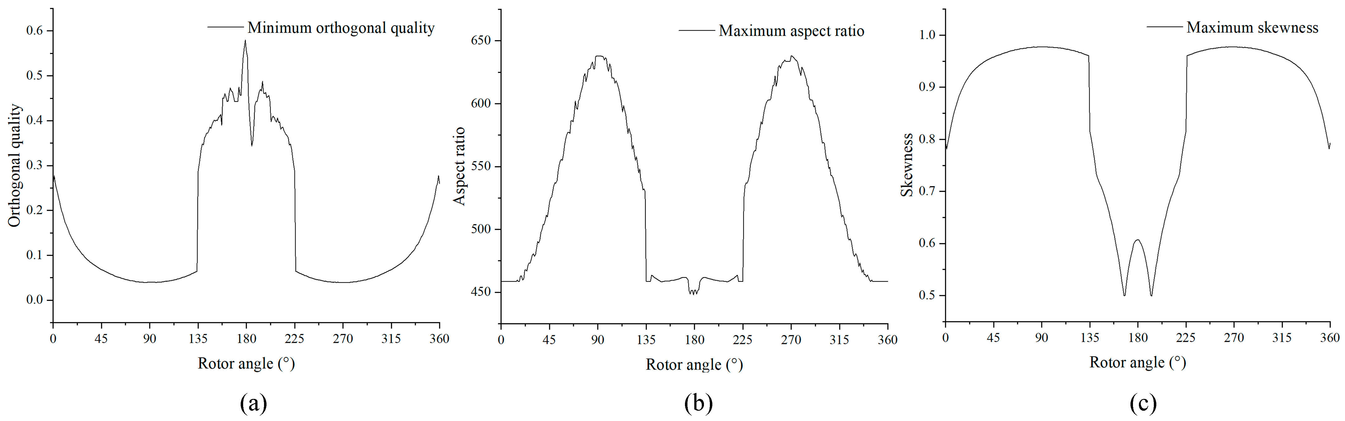
φ 4 _ k , b = φ M , e , k = 0 φ 4 _ k 1 , e , k 1 , α 4 _ k , b = α M , e , k = 0 α 4 _ k 1 , e , k 1
For k = 0 , 1 , 2 , 3 , the candidate rotor rotation angle ψ k associated with the terminal boundary of Z o n e   4 _ k is defined as
ψ k = θ ( k + 1 ) π 4
Z o n e   4 _ k terminates at the next reference ray φ 3 _ k + 1 , e .
When ψ k φ 0 , b , the inner boundary of Z o n e   4 _ k terminates at the candidate point on the rotor outer surface:
φ 4 _ k , e = ψ k 2 π
The corresponding terminal angle on the cylinder inner wall is determined from the intersection between the radial line and the cylinder surface:
α 4 _ k , e = atan 2 y c + R 2 sin ψ k ,   x c + R 2 cos ψ k
The left endpoint of the vane slot lies in the second quadrant and is represented by the outer-boundary angle α 0 , b 2 π . However, the a t a n 2 function in Equation (A19) may return an angle in the interval ( π / 2 , π ] for points in the left-hand quadrant. To maintain angular continuity with α 0 , b 2 π , the computed angle is therefore normalized as
α 4 _ k , e = α o 4 _ k , e 2 π , α 4 _ k , e > π 2
When ψ k < φ 0 , b , the candidate rotor rotation angle has not yet reached the left endpoint of the vane slot. Z o n e   4 _ k is then truncated by the vane, and its terminal boundaries are assigned directly to the left endpoint of the vane slot:
φ 4 _ k , e = φ 0 , b 2 π , α 4 _ k , e = α 0 , b 2 π
Z o n e   4 _ 4 serves as a residual subregion that accommodates the remaining sector between the terminal boundary of Z o n e   4 _ 3 and the left endpoint of the vane slot. Once activated, it therefore terminates directly at the left endpoint of the vane slot:
φ 4 _ 4 , e = φ 0 , b 2 π , α 4 _ 4 , e = α 0 , b 2 π
Accordingly, the terminal angles of the inner and outer boundaries of Z o n e   4 _ k for k = 0,1 , 2,3 can be written in a unified form as
φ 4 _ k , e = ψ k 2 π , ψ k φ 0 , b , φ 0 , b 2 π , ψ k < φ 0 , b ,
α 4 _ k , e = atan 2 y c + R 2 sin ψ k , x c + R 2 cos ψ k , ψ k φ 0 , b , α 0 , b 2 π , ψ k < φ 0 , b .
Any Z o n e   4 _ k that fails the independent-existence criterion, i.e., whose angular extent is below the prescribed minimum, is merged into the adjacent subregion rather than being generated independently. This treatment prevents the formation of excessively narrow regions and ensures a continuous, topologically consistent mesh throughout the rotor rotation cycle.

Appendix B. Node Coordinate Generation

Appendix B.1. Outer-Boundary Nodes

Let the j-th outer-boundary node of region q be r q , j o u t = x q , j o u t , y q , j o u t , where r denotes the position vector of a boundary point or node. For the arc regions ( Z o n e   1 , Z o n e   3 _ k , Z o n e   M and Z o n e   4 _ k ), let the corresponding arc center be x q c , y q c and the radius be ρ q ; the boundary nodes are then distributed at equal angular intervals:
x q , j o u t = x q c + ρ q cos α q , b + j α q , e α q , b n q , y q , j o u t = y q c + ρ q sin α q , b + j α q , e α q , b n q , j = 1 , 2 , , n q .
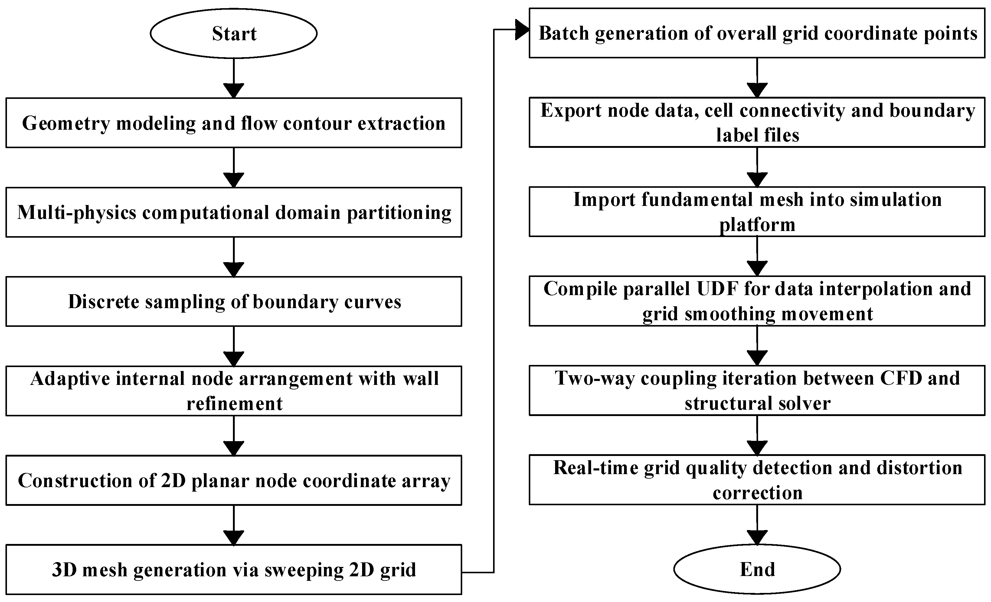
For the straight transition regions ( Z o n e   0 and ( Z o n e   2 ), the boundary nodes are distributed by linear interpolation:
r q , j o u t = r q , b o u t + j n q r q , e o u t r q , b o u t , q { 0 , 2 } , j = 1 , 2 , , n q .
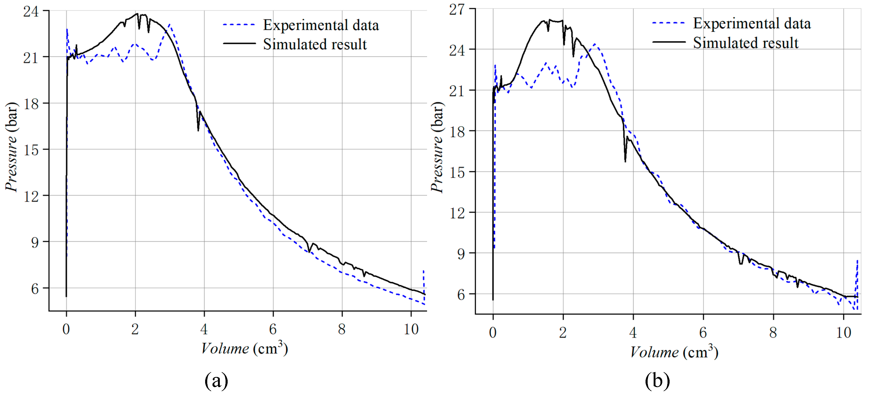
where r q , b o u t = x q , b o u t , y q , b o u t is the coordinate of the start point of region q on the outer boundary; r q , e o u t = x q , e o u t , y q , e o u t is the coordinate of the end point of region q on the outer boundary.

Appendix B.2. Inner-Boundary Nodes

The inner-boundary nodes lie on the rotor outer wall. Let the j-th inner-boundary node of region q be r q , j i n = x q , j i n , y q , j i n ; it is calculated as
x q , j i n = x c + R 2 cos φ q , b + j φ q , e φ q , b n q , y q , j i n = y c + R 2 sin φ q , b + j φ q , e φ q , b n q , j = 1 , 2 , , n q .
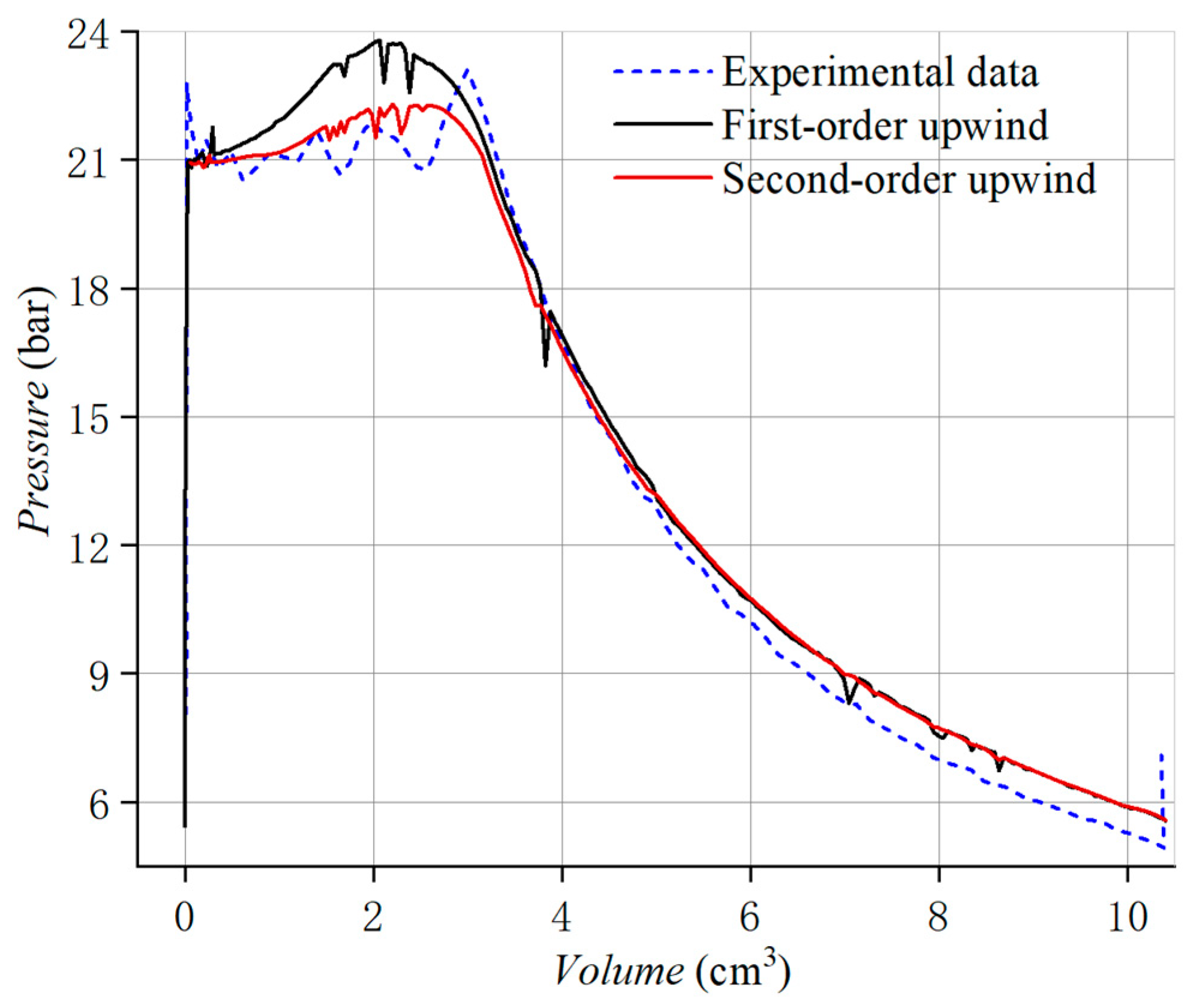
where φ q , b   a n d   φ q , e are the start and end angles of region q on the inner boundary respectively; and n q is the circumferential node number of region q . After the nodes of all regions are assembled in circumferential order, a one-to-one correspondence between the inner and outer-boundary nodes r j o u t , r j i n is established. The line segments connecting boundary-node pairs with the same index form the basis of the radial grid lines.

Appendix B.3. Radial Interior Nodes

Let the number of radial node layers be n r ; the dimensionless radial coordinate of the k -th layer is defined as
λ k = k 1 n r 1 , k = 1 , 2 , , n r
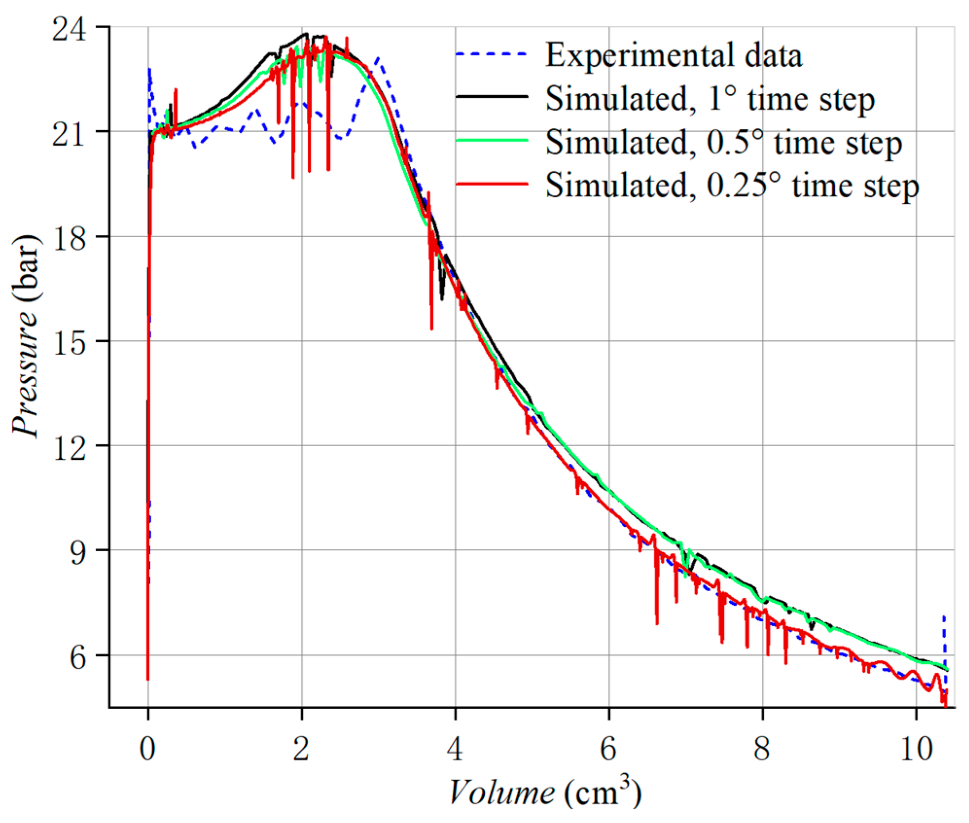
where λ k is the dimensionless radial coordinate of the k -th layer, with λ k = 0 corresponding to the inner boundary and λ k = 1 to the outer boundary. The coordinates of the node on the j -th radial grid line and the k -th radial layer r j , k are then obtained from
r j , k = ( 1 λ k ) r j i n + λ k r j o u t
where r j i n is the coordinate of the j -th inner-boundary node; and r j o u t is the coordinate of the j -th outer-boundary node.
Here, k = 1 corresponds to the inner boundary, k = n r to the outer boundary and k = 2 , 3 , , n r 1 to the interior nodes. This algebraic interpolation preserves the one-to-one correspondence between the inner- and outer-boundary nodes and produces topologically consistent radial grid lines. Figure A1 illustrates the local grids in the vane tip and rotor–cylinder clearance regions at θ = 0 ° and θ   =   180 ° together with the refined grid at the rotor bottom clearance. Figure A1a,b demonstrate that Z o n e   0 2 maintains a regular grid topology despite substantial changes in the effective vane length, while Figure A1c shows that sufficient circumferential resolution is maintained in the rotor-bottom clearance through the adaptive node assignment of Z o n e   3 _ 1 3 _ 4 .
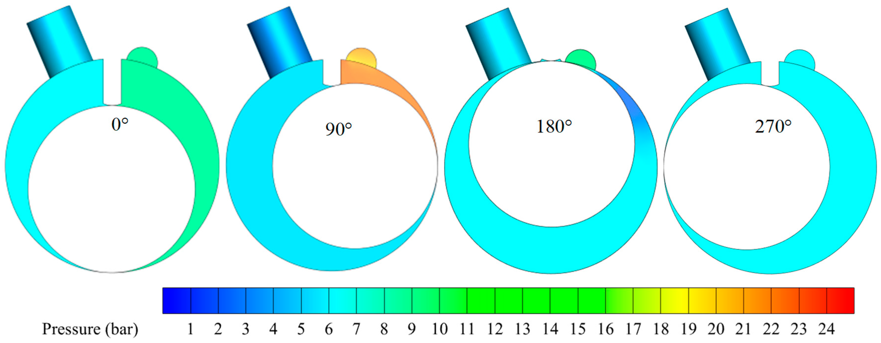
Figure A1. Local grid structures in the clearance regions. (a) Local grid in the vane-tip clearance ( θ = 0 ° ); (b) local grid in the vane-tip clearance ( θ   =   180 ° ) ; (c) refined grid in the rotor–cylinder clearance.
Machines 14 01071 g0a1

Appendix B.4. Axial Extrusion

Let the axial extent of the compressor be z m i n ,   z m a x   and let the number of axial node layers be n a ; the coordinate of the m -th axial plane z m is given by
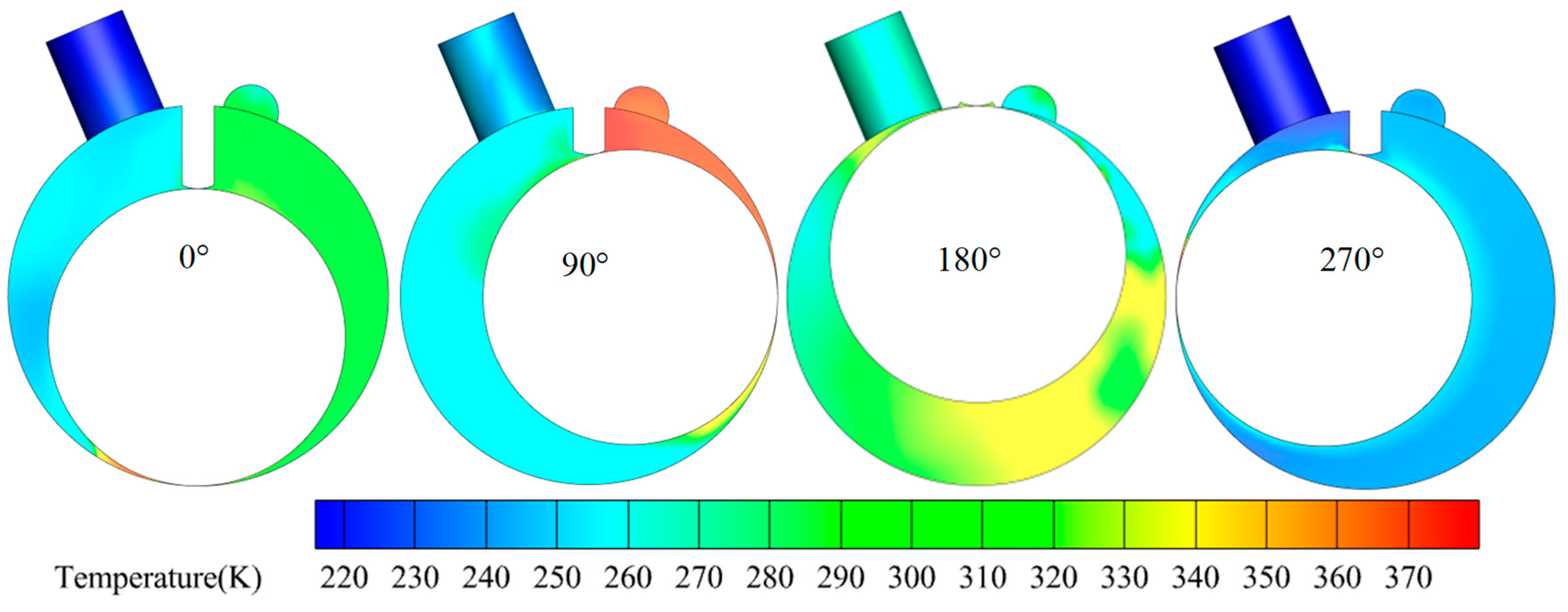
z m = z max + ( m 1 ) z max z min n a 1 , m = 1 , 2 , , n a .
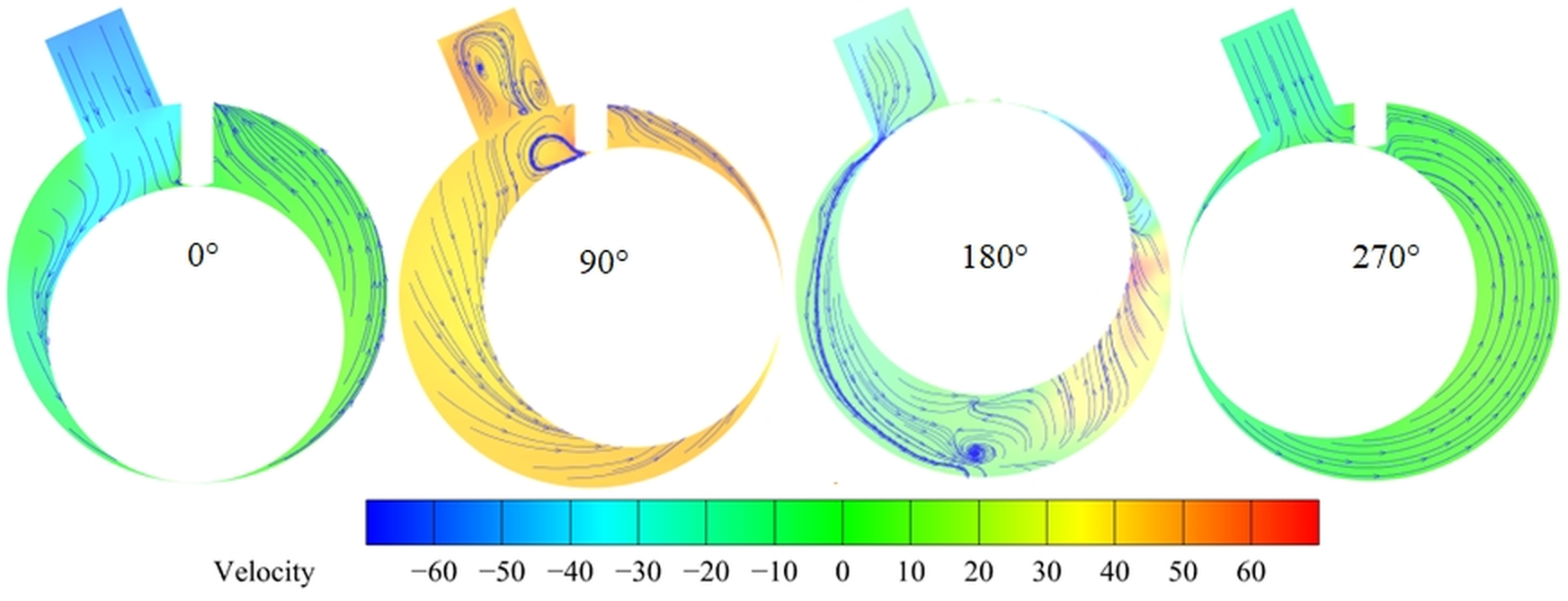
The two-dimensional node coordinates of each layer are then replicated onto the corresponding z m planes to construct the three-dimensional structured grid, whose total node number is
n t = n c n r n a

References

  1. Aw, K.T.; Ooi, K.T. A Review on Sliding Vane and Rolling Piston Compressors. Machines 2021, 9, 125. [Google Scholar] [CrossRef] [Scilit]
  2. Wu, J.; Lin, J.; Zhang, Z.; Chen, Z.; Xie, J.; Lu, J. Experimental Investigation of Dynamic Characteristics of a Rotary Compressor and Its Air Conditioner Using R290 during Warm Startup. Appl. Therm. Eng. 2017, 125, 1469–1477. [Google Scholar] [CrossRef] [Scilit]
  3. Ooi, K.T. Design Optimization of a Rolling Piston Compressor for Refrigerators. Appl. Therm. Eng. 2005, 25, 813–829. [Google Scholar] [CrossRef] [Scilit]
  4. Vega Benavente, J.I.; Gendebien, S.; Lemort, V. Experimental Study and Modelling of a 2-Stage Compression R744 Refrigeration System with Vapor Injection and Inter-Cooling. In Proceedings of the 19th International Refrigeration and Air Conditioning Conference at Purdue, West Lafayette, IN, USA, 10–14 July 2022; Purdue University: West Lafayette, IN, USA, 2022; p. 2546. [Google Scholar]
  5. Wen, C.; Bai, P.; Zhang, H.; Zhang, S.; Meng, X.; Meng, Y.; Tian, Y. Theoretical Model Development and Mixed Lubrication Analyses of Rolling Piston Type Rotary Compressors: A Review. Lubricants 2024, 12, 273. [Google Scholar] [CrossRef] [Scilit]
  6. Zheng, C.; Zhao, W.; Lyu, B.; Gao, K.; Cao, H.; Zhong, L.; Gao, Y.; Liao, R. Performance Analysis for a Rotary Compressor at High Speed: Experimental Study and Mathematical Modeling. Appl. Therm. Eng. 2025, 263, 125275. [Google Scholar] [CrossRef] [Scilit]
  7. Yang, J.; Qi, Z.; Chen, J.; Chen, Z. Experimental Study on a Two-Stage Rolling Piston CO2 Compressor Based on p–V Indicator Diagrams. Proc. Inst. Mech. Eng. Part C J. Mech. Eng. Sci. 2012, 226, 995–1003. [Google Scholar] [CrossRef] [Scilit]
  8. Wu, J.; Wang, G.; Li, Y.; Chen, A.; Gao, Q.; Chen, Z.; Jiang, B. Experimental Study on P–V Diagram and Valve Displacement of a HC290 Rotary Compressor. Proc. Inst. Mech. Eng. Part C J. Mech. Eng. Sci. 2015, 229, 3113–3124. [Google Scholar] [CrossRef] [Scilit]
  9. Patel, B.; Kovacevic, A.; Plantegenet, T.; Tam, T. Study of Leakage Flow in Oil-Free Positive Displacement Rotary Machines Using Particle Image Velocimetry. Exp. Therm. Fluid Sci. 2023, 145, 110886. [Google Scholar] [CrossRef] [Scilit]
  10. Kovacevic, A.; Stosic, N.; Smith, I.K. Screw Compressors: Three Dimensional Computational Fluid Dynamics and Solid Fluid Interaction; Springer: Berlin/Heidelberg, Germany, 2007. [Google Scholar]
  11. Karpenko, M. Aircraft Hydraulic Drive Energy Losses and Operation Delay Associated with the Pipeline and Fitting Connections. Aviation 2024, 28, 1–8. [Google Scholar] [CrossRef] [Scilit]
  12. Karpenko, M.; Stosiak, M.; Šukevičius, Š.; Skačkauskas, P.; Urbanowicz, K.; Deptuła, A. Hydrodynamic Processes in Angular Fitting Connections of a Transport Machine’s Hydraulic Drive. Machines 2023, 11, 355. [Google Scholar] [CrossRef] [Scilit]
  13. Demirdžić, I.; Perić, M. Space Conservation Law in Finite Volume Calculations of Fluid Flow. Int. J. Numer. Methods Fluids 1988, 8, 1037–1050. [Google Scholar] [CrossRef] [Scilit]
  14. Kovacevic, A. Boundary Adaptation in Grid Generation for CFD Analysis of Screw Compressors. Int. J. Numer. Methods Eng. 2005, 64, 401–426. [Google Scholar] [CrossRef] [Scilit]
  15. Utri, M.; Brümmer, A. A Comparative Examination of the Potential of Screw Expanders with Variable Rotor Pitch. In Proceedings of the International Screw Compressor Conference, Dortmund, Germany, 23–24 September 2014. [Google Scholar]
  16. Spille-Kohoff, A.; Hesse, J.; El Shorbagy, A. CFD Simulation of a Screw Compressor Including Leakage Flows and Rotor Heating. IOP Conf. Ser. Mater. Sci. Eng. 2015, 90, 012009. [Google Scholar] [CrossRef] [Scilit]
  17. Hesse, J.; Andres, R. CFD Simulation of a Dry Scroll Vacuum Pump Including Leakage Flows. In Proceedings of the 23rd International Compressor Engineering Conference at Purdue, West Lafayette, IN, USA, 11–14 July 2016; Purdue University: West Lafayette, IN, USA, 2016; p. 1515. [Google Scholar]
  18. Zhang, Q.; Xu, X.Y. Numerical Simulation on Cavitation in a Vane Pump with Moving Mesh. In Proceedings of the 5th International Conference on Computational Methods (ICCM2014), Cambridge, UK, 28–30 July 2014. [Google Scholar]
  19. Montenegro, G.; Della Torre, A.; Fiocco, M.; Onorati, A.; Benatzky, C.; Schlager, G. Evaluating the Performance of a Rotary Vane Expander for Small Scale Organic Rankine Cycles Using CFD Tools. Energy Procedia 2014, 45, 1136–1145. [Google Scholar] [CrossRef] [Scilit]
  20. Kolasiński, P.; Błasiak, P. Numerical and Experimental Investigation on the Rotary Vane Expander Operation in Micro ORC System. In Proceedings of the 3rd International Seminar on ORC Power Systems, Brussels, Belgium, 12–14 October 2015. [Google Scholar]
  21. Bianchi, G.; Rane, S.; Kovacevic, A.; Cipollone, R. Deforming Grid Generation for Numerical Simulations of Fluid Dynamics in Sliding Vane Rotary Machines. Adv. Eng. Softw. 2017, 112, 180–191. [Google Scholar] [CrossRef] [Scilit]
  22. Ye, F.; Bianchi, G.; Rane, S.; Tassou, S.A.; Deng, J. Analytical Grid Generation and Numerical Assessment of Tip Leakage Flows in Sliding Vane Rotary Machines. Adv. Eng. Softw. 2021, 159, 103030. [Google Scholar] [CrossRef] [Scilit]
  23. Gu, H.; Chen, Y.; Wu, J.; Jiang, Y.; Sundén, B. Impact of Discharge Port Configurations on the Performance of Sliding Vane Rotary Compressors with a Rotating Cylinder. Appl. Therm. Eng. 2021, 186, 116526. [Google Scholar] [CrossRef] [Scilit]
  24. Du, Y.; Li, S.; Wu, J.; Liu, Q.; Zhao, Z. Research on the Motion Characteristics of Sliding Vane in Rolling Piston Compressor under Low-Speed Condition. Int. J. Refrig. 2026, 182, 522–532. [Google Scholar] [CrossRef] [Scilit]
  25. Pandeya, P.N.; Soedel, W. Rolling Piston Type Rotary Compressors with Special Attention to Friction and Leakage. In Proceedings of the International Compressor Engineering Conference at Purdue, West Lafayette, IN, USA, 1978; Purdue University: West Lafayette, IN, USA, 1978; p. 268. [Google Scholar]
  26. Zeng, W.; Pan, X.; Chen, J.; Xie, J. Investigation on a R32 Rotary Compressor with Vapor Injection by Supplementary Valve Based on FSI Simulation. Int. J. Refrig. 2026, 181, 215–227. [Google Scholar] [CrossRef] [Scilit]
  27. Farkas, B.; Szente, V.; Suda, J.M. A Simplified Modeling Approach for Rolling Piston Compressors. Period. Polytech. Mech. Eng. 2015, 59, 94–101. [Google Scholar] [CrossRef] [Scilit]
  28. Ding, H.; Gao, H. 3-D Transient CFD Model for a Rolling Piston Compressor with a Dynamic Reed Valve. In Proceedings of the 22nd International Compressor Engineering Conference at Purdue, West Lafayette, IN, USA, 14–17 July 2014; Purdue University: West Lafayette, IN, USA, 2014; p. 1548. [Google Scholar]
  29. Cavazzini, G.; Giacomel, F.; Benato, A.; Nascimben, F.; Ardizzon, G. Analysis of the Inner Fluid-Dynamics of Scroll Compressors and Comparison between CFD Numerical and Modelling Approaches. Energies 2021, 14, 1158. [Google Scholar] [CrossRef] [Scilit]
  30. Basha, N.; Kovacevic, A.; Rane, S. User Defined Nodal Displacement of Numerical Mesh for Analysis of Screw Machines in FLUENT. IOP Conf. Ser. Mater. Sci. Eng. 2019, 604, 012012. [Google Scholar] [CrossRef] [Scilit]
  31. Aungier, R.H. A Fast, Accurate Real Gas Equation of State for Fluid Dynamic Analysis Applications. J. Fluids Eng. 1995, 117, 277–281. [Google Scholar] [CrossRef] [Scilit]
  32. Menter, F.R. Two-Equation Eddy-Viscosity Turbulence Models for Engineering Applications. AIAA J. 1994, 32, 1598–1605. [Google Scholar] [CrossRef] [Scilit] [PubMed]
Figure 1. Flow chart of the analytical grid generation method for CFD simulations of RPCs.
Machines 14 01071 g001
Figure 2. Schematic of the two-dimensional cross-sectional geometry of the RPC.
Machines 14 01071 g002
Figure 3. Geometry of the RPC and enlarged view of vane and slot. (a) Overall geometry: The outer circle represents the cylinder inner wall (cylinder, with center O 1 and radius R 1 ); the inner circle represents the rotor outer wall (rotor, with center O 2 and radius R 2 ); the eccentric distance between the two centers is ε , the rotor radius ratio is κ , the rotor–cylinder radial clearance is δ c , and the vane thickness is d ; (b) enlarged view of vane and slot: ± x t ,   y t is the intersection point between the vane slot and the cylinder inner wall, α t is the angle subtended at the cylinder center O 1 by the left end point of the slot, α is the parametric angle from the cylinder center to the reference point x o u t ,   y o u t on the cylinder inner wall.
Machines 14 01071 g003
Figure 4. Geometric definition and position variation in the rotor profile (inner boundary). (a) Configuration with the rotor at θ   =   0 ° ; (b) configuration after eccentric rotation of the rotor about the cylinder center to the position θ   =   90 ° , showing the inner boundary parametric angle φ and an arbitrary point x i n ,   y i n on the rotor outer wall.
Machines 14 01071 g004
Figure 5. Schematic of the vane geometry and the short-vane correction strategy: (a) normal-vane configuration, with the vane fully protruding, the end point d 2 ,   h l below the slot intersection point x t ,   y t , and the protrusion length L l equal to the straight-line distance between them; (b) short-vane configuration θ     180 ° , with most of the vane retracted into the slot, the end point d 2 ,   h l above the slot intersection point x t ,   y t , the protrusion length smaller than 0.06 R 1 , and the slot intersection point moving outward after the root half-angle correction, which enlarges the mappable angular range.
Machines 14 01071 g005
Figure 6. Boundary splitting of the two-dimensional cross-section and the definition of the start and end angles on the inner and outer boundaries. (a) Overall split, showing the vane region ( Z o n e   1 ), the transition regions ( Z o n e   0 ,   Z o n e   2   a n d   Z o n e   M ) and the core region ( Z o n e   3 _ k ); (b) start and end angles on the outer boundary (cylinder inner wall); (c) start and end angles on the inner boundary (rotor outer wall).
Machines 14 01071 g006
Figure 7. Adaptive adjustment of the main-sector split at different rotor rotation angles. (a) θ   =   0 ° , all five subregions Z o n e   3 _ 0 Z o n e   3 _ 4 of Zone 3 are present; (b) θ   =   90 ° , Z o n e   3 _ 0 has merged away and Z o n e   3 _ 1 Z o n e   3 _ 4 are retained; (c) θ   =   180 ° , only Z o n e   3 _ 3 and Z o n e   3 _ 4 remain on the right side of the vane while Z o n e   4 _ 0 and Z o n e   4 _ 1 begin to form on the left; (d) θ   =   270 ° , the Z o n e   3 candidate subregions have completely merged and the Z o n e   4 candidate subregions are fully developed on the left side.
Machines 14 01071 g007
Figure 8. Critical intervals for the transition between Z o n e s   3   a n d   4 . The dashed lines denote the reference rays φ 3 _ k , e = θ + ( 2 k ) π / 4 ( k = 0 , , 4 ), which rotate rigidly with the rotor. (ac) First transition: (a) θ   =   80 ° , all five subregions of Z o n e 3 are present; (b) θ   =   100 ° , Z o n e 3 _ 0 has been removed and absorbed into Z o n e 3 _ 1 ; (c) θ   =   115 ° , Z o n e   4 _ 0 begins to form. (df) Final transition: (d) θ   =   240 ° , only Z o n e 3 _ 4 remains; (e) θ   =   262 ° , the gap is bridged by Z o n e M ; (f) θ   =   290 ° , the Z o n e   4 candidate subregions are complete.
Machines 14 01071 g008
Figure 9. Mesh distributions at different rotational angles.
Machines 14 01071 g009
Figure 10. CFD model of the RPC: (a) 2D rotor mesh; (b) 3D rotor mesh; (c) assembled model, (d) inlet port mesh; (e) inclined passage mesh; (f) outlet port mesh.
Machines 14 01071 g010
Figure 11. Variation in rotor-region mesh quality metrics with rotor angle: (a) minimum orthogonal quality; (b) maximum aspect ratio; (c) maximum skewness.
Machines 14 01071 g011
Figure 12. Flow chart for analytical grid generation coupling with CFD solvers.
Machines 14 01071 g012
Figure 13. Comparison of simulated and experimental p–V diagrams at different rotational speeds: (a) 80 Hz; (b) 120 Hz.
Machines 14 01071 g013
Figure 14. Comparison of experimental and simulated p–V diagrams using first- and second-order upwind schemes at 80 Hz.
Machines 14 01071 g014
Figure 15. Comparison of experimental and simulated p V diagrams with different angular time steps at 80 Hz.
Machines 14 01071 g015
Figure 16. Pressure contours in the compression chamber at different rotor rotation angles.
Machines 14 01071 g016
Figure 17. Temperature contours in the compression chamber at different rotor rotation angles.
Machines 14 01071 g017
Figure 18. Velocity contours and streamlines in the compression chamber at different rotor rotation angles.
Machines 14 01071 g018
Table 1. Geometric parameters and number of negative-volume cells for different test cases.
Case κ ε (m) r v (m)Number of Negative-Volume Cells
Case 00.78040.004490.00410
Case 10.74000.005320.00410
Case 20.78040.004490.00300
Case 30.78040.004300.00410
Table 2. Qualitative comparison of dynamic mesh strategies and the proposed analytical grid-generation method.
Comparison CriterionConventional Solver-Based Dynamic Mesh MethodsProposed Analytical Grid-Generation Method
Grid generationUpdated during the CFD solution processPrecomputed outside the CFD solver
Solver dependencyRelies on built-in dynamic mesh, smoothing, or remeshing functionsLess dependent on solver-side mesh-processing functions
Grid topologyLocal reconstruction or topology changes may occur under large deformationPreserves the predefined grid connectivity under a fixed working-chamber topology
Nodal motionControlled by smoothing algorithms and reconstruction criteriaDirectly determined by analytical geometric relationships
Convergence behaviorGrid reconstruction may introduce local convergence disturbancesAvoids repeated grid reconstruction and reduces disturbances associated with mesh updates
Numerical stabilityReconstruction failure, negative-volume cells, or local grid degradation may occurAvoids remeshing failure, although local grid quality may still vary with rotor position
Numerical errorInfluenced by grid resolution, grid quality, and discretization schemesDoes not directly reduce discretization error and remains affected by grid resolution, time-step size, and discretization schemes
Computational costAdditional mesh-smoothing or reconstruction operations are required during the solutionGrid coordinates are generated in advance, reducing solver-side mesh-update calculations
PreprocessingInitial setup is relatively straightforward, but dynamic mesh parameters may require adjustmentRequires initial construction of the analytical mapping; once established, grids for the complete cycle can be generated automatically
Geometric adaptabilityMore flexible for complex or non-prescribed motionsSuitable for RPCs with well-defined motion and unchanged working-chamber topology
Main limitationSensitive to dynamic mesh parameters and grid-quality criteriaRelies on predefined analytical relationships; topology changes require reconstruction of the mapping framework
Table 3. Geometric parameters of the RPC.
QuantitiesValuesUnits
Cylinder radius/R10.0205m
Rotor radius/R20.016m
Eccentricity/ε0.0045m
Axial length/Z0.022m
Vane thickness/d0.00345m
Radius of vane-tip arc/rv0.0041m
Clearance between rotor and cylinder/δc0.00001m
Clearance between vane and rotor/δv0.00001m
Suction port angle203°
Discharge port angle164°
Table 4. Mesh quality of inlet and outlet ports.
Mesh QualityInlet PortOutlet PortInclined Passage
Maximum aspect ratio5.7533.8036.562
Maximum expansion factor2.8182.6757.786
Minimum orthogonality0.7580.7770.486
Maximum skewness0.5160.5310.318
Total cell count28,00025,0803555
Table 5. Comparison of preprocessing efficiency between the conventional mesh generation method and the proposed analytical grid generation method.
Comparison ItemConventional Mesh Generation MethodProposed Analytical Grid Generation Method
Geometric modelSame rolling-piston compressor geometrySame rolling-piston compressor geometry
Rotation cycle0–360°0–360°
Number of rotor positions360360
Total number of mesh configurations360 mesh configurationsNodal positions corresponding to 360 rotor positions
Mesh generation approachMeshes generated separately at each rotor position using conventional preprocessing softwareNodal displacements automatically computed from analytical expressions
SoftwareANSYS ICEM CFD 2022R1MATLAB R2021a
CPUAMD Ryzen 9 7950X 16-Core ProcessorAMD Ryzen 9 7950X 16-Core Processor
Memory64 GB64 GB
Level of manual interventionHigh; repeated mesh generation, quality inspection, and local adjustment are required when necessaryLow; nodal positions at different rotor angles are generated automatically after the initial parameters are specified
Mesh generation required at each rotor positionYesNo
CFD solution time includedNoNo
Preprocessing timeApproximately 48 hApproximately 54 s
Reduction in preprocessing timeApproximately 99.97%
Definition of preprocessing timeCumulative preprocessing time required to generate the dynamic meshes over one complete revolutionTime required to generate nodal coordinates/mesh displacements over one complete revolution
Table 6. Detailed settings in ANSYS Fluent 2022R1 solver.
CriteriaItemSetting or Value
Solver typeSolver TypePressure-Based Solver
Physical propertiesR32Aungier–Redlich–Kwong real-gas model
Turbulence ModelTurbulence ModelSST k–ω
Pressure–Velocity CouplingCoupled
GradientLeast Squares Cell Based
Solution MethodsPressure DiscretizationStandard
Density DiscretizationFirst-Order Upwind
Momentum DiscretizationFirst-Order Upwind
Turbulent Kinetic Energy DiscretizationFirst-Order Upwind
Specific Dissipation Rate DiscretizationFirst-Order Upwind
Energy DiscretizationFirst-Order Upwind
Transient FormulationTransient FormulationFirst-Order Implicit
Flow Courant Number2
Explicit Relaxation Factor0.5
Under-Relaxation Factor0.2
Convergence criterionContinuity, momentum, k, and ω0.001
Energy0.000001
Solution ControlsConvergence Criterion0.001
Angular Step Size
Number of Time Steps360
Maximum Iterations per Time Step50
Table 7. Comparison of experimental and numerical conditions used for model validation.
CategoryParameterExperimentPresent SimulationMeasurement Uncertainty
GeometryCylinder inner-wall radius, R 1 (m)0.02050.0205
Rotor radius, R 2 (m)0.0160.0159982
Eccentricity, ε (m)0.00450.0044918
Working fluidRefrigerantR32R32
80 Hz conditionSuction pressure (bar)5.05.0
Discharge pressure (bar)21.021.0±0.05
Suction temperature (K)267.15267.15±0.05
Rotational speed (rpm)48004800±0.02
120 Hz conditionSuction pressure (bar)5.05.0
Discharge pressure (bar)21.021.0±0.05
Suction temperature (K)267.15267.15±0.05
Rotational speed (rpm)72007200±0.02
Table 8. Grid independence analysis with radial grid refinement.
ItemCoarse MeshMedium MeshFine Mesh
Cell count of rotor domain122,615173,601231,655
Number of radial cells4712
Number of axial cells303030
Discharge temperature310.814308.975308.569
Absolute relative difference in discharge temperature (%)-0.5950.132
Table 9. Grid independence analysis with axial grid refinement.
ItemCoarse MeshMedium MeshFine Mesh
Cell count of rotor domain135,303173,601205,805
Number of radial cells777
Number of axial cells203045
Discharge temperature310.763308.975308.682
Absolute relative difference in discharge temperature (%)-0.5790.095
Table 10. GCI analysis of grid discretization uncertainty.
Grid Refinement Directionr32r21Apparent Order of ConvergenceExtrapolated Temperature (K)GCI32 (%)GCI21 (%)
Radial1.7501.7142.670308.4430.2150.051
Axial1.5001.5004.461308.6250.1420.023
Disclaimer/Publisher’s Note: The statements, opinions and data contained in all publications are solely those of the individual author(s) and contributor(s) and not of MDPI and/or the editor(s). MDPI and/or the editor(s) disclaim responsibility for any injury to people or property resulting from any ideas, methods, instructions or products referred to in the content.