Article

Auxiliary Energy Consumption Characteristics and Prediction Models for Range-Extended Electric Vehicles

1
China Automotive Technology and Research Center Co., Ltd., Tianjin 300300, China
2
CATARC Automotive Test Center (Tianjin) Co., Ltd., Tianjin 300300, China
3
Tianjin Key Laboratory of Power Transmission and Safety Technology for New Energy Vehicles, Hebei University of Technology, Tianjin 300401, China
*
Authors to whom correspondence should be addressed.
Machines 2026, 14(9), 1043; https://doi.org/10.3390/machines14091043
Submission received: 18 August 2026 / Revised: 9 September 2026 / Accepted: 11 September 2026 / Published: 14 September 2026
(This article belongs to the Special Issue Intelligent Control and Optimization of Green and Clean Powertrains)

Abstract

Auxiliary energy consumption rises sharply at low temperatures, reducing the accuracy of driving range prediction and vehicle energy management. Most previous studies have focused on battery electric vehicles, whose operating characteristics do not fully represent the powertrain architecture of range-extended electric vehicles (REEVs). This study analyzes REEV auxiliary energy consumption and develops prediction models for operation at low temperatures. Approximately 3600 km of actual road driving data were collected. Auxiliary energy consumption was examined across four dimensions: power mode, trip scale, thermal management load, and range-extender operating share. Engine waste heat reduced auxiliary energy consumption by more than 59% in range-extended mode compared with pure-electric mode. Random Forest (RF), Least-Squares Boosting (LSBoost), and Multilayer Perceptron (MLP) methods were used to develop a trip-scale auxiliary energy consumption prediction model (trip-scale model) and a second-scale auxiliary energy consumption prediction model (second-scale model). The best test-set R2 was 0.826 for the trip-scale model. For the second-scale model, R2 increased from 0.857 at 30 s to a maximum of 0.872 at 60 s; considering that doubling the sample duration yielded an R2 improvement of only 0.015, the 30 s LSBoost model was selected for subsequent integrated prediction. In the integrated application, the selected model predicted the mean auxiliary power over the remaining trip to estimate the remaining auxiliary energy. Although the departure estimate had a 9.55% error, iterative updates kept the entire estimate close to the measured value, with a maximum absolute residual of 0.022 kWh.

1. Introduction

Transport is a major target for energy conservation and carbon emission reduction during the global energy transition. Conventional vehicles still experience deterioration in NOx emissions, pollutant formation during combustion, and variations in combustion efficiency under real-world operation [1,2,3]. These problems highlight the need to control transport energy use and pollutant emissions together. The International Energy Agency reports that transport accounts for more than 25% of global final energy use. The sector depends on fossil fuels for more than 90% of its energy and produces about 24% of energy-related carbon dioxide emissions [4]. Countries have therefore introduced stricter policies to accelerate powertrain transformation [5]. Electrified vehicles offer efficient energy conversion and near-zero tailpipe emissions during use [6,7]. However, their energy consumption varies greatly in complex real-world conditions. The increase at low temperatures remains a major barrier to energy efficiency and user experience.
Accurate energy prediction requires appropriate prediction algorithms and their effective implementation, which together support real-time vehicle energy management, trip planning, and onboard control [8]. Existing methods are broadly classified as physics-based or data-based. Physics-based studies combine vehicle dynamics with component characteristics. Genikomsakis et al. [9] included powertrain efficiency and regenerative braking and achieved a cumulative energy mean absolute error (MAE) below 45 Wh in standard cycles. Gallet et al. [10] combined longitudinal dynamics with low-resolution operational data for a large bus network and found that approximately 50% of the routes in Singapore required less than 40 kWh per trip. Beckers et al. [11] developed an electric city bus model. Vehicle tests showed that it tracked cumulative energy well, although road grade affected the prediction. These models are physically interpretable but depend strongly on vehicle parameters and boundary conditions. Data-based methods reduce this dependence. Abdelaty et al. [12] used multiple regression to examine road class, passenger load, and air conditioning operation. Their entire trip predictions exceeded 90% accuracy. Zhang et al. [13] combined real-world data with driving condition prediction and obtained a root mean square error (RMSE) of 0.159 kWh and a mean absolute percentage error (MAPE) of 12.68%. Qin et al. [14] optimized support vector regression with the grey wolf algorithm and reported a MAPE of 14.47% for electric bus trips. Nan et al. [15] combined long short-term memory and convolutional neural networks and achieved an R2 of 0.814. Their model remained stable across temperature ranges and complex scenarios. These studies advanced vehicle energy prediction but most targeted total or driving energy consumption and did not fully consider auxiliary consumption.
Vehicle energy consumption comprises driving energy consumption and auxiliary energy consumption, and accurate prediction must include both components. Auxiliary loads include cabin climate control, traction battery thermal management, controllers, pumps, fans, and onboard electrical equipment [16,17]. Cabin and battery heating demands increase at low temperatures. Continuous operation of the thermal management system then increases the contribution of auxiliary energy consumption [18]. Ramesh et al. [19] reported that auxiliary consumption increased more than fivefold when ambient temperature fell from 10 °C to −20 °C. Driving energy consumption mainly follows vehicle dynamics, whereas auxiliary energy consumption also depends on trip duration, battery thermal state, thermal management load, and control strategy. Schäfers et al. [20] showed that omitting auxiliary loads reduces the reliability of vehicle energy demand estimates. Auxiliary energy consumption must therefore be separated from total consumption and modeled according to its own operating characteristics.
Previous auxiliary energy consumption models have important limitations. Valentina et al. [21] developed a thermodynamic model for heating, ventilation, and air conditioning (HVAC), but it required detailed component parameters and extensive calibration for each vehicle. De Cauwer et al. [22] represented auxiliary use with a linear term in a total energy model but did not predict auxiliary energy consumption directly. Kim et al. [23] used several machine learning methods for battery electric vehicles and achieved a prediction accuracy of 0.906, but their model cannot be transferred directly to an REEV. An REEV can draw energy from both the traction battery and the range-extender generator. Its auxiliary loads at low temperatures therefore differ from those of a battery electric vehicle. In pure-electric mode, electrical thermal management components provide cabin and battery heating. When the range-extender operates, engine heat can enter the coolant loop and support both functions [24,25]. This heat changes the load allocation among the positive temperature coefficient (PTC) heater, compressor, and other components. Activation time, coolant thermal state, and thermal management demand may jointly affect auxiliary consumption. No previous study has examined these effects for an REEV during real-world driving at low temperatures.
To address these limitations, this study investigates the characteristics and prediction of REEV auxiliary energy consumption in actual user travel scenarios. A trip-scale model is developed to estimate auxiliary energy consumption for the entire trip, while a second-scale model updates the prediction during driving and supports iterative estimation of the remaining auxiliary energy consumption. The two models are integrated across their respective time scales. The principal innovations are as follows:
(1)
an auxiliary energy prediction framework is established for low-temperature REEV operation by considering range-extender participation and waste heat utilization;
(2)
trip-scale initialization is coupled with second-scale state aggregation to update the predicted remaining auxiliary energy during driving, linking initial trip estimation with online energy management.
The proposed framework can support the development of auxiliary energy prediction systems for REEVs and provide methodological guidance for improving vehicle energy management under low-temperature conditions.

2. Data and Methods

2.1. Vehicle Auxiliary Energy Consumption Data Collection

A Li Auto L8 REEV was selected as the test vehicle, and data collection tests were conducted in Wuhan, China, in January 2026. The detailed vehicle specifications are presented in Table 1. To represent real-world travel scenarios, the test route covered urban, suburban, expressway, and mountainous roads. A closed-loop route was used to reduce the influence of differences between the starting and ending locations on comparisons among operating conditions. The tests covered forced pure-electric and range-extended modes, as well as ECO and SPORT driving modes. Regenerative braking was maintained at the standard setting to minimize interference from differences in control strategy. Tests in pure-electric mode preferentially began at a relatively high state of charge (SOC). When battery charge became insufficient, the vehicle switched modes according to its production control strategy to ensure continuity of road testing.
According to concurrent meteorological observations in Wuhan, the mean ambient temperature during the tests was approximately 1.2 °C. Cabin heating was activated throughout the low-temperature tests following the procedure specified in GB/T 18386.1-2021 [28]. The automatic HVAC system was initially set to 22 °C, and after the cabin temperature reached 20 °C, the temperature setting was adjusted to maintain the average cabin temperature within 20–22 °C. This condition is representative of a typical low-temperature winter travel scenario for local vehicle users. Under these conditions, cabin heating and traction battery thermal management were generally active. During range-extender operation, waste heat generated by the engine can be transferred through the thermal management circuit to support cabin and battery heating, thereby affecting auxiliary energy consumption. The data collection tests covered the complete process from the generation to the effective use of engine waste heat and thus provided a reliable basis for the subsequent analysis.
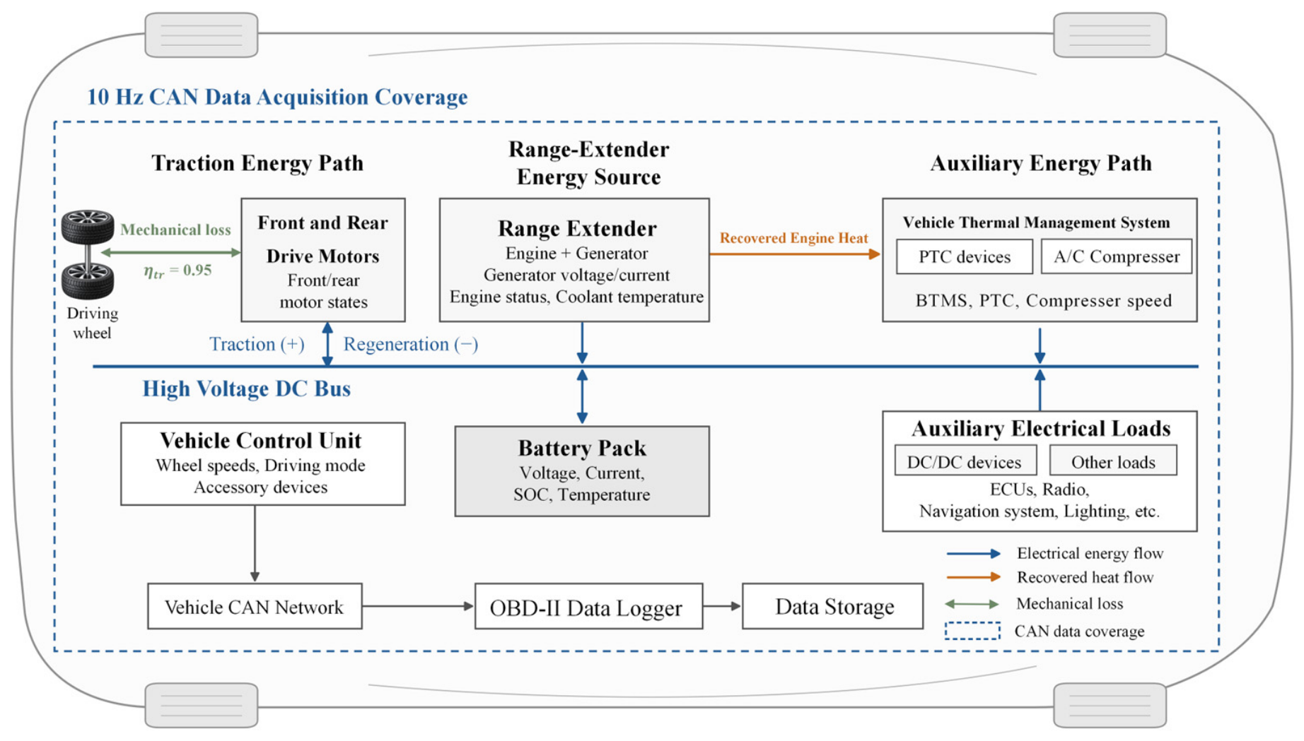
Vehicle operating data were collected using an in-house China driving cycle data acquisition terminal, while an energy-flow acquisition system measured the voltage and current of low-voltage auxiliary components [29]. The acquisition architecture is shown in Figure 1. The driving cycle terminal accessed the controller area network (CAN) through the onboard diagnostics II (OBD-II) interface and read raw signals from the electronic control units (ECUs) in real time. It required no modification of the vehicle electrical circuits and provided stable acquisition, high signal fidelity, and reliable time synchronization during long-duration, high-frequency testing on complex roads at low temperatures. The energy-flow system used high-precision fuse-type current sensors installed in series at the fuses in the vehicle distribution box. This arrangement enabled nondestructive acquisition of wiring harness signals while preserving the original harness. CreaSens SHUNT-CAN sensors were used, with a maximum range of 60 A and a stated accuracy of ±0.01% full scale (F.S.), enabling current measurements at the milliampere level. The recorded parameters covered vehicle operation, vehicle battery state, range-extender operation, the traction system, and the thermal management system. Representative signals included wheel speed, acceleration, road grade, driving mode, battery SOC and temperature, engine speed, coolant temperature, operating parameters of the traction motors and generator, voltage and current in the main energy-flow branches, PTC heater power, and compressor power and speed. In total, 48 datasets were obtained, corresponding to approximately 92 h of testing and 3600 km of driving.

2.2. Energy-Flow Method for Calculating Auxiliary Energy Consumption

Figure 2 illustrates the energy transfer paths and the high-voltage DC (Direct Current) bus boundary of the REEV. The high-voltage DC bus connects the traction battery, range-extender generator, front and rear traction motors, and high-voltage auxiliary loads. The electrical energy-flow is divided into traction, range-extender supply, and auxiliary energy paths. During vehicle operation, the traction motors exchange energy bidirectionally with the DC bus through driving and regenerative braking. When the range extender operates, the generator supplies electrical energy to the DC bus, while recovered engine heat can additionally support cabin and battery thermal management. The auxiliary energy path mainly includes the thermal management system and other onboard electrical loads.
For each electrical branch, the energy was calculated from the measured DC-side voltage and current as
E x = 1 3600 × 1000 i = 1 N x ( U x , i × I x , i × Δ t s )
where U x , i and I x , i are the instantaneous DC-side voltage and signed current of component x at sampling point i ; Δ t s is the sampling interval; and x denotes the battery (Batt), generator (Gen), front motor (FMot), or rear motor (RMot).
Before integration, the current signs were unified according to the actual energy-flow direction. Battery discharge and generator output to the DC bus were defined as positive, whereas battery charging was defined as negative; positive traction motor power represented traction, while negative power represented regenerative braking. Therefore, negative motor power was retained during integration, so that E FMot and E RMot represent the net electrical energy after accounting for regenerative energy recovery. Similarly, the battery energy was integrated with its sign retained, thereby incorporating changes in battery energy storage caused by charging and discharging during each trip.
On the basis of the bidirectional electrical-energy calculation, a constant transmission efficiency was further introduced to account for mechanical transmission losses between the traction motors and wheels. Following a simplified EV powertrain model, the mechanical transmission efficiency η t r was set to 0.95 [30]. The bidirectional transmission relationship during traction and regenerative operation was expressed as
P w , i = η t r P m , i , P m , i 0 P m , i / η t r , P m , i < 0
where P m , i and P w , i denote the motor-side and wheel-side mechanical powers, respectively. This relationship accounts for mechanical transmission losses in both forward traction and reverse regenerative-energy transfer.
Auxiliary energy consumption E Aux is defined as the net non-traction electrical energy demand within the high-voltage DC-bus boundary after accounting for the battery, generator, traction, and regenerative energy flows. It includes the energy consumed by thermal-management devices, the DC–DC converter, low-voltage electrical accessories, and their associated conversion losses. Battery energy-storage variations and regenerative energy recovery are incorporated through the signed energy terms, while auxiliary-side losses that are not independently measured remain in the residual energy balance. Therefore, E Aux provides a consistent representation of auxiliary energy consumption while accounting for bidirectional traction energy flow, storage variation, and conversion losses. Based on the above energy terms, auxiliary energy consumption was determined from the residual energy balance of the high-voltage DC bus as
E Aux = E Batt + E Gen E FMot E RMot
where E Batt and E Gen are the signed net electrical energies of the traction battery and range-extender generator, respectively, and E FMot and E RMot are the signed DC side electrical energies of the front and rear traction-motor branches.

2.3. Machine Learning Methods for Auxiliary Energy Consumption Modeling

At low temperatures, REEV auxiliary energy consumption is jointly influenced by trip scale, vehicle operating state, traction-battery thermal state, thermal-management load, and range-extender participation. These factors may exhibit nonlinear and interactive relationships that vary with operating conditions, making machine learning suitable for extracting complex patterns from vehicle data. Tree-based ensemble methods and neural networks are two commonly used model families. Among tree-based methods, RF [31,32] improves prediction robustness by combining multiple randomized regression trees, while Gradient Boosting (GB) [33] progressively reduces prediction errors through sequential weak learners. LSBoost [34] implements this boosting process using a squared-error loss, whereas eXtreme Gradient Boosting (XGBoost) [35] further incorporates regularization and tree-structure optimization. For neural-network methods, MLP [36] establishes nonlinear mappings between inputs and outputs through fully connected layers, while Long Short-Term Memory (LSTM) [37] introduces recurrent connections and gating mechanisms to represent temporal dependencies within sequential data.
Different methods are suited to different forms of available information and prediction tasks. In this study, vehicle information is mainly represented by fixed-dimensional features describing relevant operating conditions rather than raw continuous sequences. For tree-based methods, RF captures nonlinear interactions through randomized tree aggregation, while LSBoost sequentially fits residuals under a squared-error objective. GB and XGBoost follow similar sequential boosting principles; compared with LSBoost, they do not introduce a fundamentally different learning mechanism for the present low-dimensional feature representation, while XGBoost requires additional regularization and tree-structure tuning. For neural networks, MLP directly learns nonlinear mappings from fixed-dimensional features, whereas LSTM relies more strongly on ordered temporal sequences and requires additional sequence construction and temporal-data processing. Given these data characteristics and the need to represent nonlinear relationships, local variations, and complementary learning mechanisms, RF, LSBoost, and MLP are adopted for the subsequent modeling.
RF is an ensemble learning method that constructs multiple regression trees using bootstrap samples and randomized candidate feature subsets, thereby increasing diversity among individual trees. For an input vector x , the ensemble prediction is the arithmetic mean in Equation (4), where y ^ R F ( x ) is the RF prediction, T b ( x ) is the output of tree b , b is the tree index, and B is the total number of trees. During tree construction, each node selects the split that minimizes the mean squared error (MSE) for candidate splits evaluated within the randomly selected feature subset. MSE therefore serves as the tree-splitting loss. This recursive partitioning allows RF to represent nonlinear relationships and interactions among vehicle states, battery conditions, and other important variables without assuming a predefined functional form.
y ^ R F ( x ) = 1 B b = 1 B T b ( x )
LSBoost is a sequential ensemble model that uses regression trees as weak learners. An initial prediction is first generated. With MSE as the training loss, each subsequent learner fits the residual between the observed value and the current prediction, and its contribution is added to the ensemble according to a specified learning rate. At iteration m , Equation (5) evaluates residual r i , m for training sample i from the observed response y i and current ensemble F m 1 ( x i ) , and then updates F m ( x ) using the newly fitted regression tree h m ( x ) and learning rate η . Here, i = 1 , , N , and N is the number of training samples. By repeatedly fitting information that was not explained in the preceding iteration, LSBoost progressively reduces the overall prediction error. This structure is suitable for representing nonlinear trends, local changes, and threshold effects associated with thermal management load, vehicle state, and range-extender operation.
r i , m = y i F m 1 ( x i ) ; F m ( x ) = F m 1 ( x ) + η h m ( x )
MLP is a feedforward neural network that maps input features to auxiliary energy consumption nonlinearly. The input layer receives selected variables, hidden layers capture nonlinear relationships through activation functions, and the output layer directly predicts auxiliary energy consumption. It maps x through affine transformations and ReLU activations, as shown in Equation (6). The vectors a and c are the activation and bias vectors of layer , respectively; W is its weight matrix; and H is the number of hidden layers. The output layer is linear. The MLP training loss in Equation (7) combines mean squared error (MSE) with an L2 penalty, where y ^ i is the prediction for observed response y i , N is the number of training samples, λ is the L2 regularization coefficient, and · 2 denotes the Euclidean norm of the vectorized weights. This configuration was used to capture complex coupling among vehicle operating and thermal management features. In Equations (6) and (7), a(0) = x identifies the input layer, ŷMLP is the linear output, and L M L P is the regularized training loss.
a 0 = x ; a = R e L U ( W a 1 + c ) , = 1 , , H y ^ M L P = W H 1 a H + c H 1
L M L P = 1 N i = 1 N y i y ^ i 2 + λ = 1 H + 1 W 2 2

3. Auxiliary Energy Consumption Characteristics

Under low-temperature conditions, auxiliary energy consumption is affected by several types of factors. This section uses cumulative auxiliary energy consumption and auxiliary energy consumption per 100 km to characterize these effects. The analysis considers four dimensions: power mode, trip scale, thermal management load, and range-extender operating share. The resulting patterns also provide a basis for selecting variables for the prediction models.

3.1. Effect of Power Mode

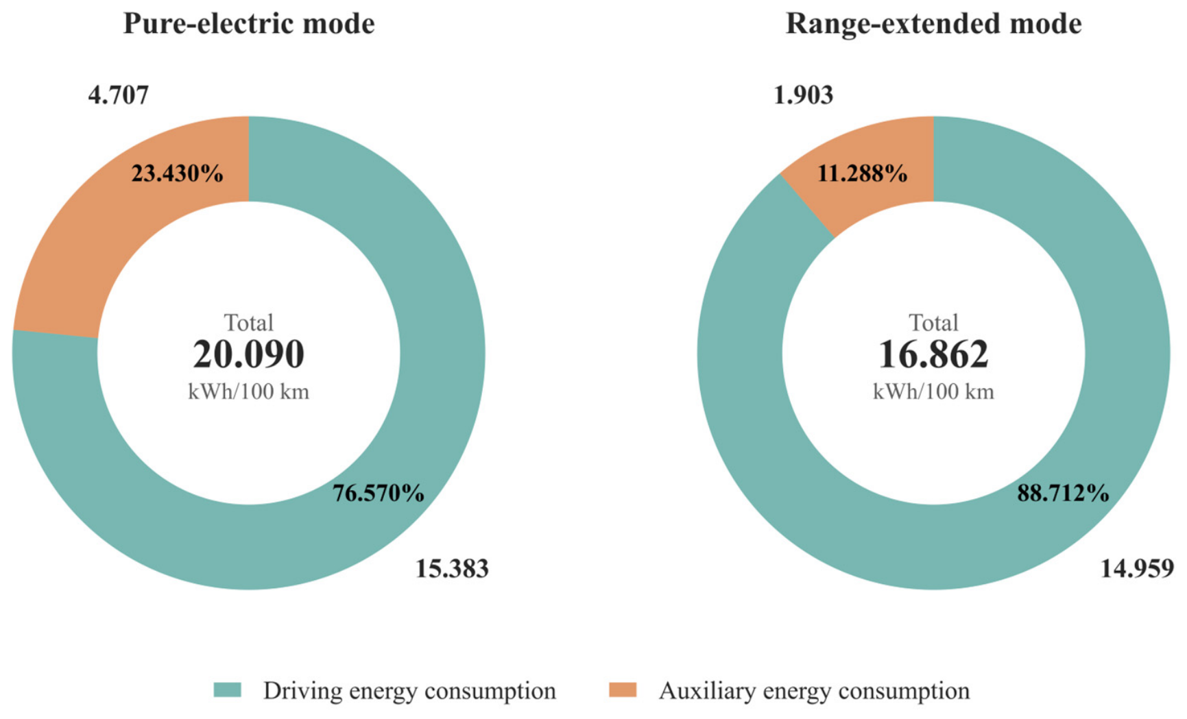
Figure 3 compares the energy composition of the test vehicle in pure-electric and range-extended modes under low-temperature conditions. Driving energy consumption was 15.383 kWh/100 km in pure-electric mode and 14.959 kWh/100 km in range-extended mode, giving a difference of only 0.424 kWh/100 km. The driving energy consumption levels were therefore similar. In contrast, auxiliary energy consumption differed substantially. It decreased from 4.707 kWh/100 km in pure-electric mode to 1.903 kWh/100 km in range-extended mode, corresponding to a reduction of 59.6%. This reduction was mainly associated with the use of engine waste heat. During range-extender operation, waste heat can directly support cabin heating and battery thermal management, thereby reducing the electrical demand of the PTC heater, compressor, and other electrically driven thermal management components. In pure-electric mode, these functions depend entirely on electrical energy. Auxiliary loads therefore accounted for a considerable proportion of total energy consumption in both modes, particularly under the increased thermal management demand at low temperatures. Overall, total energy consumption in range-extended mode was 3.228 kWh/100 km lower than that in pure-electric mode, indicating that auxiliary energy consumption was an important source of the difference between the two power modes.

3.2. Effect of Trip Scale

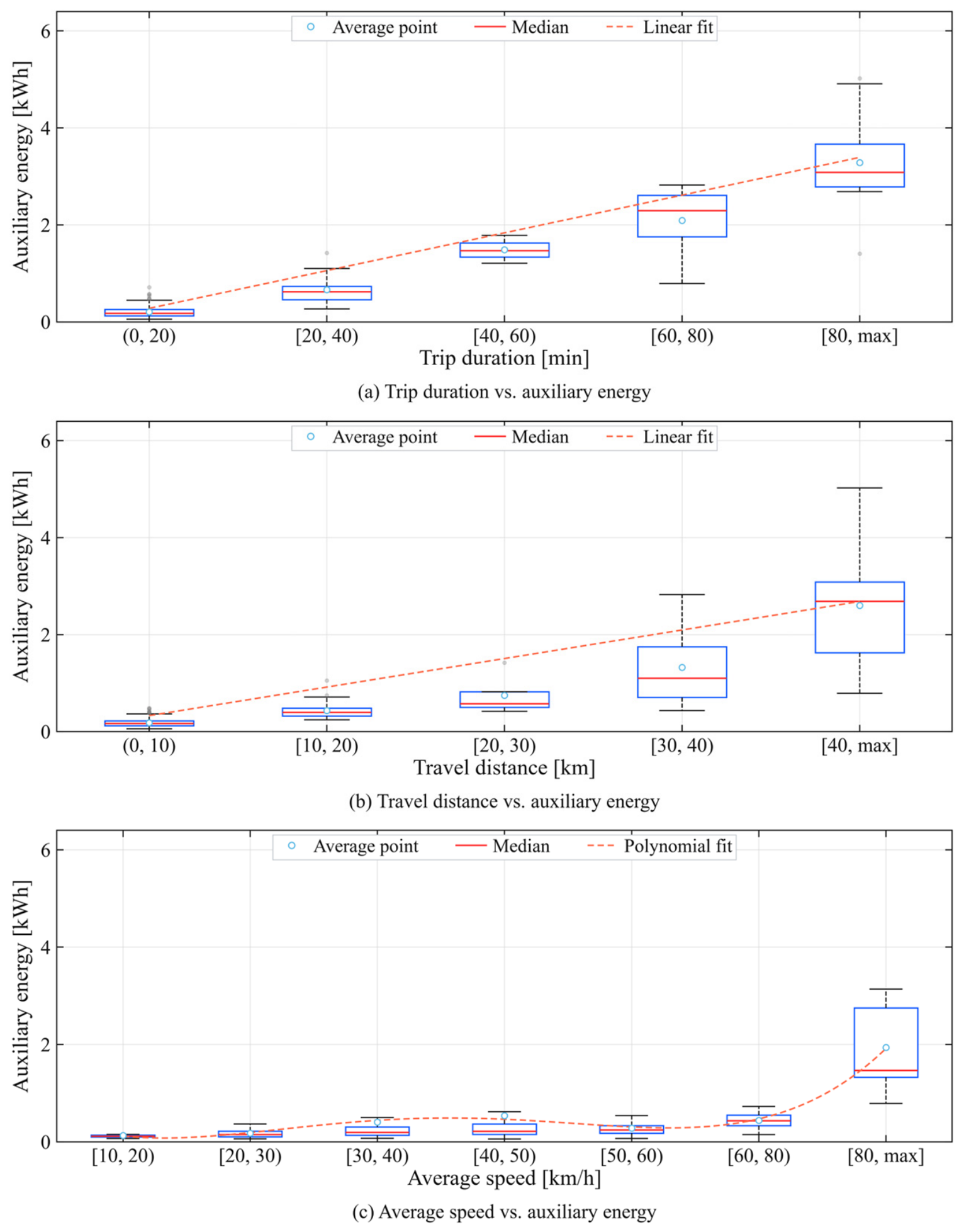
Trip scale describes the characteristics of a travel task. To identify its relationship with cumulative auxiliary energy consumption, Figure 4 presents the distribution of individual trip cumulative auxiliary energy consumption across different trip-scale intervals. Box plots show the dispersion of the samples, and interval means are used to represent the overall trends. Linear fitting was applied to trip duration and travel distance, while polynomial fitting was used for mean speed. Cumulative auxiliary energy consumption increased with both trip duration and travel distance. The PTC heater, compressor, and other auxiliary components operated continuously to maintain cabin comfort and battery temperature, so their energy use accumulated with operating time. Longer trips also generally involved longer operating periods. The relationship with mean speed was nonmonotonic. Mean auxiliary energy consumption increased from 0.130 kWh in the low-speed interval to 0.539 kWh at 40–50 km/h, decreased to 0.282 kWh at 50–60 km/h, and then increased to 1.937 kWh at mean speeds of at least 80 km/h. This nonlinear pattern reflects the combined effects of trip duration, travel distance, road type, and thermal management operating time across different speed intervals.

3.3. Effect of Thermal Management Load

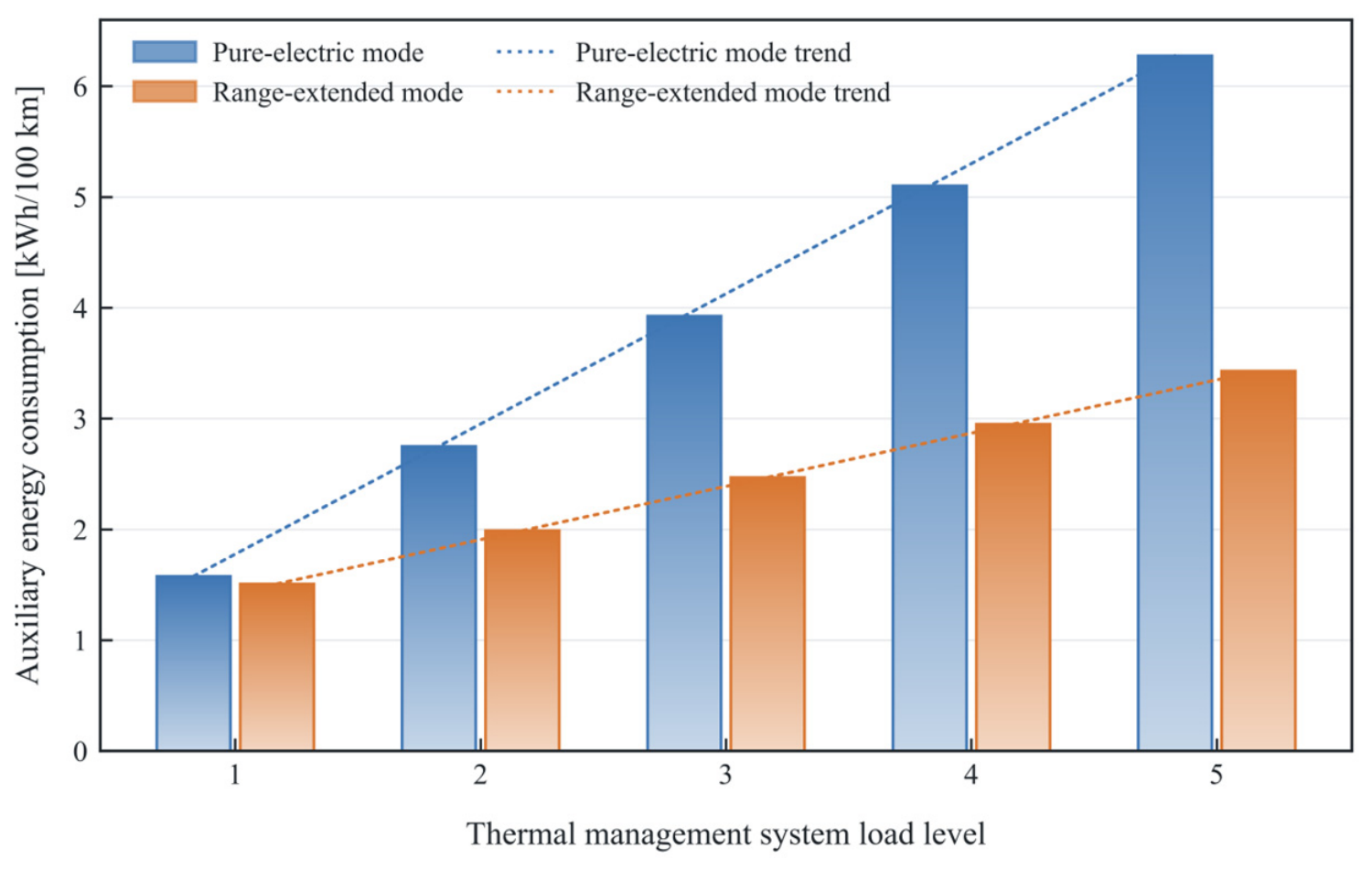
Thermal management components are major drivers of auxiliary energy consumption at low temperatures. The PTC heater and compressor were selected to represent thermal management load. Because the compressor remained active in all samples and did not provide a clear on-off gradient, its load was combined with the variable PTC load. The electrical energy of the two components was converted to mean power over each sample. Five load levels were defined, with level 1 centered at approximately 0.4 kW and each higher level increasing by about 0.5 kW. Total auxiliary energy consumption was then normalized by the actual travel distance. As shown in Figure 5, when the load increased from level 1 to level 5, auxiliary energy consumption in pure-electric mode increased from 1.576 to 6.275 kWh/100 km, while that in range-extended mode increased from 1.508 to 3.430 kWh/100 km. Although consumption increased in both modes, the increase was smaller in range-extended mode, and the difference between the modes widened from 0.068 to 2.845 kWh/100 km. In pure-electric mode, the battery powered PTC heater supplied most of the cabin- and battery heating demand, so a higher load level directly increased electrical heating consumption. In range-extended mode, waste heat carried by the coolant shared the cabin heating and battery warming demand. The PTC heater mainly maintained temperature and provided supplementary heat. These results show that the PTC heater and compressor are key drivers of low-temperature auxiliary energy consumption, while engine waste heat utilization is the main mechanism limiting the increase in electrical heating demand during range-extender operation.

3.4. Effect of Range-Extender Operating Share

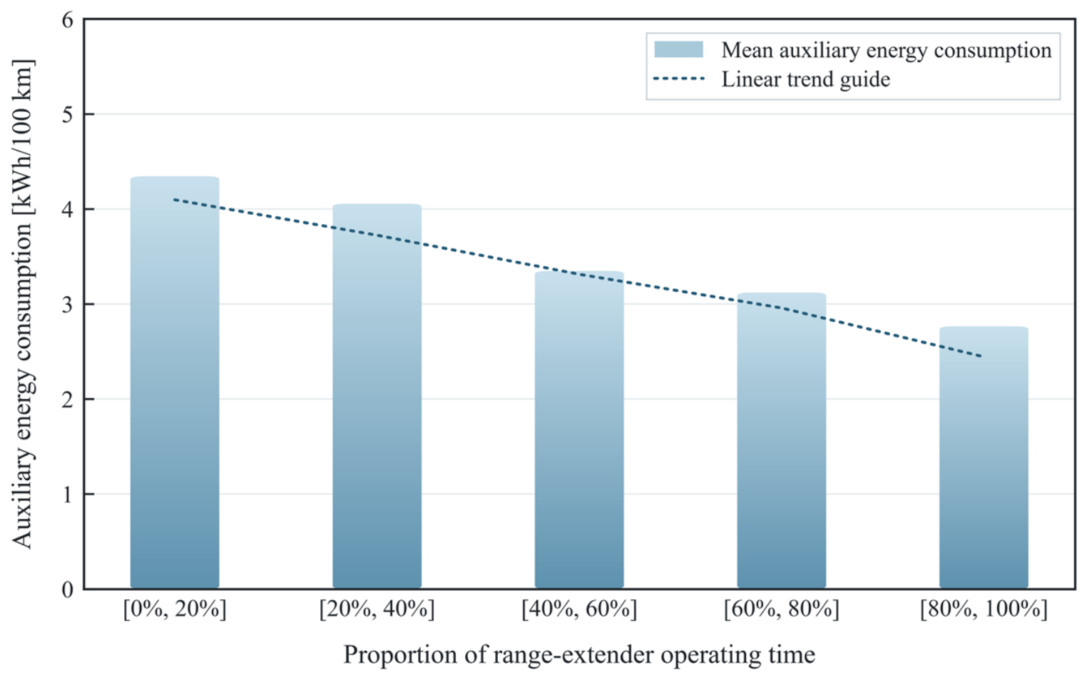
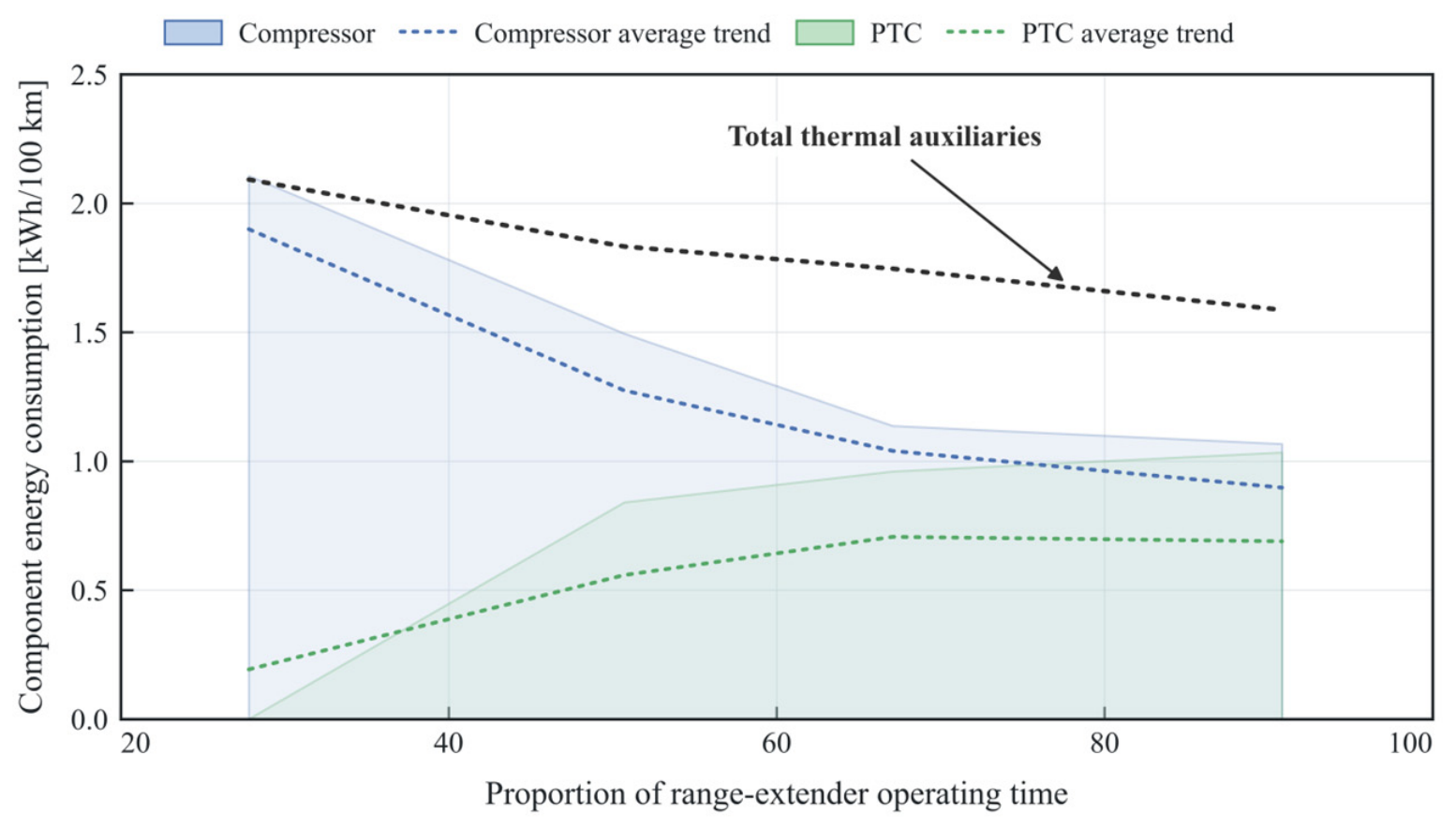
To quantify the effect of range-extender operation on auxiliary energy consumption, the range-extender operating share was divided into five intervals. As shown in Figure 6, auxiliary energy consumption decreased from 4.345 to 2.765 kWh/100 km as the operating share increased, representing a reduction of 36.4%. The electrical consumption of the PTC heater and compressor was further separated to identify the associated thermal management path (Figure 7). Compressor energy consumption decreased by 52.8%, whereas PTC energy initially increased and then gradually stabilized. Their combined effect reduced total thermal management electricity from 2.092 to 1.587 kWh/100 km, a decrease of 24.1%. Immediately after the range-extender was activated, the engine coolant had not yet reached a temperature sufficient for effective heating. Cabin and battery heating therefore remained dependent mainly on the compressor and PTC heater. As operation continued, engine waste heat was transferred to the coolant and entered the cabin and battery heat exchange circuits. This process reduced compressor load and supplied part of the sustained heating demand otherwise met by the PTC heater.

4. Development and Application of Auxiliary Energy Consumption Prediction Models

To predict REEV auxiliary energy consumption at low temperatures, this section develops models at two time scales. The trip-scale model uses navigation information and the vehicle state at departure to estimate cumulative auxiliary energy consumption for the entire trip. The second-scale model uses recent vehicle operation, traction battery state, and thermal management state to update the remaining auxiliary energy consumption during driving. Coordinating the models provides accurate, continuous prediction from departure planning through the driving stage.

4.1. Trip-Scale Auxiliary Energy Consumption Prediction Model

The trip-scale model uses the navigation task and the vehicle state at departure to provide a coarse estimate of cumulative auxiliary energy consumption for the complete trip. Variables describing the initial vehicle state were first selected. LSBoost, RF, and MLP models were then constructed and compared. Finally, SHapley Additive exPlanations (SHAP) analysis was applied to the best-performing model to quantify each input variable’s contribution to predicted trip-scale auxiliary energy consumption.

4.1.1. Candidate Variable Selection

The trip-scale model predicts cumulative auxiliary energy consumption for the entire trip from planned trip information and the vehicle state available before departure. Six inputs were selected: the trip duration t , the travel distance d , the initial state of charge S O C s t a r t , the initial compressor speed n E D C , s t a r t , the initial PTC power P P T C , s t a r t , and the initial battery temperature T b a t t , s t a r t . t and d describe the operating time of the auxiliary systems and the spatial scale of the trip; n E D C , s t a r t and P P T C , s t a r t represent the initial thermal management load. S O C s t a r t represents the energy reserve and energy management state at departure, thereby describing the trip energy supply strategy and the initial energy boundary for range-extender operation. T b a t t , s t a r t characterizes the initial battery thermal management state and its corresponding thermal boundary. In Equation (8), Z 0 is the input vector at departure, superscript T denotes vector transpose, g is the trip-scale regression model, and E a u x , t r i p is the corresponding entire trip auxiliary energy consumption. Trip duration and distance represent temporal and spatial task scale, while the four variables measured at departure describe the initial battery and thermal-management boundary.
Z 0 = t d S O C s t a r t n E D C , s t a r t P P T C , s t a r t T b a t t , s t a r t T E a u x , t r i p = g ( Z 0 )
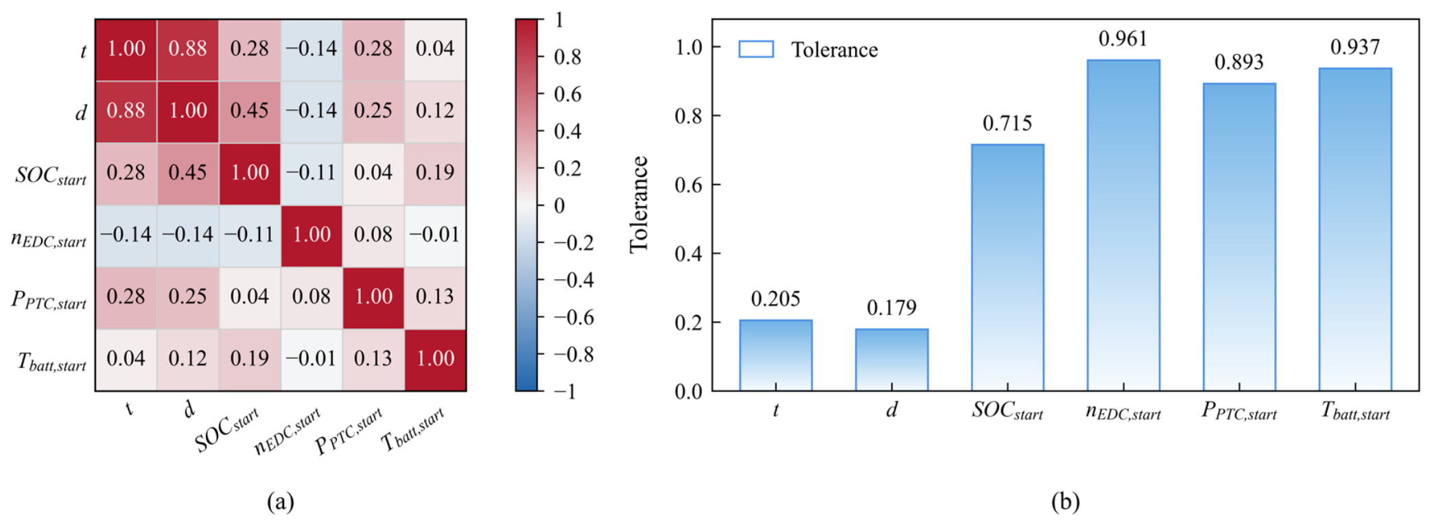
Pearson correlation analysis and tolerance-based multicollinearity testing were jointly used to identify redundant information among the candidate variables (Figure 8). The highest correlation coefficient was 0.88 between t and d , whereas the absolute coefficients of all other pairs were below 0.5. Tolerance values ranged from 0.179 to 0.961 and remained above the severe multicollinearity threshold of 0.10. Although t and d were strongly correlated, they describe different temporal accumulation and spatial characteristics of the trip and did not constitute severe multicollinearity. All six variables were therefore retained.

4.1.2. Model Development and Validation

Trip-scale samples were constructed by first identifying basic driving segments from the speed signal. Adjacent segments separated by stationary periods of no more than 120 s were merged. Samples were retained when travel distance exceeded 3 km, trip duration exceeded 300 s, and calculated auxiliary energy consumption was nonnegative, producing 165 valid samples. Thirty repeated grouped partitions were then generated using the original dataset identifier as the grouping unit, with approximately 70% of the data used for training and 30% for testing; trips from the same dataset were never assigned to both subsets. Fourfold grouped cross-validation was used for model selection. Bayesian optimization was adopted for RF and LSBoost, whereas the compact discrete MLP search space was evaluated by grid search. Hyperparameter selection was confined to grouped training data, and the resulting configurations were retained throughout the repeated grouped holdout evaluation to maintain a consistent model specification across partitions.
The input was Z 0 as defined in Equation (8), and the output was E a u x , t r i p . Bayesian optimization used a Gaussian-process surrogate and the expected-improvement-plus acquisition function, with 25 objective evaluations and fourfold grouped cross-validated RMSE as the objective. For LSBoost, the search ranges were 100–600 learning cycles, 0.01–0.20 learning rate (log scale), 5–100 maximum splits, and 2–30 minimum leaf size. For RF, 200–800 trees, 1–30 minimum leaf size, 20–500 maximum splits, and 2–6 sampled predictors were considered. MLP grid search evaluated LayerSizes ∈ {4, 5, 6, 8, [4, 2], [5, 2], [6, 3], [8, 4]}, λ ∈ {0.5, 0.7, 1, 3, 10}, and IterationLimit ∈ {60, 100, 140}, with ReLU activation and response standardization fixed. The predictive results and selected configurations are listed in Table 2 and Table 3. RF achieved the highest mean test-set R2 and low mean RMSE and MAE values, indicating that its ensemble structure captured nonlinear interactions between trip scale and the initial vehicle state.

4.1.3. SHAP Value Analysis of the Trip-Scale Model

Conventional validation metrics quantify predictive accuracy but do not show how the nonlinear RF model uses each input to produce its predictions. The RF model was analyzed using SHAP values to explain how trip scale and the initial vehicle state influenced each prediction. Based on the Shapley value from cooperative game theory, SHAP quantifies the contribution of each feature to an individual prediction. For the trip-scale model, SHAP analysis reveals the direction and relative strength of the effects of trip task and departure state variables on predicted cumulative auxiliary energy consumption.
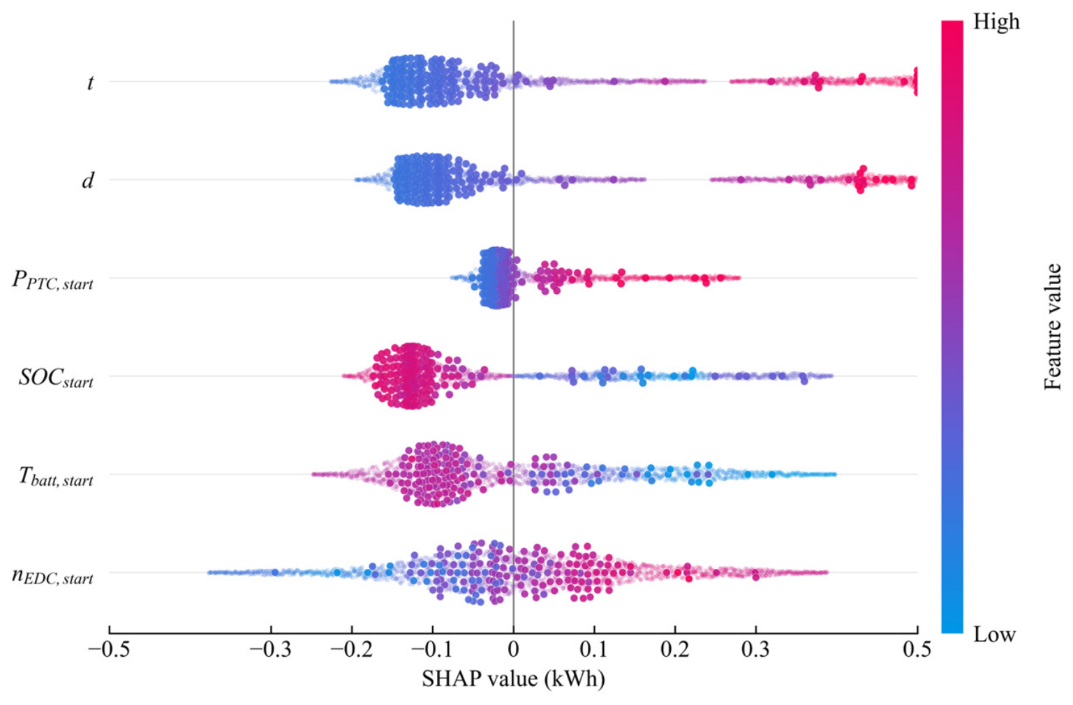
Figure 9 presents the distribution of SHAP values for the RF model. Trip duration t and travel distance d had substantially wider SHAP ranges than the other variables and were the dominant inputs. High values of both variables were mainly located in the positive SHAP region. Longer trips extend the operating time of thermal-management, air conditioning, and other auxiliary components, thereby increasing predicted auxiliary energy consumption. High initial PTC power P P T C , s t a r t also tended to produce positive SHAP values. Initial battery temperature T b a t t , s t a r t and initial state of charge S O C s t a r t showed clearer inverse patterns, with high values appearing more frequently in the negative SHAP region. Initial compressor speed n E D C , s t a r t had the smallest contribution because it represented only the instantaneous departure state and not subsequent changes.
Based on the feature-level SHAP results described above, the six input variables were further classified into three groups: trip-scale information, initial battery state variables, and initial auxiliary load variables. For each input feature j its importance S j was calculated as the mean absolute SHAP value across the Q samples included in the SHAP analysis:
S j = 1 Q q = 1 Q ϕ q j
where ϕ q j is the SHAP value of feature j for sample q . The percentage contribution C G of feature group G was then calculated as
C G = j G S j j = 1 J S j × 100 %
where G denotes a given feature group and J is the total number of input features ( J = 6). The numerator is the sum of the mean absolute SHAP values of the features within a given group, whereas the denominator is the corresponding sum for all six input features. This normalization makes the contributions of the three feature groups directly comparable, with their percentages summing to 100%.
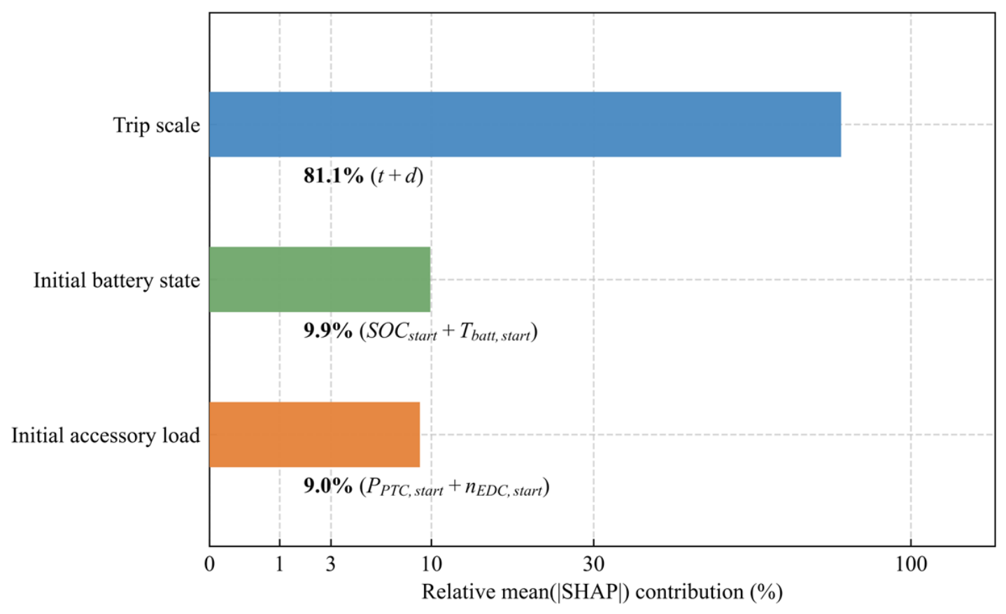
Figure 10 groups the input variables according to their mean absolute SHAP values. Trip-scale information contributed 81.1% of the total importance and was the main information source used by RF. Initial battery state variables and initial auxiliary load variables contributed 9.9% and 9.0%, respectively. These results confirm that trip duration and travel distance primarily determine the cumulative operating demand of auxiliary systems. Initial PTC power, compressor speed, SOC, and battery temperature provide complementary information on thermal management demand and battery state at departure. Overall, the contribution results show a clear difference among the three types of input variables. Trip-scale information provides most of the information required by RF, while initial battery state variables and initial auxiliary load variables provide additional information. Together, these variables describe both the cumulative operating demand of auxiliary systems during the trip and the thermal management demand and battery state at departure, thereby supporting RF in predicting auxiliary energy consumption at the trip scale.

4.2. Second-Scale Auxiliary Energy Consumption Prediction Model

The trip-scale model can estimate entire trip auxiliary energy consumption before departure, but it cannot represent continuous changes in vehicle state and thermal management load during driving. A second-scale model was therefore developed to predict remaining auxiliary energy consumption. Development included aggregated sample construction, candidate variable selection, algorithm comparison, and sample duration comparison. For each sample, two targets were calculated: mean auxiliary power within the current interval and mean auxiliary power over the remaining trip. The first target compared the ability of different algorithms and durations to represent dynamic auxiliary load. The second was used to calculate remaining auxiliary energy consumption.

4.2.1. Sample Construction and Variable Selection

Let τ k denote the end time of update k and L the aggregation duration. Inputs were aggregated over τ k L , τ k . Durations of 5, 10, 15, 20, 30, and 60 s were evaluated. Samples outside basic physical ranges and other abnormal samples were removed. The six durations yielded 48,880, 24,368, 16,072, 11,961, 7817, and 3691 valid second-scale samples, respectively.
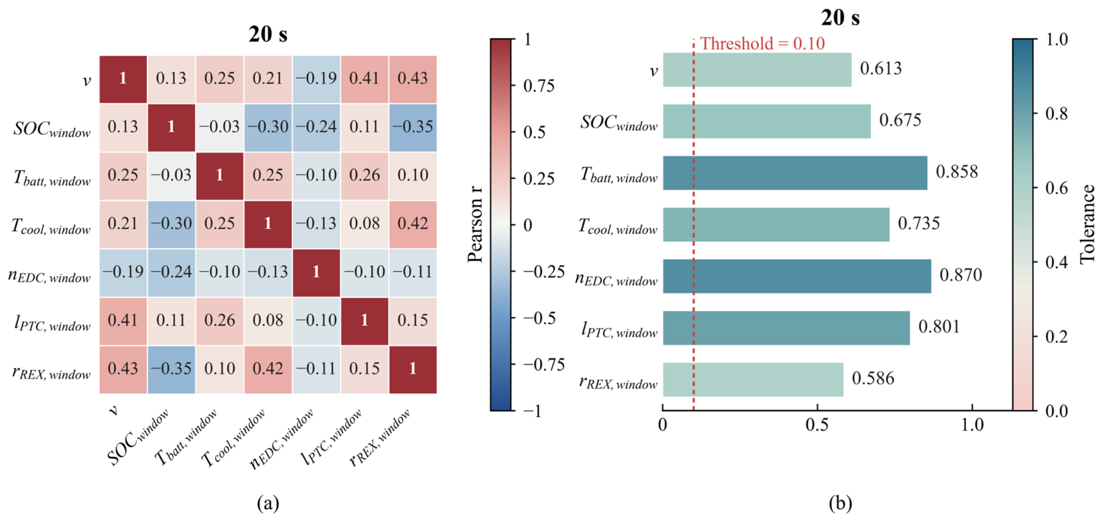
Seven candidate inputs were selected: the mean vehicle speed v ¯ , the mean state of charge S O C w i n d o w , the mean battery temperature T b a t t , w i n d o w , the mean engine coolant temperature T c o o l , w i n d o w , the mean compressor speed n E D C , w i n d o w , the PTC operating level l P T C , w i n d o w , and the range-extender operating share r R E X , w i n d o w . For a fixed L , travel distance is directly related to mean speed; the remaining variables describe current battery, thermal-management, and range-extender states. The maximum correlation coefficient and minimum tolerance remained within the adopted limits. Equation (11) defines the input vector X k L , and Equation (12) defines the each sample mean power prediction P ^ a u x , w i n , k L ; the f w i n L denotes the second-scale model trained for duration L . These symbols are used consistently in the integrated framework.
X k L = v ¯ S O C w i n d o w T b a t t , w i n d o w T c o o l , w i n d o w n E D C , w i n d o w l P T C , w i n d o w r R E X , w i n d o w T
P ^ a u x , w i n , k L = f w i n L ( X k L )
Because the same candidate variables were used for all durations, Figure 11 presents the correlation and tolerance diagnostics for the 20 s sample duration as an example. For the representative 20 s duration, the maximum absolute Pearson correlation coefficient was 0.43, and the minimum tolerance was 0.586; both remained within the adopted limits. The seven variables therefore provided sufficiently independent state information and were all retained for predicting remaining auxiliary energy consumption.

4.2.2. Model Development and Validation

To evaluate model and aggregation duration effects, LSBoost, RF, and MLP models were constructed for all six durations. For each duration, a fixed random seed generated four outer folds at the window sample level, ensuring consistent partitions across models and durations. The resulting metrics characterize predictive performance across the vehicle operating and thermal management conditions represented in the dataset, rather than performance under a separate trip level evaluation. In each outer iteration, three folds were used for training and one for validation. Hyperparameters were selected exclusively from the outer training data through inner fourfold cross validation, using Bayesian optimization for RF and LSBoost and grid search for MLP. Each optimized model was refitted on the outer training data and evaluated on the validation fold. R2, RMSE, and MAE were averaged across the four folds. This nested procedure prevented validation data from contributing to hyperparameter selection and supported comparison of the algorithms and aggregation durations.
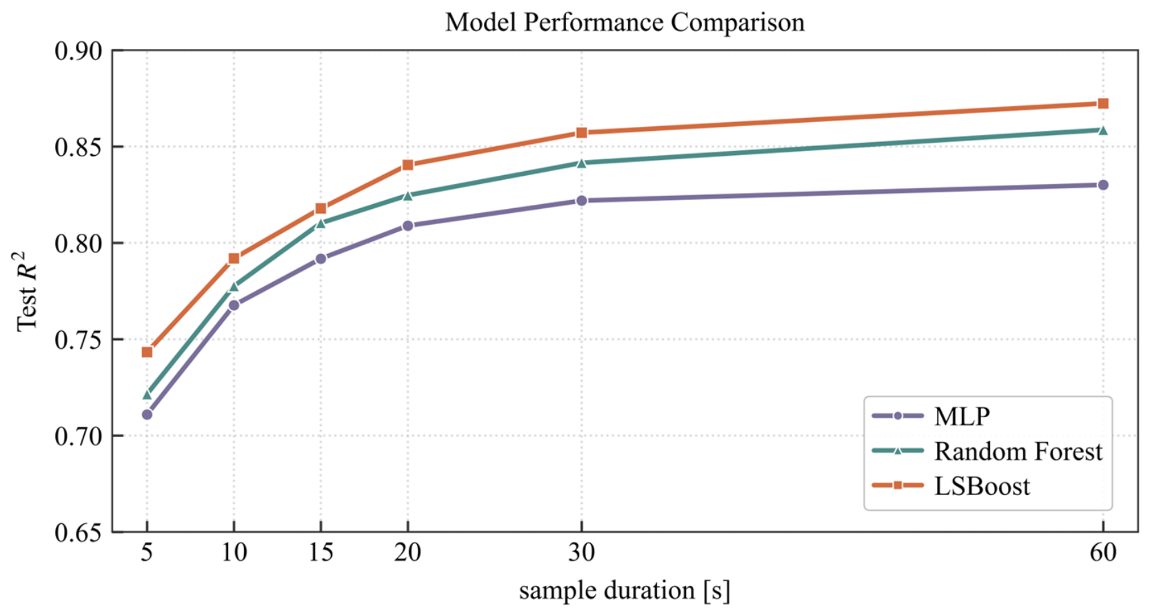
Figure 12 shows the test-set R2 values of the three models for six sample durations. Prediction accuracy generally increased as duration increased from 5 to 60 s. A moderately longer sample duration reduces fluctuations and provides a more stable representation of vehicle operation, battery state, and thermal management load. At the same time, an excessively long sample duration lowers the update frequency and further smooths short-term state variations, allowing prediction errors to persist until the next update and thereby weakening support for real-time vehicle decision-making. LSBoost maintained high accuracy at all durations, indicating that its iterative residual fitting mechanism captured nonlinear relationships, local variations, and threshold changes between the current state variables and auxiliary power. However, the improvement diminished as duration approached 60 s, suggesting that temporal aggregation provided limited gains and that model performance was approaching a stable range.
Table 4 provides detailed results for the three models at each sample duration. As duration increased, test-set R2 generally increased, while RMSE and MAE decreased. This trend confirms that a longer aggregation range can reduce instantaneous fluctuations and improve the stability of information representing current auxiliary load. For LSBoost, test-set R2 increased from 0.743 at 5 s to 0.857 at 30 s, while RMSE decreased from 0.397 to 0.245 kW and MAE decreased from 0.289 to 0.183 kW. At 60 s, R2 reached 0.872, with an RMSE of 0.210 kW and an MAE of 0.159 kW. The improvement from 30 to 60 s was smaller than that observed at shorter durations, indicating that the benefit of further temporal aggregation gradually diminished. RF and MLP exhibited similar trends, with only limited accuracy gains at longer durations, suggesting that model performance was approaching a stable level.

4.3. Integrated Application of the Two Models

The trip-scale and second-scale models were combined to provide continuous auxiliary energy consumption prediction before departure and during vehicle operation. The algorithm and sample duration were selected according to their performance in predicting mean auxiliary power within each sample. The corresponding model was then used to predict mean auxiliary power over the remaining trip and calculate remaining auxiliary energy consumption. The trip-scale model provides the initial estimate for the entire trip. During driving, the second-scale model predicts remaining auxiliary energy consumption, which is combined with the measured cumulative auxiliary energy consumption to update the entire trip estimate.

4.3.1. Two-Stage Integrated Prediction Framework

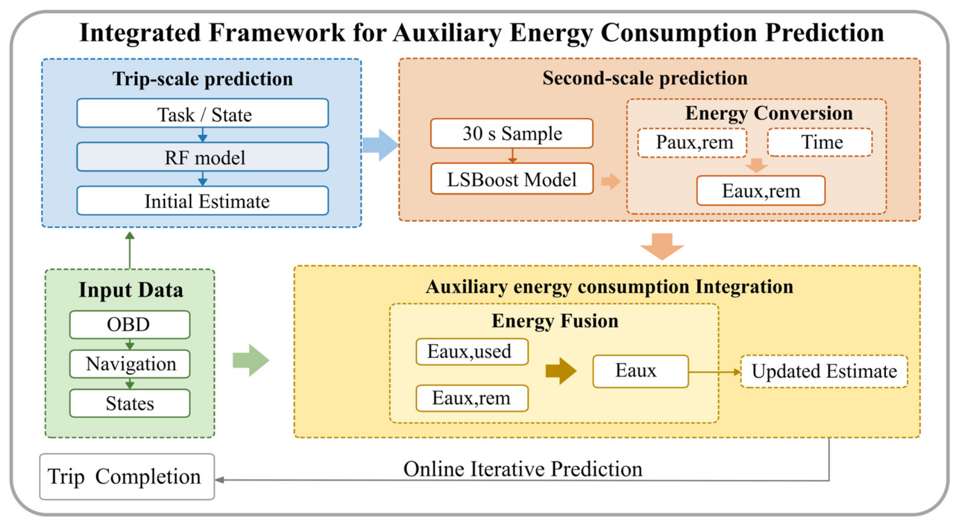
The two models perform different tasks according to the information available before departure and during driving. Before departure, the trip-scale RF model predicts auxiliary energy consumption for the entire trip using planned trip information and initial vehicle states. The planned trip duration and travel distance are obtained from the onboard navigation system based on GPS (Global Positioning System) positioning and route planning, while the initial SOC, the battery temperature, the PTC power, and the compressor speed are acquired through the CAN bus and telematics system. After departure, the second-scale model uses updated vehicle states to predict mean auxiliary power over the remaining trip. This power is converted to remaining auxiliary energy consumption using updated remaining travel time and combined with measured cumulative consumption to iteratively update the entire trip estimate.
Let Z 0 denote the planned trip and departure condition vector. The trip-scale model provides the initial entire trip prediction:
E ^ a u x , 0 = g ( Z 0 )
where E ^ a u x , 0 is the entire trip auxiliary-energy prediction at departure and g is the trip-scale RF model defined in Equation (8).
After departure, let Δ t u be the prediction update interval and τ k = k Δ t u the time of update k . This update interval is distinct from the acquisition sampling interval Δ t s in Equation (1). At τ k , vehicle states and auxiliary energy consumption from trip origin to the current position have been observed. Cumulative consumption is
E a u x , u s e d , k = 1 3600 0 τ k P a u x ( s ) d s
where E a u x , u s e d , k is cumulative auxiliary energy consumed by update k ; P a u x ( s ) is instantaneous measured auxiliary power (kW).
At update k , vehicle states over τ k L , τ k are aggregated into X k L . The remaining-demand model then predicts mean auxiliary power from the current position to trip end:
P ^ a u x , r e m , k = f r e m L ( X k L )
where P ^ a u x , r e m , k is predicted mean auxiliary power over the remaining trip and f r e m L is the second-scale model using aggregation duration L .
Using the remaining travel time available at the current update, predicted remaining auxiliary energy consumption is
E ^ a u x , r e m , k = P ^ a u x , r e m , k T r e m , k 3600
where E ^ a u x , r e m , k is predicted remaining auxiliary energy at update k and T r e m , k is remaining travel time (s) supplied by the navigation system. The updated prediction of entire trip auxiliary energy consumption after update k is
E ^ a u x , k = E a u x , u s e d , k + E ^ a u x , r e m , k
Here, E ^ a u x , k is the dynamically updated entire trip estimate. Equation (17) combines measured consumption from the completed segment, E a u x , u s e d , k , with predicted consumption for the remaining segment, E ^ a u x , r e m , k , allowing the estimate to refresh as operating state observations and navigation time are updated.

4.3.2. Application of the Integrated Model

LSBoost was selected for the integrated prediction of remaining auxiliary energy consumption according to the results in Section 4.2.2. The prediction update interval determines how frequently the model receives the latest vehicle states and refreshes its prediction. A shorter interval reflects state changes more promptly but increases data aggregation and onboard computation. A longer interval reduces computational frequency but allows more state changes to accumulate between predictions, reducing input timeliness. LSBoost achieved a test-set R2 of 0.857 with a 30 s sample duration. Extending the sample duration to 60 s increased R2 by only 0.015. The prediction update interval was therefore set to 30 s to align state aggregation with prediction updates while balancing accuracy, timeliness, and onboard computational load. Figure 13 shows the resulting process.
An additional holdout evaluation used 1281 samples with a duration of 30 s. Normalized trip progress was divided into five intervals, and approximately 20% of the samples in each interval were selected for the holdout set. To assess prediction errors over a wider sample range, the absolute error between the dynamically updated entire trip auxiliary energy prediction and the measured value was calculated for each sample, with the statistical results summarized in Table 5. The MAE and RMSE were 0.014 and 0.032 kWh, respectively. The standard deviation of absolute errors was 0.029 kWh, while the 90th and 95th percentile values were 0.030 and 0.048 kWh. These results indicate generally small prediction deviations across the holdout samples, despite some variation among individual prediction points.
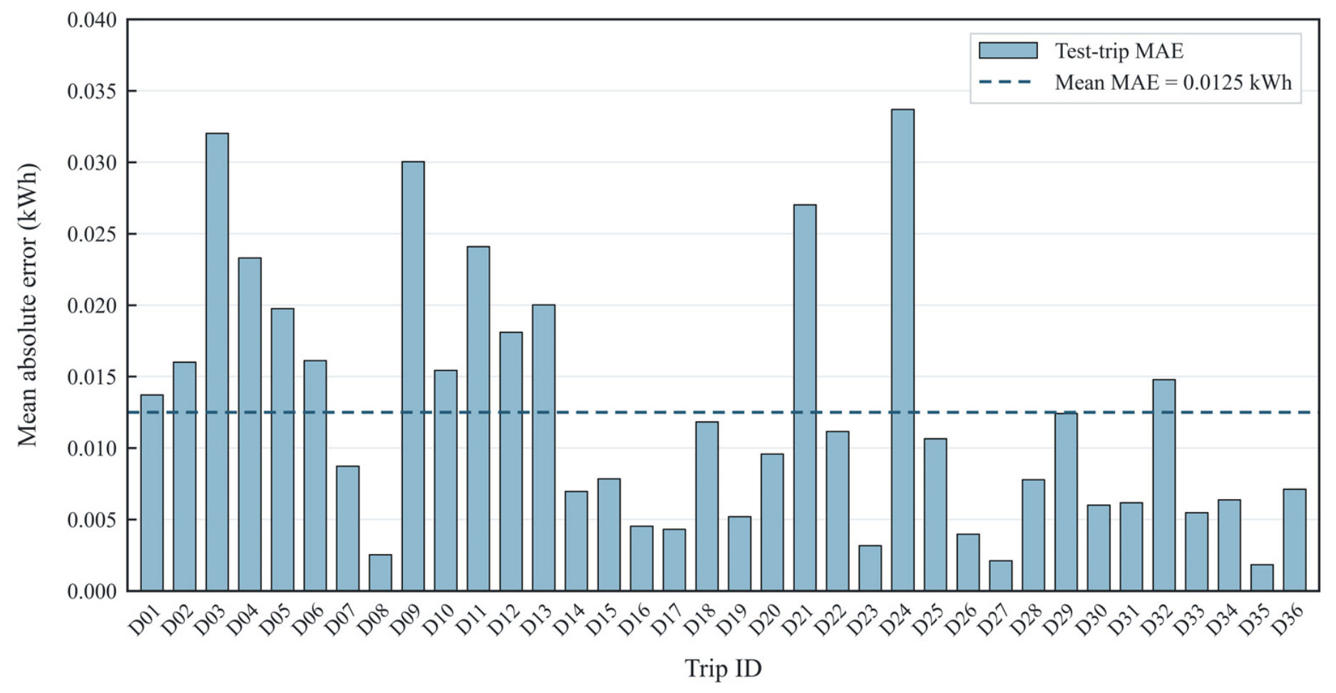
To further assess prediction performance across trips, the 1281 final holdout samples were grouped by TripID, yielding 36 test trips. For each trip, the MAE was calculated as the mean absolute difference between the dynamically updated entire trip auxiliary energy prediction and the measured value. As shown in Figure 14, the MAEs for individual trips ranged from 0.002 to 0.034 kWh, with an average of 0.013 kWh across the 36 test trips. This analysis enables a direct comparison of prediction errors across all trips represented in the final holdout set. And the trip D14 was further selected as a representative example to illustrate the iterative prediction process. Its measured auxiliary energy consumption was 2.692 kWh, its duration was 6262.29 s, and its total distance was 172.27 km. At departure, the trip-scale RF model provided the initial estimate for the entire trip. After the vehicle began moving, the second-scale LSBoost model predicted mean auxiliary power over the remaining trip at 30 s sample duration.
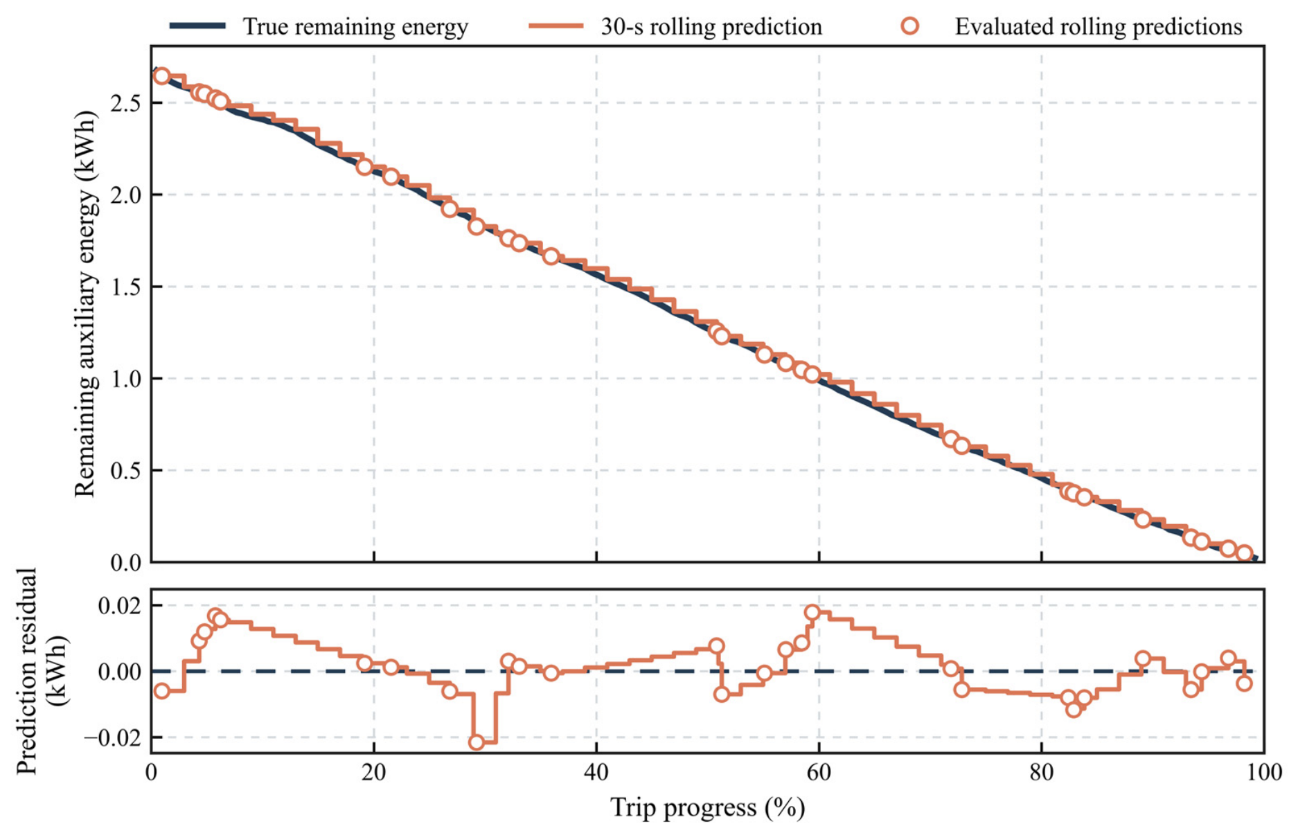
Figure 15 presents the iterative trajectory and residuals of predicted remaining auxiliary energy consumption for the representative trip. Measured remaining auxiliary energy consumption decreased continuously as the trip progressed, and the predicted trajectory generally followed this trend. Stepwise changes resulted from the 30 s prediction update interval. Local sawtooth fluctuations reflected changes in vehicle speed, thermal management load, and range-extender operating state that affected predicted mean auxiliary power over the remaining trip. They did not indicate instability. The mean absolute residual was 0.008 kWh during the first 40% of the trip and decreased to 0.005 kWh after 60% progress. All residuals were within 0.022 kWh. The 30 s LSBoost model therefore used the latest dynamic states to maintain low error throughout the trip.
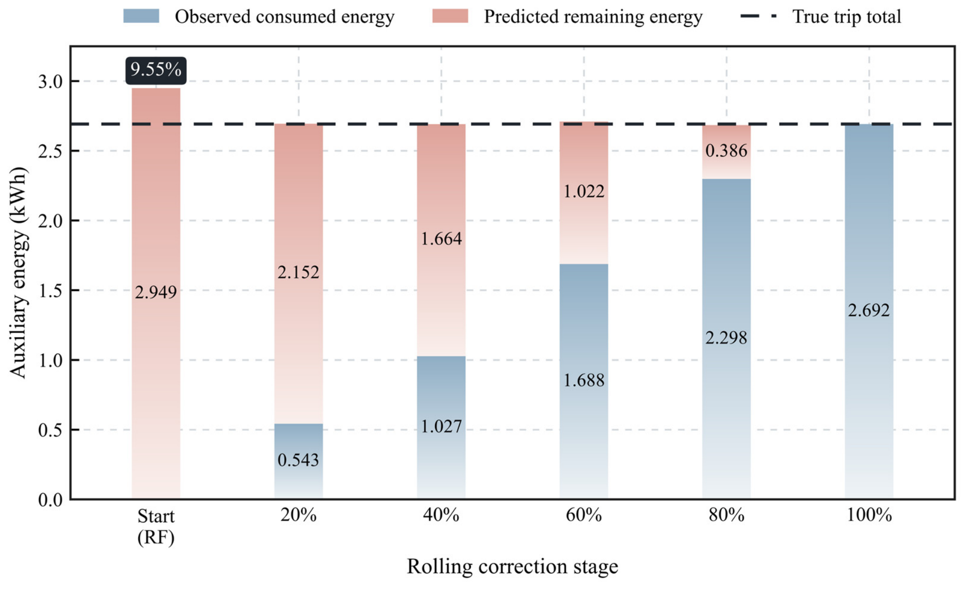
Figure 16 separates the integrated prediction into its energy components. At departure, RF predicted entire trip auxiliary energy consumption of 2.949 kWh, an error of 9.55% relative to the measured 2.692 kWh. During second-scale updating, each entire trip estimate combined measured cumulative auxiliary energy consumption with predicted remaining auxiliary energy consumption. At 20%, 40%, 60%, and 80% progress, the updated estimates were 2.695, 2.691, 2.710, and 2.684 kWh, respectively, and remained close to the measured total. As the trip progressed, measured cumulative auxiliary energy consumption contributed more and predicted remaining auxiliary energy consumption contributed less. Changes in thermal management load and range-extender operating state caused small local fluctuations, but the overall prediction error remained low.

4.3.3. Comparison with Recent Energy Prediction Studies

Table 6 positions this study against recent energy prediction research using three dimensions: vehicle context, prediction target, and modeling framework. Existing electric vehicle energy prediction studies have mainly focused on total or traction energy consumption, whereas dedicated prediction of auxiliary energy remains relatively limited, and most related studies have focused on BEVs. Low-temperature REEV operation introduces an additional interaction among range-extender participation, recoverable engine heat, and electrically supplied thermal management, because engine waste heat can partly meet cabin and battery heating demands and thereby alter auxiliary energy consumption. Meanwhile, existing auxiliary energy studies generally treat predictions at different temporal scales as separate tasks, which leaves scope for a unified framework that links initial whole-trip estimation with subsequent updates during driving.
Schäfers et al. [20] investigated BEV auxiliary systems and predicted auxiliary power and trip auxiliary energy, demonstrating the feasibility of separately modeling auxiliary demand from propulsion energy. However, auxiliary power and trip energy prediction were not integrated into a framework for continuously updating the whole-trip auxiliary energy estimate during driving. Kim et al. [23] further developed trip-based and seconds-based auxiliary energy prediction models for commercial BEVs using real-world vehicle data. However, the two temporal scales were modeled independently rather than being coupled to update the remaining auxiliary energy during a trip. These studies therefore differ mainly in their prediction scope and in the way predictions at different temporal scales are organized within the modeling framework.
Overall, comparison with existing studies indicates that the present work extends auxiliary energy prediction to low-temperature REEV operation, where range-extender participation and engine waste-heat utilization directly affect electrical thermal-management demand. The principal advance lies in coupling initial trip-scale estimation with repeated second-scale updating rather than treating predictions at different temporal scales independently. The trip-scale RF model provides the initial whole-trip auxiliary energy estimate, while the 30 s LSBoost model uses newly observed vehicle and thermal states to predict the remaining auxiliary energy during driving. Measured cumulative consumption is then combined with the predicted remaining energy to iteratively update the whole-trip estimate. This integrated framework therefore incorporates the specific thermal-energy characteristics of REEVs and links initial whole-trip estimation with in-trip remaining-energy prediction within a unified auxiliary energy prediction framework.

5. Conclusions

This study examined REEV auxiliary energy consumption in actual user travel scenarios at low temperatures and developed corresponding prediction models. It provides detailed characterization and accurate multiscale prediction of REEV auxiliary energy consumption. The results can support further development of whole-vehicle energy prediction systems for new energy vehicles and have important theoretical and engineering value for improving vehicle energy management. The main conclusions are as follows:
(1)
Vehicle auxiliary energy consumption data were collected in Wuhan. The tests yielded more than 3600 km of actual road driving data for the analysis.
(2)
Auxiliary energy consumption was analyzed in terms of power mode, trip scale, thermal management load, and range-extender operating share. Engine waste heat reduced auxiliary energy consumption by more than 59% in range-extended mode relative to pure-electric mode. Cumulative auxiliary energy consumption increased with trip duration and travel distance. As thermal management load increased, auxiliary energy consumption rose much more slowly in range-extended mode than in pure-electric mode. A higher range-extender operating share reduced auxiliary energy consumption by 36.4%, while total thermal management electricity decreased by 24.1%.
(3)
RF, LSBoost, and MLP were used to develop and compare the trip-scale and second-scale models. RF provided the best trip-scale performance, with test-set R2, RMSE, and MAE values of 0.826, 0.317 kWh, and 0.112 kWh, respectively. For the selected 30 s sample duration, LSBoost achieved the optimal balance between prediction performance and update timeliness, with corresponding values of 0.857, 0.245 kW, and 0.183 kW. These results support the use of RF for whole trip estimation and LSBoost for dynamic modeling over short sample durations.
(4)
SHAP analysis showed that trip-scale variables contributed more than 80% of RF model importance and dominated the prediction of entire trip auxiliary energy consumption from the departure state. Initial battery state and auxiliary load variables provided additional information on energy and thermal conditions at departure.
(5)
The trip-scale and second-scale models were integrated to provide an initial estimate before departure and dynamic updates during driving. The initial entire trip prediction error was 9.55%. Between 20% and 80% trip progress, the updated estimates ranged from 2.684 to 2.710 kWh, compared with a measured value of 2.692 kWh, and the maximum residual was 0.022 kWh. The integrated framework therefore substantially corrected the initial estimate as operating information became available in real time.
The proposed framework links an initial estimate of entire trip auxiliary energy consumption with iterative prediction of remaining auxiliary energy consumption during driving, thereby supporting auxiliary load assessment and energy management for REEVs under low-temperature conditions. The present validation covers a single vehicle, one geographical region, and a relatively narrow winter temperature range, while broader vehicle, regional, and thermal conditions remain to be examined. Future work will extend the dataset to include additional vehicles, regions, and temperature ranges, thereby further examining the applicability of the proposed framework under more diverse operating conditions.

Author Contributions

Conceptualization, H.Y., H.Z. and Y.L. (Yu Liu); methodology, H.Y. and Z.W.; software, H.Y. and Z.W.; validation, Z.W., J.L. and F.W.; formal analysis, H.Y., Z.W. and J.L.; investigation, H.Y., Z.W., J.L., F.W. and Y.L. (Yongkai Liang); resources, H.Z. and Y.L. (Yongkai Liang); data curation, H.Y., Z.W. and J.L.; writing—original draft preparation, H.Y.; writing—review and editing, H.Y., Z.W., J.L., H.Z. and Y.L. (Yongkai Liang); visualization, H.Y. and Z.W.; supervision, H.Z. and Y.L. (Yu Liu); project administration, H.Z.; funding acquisition, Y.L. (Yu Liu). All authors have read and agreed to the published version of the manuscript.

Funding

This research was funded by the Tianjin Key Research and Development Program, grant number 25YFYFFG01730.

Data Availability Statement

Dataset available on request from the authors.

Conflicts of Interest

The authors Hanzhengnan Yu, Hao Zhang and Yu Liu were employed by the company China Automotive Technology and Research Center Co., Ltd., Tianjin, China; the authors Hanzhengnan Yu, Jingyuan Li, Fengbin Wang and Yongkai Liang were employed by the company CATARC Automotive Test Center (Tianjin) Co., Ltd., Tianjin, China. The remaining authors declare that the research was conducted in the absence of any commercial or financial relationships that could be construed as a potential conflict of interest.

Abbreviations

The following abbreviations are used in this manuscript:
BEVbattery electric vehicle
CANcontroller area network
DCDirect Current
ECUelectronic control unit
EDCelectrically driven compressor
F.S.full scale
GBGradient Boosting
GPSGlobal Positioning System
HVACheating, ventilation, and air conditioning
LSTMLong Short-Term Memory
LSBoostLeast-Squares Boosting
MAEmean absolute error
MAPEmean absolute percentage error
MLPMultilayer Perceptron
MSEmean squared error
OBD-IIonboard diagnostics II
PTCpositive temperature coefficient
REEVrange-extended electric vehicle
ReLUrectified linear unit
REXrange-extender
RFRandom Forest
RMSEroot mean square error
SHAPSHapley Additive exPlanations
SOCstate of charge
XGBoostextreme gradient boosting

References

  1. Kumawat, P.; Weller, K.; Potturu, L.; Borken-Kleefeld, J. NOx emission deterioration in modern trucks: Evidence from remote sensing. Sci. Total Environ. 2025, 1008, 180989. [Google Scholar] [CrossRef] [Scilit]
  2. Meng, Z.; Zhou, F.; Duan, X.; Fu, J.; Liu, J.; Deng, B. Experimental study of the effects of engine oil on gaseous and particulate emissions during gasoline/ethanol combustion. Fuel 2025, 386, 134331. [Google Scholar] [CrossRef] [Scilit]
  3. Yañez, C.C.; Bares, R.; Czimczik, C.I.; Lin, J.; Zhang, J.; Bush, S.; Hopkins, F.M. Contrasting summertime trends in vehicle combustion efficiency in Los Angeles, CA, and Salt Lake City, UT. Environ. Sci. Technol. 2025, 59, 1287–1297. [Google Scholar] [CrossRef] [Scilit]
  4. International Energy Agency. World Energy Outlook 2025; IEA: Paris, France, 2025; Available online: https://www.iea.org/reports/world-energy-outlook-2025 (accessed on 24 July 2026).
  5. Chen, X.; Wang, X. Effects of carbon emission reduction policies on transportation mode selections with stochastic demand. Transp. Res. Part E Logist. Transp. Rev. 2016, 90, 196–205. [Google Scholar] [CrossRef] [Scilit]
  6. Zhang, N.; Lu, Y.; Hajabdollahi Ouderji, Z.; Yu, Z. Review of heat pump integrated energy systems for future zero-emission vehicles. Energy 2023, 273, 127101. [Google Scholar] [CrossRef] [Scilit]
  7. Yan, M.; Chen, S.; Sun, Y.; Wang, Y.; Li, M. Altruistic energy management strategy for connected new energy vehicles. Energy 2026, 356, 141269. [Google Scholar] [CrossRef] [Scilit]
  8. Ilyushin, Y.V.; Novozhilov, I.M. Software implementation of a pulse regulator of a distributed distributed control object. In Proceedings of the 2017 IEEE 2nd International Conference on Control in Technical Systems (CTS), St. Petersburg, Russia, 25–27 October 2017; pp. 315–317. [Google Scholar] [CrossRef] [Scilit]
  9. Genikomsakis, K.N.; Mitrentsis, G. A computationally efficient simulation model for estimating energy consumption of electric vehicles in the context of route planning applications. Transp. Res. Part D Transp. Environ. 2017, 50, 98–118. [Google Scholar] [CrossRef] [Scilit]
  10. Gallet, M.; Massier, T.; Hamacher, T. Estimation of the energy demand of electric buses based on real-world data for large-scale public transport networks. Appl. Energy 2018, 230, 344–356. [Google Scholar] [CrossRef] [Scilit]
  11. Beckers, C.J.J.; Besselink, I.J.M.; Frints, J.J.M.; Nijmeijer, H. Energy consumption prediction for electric city buses. In Proceedings of the 13th ITS European Congress, Eindhoven, The Netherlands, 3–6 June 2019; Available online: https://research.tue.nl/en/publications/energy-consumption-prediction-for-electric-city-buses/ (accessed on 18 August 2026).
  12. Abdelaty, H.; Mohamed, M. A framework for BEB energy prediction using a low-resolution open-source data-driven model. Transp. Res. Part D Transp. Environ. 2022, 103, 103170. [Google Scholar] [CrossRef] [Scilit]
  13. Zhang, J.; Wang, Z.; Liu, P.; Zhang, Z. Energy consumption analysis and prediction of electric vehicles based on real-world driving data. Appl. Energy 2020, 275, 115408. [Google Scholar] [CrossRef] [Scilit]
  14. Qin, W.; Wang, L.; Liu, Y.; Xu, C. Energy consumption estimation of the electric bus based on grey wolf optimization algorithm and support vector machine regression. Sustainability 2021, 13, 4689. [Google Scholar] [CrossRef] [Scilit]
  15. Nan, S.; Tu, R.; Li, T.; Sun, J.; Chen, H. From driving behavior to energy consumption: A novel method to predict the energy consumption of electric bus. Energy 2022, 261, 125188. [Google Scholar] [CrossRef] [Scilit]
  16. Bozkurt Keser, S. Artificial rabbits optimization for refining extra trees regression in accurate electric vehicle range prediction. IET Intell. Transp. Syst. 2025, 19, e70085. [Google Scholar] [CrossRef] [Scilit]
  17. Kurt, E.; Tunalı, T.E.; Tavşancı, G.; Özgül, E. Machine learning-based predictive control of thermal management system in battery electric vehicles. Therm. Sci. Eng. Prog. 2025, 67, 104104. [Google Scholar] [CrossRef] [Scilit]
  18. Kapeller, H.; Dvorak, D.; Šimić, D. Improvement and investigation of the requirements for electric vehicles by the use of HVAC modeling. HighTech Innov. J. 2021, 2, 67–76. [Google Scholar] [CrossRef] [Scilit]
  19. Ramesh Babu, A.; Sebben, S.; Chronéer, Z.; Etemad, S. Heating load reduction strategies for cabin and battery climatization in electric trucks operating in cold climates. Therm. Sci. Eng. Prog. 2025, 60, 103417. [Google Scholar] [CrossRef] [Scilit]
  20. Schäfers, L.; Franke, K.; Savelsberg, R.; Pischinger, S. Auxiliaries’ power and energy demand prediction of battery electric vehicles using system identification and deep learning. IET Intell. Transp. Syst. 2024, 18, 743–754. [Google Scholar] [CrossRef] [Scilit]
  21. Valentina, R.; Viehl, A.; Bringmann, O.; Rosenstiel, W. HVAC system modeling for range prediction of electric vehicles. In Proceedings of the 2014 IEEE Intelligent Vehicles Symposium (IV), Dearborn, MI, USA, 8–11 June 2014; pp. 1145–1150. [Google Scholar] [CrossRef] [Scilit]
  22. De Cauwer, C.; Verbeke, W.; Coosemans, T.; Faid, S.; Van Mierlo, J. A data-driven method for energy consumption prediction and energy-efficient routing of electric vehicles in real-world conditions. Energies 2017, 10, 608. [Google Scholar] [CrossRef] [Scilit]
  23. Kim, D.; Yun, J.; Jang, K.; Woo, S. Auxiliary energy consumption of electric vehicles: Modeling and prediction using real-world vehicle data. Appl. Energy 2025, 401, 126766. [Google Scholar] [CrossRef] [Scilit]
  24. Guo, R.; Li, L.; Sun, Z.Y.; Xue, X. An integrated thermal management strategy for cabin and battery heating in range-extended electric vehicles under low-temperature conditions. Appl. Therm. Eng. 2023, 228, 120502. [Google Scholar] [CrossRef] [Scilit]
  25. Xu, H.; Chen, Y.; Zhang, L.; Chen, G.; Han, J.; Zhang, Q.; Li, C. Energy management strategies for extended-range electric vehicles with real driving emission constraints. Appl. Sci. 2025, 15, 142. [Google Scholar] [CrossRef] [Scilit]
  26. Ministry of Industry and Information Technology of the People’s Republic of China. Catalogue of Recommended New-Energy Vehicles for Promotion and Application: Li Auto LXA6511SHEVX1, 2022, Batch 9. Available online: https://ythxxfb.miit.gov.cn/cms_files/filemanager/431831678/attach/202212/1caf4baf3b9c48ba9685d2323d01262c.pdf (accessed on 19 August 2026).
  27. Li Auto Inc. Li Auto L8. Available online: https://www.lixiang.com/news/59.html (accessed on 19 August 2026).
  28. GB/T 18386.1-2021; Test Methods for Energy Consumption and Range of Electric Vehicles—Part 1: Light-Duty Vehicles. Standards Press of China: Beijing, China, 2021.
  29. Liu, Y.; Wu, Z.X.; Zhou, H.; Zheng, H.; Yu, N.; An, X.P.; Li, J.Y.; Li, M.L. Development of China Light-Duty Vehicle Test Cycle. Int. J. Automot. Technol. 2020, 21, 1233–1246. [Google Scholar] [CrossRef] [Scilit]
  30. Hinov, N.; Punov, P.; Gilev, B.; Vacheva, G. Model-Based Estimation of Transmission Gear Ratio for Driving Energy Consumption of an EV. Electronics 2021, 10, 1530. [Google Scholar] [CrossRef] [Scilit]
  31. Othman, K.; Da Silva, D.; Shalaby, A.; Abdulhai, B. Interpretable machine learning models for predicting Ebus battery consumption rates in cold climates with and without diesel auxiliary heating. Green Energy Intell. Transp. 2025, 4, 100250. [Google Scholar] [CrossRef] [Scilit]
  32. Lechner, M.; Okasa, G. Random Forest estimation of the ordered choice model. Empir. Econ. 2025, 68, 1–106. [Google Scholar] [CrossRef] [Scilit]
  33. Hussain, I.; Ching, K.B.; Uttraphan, C.; Tay, K.G.; Noor, A. Evaluating machine learning algorithms for energy consumption prediction in electric vehicles: A comparative study. Sci. Rep. 2025, 15, 16124. [Google Scholar] [CrossRef] [Scilit]
  34. Qiao, Q.; Eskandari, H.; Saadatmand, H.; Sahraei, M.A. An interpretable multi-stage forecasting framework for energy consumption and CO2 emissions for the transportation sector. Energy 2024, 286, 129499. [Google Scholar] [CrossRef] [Scilit]
  35. Dong, C.; Xiong, Z.; Li, N.; Yu, X.; Liang, M.; Zhang, C.; Li, Y.; Wang, H. A real-time prediction framework for energy consumption of electric buses using integrated machine learning algorithms. Transp. Res. Part E Logist. Transp. Rev. 2025, 194, 103884. [Google Scholar] [CrossRef] [Scilit]
  36. Xu, Y.; Zhang, H. Convergence of deep ReLU networks. Neurocomputing 2024, 571, 127174. [Google Scholar] [CrossRef] [Scilit]
  37. Chen, B.; He, G.; Hu, L.; Li, H.; Wang, M.; Zhang, R.; Gao, K. Energy management of electric vehicles based on improved long short term memory network and data-enabled predictive control. Appl. Energy 2025, 384, 125456. [Google Scholar] [CrossRef] [Scilit]
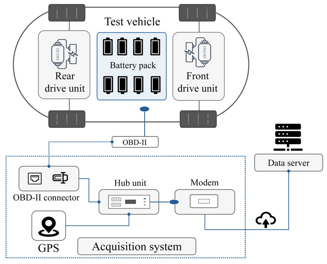
Figure 1. Architecture of the OBD-II data acquisition system.
Machines 14 01043 g001
Figure 2. Energy-flow and auxiliary energy boundary of the range-extended electric vehicle.
Machines 14 01043 g002
Figure 3. Energy consumption in pure-electric mode and range-extended mode under low-temperature conditions.
Machines 14 01043 g003
Figure 4. Effects of trip parameters on cumulative auxiliary energy consumption.
Machines 14 01043 g004
Figure 5. Effect of thermal management load level on auxiliary energy consumption.
Machines 14 01043 g005
Figure 6. Effect of range-extender operating share on auxiliary energy consumption.
Machines 14 01043 g006
Figure 7. Thermal management energy components across range-extender operating shares.
Machines 14 01043 g007
Figure 8. Correlation and multicollinearity diagnostics of candidate trip-scale variables: (a) Pearson correlation heatmap; (b) Tolerance-based multicollinearity test.
Machines 14 01043 g008
Figure 9. Feature importance analysis of the trip-scale model by SHAP values (Random Forest).
Machines 14 01043 g009
Figure 10. Grouped feature importance of the RF model based on mean absolute SHAP values.
Machines 14 01043 g010
Figure 11. Correlation and multicollinearity diagnostics of candidate second-scale variables for 20 s sample duration: (a) Pearson correlation heatmap; (b) Tolerance-based multicollinearity test.
Machines 14 01043 g011
Figure 12. The prediction accuracy R2 trends of the second-scale models across sample durations.
Machines 14 01043 g012
Figure 13. Integrated application framework of the trip-scale RF model and the 30 s LSBoost model.
Machines 14 01043 g013
Figure 14. Mean absolute errors of updated entire trip auxiliary energy predictions for the 36 trips.
Machines 14 01043 g014
Figure 15. Iterative prediction trajectories and residuals of remaining auxiliary energy consumption.
Machines 14 01043 g015
Figure 16. Trip-scale initialization and second-scale updates of total auxiliary energy consumption.
Machines 14 01043 g016
Table 1. Main parameters of the tested Li Auto L8 vehicle.
ParameterSpecificationParameterSpecification
Vehicle/modelLi Auto L8PowertrainRange-extended; dual-motor four wheel drive
Dimensions (L × W × H)5080 × 1995 × 1800 mmWheelbase3005 mm
Curb/gross mass2470–2480/3080 kgBattery42.8 kWh,
ternary lithium-ion
Front traction motor130 kW peak;
220 N·m peak torque
Rear traction motor200 kW peak;
400 N·m peak torque
Range-extender engine1.5 L, 113 kW
Sources: MIIT vehicle catalog and manufacturer information [26,27]. Manufacturer documentation confirms PTC-based cabin heating and integrated thermal management, but detailed information on Li Auto L8 subcomponents including the PTC heater, electric compressor, inverter architecture and so on is confidential and therefore cannot be publicly disclosed.
Table 2. Predictive performance of trip-scale auxiliary energy models.
DatasetMetricLSBoostRFMLP
TrainR20.978 ± 0.0100.937 ± 0.0160.827 ± 0.145
TestRMSE/kWh0.333 ± 0.0830.317 ± 0.1240.351 ± 0.134
MAE/kWh0.120 ± 0.0280.112 ± 0.0400.192 ± 0.057
R20.814 ± 0.0760.826 ± 0.1050.796 ± 0.152
Values are mean ± standard deviation. RMSE and MAE are expressed in kWh.
Table 3. Main hyperparameters and determination methods of the three trip-scale models.
ModelOptimization and ValidationSelected Configuration
LSBoostBayesian optimization;Cycles 381;
expected-improvement-plus;learning rate 0.01008176;
25 evaluations;maximum splits 97;
grouped fourfold cross-validation RMSEminimum leaf 3.
RFBayesian optimization;Trees 597;
expected-improvement-plus;minimum leaf 1;
25 evaluations;maximum splits 397;
grouped fourfold cross-validation RMSEsampled predictors 6.
MLPExhaustive grid search;
grouped fourfold cross-validation RMSE
LayerSizes 4;
λ 0.5; iterations 60.
ReLU.
Table 4. Accuracy comparison of the second-scale prediction models’ performance results across sample durations.
ModelMetricSample Duration [s]
5 s10 s15 s20 s30 s60 s
LSBoostTrain R20.8050.8550.8420.8790.9260.940
Test R20.7430.7920.8180.8400.8570.872
RMSE0.3970.3340.2980.2700.2450.210
MAE0.2890.2480.2250.2040.1830.159
RFTrain R20.7270.7910.8300.8520.8800.904
Test R20.7220.7780.8100.8250.8420.859
RMSE0.4130.3460.3040.2840.2580.221
MAE0.3100.2600.2290.2150.1950.168
MLPTrain R20.7120.7690.7940.8110.8240.836
Test R20.7110.7680.7920.8090.8220.830
RMSE0.4210.3530.3190.2960.2740.243
MAE0.3210.2700.2450.2280.2110.188
Values are means. RMSE and MAE are expressed in kW.
Table 5. Statistical errors of updated entire trip auxiliary energy predictions for holdout samples.
MetricValue (kWh)
MAE0.014
RMSE0.032
Standard deviation of absolute error0.029
90th percentile of absolute error0.030
95th percentile of absolute error0.048
Table 6. Comparison with recent studies on electric vehicle energy and auxiliary load prediction.
StudyVehiclePrediction TargetModel Framework
Schäfers
et al. [20]
BEVAuxiliary power and trip auxiliary energyAuxiliary power and trip energy predicted independently
Kim
et al. [23]
Commercial BEVTrip-based and seconds-based auxiliary energyTwo temporal scales modeled independently
Present
study
REEV under
low-temperature operation
Predict initial auxiliary energy and updatesTrip-scale RF coupled with 30 s LSBoost iterative updates
Disclaimer/Publisher’s Note: The statements, opinions and data contained in all publications are solely those of the individual author(s) and contributor(s) and not of MDPI and/or the editor(s). MDPI and/or the editor(s) disclaim responsibility for any injury to people or property resulting from any ideas, methods, instructions or products referred to in the content.