Article

A Delay-Aware Method for Inverter Nonlinearity Compensation in Sensorless PMSM Drives
1
School of Automation, Guangxi University of Science and Technology, Liuzhou 545006, China
2
College of Mechanical and Marine Engineering, Beibu Gulf University, Qinzhou 535011, China
3
School of Mechatronics Engineering, Beijing Institute of Technology, Beijing 100081, China
*
Authors to whom correspondence should be addressed.
Machines 2026, 14(9), 1041; https://doi.org/10.3390/machines14091041
Submission received: 9 August 2026 / Revised: 25 August 2026 / Accepted: 28 August 2026 / Published: 14 September 2026
(This article belongs to the Special Issue Advanced Sensorless Control of Electrical Machines)

Abstract

This paper presents a delay-aware observer-side voltage-source inverter (VSI) nonlinearity compensation chain for medium- and high-speed sensorless control of permanent magnet synchronous motors (PMSMs). The method reduces the observer-model voltage mismatch caused by inverter nonlinearities and is implemented with a continuous boundary-layer adaptive-gain sliding-mode observer (ASMO) and a second-order phase-locked loop (PLL). Two-point linear prediction estimates the phase current when the VSI nonlinear voltage error actually takes effect. A C 1 -continuous cubic zero-crossing weight limits abrupt direction changes near current zero crossings, while a synchronous correlation signal derived from the estimated back electromotive force updates the equivalent distortion-voltage amplitude online. Compensation is applied only to the reconstructed ASMO input voltage, leaving the original current loop and space-vector pulse-width modulation (SVPWM) unchanged. Comparative and ablation simulations show lower characteristic back-EMF harmonics and electrical rotor-position estimation error than conventional compensation. Hardware tests under variable-speed and load-step conditions confirm improved dynamic estimation and disturbance rejection. The intended operating region is medium to high speed, where the back-EMF has sufficient signal-to-noise ratio and a nonsalient machine model is appropriate. The fixed-point realization is reported as implementation-feasibility evidence rather than as the principal contribution.

1. Introduction

Permanent magnet synchronous motors (PMSMs) combine high efficiency and power density with fast dynamic response, making them common in servo drives, transportation, industrial automation, and compact robotic actuators. These properties are also attractive for lower-limb rehabilitation exoskeletons, whose joint drives must remain compact and reliable while providing accurate motion control. Field-oriented control (FOC) normally obtains rotor position and speed from a mechanical sensor, but the sensor adds cost, occupies installation space, and can be vulnerable to the operating environment. Sensorless control derives the same information from electrical measurements and a machine model, reducing this dependence under suitable operating conditions [1]. High-frequency injection can cover the low-speed region, although it introduces additional loss, noise, and computation. Back-EMF observers are less intrusive at medium and high speeds [2]. Accordingly, this work focuses on the back-EMF-observable region and assumes negligible motor saliency.
Sliding-mode observers (SMOs) use current-observation error to generate a switching injection and offer robust estimation with modest computational demand [1]. With a fixed gain, however, reachability at high speed and chattering at low speed impose competing requirements. A continuous boundary layer softens the switching action but introduces a phase lag that varies with speed and parameters. The adaptive-gain SMO (ASMO) and phase compensation reported in [3] address this compromise. Other studies have improved convergence or back-EMF quality through high-order, fixed-time, and quasi-super-twisting structures [4,5,6,7,8,9]. Finite-time observers and modified phase-locked loops (PLLs) have likewise been used to reduce ramp error and reject harmonics [10,11,12,13]. These observer developments generally rely on the voltage model receiving a faithful representation of the motor-terminal voltage.
The voltage applied by a practical voltage-source inverter (VSI) differs from its modulation reference because of dead time, switching delay, device voltage drops, and dc-link variation. Observer-based and recursive least-squares (RLS) approaches can estimate this distortion, whereas compensation based on a fixed inverter model remains sensitive to the operating point [14,15]. Current-dependent voltage distortion is dominated by 5th- and 7th-order components, which appear as 6 m -order position ripple after synchronous demodulation [4,16,17,18,19,20]. A fixed compensation amplitude cannot follow temperature, dc-link voltage, or device-state changes. Reducing the gain near current zero crossings limits erroneous compensation but leaves the timing mismatch unresolved [21]. RLS and harmonic-state techniques provide adaptation at the cost of covariance updates, iterations, or extra observer states [15,17,19,20,22]. A recent active-flux/MRAS method jointly adapts the position observer and corrects the PWM duty ratio online [23]. Sampling, computation, observer dynamics, and pulse-width modulation (PWM) updating introduce additional digital delay [24,25,26]. If the phase current reverses between sampling and actuation, its sampled polarity selects the wrong compensation direction, and the magnitude of the resulting compensation-voltage error can reach twice the equivalent distortion-voltage amplitude.
The principal contribution is a delay-aware observer-side compensation chain that coordinates two-point current prediction, C 1 -continuous cubic zero-crossing weighting, and online equivalent-distortion-voltage amplitude correction without modifying the current controller or SVPWM. Its organizing issue is the timing mismatch between current sampling and the actual actuation of the VSI nonlinear voltage error. Deadband, projection, and enabling logic protect the slow update when excitation or operating conditions are unsuitable. Matched comparisons among Schemes A, B, and E assess the overall effect, while the B–E ablations separate the contributions of prediction, cubic weighting, and amplitude updating. Dynamic loading, dead-time adaptation, and execution overhead are evaluated on a laboratory-developed PMSM drive. The ASMO gain law, phase compensation, and second-order PLL follow [3]; they serve as the observer baseline and are not claimed as original contributions.
Table 1 compares the present method with Refs. [4,15,16,23,24,25,26] across the five structural features relevant to this work.
Section 2 develops the PMSM and VSI-distortion models. Section 3 presents the proposed compensation method and residual-error bound. Section 4 reports the simulation and hardware results, and Section 5 concludes the paper. The analysis is local and assumes bounded residual distortion, sufficient excitation, and time-scale separation. It does not establish global asymptotic stability under saturation, loss of lock, or full-range operation.

2. System Model and Problem Formulation

2.1. Approximate PMSM Model and Sensorless FOC

For medium- and high-speed operation, a surface-mounted PMSM or another machine with negligible saliency can be represented by L d L q = L s . Parameter mismatch, weak residual saliency, and unmodeled losses are included in a bounded disturbance. The stator-current model in the stationary α β frame is
d i α β d t = R s L s · i α β + 1 L s · u α β e α β .
where R s and L s denote the stator resistance and equivalent stator inductance. The vectors i α β , u α β , and e α β are the stator current, actual equivalent terminal voltage, and back-EMF. Under the sinusoidal back-EMF assumption,
e α β = ω e ψ f sin θ e cos θ e , E = ω e ψ f .
where θ e , ω e , and ψ f are the electrical angle, electrical angular speed, and permanent-magnet flux linkage, respectively. If θ m and ω m denote the corresponding mechanical quantities and p is the number of pole pairs, then θ e = p θ m and ω e = p ω m . This study uses an amplitude-invariant Clarke transformation. The sign convention of the Park transformation is written explicitly as
i α β = C i a b c , C = 2 3 1 1 2 1 2 0 3 2 3 2 , i d q = P ( θ ^ e ) i α β , P ( θ ) = cos θ sin θ sin θ cos θ .
FOC sets i d * = 0 , while the outer mechanical-speed loop supplies the q-axis current reference i q * . Both the Park and inverse Park transformations use the estimated electrical angle θ ^ e . Only θ ^ e and ω ^ e from the ASMO-PLL close the sensorless loop; the magnetic encoder is used solely as offline ground truth. Hereafter, u α β ref is the SVPWM reference voltage and u α β is the actual equivalent motor-terminal voltage. The ASMO input u ^ α β is reconstructed from the reference voltage and estimated VSI distortion. The complete control structure is shown in Figure 1.

2.2. Adaptive-Gain SMO and Second-Order PLL

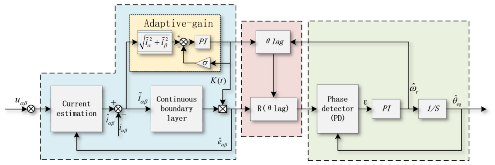
The ASMO gain law, boundary-layer phase compensation, and second-order PLL used in this subsection follow [3]. They are retained as an established observer baseline and are not original contributions of this work. With u ^ α β as its input, the continuous-boundary-layer ASMO has the current-state equation
d i ^ α β d t = R s L s · i ^ α β + 1 L s · u ^ α β z α β .
For the current-observation error e i , α β = i ^ α β i α β , equality of the observer and terminal voltages, u ^ α β = u α β , gives
L s e ˙ i , α β = R s e i , α β + e α β z α β .
Following Liu et al. [3], the continuous boundary-layer function is
f ( x ) = 1 , x a , x a , | x | < a , 1 , x a .
where a > 0 is the boundary-layer half-width. The adaptive sliding-mode gain is denoted by κ to distinguish it from the discrete sampling index. Its update law, also adopted from [3], is
δ = e i , α β 2 σ κ , κ = K p , κ δ + K i , κ 0 t δ ( τ ) d τ .
where σ is a positive proportional coefficient, and K p , κ and K i , κ are the PI gains for adaptation. The function f ( · ) acts elementwise on vectors. The sliding-mode injection and reconstructed back-EMF are
z α β = κ f e i , α β , e ^ α β z α β , a σ max | e α | , | e β | .
The final condition in Equation (8) is taken from [3] and applies under the continuous-time model and parameter assumptions used there. Within the small-error region, the boundary layer behaves as a finite-bandwidth element. The corresponding phase lag and back-EMF vector compensation are
θ lag = arctan L s ω e R s + κ / a , e ^ α β c = R ( θ lag ) e ^ α β .
PLL-based extraction remains sensitive to back-EMF harmonics and speed ramps. The trade-off between harmonic rejection and dynamic tracking is discussed in recent surveys and generalized or improved QPLL studies [10,11,12,13].
The rotation matrix is R ( θ ) = [ cos θ , sin θ ; sin θ , cos θ ] , with positive rotation defined consistently in the α β frame. The compensated vector e ^ α β c is provided to the second-order PLL, and the superscript c is omitted below. With E ^ = e ^ α 2 + e ^ β 2 , the phase-detector error and PLL states satisfy
ε θ = e ^ α cos θ ^ e e ^ β sin θ ^ e E ^ + ε E , ω ^ e = K p , θ ε θ + K i , θ ε θ d t , θ ^ ˙ e = ω ^ e .
Here, ε E > 0 is an additive regularization constant with units of volts; it prevents the normalized phase-detector denominator from approaching zero when the estimated back-EMF amplitude is small. It should be selected well below the minimum back-EMF amplitude in the enabled operating region, while remaining above the effective numerical and measurement-noise floor. The implemented value is ε E = 0.1 V . Every comparison scheme uses the same a, K p , κ , K i , κ , K p , θ , and K i , θ , so the VSI compensation branch is the only changed element. The stability result of [3] does not extend directly to a complete closed loop with discrete sampling, residual voltage error, and online amplitude updating. Section 3.3 therefore states only a residual compensation-voltage bound and its local conditions. Figure 2 summarizes the ASMO and PLL signal chain.

2.3. VSI Nonlinearity and Error Propagation

The current direction determines the voltage deviation introduced by VSI nonlinearity. The relation between the modulation reference and actual terminal voltage is
u α β = u α β ref Δ u α β inv .
where Δ u α β inv denotes the actual equivalent VSI distortion voltage. For a two-level inverter, its dominant three-phase component is approximated by
Δ u a b c inv = V inv sgn ( i a ) sgn ( i b ) sgn ( i c ) + r a b c .
where V inv is the equivalent distortion-voltage amplitude, while r a b c collects dc-link ripple, leg mismatch, and unmodeled transients. Dead time, device delays, and voltage drops provide an initial estimate and physical bounds for this amplitude:
V inv T dead + T on T off T sw V dc + V drop ( i x , V dc , T j ) .
where T sw is the PWM switching period, T j is the junction temperature, and V drop represents the device conduction-voltage drop. Observer-based and RLS-assisted compensation schemes have also modeled these nonidealities and their equivalent distortion voltage [14,15]. After removal of the common-mode component, the Clarke transformation gives the distortion in the α β frame:
Δ u α β inv = V inv C s a s b s c + r α β , s x = sgn ( i x ) .
The balanced three-phase polarity function is six-step periodic. For an individual phase,
sgn ( sin ϑ ) = 4 π h = 1 h odd sin ( h ϑ ) h .
Phase shifting and the Clarke transformation cancel zero-sequence triplen harmonics, leaving mainly positive- and negative-sequence components of order 6 m ± 1 . For the complex estimated back-EMF e ^ s = e ^ α + j e ^ β , where j 2 = 1 , the dominant harmonics can be written as
e ^ s = j E 1 e j θ e + j m = 1 E 6 m + 1 e j ( 6 m + 1 ) θ e + E 6 m 1 e j ( 6 m 1 ) θ e .
If the harmonic amplitudes remain well below the fundamental and the angular error is small, the dominant periodic position-estimation error is approximated by
e θ 1 E 1 m = 1 A 6 m sin ( 6 m θ e + φ 6 m ) .
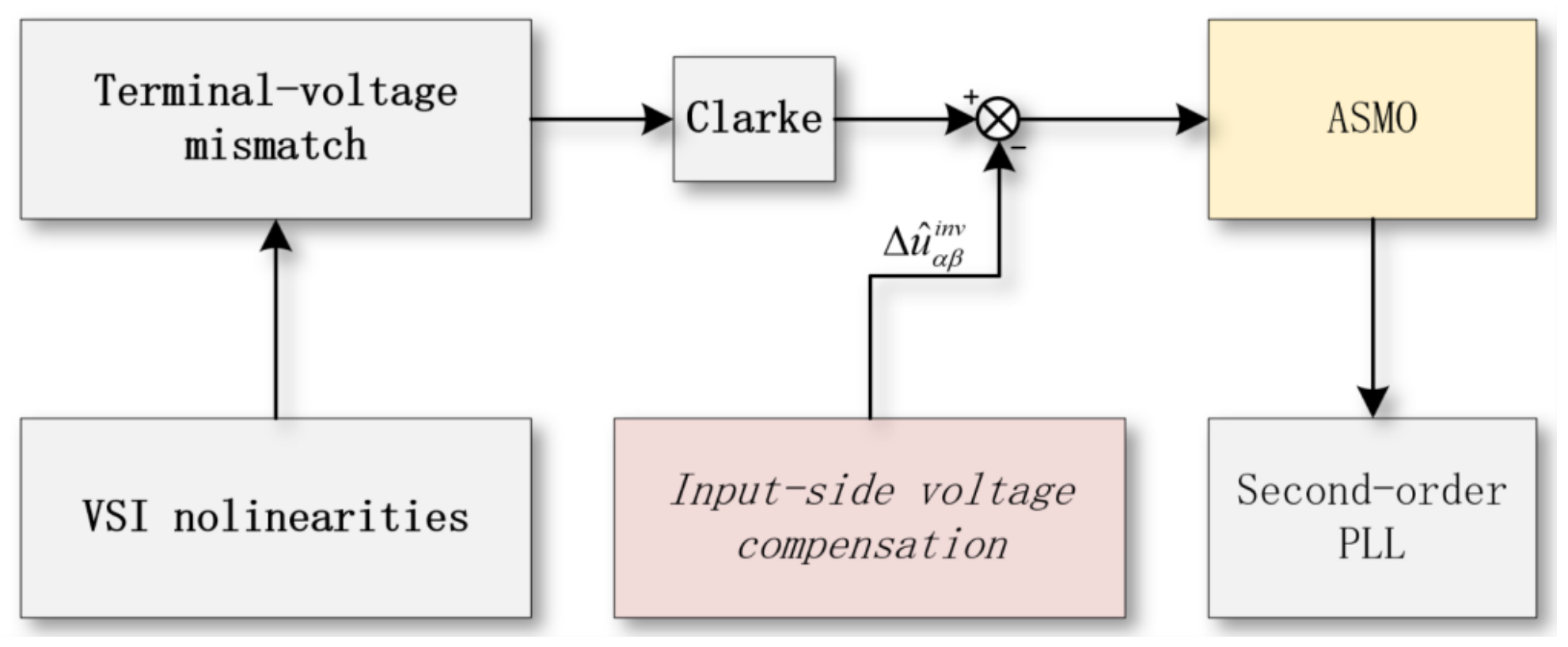
Here, E 1 > 0 is the fundamental estimated back-EMF amplitude, with units of volts, and E 6 m ± 1 are complex back-EMF harmonic coefficients containing the corresponding harmonic amplitudes and phases. The quantity A 6 m denotes the equivalent back-EMF harmonic-voltage coefficient associated with the 6 m -order electrical-position-error component and therefore has units of volts. Consequently, A 6 m / E 1 represents the corresponding small-angle electrical-position-error amplitude, which is dimensionless and expressed in radians, whereas φ 6 m denotes its phase. Thus, 5th- and 7th-order back-EMF harmonics can generate sixth-order position ripple [16,17,18,19,20]. The error e θ is the estimated electrical angle minus its reference, wrapped into ( π , π ] . In contrast to feedforward methods that alter inverter-leg commands, this work uses Δ u ^ α β inv only to reconstruct the ASMO input voltage. It directly reduces observer-model voltage mismatch; any changes in phase-current harmonics or torque ripple arise indirectly through the closed loop. Figure 3 traces this propagation path.

3. Delay-Aware VSI Nonlinearity Compensation Method

3.1. Actuation-Instant Current Prediction and C1-Continuous Cubic Zero-Crossing Weight

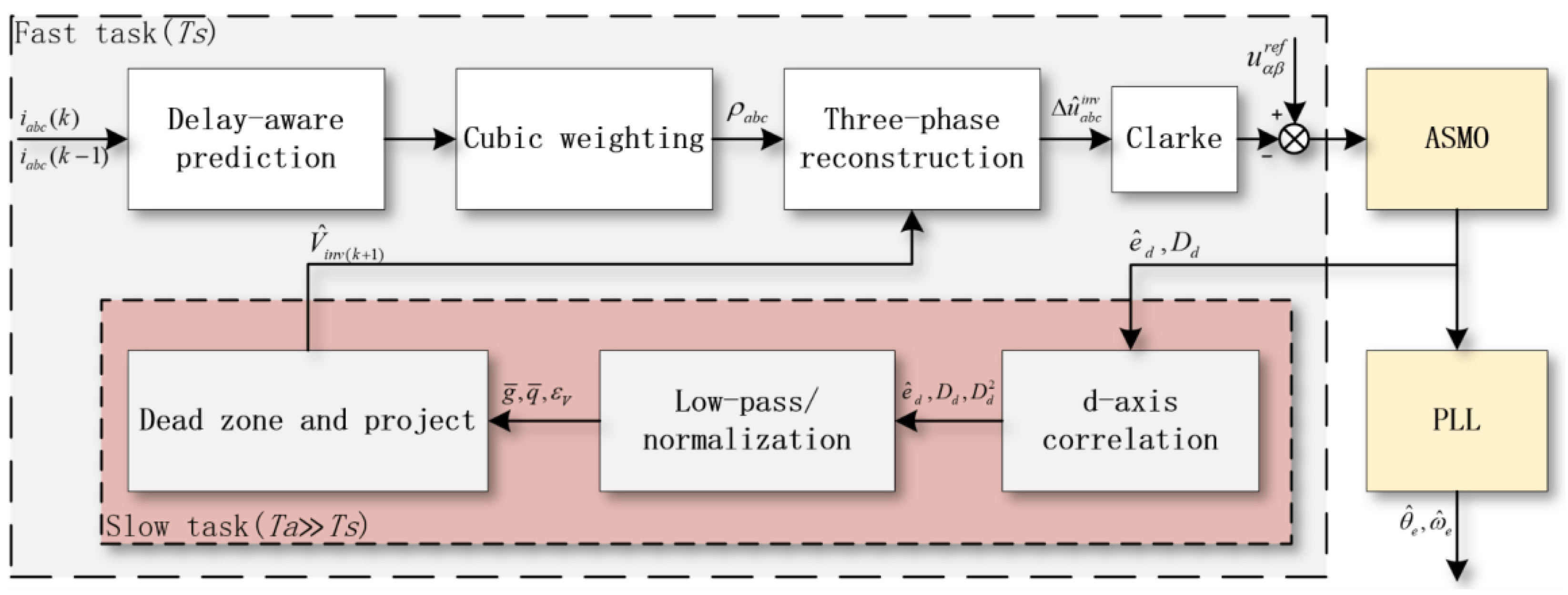
The proposed method comprises a fast current-polarity branch and a slow amplitude branch. During each current-control cycle, the fast branch predicts the phase currents at the instant when the VSI nonlinear voltage error takes effect. It then reconstructs the three-phase distortion voltage using a C1-continuous cubic zero-crossing weight. The slow branch updates the amplitude only when the observer is locked and excitation is sufficient. The equivalent digital delay from a valid ADC sample to the effective update of the new PWM duty cycle is defined as
T d = T ADC + T cal + T upd .
where T ADC , T cal , and T upd denote the sampling, computation, and PWM-update delays, respectively. Sensorless PMSM studies have reported both observer-delay suppression and overall system-delay compensation [24,25,26]. These works motivate explicit timing treatment, whereas the present method aligns the current polarity used by the observer-input VSI compensation branch through actuation-instant phase-current prediction. This delay does not mean that the observer compensation is applied directly to the inverter legs. Instead, it aligns the current polarity used for voltage reconstruction with the actual polarity at the instant when the VSI nonlinear voltage error takes effect, t k + T d . Define the actuation-instant current as i x , d = i x ( t k + T d ) , with s x , d = sgn ( i x , d ) . The conventional polarity decision is s x , 0 = sgn [ i x ( t k ) ] , yielding the following single-phase voltage error due to current-polarity misclassification:
ε u , x dir = V inv ( s x , d s x , 0 ) , ε u , x dir = 2 V inv , s x , d = s x , 0 , s x , d , s x , 0 { 1 , 1 } .
To reduce the dependence of the fast task on motor parameters, two-point linear prediction with dual saturation is used. Let i x [ k ] i x ( t k ) ; the predicted current is
i ^ x , p [ k ] = sat i x [ k ] + sat λ p ( i x [ k ] i x [ k 1 ] ) ; Δ I max , Δ I max ; I max , I max , λ p = T d T s .
where x { a , b , c } , T s is the current-sampling period, and sat ( y ; a , b ) = min { max ( y , a ) , b } . When PWM and sampling are synchronized, T s = T sw . The measured delay is T d = 100 µs, giving λ p = 1.0 . When T d T s and neither limit is active, Equation (20) reduces to 2 i x [ k ] i x [ k 1 ] .
The two saturation limits are selected from the normal operating-current range and the maximum admissible current variation during T d . Let I op , pk be the maximum normal phase-current peak, I OC the overcurrent threshold, and M I a design margin. The absolute limit is chosen to satisfy
I op , pk + M I I max < I OC .
The increment limit is selected statistically from offline current records rather than from an extreme voltage-model bound. Let Ω denote a representative calibration set that includes speed changes, load steps, and current reversals. Define
Δ I obs , max = max k , Ω , ϕ { a , b , c } i ϕ [ k ] i ϕ [ k 1 ] , Δ I req = η Δ Δ I obs , max + M Δ I , Δ I max Δ I req .
where η Δ 1 is a safety-margin factor and M Δ I is a current-measurement-noise margin obtained from ADC noise statistics. In the calibration data set Ω , the maximum normal instantaneous phase-current peak was I op , pk = 4.4 A . With M I = 1.0 A , I max = 8 A , and I OC = 9.77 A , Equation (21) is satisfied. All current limits in Equations (20)–(22) are expressed as instantaneous phase-current peak values. The offline records give Δ I obs , max = 0.72 A per sampling period; with η Δ = 1.2 and M Δ I = 0.1 A , Equation (22) gives Δ I req = 0.964 A , and the implemented increment limit is rounded upward to Δ I max = 1 A . Thus, I max prevents the predicted current from exceeding the admissible operating range, whereas Δ I max suppresses noise spikes and abnormal extrapolation. The latter is an engineering limiter calibrated from representative records; it is not a strict theoretical upper bound on PMSM current dynamics.
To reduce abrupt polarity changes caused by prediction errors and current noise in the zero-crossing region, define I th > 0 and use the following C1-continuous cubic zero-crossing weight:
ξ = i I th , ρ ( i ) = 1 , ξ 1 , ξ ( 3 ξ 2 ) 2 , | ξ | < 1 , 1 , ξ 1 .
Its first derivative is
ρ ( i ) = 3 2 I th ( 1 ξ 2 ) , | ξ | < 1 , 0 , | ξ | 1 .
Equations (23) and (24) show that ρ C 1 ( R ) , although second-derivative continuity at the boundaries is not required. We set I th = 0.2 A , above the measured current-sampling offset and noise range. The fast task sequentially updates historical samples, performs two-point linear prediction, applies saturation, evaluates ρ , and reconstructs the three-phase voltage. The current sample initializes the history at the first valid acquisition. Under overcurrent, undervoltage, abnormal sampling, or PLL loss of lock, the algorithm retains the latest valid amplitude and bypasses online updating.

3.2. Online Update of the Equivalent Distortion-Voltage Amplitude

The single-phase distortion-voltage estimate generated by the fast branch is
Δ u ^ x inv [ k ] = V ^ inv [ ] ρ i ^ x , p [ k ] , x { a , b , c } .
where k and denote the fast-sampling index and slow amplitude-update index, respectively. Let = ( k ) denote the slow-update interval containing fast sample k. V ^ inv [ ] is held constant by a zero-order hold between two successive slow updates. If one update occurs every N a fast samples, then ( k ) = k / N a . For conciseness, the discrete indices are omitted in Equations (26), (31) and (33). A fixed V ^ inv cannot accommodate changes in temperature, dc-link voltage, and device voltage drops. Online RLS and parameter-identification mechanisms can track operating-point variations but require additional recursive states [15,22]. The low-bandwidth correlation update developed here instead uses two scalar filtered statistics and a projected deadband update. For a PMSM with negligible saliency and nearly sinusoidal back-EMF, the d-axis component is nearly zero. This approximation holds when the d-axis aligns with the rotor flux and the angular error is small. To avoid confusion with update deadband operator D, φ d denotes the d-axis projection of the compensation direction:
e ^ d = e ^ α cos θ ^ e + e ^ β sin θ ^ e , φ d = cos θ ^ e sin θ ^ e C ρ ( i ^ a , p ) ρ ( i ^ b , p ) ρ ( i ^ c , p ) .
Within a local region where i d 0 , the PLL is locked, and the angular error is small, e ^ d ( V inv V ^ inv ) φ d + ν d . Here, ν d collects parameter mismatch, measurement noise, flux harmonics, the projection of unmodeled distortion r a b c , and zero-crossing smoothing bias from sgn ( i x , d ) ρ ( i x , d ) . It also includes the residual actuation-instant current-prediction error. The slow task samples only at fast indices k , so e ^ d [ ] e ^ d [ k ] and φ d [ ] φ d [ k ] . It then applies first-order low-pass updates to the correlation and excitation variables:
g ¯ [ ] = ( 1 λ a ) g ¯ [ 1 ] + λ a e ^ d [ ] φ d [ ] , q ¯ [ ] = ( 1 λ a ) q ¯ [ 1 ] + λ a φ d 2 [ ] .
where 0 < λ a < 1 .
The online amplitude-update task is executed at 100 Hz, once every 100 current-control cycles, so its update period is 10 ms. In contrast, 1 Hz is the cutoff frequency of the low-pass filter applied to the correlation variables. For the 10 ms update period, the corresponding discrete coefficient is λ a = 1 exp ( 2 π × 1 × 0.01 ) = 0.0609 . Thus, 100 Hz denotes the task execution frequency, whereas 1 Hz denotes the filter bandwidth.
The normalized correlation residual is defined as
ε V [ ] = g ¯ [ ] q ¯ [ ] + ε q .
Here ε q > 0 prevents division by zero under insufficient excitation. A symmetric update deadband is introduced to suppress noise-induced back-and-forth updates:
D ( ε ; ε n ) = 0 , | ε | ε n , ε ε n sgn ( ε ) , | ε | > ε n .
The amplitude update law is written explicitly as
V ^ inv [ + 1 ] = Π [ V min , V max ] V ^ inv [ ] + γ V D ( ε V [ ] ; ε n ) , χ [ ] = 1 , V ^ inv [ ] , χ [ ] = 0 .
Π [ V min , V max ] denotes the projection operator, and χ { 0 , 1 } is the online amplitude-update enabling variable. The implemented update uses ε q = 0.005 , ε n = 0.02 V , γ V = 0.125 , V min = 0 V , and V max = 3 V . Let h [ ] = 1 when the back-EMF amplitude exceeds 3 V, q ¯ > q min = 0.05 , the PLL is locked, the current and dc-link samples are valid, and neither the PI controller nor SVPWM has been saturated for two consecutive slow updates. Otherwise, h [ ] = 0 .
The enabling logic uses the two states INIT/HOLD ( χ = 0 ) and TRACK ( χ = 1 ). At startup, INIT/HOLD is retained for N init = 10 slow updates (0.10 s). A reversal trigger is generated from the sign change of the q-axis current reference:
r rev [ ] = 1 , i q * [ ] i q * [ 1 ] < 0 , 0 , otherwise .
If r rev = 1 or h = 0 , the state enters HOLD immediately. A reversal HOLD lasts at least N H = 16 slow updates (0.16 s). TRACK resumes only when this interval has elapsed and h = 1 , | i q | I q , rel = 0.30 A , and sgn ( i q ) = sgn ( i q * ) for N rel = 2 consecutive slow updates. The separation between I th = 0.20 A and I q , rel = 0.30 A provides 0.10-A release hysteresis. Equation (30) leaves the stored amplitude register unchanged whenever χ = 0 . Any nonzero displayed difference is limited to readout or plotting quantization. Parameters λ a and γ V keep the amplitude-update bandwidth substantially below the current-loop, ASMO, and PLL bandwidths. Thus, V ^ inv follows only slow device-state variations and does not track harmonics within each PWM cycle.

3.3. Compensation Integration and Supporting Analyses

The zero-sequence component is first removed from the three-phase distortion estimate, which is then transformed into the α β coordinates:
Δ u ^ a b c inv = V ^ inv ρ ( i ^ a , p ) ρ ( i ^ b , p ) ρ ( i ^ c , p ) , Δ u ^ α β inv = C Δ u ^ a b c inv Δ u ^ 0 inv 1 3 .
where Δ u ^ 0 inv = ( Δ u ^ a inv + Δ u ^ b inv + Δ u ^ c inv ) / 3 and 1 3 = [ 1 , 1 , 1 ] T . The reconstructed ASMO input voltage and the general current-error equation are
u ^ α β = u α β ref Δ u ^ α β inv , L s e ˙ i , α β = R s e i , α β + e α β + Δ u ˜ α β inv z α β .
where Δ u ˜ α β inv = Δ u α β inv Δ u ^ α β inv = u ^ α β u α β .
The following propositions are supporting analyses for the engineering compensation method. They characterize a residual-voltage-error bound and a local contraction condition, respectively, and are not a general closed-loop stability theorem.
Proposition 1
(supporting residual voltage-error bound). Let i x , d = i x ( t k + T d ) , e p , x = i ^ x , p [ k ] i x , d , and V ˜ inv = V inv V ^ inv . If | r x | r max and 0 V inv , V ^ inv V max , the single-phase residual satisfies
Δ u x inv Δ u ^ x inv r max + V max b ρ , x + V ˜ inv + 3 V max 2 I th e p , x .
where b ρ , x = | sgn ( i x , d ) ρ ( i x , d ) | .
Proof. 
Add and subtract V ^ inv ρ ( i x , d ) , apply the triangle inequality, and use | ρ | 1 together with | ρ ( i ^ x , p ) ρ ( i x , d ) | 3 | e p , x | / ( 2 I th ) . □
Proposition 2
(supporting local amplitude-error contraction). Assume that the true amplitude is approximately constant between two slow updates, the enabling variable equals 1, and the projection and update deadband are inactive. Under the local linearization that neglects the correlated disturbance term, Equations (27)(30) give
V ˜ inv [ + 1 ] 1 γ V q ¯ [ ] q ¯ [ ] + ε q V ˜ inv [ ] .
The amplitude error contracts successively in this local scalar model if
0 < γ V q ¯ [ ] q ¯ [ ] + ε q < 2 .
Proof. 
The multiplier in Equation (34) has magnitude below one exactly when Equation (35) holds. □
Proposition 1 separates the effects of unmodeled voltage, zero-crossing bias, amplitude-estimation error, and prediction error. Proposition 2 further assumes sufficient excitation, bounded residual input, and time-scale separation between the amplitude update and observer dynamics. It is a local contraction result, not a global stability proof for the complete discrete-time drive.

3.4. Real-Time Implementation

The fixed-point realization on the LCM32F039 is reported only as implementation-feasibility evidence. The fast compensation branch executes synchronously with the 10 kHz current loop, while the amplitude update is evaluated at 100 Hz. V ^ inv is held constant between successive slow-task updates. The resulting real-time implementation is shown in Figure 4.

4. Simulation and Experimental Results

4.1. Simulation Setup, Experimental Platform, and Evaluation Metrics

MATLAB R2025a simulations used a 0.1 ms controller sampling period and the same data-recording interval. An averaged nonlinear VSI model represented dead time through an equivalent voltage error, and a discrete block imposed the digital delay. PMSM parameters, current-loop, ASMO and PLL settings, sampling frequency, and data processing were identical across all schemes. Only the VSI nonlinearity-compensation branch changed between comparisons.
Five progressive schemes were evaluated. Scheme A had no VSI nonlinearity compensation. Scheme B combined currently sampled phase currents, a linear zero-crossing weight, and a fixed equivalent distortion-voltage amplitude. Scheme C changed only the current input of Scheme B to the predicted phase currents. Scheme D retained the fixed amplitude but replaced the linear weight with the C1-continuous cubic weight. Adding online amplitude updating to Scheme D produced the complete Scheme E. The fixed-amplitude setting was identical in Schemes B–D.
Steady-state tests compared Scheme A, conventional Scheme B, and complete Scheme E. Delay sensitivity and module ablation were examined with Schemes B–E. The B-to-C, C-to-D, and D-to-E comparisons isolated prediction, cubic weighting, and online amplitude updating, respectively. The 600 1500 600 r / min command used linear ramps. Acceleration was 1000 r/min/s with 1 s plateaus, while deceleration was 650 r/min/s with 1.5 s plateaus.
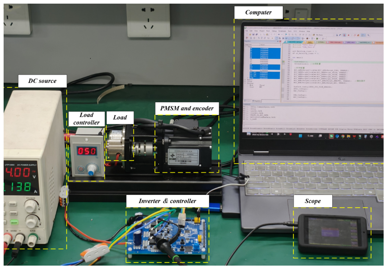
Hardware tests used the in-house PMSM drive platform in Figure 5. It comprised a dc supply, a two-level VSI, an LCM32F039 control board, a 200 W PMSM, a magnetic encoder, and a 1 N · m magnetic powder brake. The brake provided adjustable load torque. The encoder recorded rotor position and speed for offline error evaluation only and was excluded from the sensorless loop. Table 2 lists the principal platform and control parameters.
The permanent-magnet flux linkage in Table 2 was remeasured as ψ f = 0.0166 Wb . Using Equation (2), the corresponding back-EMF amplitudes are 5.22 V at 600 r/min and 13.04 V at 1500 r/min. For the 24 V dc link, the linear-SVPWM phase-voltage limit is V dc / 3 = 13.86 V ; hence, the 1500-r/min point has a back-EMF-only voltage headroom of approximately 0.82 V, corresponding to an ideal modulation ratio of 0.941 before stator and inverter voltage drops are included. All reported hardware tests are confined to the 600–1500 r/min mechanical-speed range, and no operation above 1500 r/min is claimed.
The comparison with Ref. [16] is a module-level controlled benchmark. Its RTLS-based equivalent-distortion-amplitude estimator was transplanted into the common ASMO–PLL platform, while the motor, current and speed controllers, sampling and PWM settings, dead time, effective delay, operating condition, and evaluation windows were kept identical to those of Schemes B and E. Only the VSI nonlinearity-compensation branch was replaced; this benchmark is not presented as a complete reproduction of the sensorless architecture in Ref. [16].
The RTLS forgetting factor was set to λ = 0.998 , with P r = diag ( 1 , 1000 ) , k p , RTLS = 1 , k i , RTLS = 20 , and an LPF angular cutoff frequency of ω LPF = 461.8 rad / s . The initial equivalent distortion-voltage amplitude was set to V ^ inv ( 0 ) = 0.60 V . The RTLS-based benchmark was executed at the same 10 kHz PWM/current-loop frequency used by the other two schemes.
The encoder mechanical angle θ m , enc was converted to the electrical angle as θ e , enc [ k ] = wrap ( π , π ] ( p θ m , enc [ k ] ) , where p is the number of pole pairs. The estimated and encoder sequences used a common sampling trigger. The encoder sequence was corrected for a fixed one-sample delay. The mechanical-speed estimation error was defined as e n [ k ] = n ^ m [ k ] n m , enc [ k ] , and the electrical-position estimation error was e θ [ k ] = wrap ( π , π ] ( θ ^ e [ k ] θ e , enc [ k ] ) . The steady-state electrical-position estimation error was characterized by its peak-to-peak value. All position-error angles are reported in electrical degrees, whereas all speeds in r/min are mechanical speeds. Total harmonic distortion (THD) was defined as THD 2 : 20 ( x ) = h = 2 20 X h 2 / X 1 × 100 % , where X h is the hth-harmonic amplitude of signal x. Unless otherwise stated, fast Fourier transform (FFT) analysis was applied to the estimated back-EMF e ^ α . A continuous window of 10 electrical periods after steady state was selected. A 1200-point Hann window was used, followed by zero-padding to a 4096-point FFT. The 5th and 7th harmonics were normalized to the fundamental amplitude. The peak value of the sixth-order electrical-position-error component was reported in electrical degrees. Dynamic operating conditions reported the maximum absolute mechanical-speed estimation error and maximum dynamic electrical-position estimation error. Load-step tests reported the maximum mechanical-speed drop, maximum absolute mechanical-speed estimation error, and recovery time. Recovery time was defined as the time required for the response to re-enter ± 2 % of the reference and remain there continuously for 50 ms. Three load-step records were evaluated for each method. Individual observations and the mean ± standard deviation (SD) were reported. For visualization, the encoder-speed trajectories were processed using a 45-ms moving-average window, whereas the error trajectories used a 30-ms moving-average window. The summary metrics were calculated separately for each record before aggregation.

4.2. Simulation Verification

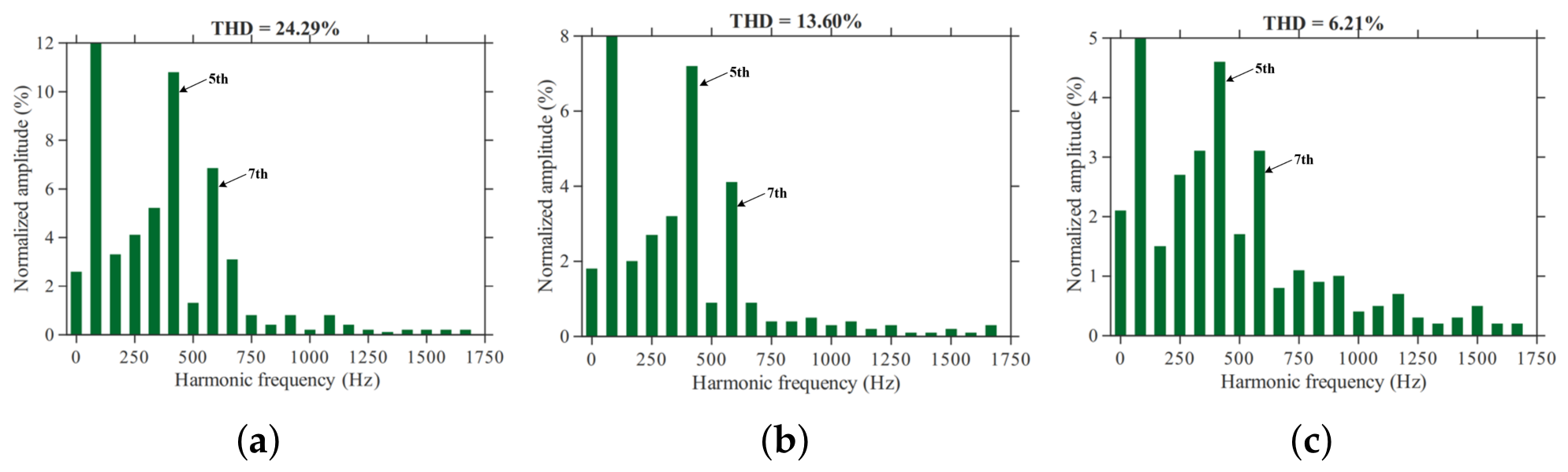
Schemes A, B, and E were compared at 1000 r/min mechanical speed, 1 µs dead time, and 10 kHz sampling. Figure 6 presents the three schemes from left to right. With the common FFT window and THD 2 : 20 definition, their THD values were 24.29%, 13.60%, and 6.21%, respectively. Relative to conventional Scheme B, complete Scheme E reduced the 5th- and 7th-harmonic amplitudes by 39.72% and 29.27%. The electrical-position-error peak-to-peak value fell from 7.82 to 4.73 , and its sixth-order component decreased by 49.73%. Table 3 collects these metrics. The A–B–E comparison measures the overall change from no compensation to the complete method; the following B–E ablation separates the individual modules. The observed harmonic changes agree with Equations (15)–(17), which link 6 m ± 1 voltage harmonics to 6 m -order electrical-position error.
Delay-sensitivity and ablation simulations used equivalent digital delays of 0, 1.0, and 1.5 sampling periods. Schemes B and C differed only in the current instant used for compensation direction. The C-to-D change was the zero-crossing weight, and the D-to-E change was online amplitude updating. Schemes B–D shared one fixed amplitude; every other control parameter and data window remained unchanged. Figure 7 includes the error trajectories needed for these comparisons without repeating four complete waveform sets.
At one sampling period of equivalent delay, Scheme B had a 16.22% current-polarity misclassification rate. Actuation-instant prediction lowered this rate to 6.10% in Scheme C. Replacing the linear weight with the C1-continuous cubic weight then reduced the maximum compensation-voltage deviation from 0.339 V to 0.254 V. From Scheme C to D, the electrical-position-error peak-to-peak value and sixth-order component decreased by 13.40% and 16.80%, respectively. Online updating in Scheme E reduced the steady-state amplitude error from 0.116 V to 0.015 V relative to Scheme D. The same comparison reduced the electrical-position-error peak-to-peak value from 4.21 to 3.44 , isolating the amplitude-update contribution. With a delay mismatch of 1.5 sampling periods, Scheme E’s dual saturation kept the maximum compensation deviation within 1.941 V. Table 4 summarizes the single-variable comparisons.
The sampled phase-a current was modeled as i a , m [ k ] = i a , d [ k ] + b a + n a [ k ] , where n a [ k ] N ( 0 , σ i 2 ) . The direction-proxy RMS error was defined as
E p = 1 N k = 1 N ρ i ^ a , p [ k ] ; I th sgn i a , d [ k ] 2 .
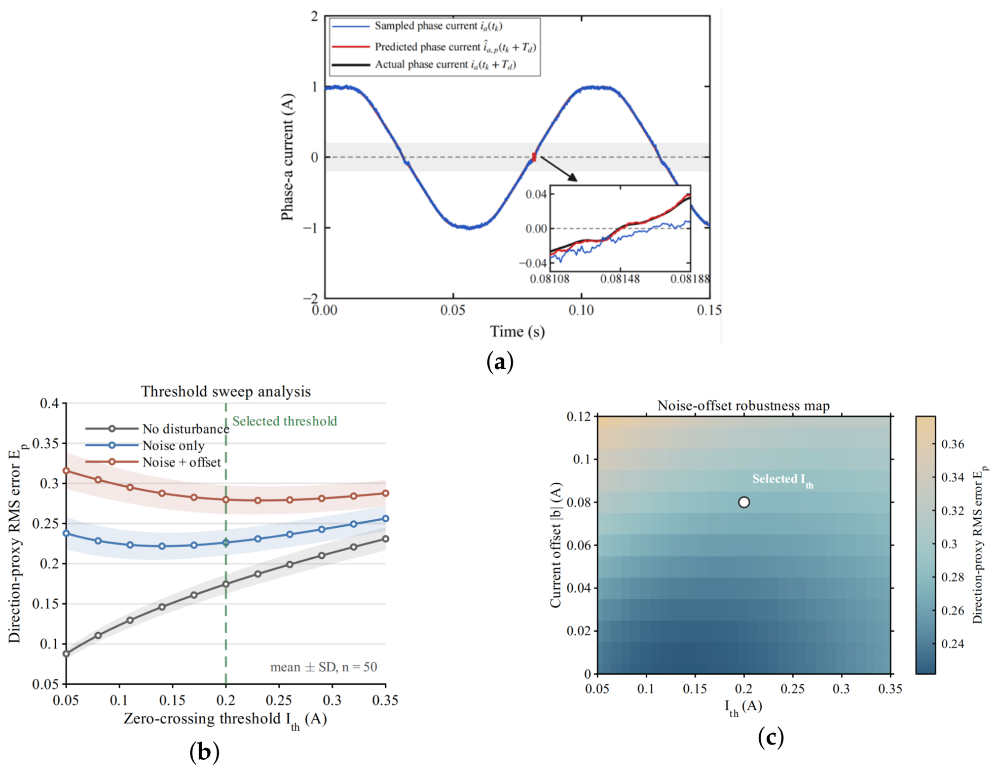
The injected noise used σ i = 0.03 A , and the noise-plus-offset case used | b a | = 0.08 A . At 10 kHz, each threshold used the same 50 realizations generated with the fixed MATLAB R2025a setting rng(1202,‘twister’). To support the selection of I th = 0.2 A , Figure 7b sweeps the threshold from 0.05 to 0.35 A under no-disturbance, noise-only, and noise-plus-offset conditions, with the direction-proxy RMS error reported as the mean ± standard deviation over 50 runs. A small threshold is favorable without disturbance but is more sensitive to noise and offset, whereas an excessively large threshold widens the smoothed zero-crossing region and increases the error. The noise-offset map in Figure 7c confirms the same trade-off over the tested offset range. The selected value of 0.2 A lies near the low-error region under the disturbed conditions without excessively widening the zero-crossing interval.
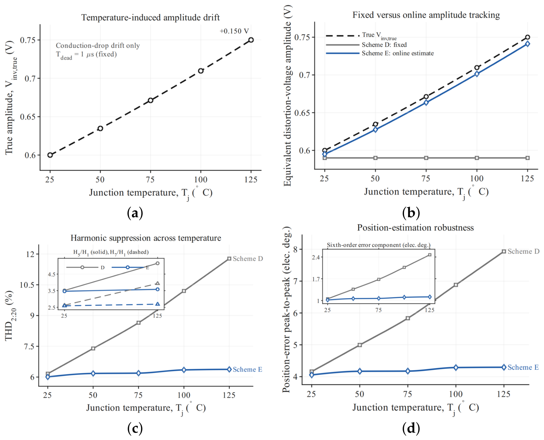
The temperature-parameterized simulation in Figure 8 externally schedules temperature from 25 to 125 °C and prescribes an increase in the equivalent VSI distortion-voltage amplitude from 0.60 to 0.75 V to emulate slow device-conduction-drop drift. Scheme D retains a fixed compensation amplitude of approximately 0.59 V, whereas the online estimate in Scheme E follows the imposed amplitude change. Consequently, the reported THD 2 : 20 rises from approximately 6.1% to 11.8% for Scheme D but remains between approximately 6.0% and 6.4% for Scheme E. The electrical-position-error peak-to-peak value similarly increases from approximately 4.1 to 7.9 with fixed compensation, while remaining near 4.0– 4.3 with the online update. This test evaluates adaptation under a prescribed temperature-dependent drift scenario; it is not an exact electrothermal model of a specific switching device.
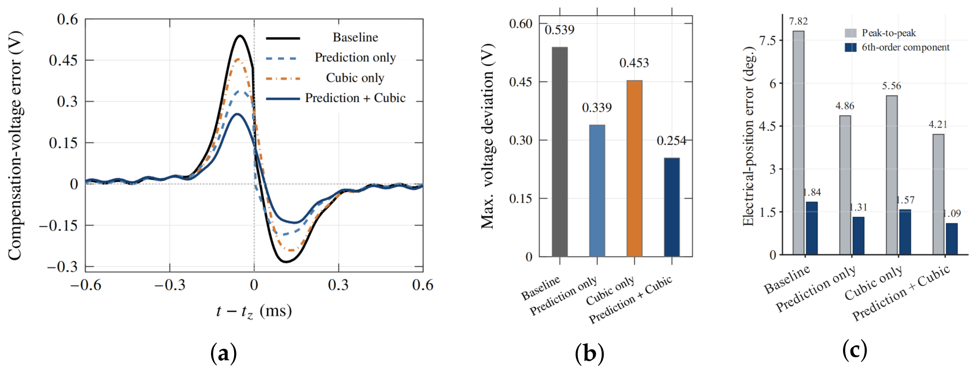
The factorial ablation in Figure 9 uses four matched groups: Baseline, Prediction only, Cubic only, and Prediction+Cubic. Prediction alone reduces the maximum compensation-voltage deviation from 0.539 to 0.339 V, whereas cubic weighting alone reduces it to 0.453 V. Their combination gives the lowest deviation of 0.254 V. The corresponding electrical-position-error peak-to-peak values are 6.52 , 4.86 , 5.56 , and 4.21 , and the sixth-order components are 1.84 , 1.31 , 1.57 , and 1.09 , respectively. Thus, prediction provides the larger individual reduction under this condition, while cubic weighting gives an additional reduction when combined with prediction. Figure 9 is a separate 2 × 2 factorial-ablation data set; its Baseline is matched only to the other three groups within that factorial comparison. It is not the Scheme-B record used in the independent A/B/E steady-state comparison of Figure 6 and Table 3. The two data sets and their peak-to-peak values are therefore reported separately and are not cross-combined.
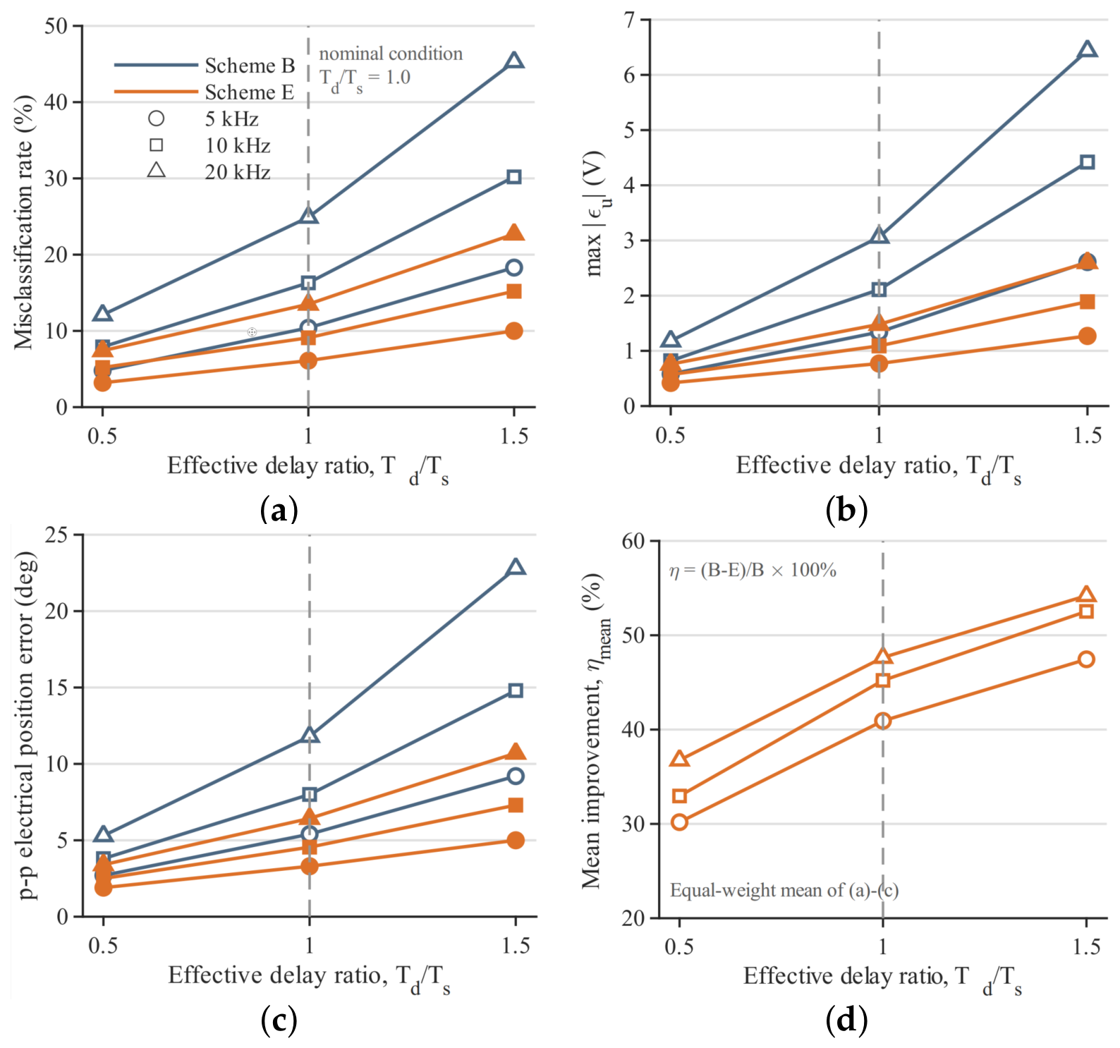
Figure 10 evaluates delay-frequency robustness at switching frequencies of 5, 10, and 20 kHz and delay ratios T d / T s = 0.5 , 1, and 1.5. Although the polarity-decision, compensation-voltage, and electrical-position errors increase as T d / T s increases, Scheme E remains below Scheme B at every tested frequency and delay ratio. The improvement ratio is defined as η = ( B E ) / B × 100 % for each metric, and Figure 10d reports their equal-weight mean. The resulting mean improvement remains positive over all nine operating combinations and is approximately 30–55%, supporting robustness to the tested switching-frequency and effective-delay variations.

4.3. Experimental Validation

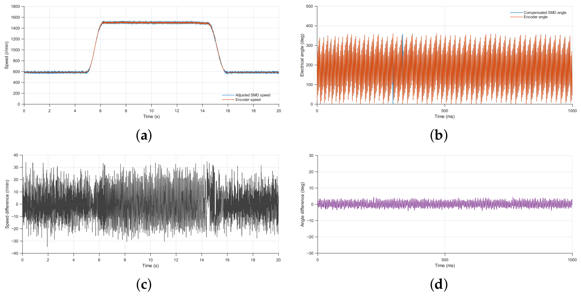
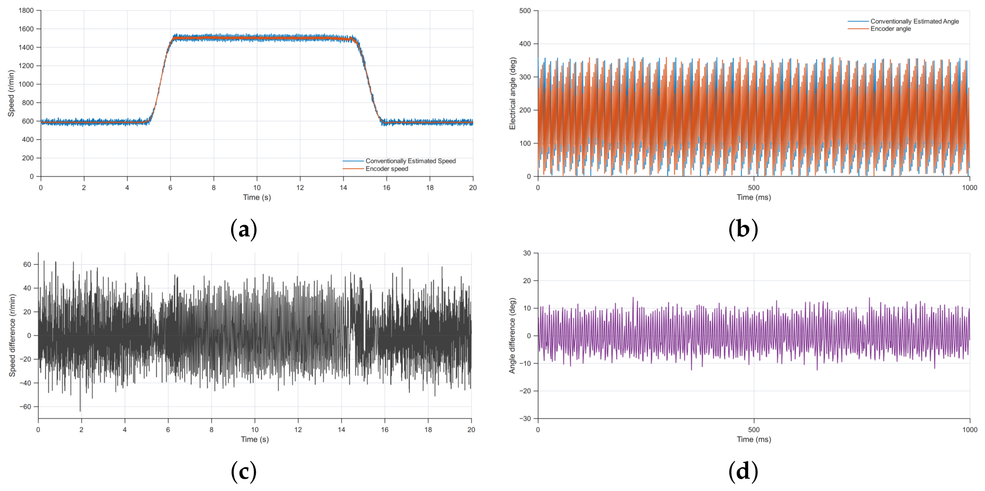
The variable-speed test followed a 600 1500 600 r / min mechanical-speed command. With identical acceleration and deceleration slopes, the maximum absolute mechanical-speed estimation errors were 62.40 r/min for Scheme B and 34.1 r/min for Scheme E. Their corresponding maximum dynamic electrical-position errors were 14.86 and 5.13 . After each speed-plateau transition, Scheme E returned to within ± 2 % of the reference within 194 ms and remained there for 50 ms. Figure 11 and Figure 12 show the hardware waveforms for Schemes B and E, respectively.
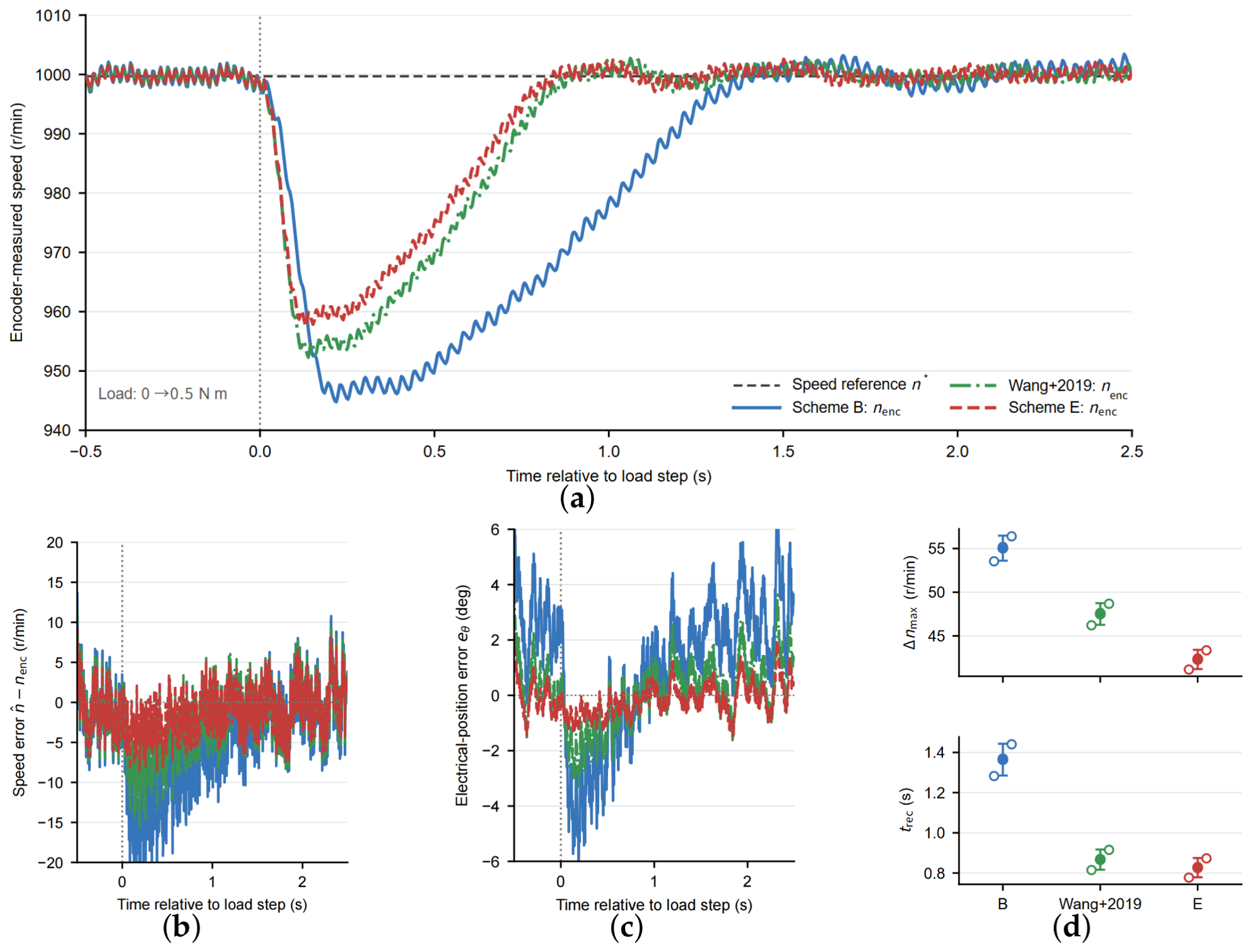
The module-level controlled load-disturbance benchmark in Figure 13 was conducted at 1000 r/min mechanical speed with a 0 0.5 N · m load step. It compared Scheme B, the transplanted RTLS compensation module from Ref. [16], and Scheme E under matched platform and controller settings. The maximum mechanical-speed drops (mean ± SD, n = 3 ) were 55.04 ± 1.43 , 47.51 ± 1.24 , and 42.30 ± 1.10 r/min, respectively. The corresponding recovery times were 1.364 ± 0.079 , 0.867 ± 0.050 , and 0.827 ± 0.048 s. Relative to Scheme B, Scheme E reduced the mean maximum speed drop by 23.15% and the mean recovery time by 39.40%. Relative to the Ref. [16] module, the corresponding reductions were 10.95% and 4.62%. Figure 13a–c show the encoder-measured speed, mechanical-speed estimation error, and electrical-position estimation error. Figure 13d summarizes the maximum speed drop and recovery time across the three records. Scheme E showed the smallest load-induced speed drop and the shortest mean recovery time. These results compare the compensation modules on the common platform and do not imply a full reproduction of Ref. [16].
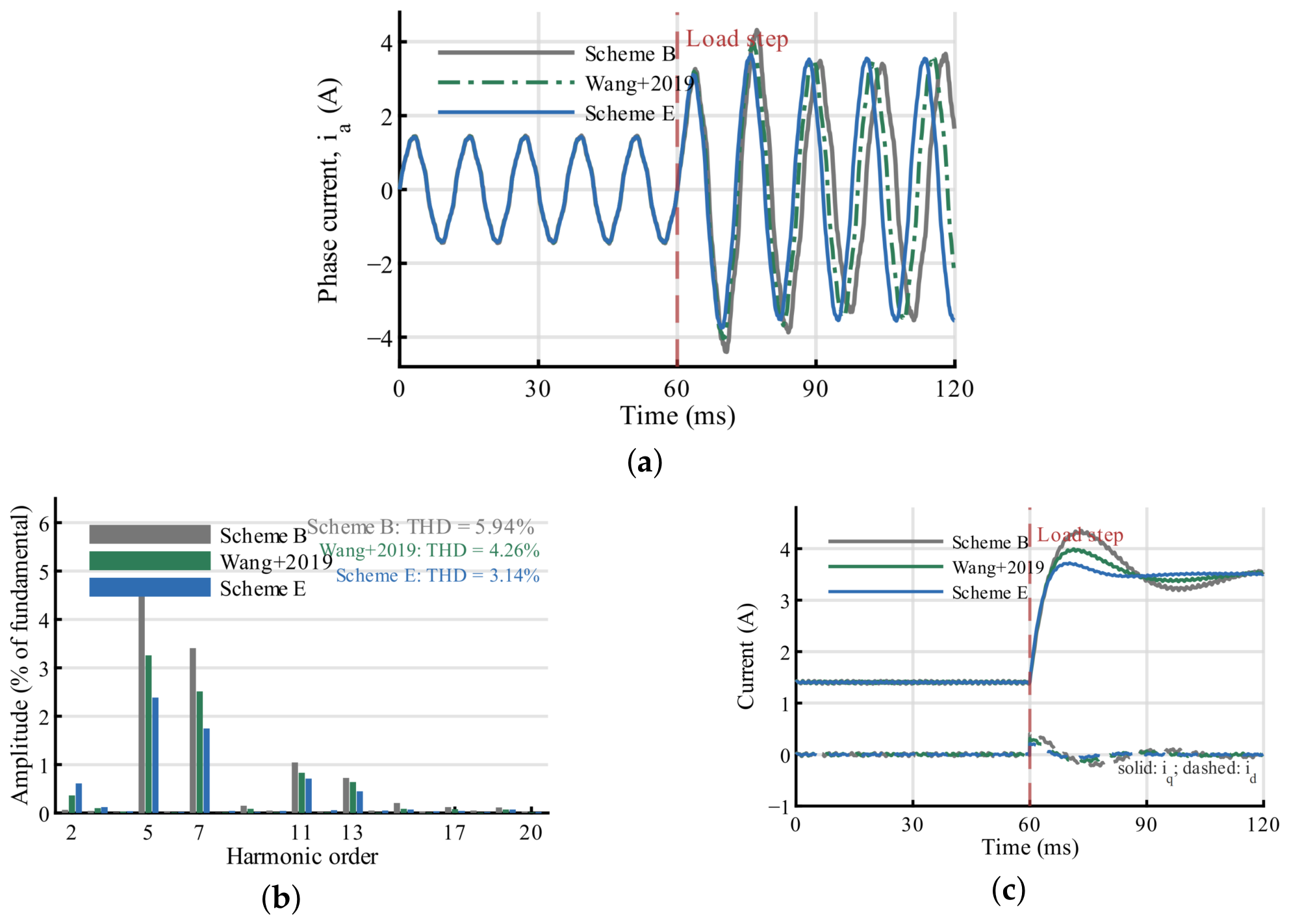
Figure 14a–c extend the same module-level benchmark with the phase-current waveform, phase-current spectrum, and d- and q-axis current responses. The displayed phase-current THD 2 : 20 values are 5.94%, 4.26%, and 3.14% for Scheme B, the Ref. [16] module, and Scheme E, respectively. The corresponding d-q responses show the same ordering: Scheme B has the largest transient i q overshoot and i d excursion, the Ref. [16] module is intermediate, and Scheme E has the smallest transient deviation. Because compensation is applied to the observer-side reconstructed voltage, these current-quality differences are interpreted as indirect closed-loop consequences of improved electrical-position estimation rather than as direct current-harmonic or torque control. No torque measurement is claimed.
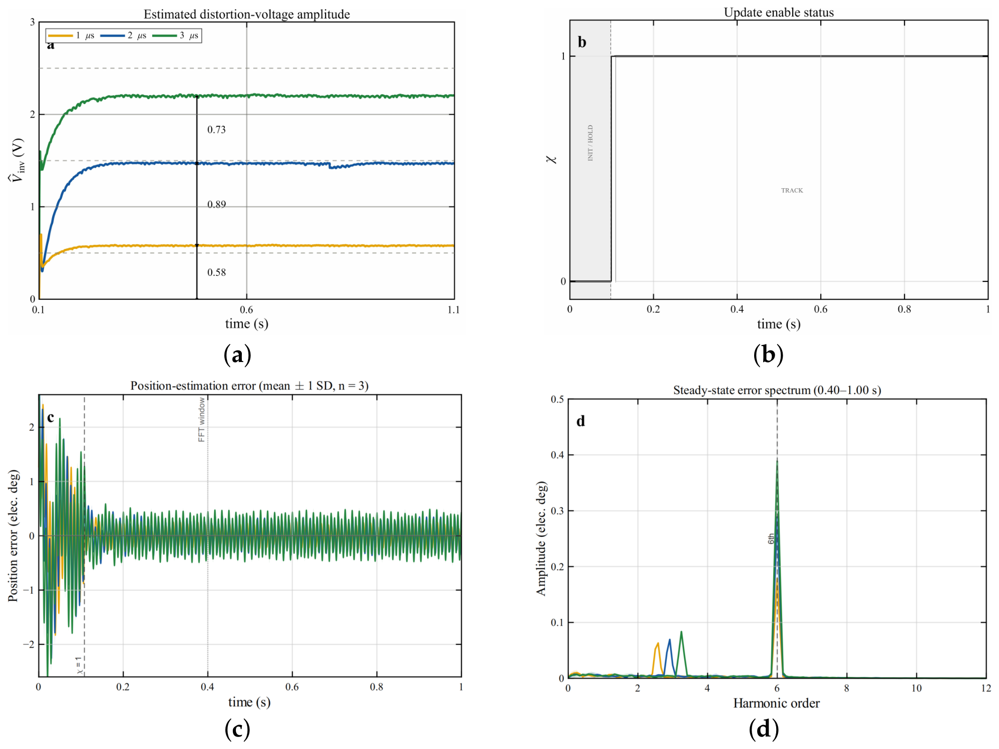
Dead-time adaptation was tested at 1 µs, 2 µs, and 3 µs. The state machine remains in INIT/HOLD during the first 0.10 s, as shown in Figure 15b. Figure 15a begins when TRACK is enabled, and its time labels include this 0.10 s initialization offset. The amplitude transients in Figure 15a therefore occur only while χ = 1 . The steady-state means of V ^ inv in Scheme E were 0.58 V, 1.47 V, and 2.20 V, respectively. Figure 15 also reports the electrical-position errors and their steady-state spectra over repeated tests. These measures characterize adaptation across the three dead times.
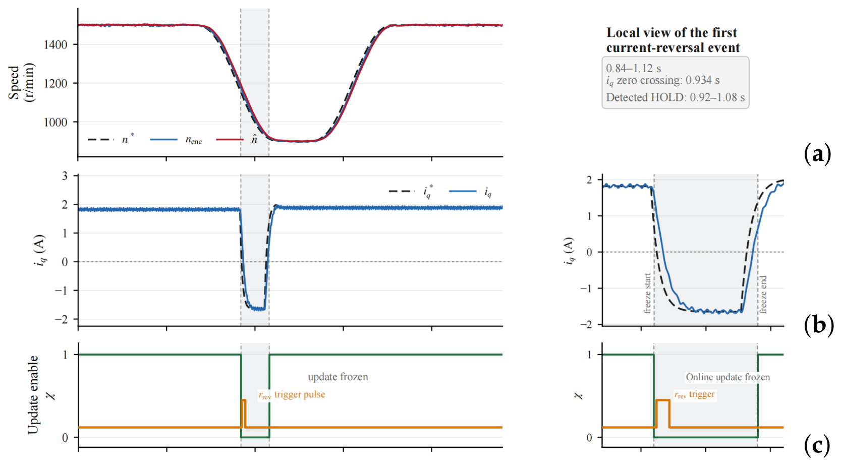
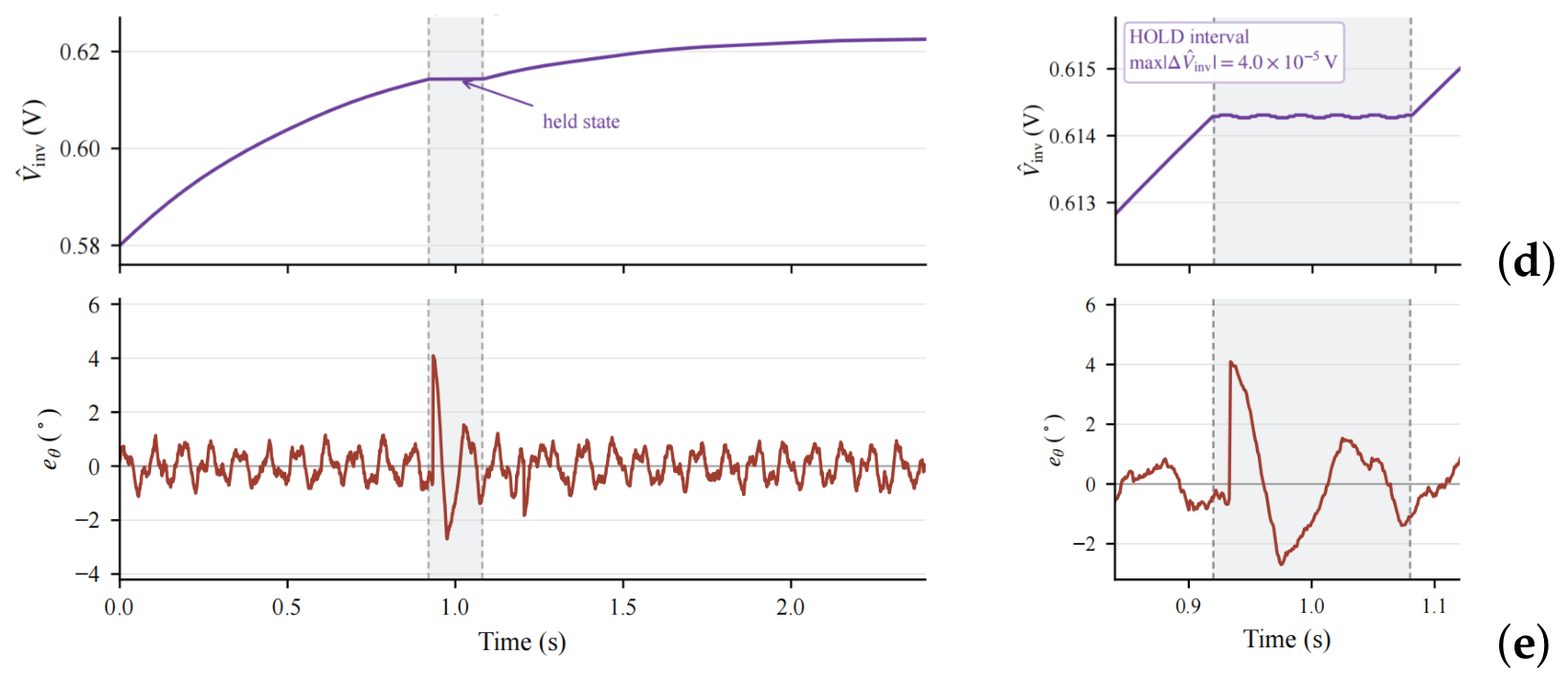
The 10-kHz hardware record in Figure 16 uses a 1500 900 1500 r / min mechanical-speed command. During the first deceleration, i q * changes from approximately + 1.8 to 1.6 A and then returns to its positive level. Its sign change generates the r rev pulse near 0.920 s and latches HOLD, so χ = 0 . The measured i q first crosses zero at approximately 0.934 s. After the 0.16 s minimum HOLD interval, the current-release and health conditions are satisfied at approximately 1.080 s. The state then returns to TRACK, χ = 1 , and online updating resumes. During HOLD, V ^ inv remains near 0.6143 V, and the displayed maximum sample-to-sample change is 4.0 × 10 5 V . The electrical-position estimation error remains bounded, with transient extrema of approximately + 4.0 and 2.8 . It returns to approximately ± 1.0 after the reversal. The hardware current-reversal test was repeated three times; Figure 16 shows one representative record.

4.4. Discussion

The method acts on the reconstructed ASMO input u ^ α β rather than the physical VSI terminal voltage. Any reduction in phase-current THD or torque ripple is therefore an indirect closed-loop consequence of improved electrical-position estimation. Unlike RLS-based inverter or motor-parameter identification [15,22] and iterative harmonic optimization [17], the implementation stores no covariance matrix and solves no iterative problem. Ref. [23] jointly changes the active-flux observer and applies MRAS-based correction to the PWM duty ratio, whereas the present chain retains the common ASMO–PLL and PWM command path. The fast branch evaluates three scalar prediction, weighting, and voltage-reconstruction paths followed by zero-sequence removal and one Clarke transformation. The two scalar filters and projected amplitude update execute only at 100 Hz. Its additional worst-case execution time on the LCM32F039 was 6.52 µs, or 6.52% of the current-control period. Flash and RAM increased by 1536 bytes and 96 bytes, respectively. These implementation results support real-time feasibility but are not presented as the main contribution.
Applicability is limited by back-EMF observability, calibrated effective delay, and synchronous excitation. The local relation in Equation (26) fails at zero or extremely low speed, during PLL loss of lock, or under sustained VSI saturation. It is also invalid for q ¯ q min or rapid current reversal, when the enabling logic freezes the update. Parameter mismatch, saliency, and flux harmonics can also leak into e ^ d . The conclusions therefore concern the tested PMSM at medium-to-high speed, where L d L q is a reasonable approximation. Zero-speed operation, strongly salient machines, and operation with large uncalibrated delay errors are outside the present scope. In addition, Figure 8 is a temperature-parameterized simulation with an externally prescribed distortion-voltage drift, not a calibrated electrothermal model or a substitute for temperature-controlled hardware validation.

5. Conclusions

This study presents a delay-aware observer-side compensation chain that coordinates two-point current prediction, C 1 -continuous cubic zero-crossing weighting, and online equivalent-distortion-voltage amplitude correction without modifying the current controller or SVPWM. The supporting analyses in Propositions 1 and 2 characterize the residual-voltage-error bound and the local contraction condition of the slow amplitude update under their stated assumptions; they do not constitute a general closed-loop stability theorem.
Against conventional compensation in the A/B/E steady-state simulation, the electrical-position-error peak-to-peak value decreased from 7.82 to 4.73 , a reduction of 39.51%. The 5th- and 7th-harmonic amplitudes fell by 39.72% and 29.27%, while the sixth-order electrical-position-error component decreased from 2.777 to 1.396 , a reduction of 49.73%. In the variable-speed hardware test, the maximum absolute mechanical-speed estimation error decreased from 62.40 to 34.1 r/min, and the maximum dynamic electrical-position error decreased from 14.86 to 5.13 . Under the 1000-r/min, 0 0.5 N · m load step, the mean maximum mechanical-speed drop decreased from 55.04 to 42.30 r/min. The mean recovery time decreased from 1.364 to 0.827 s. These changes correspond to reductions of 23.15% and 39.40%, respectively. Across the three dead times, the steady-state means of V ^ inv were 0.58 V, 1.47 V, and 2.20 V. The added fast task required 6.52 µs in the worst case, equal to 6.52% of the current-control period.
The method is limited to the medium- and high-speed region where the back-EMF remains observable. It also depends on calibrated effective delay, and the online amplitude update is frozen during rapid current reversal, persistent current saturation, loss of lock, or protection states. The temperature-parameterized simulation evaluates a prescribed slow drift and does not replace chamber- or junction-temperature-controlled hardware validation.

Author Contributions

Conceptualization, W.Z. and X.G.; methodology, W.Z.; software, W.Z.; validation, W.Z., Z.G., Y.Y., Y.G., Z.H. and P.Z.; formal analysis, W.Z.; investigation, W.Z.; data curation, W.Z.; writing—original draft preparation, W.Z.; writing—review and editing, W.Z., Z.G., Y.Y., Y.G., Z.H., P.Z. and X.G.; visualization, W.Z.; supervision, X.G.; project administration, X.G. All authors have read and agreed to the published version of the manuscript.

Funding

This research received no external funding.

Institutional Review Board Statement

Not applicable.

Informed Consent Statement

Not applicable.

Data Availability Statement

The data presented in this study are available from the corresponding author upon reasonable request.

Conflicts of Interest

The authors declare no conflicts of interest.

References

  1. Zuo, Y.; Lai, C.; Iyer, K.L.V. A Review of Sliding Mode Observer Based Sensorless Control Methods for PMSM Drive. IEEE Trans. Power Electron. 2023, 38, 11352–11367. [Google Scholar] [CrossRef] [Scilit]
  2. Franko, A.; Takáč, B.; Makyš, P. Investigation of Sensorless Control of Permanent Magnet Synchronous Motors Using Different Strategies in Mid- and High-Speed Region. Electr. Eng. 2025, 107, 10725–10733. [Google Scholar] [CrossRef] [Scilit]
  3. Liu, W.; Luo, B.; Yang, Y.; Niu, H.; Zhang, X.; Zhou, Y.; Zeng, C. An Adaptive-Gain Sliding Mode Observer with Precise Compensation for Sensorless Control of PMSM. Energies 2023, 16, 7968. [Google Scholar] [CrossRef] [Scilit]
  4. Liang, D.; Li, J.; Qu, R.; Kong, W. Adaptive Second-Order Sliding-Mode Observer for PMSM Sensorless Control Considering VSI Nonlinearity. IEEE Trans. Power Electron. 2018, 33, 8994–9004. [Google Scholar] [CrossRef] [Scilit]
  5. Liu, G.; Zhang, H.; Song, X. Position-Estimation Deviation-Suppression Technology of PMSM Combining Phase Self-Compensation SMO and Feed-Forward PLL. IEEE J. Emerg. Sel. Top. Power Electron. 2021, 9, 335–344. [Google Scholar] [CrossRef] [Scilit]
  6. Chen, S.; Zhang, X.; Wu, X.; Tan, G.; Chen, X. Sensorless Control for IPMSM Based on Adaptive Super-Twisting Sliding-Mode Observer and Improved Phase-Locked Loop. Energies 2019, 12, 1225. [Google Scholar] [CrossRef] [Scilit]
  7. Liu, S.; Liu, L.; Lin, Q.; Liang, D. Fixed-Time High-Order Dynamic Observation Strategy for PMSM Sensorless Control. IEEE Trans. Power Electron. 2024, 39, 16442–16457. [Google Scholar] [CrossRef] [Scilit]
  8. Hou, Q.; Ding, S.; Dou, W.; Jiang, L. Estimated Position Error Suppression Using Quasi-Super-Twisting Observer and Enhanced Quadrature Phase-Locked Loop for PMSM Sensorless Drives. IEEE Trans. Circuits Syst. II Express Briefs 2024, 71, 3865–3869. [Google Scholar] [CrossRef] [Scilit]
  9. Sun, H.; Zhang, X.; Liu, X.; Su, H. Adaptive Robust Sensorless Control for PMSM Based on Improved Back EMF Observer and Extended State Observer. IEEE Trans. Ind. Electron. 2024, 71, 16635–16643. [Google Scholar] [CrossRef] [Scilit]
  10. Fu, J.; Deng, Y.; Li, W.; Cao, H.; Wang, H.; Kang, Y.; Liu, X.; Wang, G. Enhanced Sensorless Control Accuracy for PMSM Using Finite-Time Adaptive Observer and Parallel PLL. IEEE Trans. Circuits Syst. II Express Briefs 2026, 73, 703–707. [Google Scholar] [CrossRef] [Scilit]
  11. Cai, J.; Gu, Y.; Cheok, A.D.; Yan, Y. A Survey of Phase-Locked Loop Technologies in Sensorless Position Estimation of Permanent Magnet Synchronous Motor Drives. IEEE Trans. Instrum. Meas. 2024, 73, 1504016. [Google Scholar] [CrossRef] [Scilit]
  12. Wu, C.; Wu, C.; Zheng, L.; Dai, Z. A General Phase-Locked Loop to Enhance Sensorless Control of PMSM Based on Back Electromotive Force. IEEE Trans. Ind. Electron. 2025, 72, 2285–2296. [Google Scholar] [CrossRef] [Scilit]
  13. Kumar, S.; Singh, B. Sensorless Adaptive SMO with Mixed Order Generalized Integrator Based Improved QPLL PMSM Drive for LEV Application. IEEE Trans. Ind. Appl. 2024, 60, 9100–9110. [Google Scholar] [CrossRef] [Scilit]
  14. Zhang, N.; Song, Q.; Wang, M.; Zhang, W. A Dead-Time Compensation Method for Motor Drive Inverters Based on Nonlinear Observer. Comput. Electr. Eng. 2024, 120, 109668. [Google Scholar] [CrossRef] [Scilit]
  15. Jin, S.; Xu, Y.; Zhang, J.; Wang, P.; Zou, J. A Novel Sensorless Sliding-Mode Control of PMSM with VSI Nonlinearity Compensation. In Proceedings of the 2024 27th International Conference on Electrical Machines and Systems (ICEMS), Fukuoka, Japan, 26–29 November 2024; pp. 768–775. [Google Scholar] [CrossRef] [Scilit]
  16. Wang, Y.; Xu, Y.; Zou, J. Sliding-Mode Sensorless Control of PMSM with Inverter Nonlinearity Compensation. IEEE Trans. Power Electron. 2019, 34, 10206–10220. [Google Scholar] [CrossRef] [Scilit]
  17. Wu, T.; Wu, X.; Huang, S.; Lu, K.; Cui, H. An Optimized PLL with Time Delay and Harmonic Suppression for Improved Position Estimation Accuracy of PMSM Based on Levenberg–Marquardt. IEEE Trans. Ind. Electron. 2023, 70, 9847–9858. [Google Scholar] [CrossRef] [Scilit]
  18. Lv, H.; Zhang, L.; Yao, C.; Sun, Q.; Du, J.; Chen, X. An Improved Permanent Magnet Synchronous Motor Rotor Position Observer Design Based on Error Harmonic Elimination. Machines 2022, 10, 633. [Google Scholar] [CrossRef] [Scilit]
  19. Wang, J.; Hu, K.; Bo, Y.; Wang, F.; Rodríguez, J. Position Sensorless Control Strategy Based on an Enhanced High Order Generalized Integrator Flux Observer for PMSM Drives. IEEE Trans. Power Electron. 2024, 39, 12910–12924. [Google Scholar] [CrossRef] [Scilit]
  20. Du, P.; Wang, B.; Xu, D. A BEMF Harmonic-Extended State γδ-Axes Observer for PMSM Sensorless Control Reducing Structural Redundancy. IEEE Trans. Ind. Electron. 2025, 72, 4623–4638. [Google Scholar] [CrossRef] [Scilit]
  21. Chen, H.; Yao, Z.; Liu, Y.; Lin, J.; Wang, P.; Gao, J.; Zhu, S.; Zhou, R. PMSM Adaptive Sliding Mode Controller Based on Improved Linear Dead Time Compensation. Actuators 2022, 11, 267. [Google Scholar] [CrossRef] [Scilit]
  22. Zhang, H.; Ran, P.; Zhang, Z. PMSM Sensorless Control Based on Super-Twisting Algorithm Sliding Mode Observer with the IAORLS Parameter Estimations. Sci. Rep. 2025, 15, 22386. [Google Scholar] [CrossRef] [Scilit] [PubMed]
  23. Chen, D.; Wang, J.; Zhou, L. Adaptive Second-Order Active-Flux Observer for Sensorless Control of PMSMs with MRAS-Based VSI Nonlinearity Compensation. IEEE J. Emerg. Sel. Top. Power Electron. 2023, 11, 3076–3086. [Google Scholar] [CrossRef] [Scilit]
  24. Yang, H.; Xu, A.; Zhang, Y.; Chai, X. Error Analysis and Design of Sliding-Mode-Observer-Based Sensorless PMSM Drives Under a Low Sampling Ratio. IEEE Trans. Power Electron. 2024, 39, 7783–7792. [Google Scholar] [CrossRef] [Scilit]
  25. Gong, C.; Hu, Y.; Gao, J.; Wang, Y.; Yan, L. An Improved Delay-Suppressed Sliding-Mode Observer for Sensorless Vector-Controlled PMSM. IEEE Trans. Ind. Electron. 2020, 67, 5913–5923. [Google Scholar] [CrossRef] [Scilit]
  26. Zhang, H.; Liu, W.; Chen, Z.; Jiao, N. An Overall System Delay Compensation Method for IPMSM Sensorless Drives in Rail Transit Applications. IEEE Trans. Power Electron. 2021, 36, 1316–1329. [Google Scholar] [CrossRef] [Scilit]
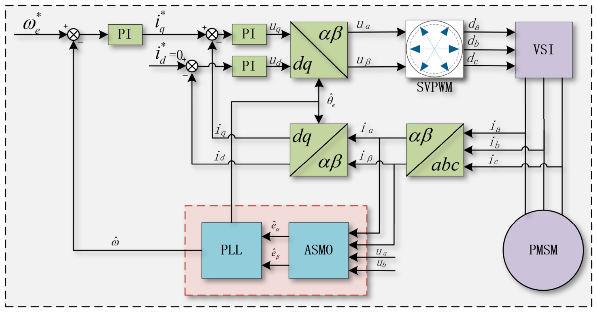
Figure 1. Structure of the sensorless PMSM FOC system.
Machines 14 01041 g001
Figure 2. Structure of the continuous-boundary-layer ASMO and second-order PLL.
Machines 14 01041 g002
Figure 3. Propagation path from VSI-nonlinearity-induced terminal-voltage mismatch to electrical-position error.
Machines 14 01041 g003
Figure 4. Structure of the proposed delay-aware VSI nonlinearity compensation method.
Machines 14 01041 g004
Figure 5. Experimental platform for PMSM sensorless control.
Machines 14 01041 g005
Figure 6. Results of the steady-state comparative evaluation for Schemes A, B, and E: (a) Scheme A without VSI nonlinearity compensation; (b) Scheme B with conventional compensation; and (c) Scheme E with the complete proposed compensation method.
Machines 14 01041 g006
Figure 7. (a) Existing delay-sensitivity and module-ablation simulation; (b) threshold selection analysis of I th ; and (c) robustness analysis with sampling noise and offset.
Machines 14 01041 g007
Figure 8. Temperature-parameterized simulation under a prescribed drift of the equivalent VSI distortion voltage: (a) externally scheduled temperature and prescribed amplitude drift; (b) fixed versus online amplitude tracking; (c) harmonic suppression across temperature; and (d) position-estimation robustness.
Machines 14 01041 g008
Figure 9. Factorial ablation results of prediction and cubic weighting modules: (a) compensation-voltage error comparison; (b) maximum compensation-voltage deviation; and (c) electrical-position error comparison.
Machines 14 01041 g009
Figure 10. Delay robustness under different switching frequencies and effective delay ratios: (a) polarity decision error; (b) compensation-voltage error; (c) position estimation error; and (d) improvement ratio of Scheme E.
Machines 14 01041 g010
Figure 11. Dynamic speed-tracking results with the conventional compensation scheme: (a) conventionally estimated and encoder-measured mechanical speeds; (b) conventionally estimated and encoder-measured electrical angles; (c) mechanical-speed difference; and (d) electrical-angle difference.
Machines 14 01041 g011
Figure 12. Dynamic speed-tracking results of the proposed scheme: (a) estimated and encoder mechanical speeds; (b) estimated and encoder electrical angles; (c) mechanical-speed difference; and (d) electrical-angle difference.
Machines 14 01041 g012
Figure 13. Common-condition load-disturbance comparison of Scheme B, Ref. [16], and Scheme E: (a) encoder-measured mechanical-speed response; (b) mechanical-speed estimation error; (c) electrical-position estimation error; and (d) maximum speed drop and recovery time. In panel (d), open circles show individual records, filled circles show means, and error bars indicate SD ( n = 3 ).
Machines 14 01041 g013
Figure 14. Common-condition current-quality comparison of Scheme B, Ref. [16], and Scheme E: (a) phase-current waveform; (b) phase-current FFT and THD 2 : 20 ; and (c) d-q-axis current response.
Machines 14 01041 g014
Figure 15. Online equivalent distortion-voltage amplitude update and electrical-position estimation error under different dead times: (a) estimated distortion-voltage amplitude, with the time axis including the 0.10 s initialization interval; (b) enabling state, with χ = 0 during INIT/HOLD and χ = 1 during TRACK; (c) electrical-position estimation error; and (d) steady-state error spectrum.
Machines 14 01041 g015
Figure 16. Hardware validation of automatic online-update freezing during q-axis current reversal: (a) speed response; (b) q-axis current reversal; (c) reversal-trigger pulse r rev , vertically offset for visibility, and the latched enabling state χ , with a local view; (d) estimated distortion-voltage amplitude and local HOLD-invariance view; and (e) electrical-position estimation error. The shaded interval denotes the automatically latched HOLD state.
Machines 14 01041 g016aMachines 14 01041 g016b
Table 1. Structural comparison with the closely related methods.
MethodDigital DelayActuation-Time PolarityContinuous Zero CrossingOnline AmplitudeCompensation Location
Ref. [4]NoNoNoYesCommand side
Ref. [15]NoNoNoYes, RLSCommand + observer inputs
Ref. [16]NoNoNoYes, RTLSCommand side
Ref. [24]No; discrete-time modelN/AN/AN/ASMO/PLL
Ref. [25]YesNo; current-value predictionN/AN/ACurrent-feedback/SMO path
Ref. [26]YesYes, reference-current signNo, hard signNo; adapts delay timePWM timing
Ref. [23]NoNoNoYes, MRASPWM duty ratio
This workYesYesYes, C 1 cubic weightYesReconstructed ASMO input
N/A indicates that the feature is not applicable because the cited method does not compensate VSI nonlinearity. Ref. [24] treats low-sampling-ratio discretization rather than sampling-to-actuation delay. Ref. [25] predicts actuation-time current values for delay precompensation but does not use their polarity to select a VSI-nonlinearity compensation direction. Ref. [26] adapts compensation time rather than distortion-voltage amplitude.
Table 2. Main parameters of the PMSM drive experimental platform and control system.
ItemSymbol or ConfigurationValue
Motor under testType/rated powerPMSM/200 W
Rated electrical parametersVoltage/current24 V/8 A
Tested mechanical-speed range n m 600–1500 r/min
Number of pole pairsp5
Stator resistance R s 0.128 Ω
d- and q-axis inductances L d / L q 0.153 mH
Permanent-magnet flux linkage ψ f 0.0166 Wb
Loading deviceType/torque capacityMagnetic powder brake/ 1 N · m
dc link V dc 24 V
ControllerMCU/clock frequencyLCM32F039/96 MHz
Sampling period T s 100 µs
Current-control period100 µs
PWM switching frequency f PWM 10 kHz
Dead time T dead 1 µs (baseline; 1–3 µs evaluated)
Effective sampling-to-actuation delay T d 100 µs
Current sensingADC resolution12 bit
Position ground truthMagnetic encoder resolution13 bit
Numerical implementationQ formatQ14
Zero-crossing threshold I th 0.2 A
Correlation-filter coefficient λ a 0.0609
Minimum excitation threshold q min 0.05
Back-EMF update-enable threshold3 V
Table 3. Metrics from the steady-state comparative evaluation of Schemes A, B, and E.
MetricScheme AScheme BScheme EImprovement of Scheme E over Scheme B
H 5 / H 1 (%)10.386.323.8139.72%
H 7 / H 1 (%)7.244.102.9029.27%
THD 2 : 20 ( e ^ α ) (%)24.2913.606.2154.33%
RMS of the electrical-position estimation error (°)3.612.141.1048.60%
Peak-to-peak electrical-position estimation error (°)10.867.824.7339.51%
Amplitude of the sixth-order electrical-position-error component (°)4.6302.7771.39649.73%
Table 4. Delay-sensitivity and module-ablation simulation results for Schemes B–E.
ComparisonSingle ModificationEvaluation MetricResult
B → CCurrently sampled current → predicted currentCurrent-polarity misclassification rate16.22% → 6.10%
C → DLinear zero-crossing weight → C1-continuous cubic zero-crossing weightMaximum compensation-voltage deviation0.339 V → 0.254 V
C → DLinear zero-crossing weight → C1-continuous cubic zero-crossing weightPeak-to-peak electrical-position error/sixth-order componentReduced by 13.4%/16.8%
D → EFixed equivalent distortion-voltage amplitude → online amplitude updateEquivalent distortion-voltage amplitude error/peak-to-peak electrical-position error0.116 V → 0.015 V; 4.21 3.44
E, 1.5 T s Delay mismatch and dual saturationMaximum compensation-voltage deviation≤1.941 V
Disclaimer/Publisher’s Note: The statements, opinions and data contained in all publications are solely those of the individual author(s) and contributor(s) and not of MDPI and/or the editor(s). MDPI and/or the editor(s) disclaim responsibility for any injury to people or property resulting from any ideas, methods, instructions or products referred to in the content.