Validation-Protected Physics-Consistent Probabilistic Neural Speed Estimation for Sensorless Permanent Magnet Synchronous Motor Drives

Abstract

Mechanical speed sensors increase cost and may reduce the reliability of permanent magnet synchronous motor (PMSM) drives under harsh conditions. This paper proposes a validation-protected physics-consistent probabilistic neural estimator for sensorless PMSM speed estimation using only online-deployable signals: the previous estimated speed, measured d/q-axis currents, and commanded d/q-axis voltages. A multi-output probabilistic network predicts the speed distribution and auxiliary residual-compensation variables. Mechanical consistency, electrical consistency, and regularization losses are imposed during training, while a validation-protected rule selects, for each random seed, the checkpoint with the lower validation RMSE from the paired baseline and physics-trained candidates. Experiments use a frozen multi-seed protocol covering locked holdout evaluation, independent comparison, and disturbance tests. Across Datasets 8–11, the frozen predictive distributions yielded Gaussian NLL values from 3.190 to 3.239, 100% empirical coverage of the nominal 95% prediction intervals, and mean interval widths of approximately 35.9 rad/s, indicating conservative rather than well-calibrated uncertainty. On locked Dataset 7, Physics-safe reduced the mean RMSE from 3.415 to 3.277 and the inter-seed standard deviation from 0.290 to 0.052. Results on Datasets 8–11 show that the method is not universally mean-error optimal; its recurring advantage is lower inter-seed variability and more reproducible training outcomes. A local sensitivity analysis on Dataset 4 confirmed seed- and loss-weight-dependent physics-training outcomes, supporting the need for validation protection without implying globally optimal loss weights. On the specified desktop CPU using ONNX Runtime, the complete recursive estimator step required 40.154 microseconds, below the adopted 100-microsecond sampling interval, supporting estimator-level computational feasibility.

1. Introduction

Permanent magnet synchronous motors (PMSMs) have been widely used in electric vehicles, industrial servo systems, robotics, and high-performance electromechanical drives because of their high power density, high efficiency, and fast dynamic response [1,2,3]. Accurate speed information is essential for field-oriented control, torque regulation, dynamic performance optimization, and fault-tolerant operation of PMSM drive systems. In conventional drive systems, mechanical position or speed sensors are commonly used to obtain rotor information. However, these sensors increase system cost, installation complexity, and maintenance burden, and their reliability may be degraded under harsh operating conditions such as high temperature, vibration, and electromagnetic interference [1,4,5,6]. Therefore, sensorless speed estimation remains an important topic for reliable and cost-effective PMSM drives [3].

In electrified transportation and DC power systems, motor drives operate within broader powertrain, energy-management, and power-conversion architectures. Recent studies have investigated degradation-aware energy management for plug-in fuel-cell hybrid vehicles and coordinated multi-loop control of current-source rectifiers in low-voltage DC distribution systems [7,8]. These studies address system-level energy allocation and converter control rather than the lower-level problem of sensorless PMSM speed estimation. Reliable rotor-speed estimation therefore remains a distinct enabling function for high-performance motor-drive control.

Existing sensorless estimation methods can be broadly divided into model-based observers and data-driven estimators. Model-based methods, such as extended Kalman filters, sliding-mode observers, model reference adaptive systems, and unscented Kalman filters, have clear physical interpretations and are attractive for engineering applications [1,4,5,9,10,11,12,13]. Nevertheless, their estimation accuracy usually depends on the correctness of motor parameters, noise assumptions, and model matching conditions. Variations in stator resistance, inductance, permanent magnet flux linkage, load torque, inverter nonidealities, and measurement noise may lead to biased estimation or degraded robustness [14,15,16,17,18]. These limitations become more evident when the drive operates over a wide speed range or under strong disturbance conditions.

In recent years, neural-network-based estimators have been increasingly investigated for motor state estimation, condition monitoring, and fault diagnosis [19,20,21,22]. Compared with purely model-based observers, neural networks can learn complex nonlinear mappings from measured data and can reduce the need for exact analytical modeling [19,20,21,22]. However, purely data-driven estimators also introduce new challenges. Their performance may be sensitive to random initialization, training data ordering, and optimization trajectories [23]. In addition, black-box neural estimators may generate predictions that are inconsistent with basic PMSM dynamics, especially under disturbance scenarios or operating conditions that differ from the training distribution [24,25,26,27,28]. As a result, a single training run or a single random seed may not be sufficient to characterize the reliability of a neural speed estimator [23,29,30]. Beyond point prediction, probabilistic neural-network methods provide mechanisms for representing predictive uncertainty, while prior work has emphasized the importance of distinguishing uncertainty sources, evaluating probabilistic forecasts with proper scoring rules, and explicitly assessing calibration and sharpness [31,32,33,34,35,36]. Physics-informed and physics-consistent learning provides a possible way to improve the robustness and interpretability of neural estimators by embedding physical constraints into the training objective [24,25,26,27,28]. For PMSM speed estimation, mechanical motion consistency and electrical dynamic consistency can be used to constrain the predicted speed and auxiliary variables associated with the physics-consistency constraints [24,25,26]. However, incorporating physical constraints does not necessarily guarantee improved estimation accuracy. Simplified motor equations may deviate from the real drive system because of parameter uncertainty, sampling effects, unmodeled disturbances, and inverter nonlinearities [14,15,16,17,18]. Moreover, multi-objective optimization with data and physics losses may cause training instability, and a physics-constrained checkpoint may even perform worse than a baseline neural checkpoint for some random seeds [23,29]. Therefore, a practical physics-consistent neural estimator should not only exploit physical knowledge but also avoid performance degradation caused by imperfect physical constraints.

Accordingly, this study tests the following hypothesis: validation-protected physics-consistent training can reduce random-seed sensitivity and narrow the distribution of seed-wise RMSE without requiring the physics-trained checkpoint to outperform the baseline checkpoint in mean RMSE under every operating condition. This hypothesis is evaluated using independently trained random seeds and a frozen dataset hierarchy that separates development and ablation, locked holdout evaluation, independent comparison, and supplementary disturbance testing.

To address these issues, this paper proposes a validation-protected physics-consistent probabilistic neural estimator for sensorless PMSM speed estimation. The estimator uses only online deployable signals, including the previous estimated speed, measured d/q-axis currents, and commanded d/q-axis voltages. A multi-output probabilistic neural network predicts the speed distribution parameters together with auxiliary residual-compensation variables. Mechanical consistency, electrical consistency, and regularization losses are incorporated during training to encourage predictions that remain compatible with basic PMSM dynamics.

In contrast to directly adopting a physics-trained checkpoint as the final estimator, the proposed framework treats physics-trained checkpoints as validation-screened candidate refinements. The baseline neural checkpoint is retained as a protected fallback whenever approximate physical constraints or multi-objective optimization degrade the validation RMSE. Therefore, the methodological contribution is not merely the addition of physical residuals to a neural loss function, but a validation-protected training and checkpoint-selection framework designed to improve inter-run reproducibility under imperfect physical models. In this work, the term “safe” refers specifically to protection against validation-performance degradation and does not denote formal control-theoretic safety certification.

The main contributions of this paper are summarized as follows:

• A probabilistic neural speed estimator is developed using only controller-available online signals. The network jointly predicts the speed distribution parameters and auxiliary residual-compensation variables, while the true speed, true load torque, and internal simulation disturbance variables are excluded from online inference.
• A validation-protected physics-consistent training framework is proposed. Physics-trained checkpoints are treated as candidate refinements rather than compulsory replacements, and the baseline checkpoint is retained whenever the physics-trained candidates produce a higher validation RMSE. This mechanism limits validation-performance degradation caused by approximate physical constraints and multi-objective optimization.
• A frozen evaluation hierarchy is established to separate method development from formal evaluation. Dataset 4 is used for development and ablation, Dataset 7 for locked holdout evaluation, Dataset 8 for independent comparison, and Datasets 9–11 for supplementary load disturbance, parameter mismatch, and noise disturbance evaluation. mismatch, and noise disturbance evaluation.
• The proposed estimator is evaluated using multiple independently trained random seeds. In addition to mean RMSE, the evaluation considers inter-seed RMSE variation, paired seed-wise comparisons, and error-distribution stability, thereby examining whether validation-protected physics consistency improves training reproducibility rather than universally minimizing mean estimation error.

The remainder of this paper is organized as follows: Section 2 introduces the PMSM model and formulates the sensorless speed estimation problem. Section 3 presents the proposed validation-protected physics-consistent probabilistic neural estimator. Section 4 describes the experimental setup and frozen evaluation protocol. Section 5 reports and discusses the experimental results. Finally, Section 6 concludes the paper and discusses future work.

2. PMSM Model and Problem Formulation

2.1. PMSM Model in the Synchronous Reference Frame

The electrical dynamics of a PMSM can be described in the synchronous rotating d/q reference frame [1,3,4]. By neglecting iron loss, magnetic saturation, and high-frequency parasitic effects, the stator voltage equations are given by

$$u_d=R_s{i}_d+L_d{\displaystyle \frac{d{i}_d}{dt}}-{\omega }_e{L}_q{i}_q,$$

(1)

$$u_q=R_s{i}_q+L_q{\displaystyle \frac{d{i}_q}{dt}}+{\omega }_e\left(L_d{i}_d+{\psi }_f\right),$$

(2)

where $u_d$ and $u_q$ are the d/q-axis stator voltages, $i_d$ and $i_q$ are the d/q-axis stator currents, $R_s$ is the stator resistance, $L_d$ and $L_q$ are the d/q-axis inductances, ${\psi }_f$ is the permanent magnet flux linkage, and ${\omega }_e$ is the electrical angular speed. The relationship between electrical angular speed and mechanical angular speed is

$${\omega }_e=p{\omega }_m,$$

(3)

where p is the number of pole pairs and ${\omega }_m$ is the mechanical angular speed.

The electromagnetic torque of the PMSM is expressed as

$$T_e={\displaystyle \frac{3}{2}}p\left[{\psi }_f{i}_q+\left(L_d-L_q\right)i_d{i}_q\right],$$

(4)

where $T_e$ denotes the electromagnetic torque. The mechanical motion equation is

$$J{\displaystyle \frac{d{\omega }_m}{dt}}=T_e-T_L-B{\omega }_m,$$

(5)

where J is the rotor inertia, B is the viscous friction coefficient, and $T_L$ is the load torque. Equations (1)–(5) describe the fundamental coupling among stator voltages, currents, electromagnetic torque, and rotor speed [24,25,26]. These relationships provide the physical basis for the consistency constraints introduced in the proposed neural estimator.

2.2. Sensorless Speed Estimation Problem

The objective of sensorless speed estimation is to estimate the mechanical angular speed without using a mechanical speed or position sensor [2,9,10,11]. In this work, the estimator is designed for recursive online inference. At discrete sampling instant k, the input vector is defined as

$${\mathbf{x}}_k={\left[{\widehat{\omega }}_m(k-1),i_d^{\mathrm{m}}(k-1),i_q^{\mathrm{m}}(k-1),u_{d,\mathrm{cmd}}\left(k\right),u_{q,\mathrm{cmd}}\left(k\right)\right]}^{\mathrm{T}},$$

(6)

where ${\widehat{\omega }}_m(k-1)$ is the previously estimated mechanical speed, $i_d^{\mathrm{m}}(k-1)$ and $i_q^{\mathrm{m}}(k-1)$ are the measured d/q-axis currents, and $u_{d,\mathrm{cmd}}\left(k\right)$ and $u_{q,\mathrm{cmd}}\left(k\right)$ are the commanded d/q-axis voltages.

The estimation target is the current mechanical speed,

$${\widehat{\omega }}_m\left(k\right)=f_{\theta }\left({\mathbf{x}}_k\right),$$

(7)

where $f_{\theta }(·)$ denotes the neural estimator with trainable parameters $\theta$.

This formulation reflects the recursive nature of sensorless speed estimation: the current prediction depends on the previous speed estimate and currently available electrical signals. It also avoids the use of non-deployable variables during online inference.

2.3. Online Deployability Constraint

For practical sensorless implementation, the proposed estimator is restricted to signals that can be obtained from the controller or measurement system during online operation. Specifically, the inference-stage input is limited to the previous estimated speed, measured d/q-axis currents, and commanded d/q-axis voltages, as defined in Equation (6).

The following variables are not used as external inputs during inference:

$${\omega }_m\left(k\right),T_L\left(k\right),T_e\left(k\right),d_{\mathrm{ext},k},\Delta u_{d,k},\Delta u_{q,k}.$$

(8)

Here, ${\omega }_m\left(k\right)$ is the reference mechanical speed, $T_L\left(k\right)$ is the true load torque, and $T_e\left(k\right)$ is the electromagnetic torque. The variables $d_{\mathrm{ext},k}$, $\Delta u_{d,k}$, and $\Delta u_{q,k}$ are internally predicted auxiliary residual-compensation variables. They participate only in the construction of the physics-consistency losses and are neither external online inputs nor directly supervised physical state estimates.

This deployability constraint is essential for a fair evaluation of sensorless estimation methods. If the true speed, true load torque, electromagnetic torque, or internal simulation variables were used as inference inputs, the resulting estimator could achieve artificially low errors but would not represent a practically deployable sensorless method. Therefore, all neural estimators and baseline methods considered in this work follow the same input constraint.

3. Proposed Method

3.1. Overall Framework

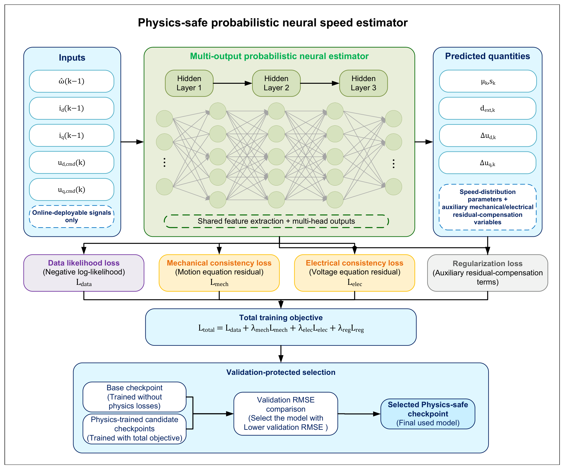
This section presents the proposed validation-protected physics-consistent probabilistic neural speed estimator, referred to as Physics-safe. The method consists of three main components: a baseline probabilistic neural estimator, physics-consistent training losses, and a validation-protected checkpoint selection mechanism. During online inference, the estimator uses only deployable signals, including the previous estimated speed, measured d/q-axis currents, and commanded d/q-axis voltages. During training, mechanical consistency and electrical consistency losses are introduced to constrain the estimator according to the PMSM dynamics described in Section 2.

In this paper, the term “safe” refers to validation-performance degradation protection. It does not indicate formal control-theoretic safety certification. The final model is selected from the baseline checkpoint and physics-trained candidate checkpoints according to validation RMSE, so that the estimator can avoid using a physics-trained checkpoint when physics-consistent training degrades validation performance.

Figure 1 illustrates the overall workflow of the proposed method, including the online-deployable inputs, multi-output probabilistic estimator, physics-consistency and regularization losses, and validation-protected checkpoint selection. The auxiliary mechanical and electrical outputs shown in the figure are residual-compensation variables used in the physics-consistency training objective rather than directly supervised physical estimates.

3.2. Input–Output Design and Probabilistic Neural Estimator

According to the online deployability constraint defined in Section 2, the estimator uses only the input vector ${\mathbf{x}}_k$, which contains the previous estimated speed, measured d/q-axis currents, and commanded d/q-axis voltages. The multi-output neural estimator is formulated as

$${\mathbf{y}}_k=f_{\theta }\left({\mathbf{x}}_k\right),$$

(9)

where

$${\mathbf{y}}_k=[{\mathsf{\mu }}_k,s_k,d_{\mathrm{ext},k},\Delta u_{d,k},\Delta u_{q,k}{]}^{\mathrm{T}}.$$

(10)

Here, ${\mathsf{\mu }}_k$ is the predicted speed mean, $s_k$ is the predicted log-variance, $d_{\mathrm{ext},k}$ is an auxiliary mechanical residual-compensation variable, and $\Delta u_{d,k}$ and $\Delta u_{q,k}$ are auxiliary electrical residual-compensation variables. These auxiliary outputs enter the physics-consistency residuals and are regularized during training, but they are not directly supervised as load-torque or inverter-voltage-error estimates and are not assumed to be uniquely physically identifiable. In the implementation, the speed target is normalized by a fixed scale of $500\mathrm{rad}/\mathrm{s}$, the mean and log-variance heads operate in the normalized coordinates, and the output is transformed back to physical units for recursive inference and evaluation. For numerical stability, the implemented log-variance output is clipped to $[-8,6]$. The estimated mechanical speed remains defined by Equation (11).

The estimated mechanical speed is

$${\widehat{\omega }}_m\left(k\right)={\mathsf{\mu }}_k.$$

(11)

The probabilistic output is used to construct a Gaussian negative log-likelihood loss. Over a rolling training window of length H, the data likelihood loss is defined as

$${\mathcal{L}}_{\mathrm{data}}={\displaystyle \frac{1}{H}}{\displaystyle \sum _{k=1}^H}\left[{\displaystyle \frac{{\left({\omega }_m\left(k\right)-{\mathsf{\mu }}_k\right)}^2}{2\exp \left(s_k\right)}}+{\displaystyle \frac{1}{2}}{s}_k\right],$$

(12)

where ${\omega }_m\left(k\right)$ is the reference speed. The log-variance output $s_k$ allows the network to model heteroscedastic prediction uncertainty during training.

3.3. Mechanical Consistency Constraint

The mechanical consistency constraint is constructed from the electromagnetic torque equation and the mechanical motion equation of the PMSM. Based on the measured currents, the electromagnetic torque-related quantity is computed as

$${\widehat{T}}_{e,k}={\displaystyle \frac{3}{2}}p\left[{\psi }_f{i}_{q,k-1}^{\mathrm{m}}+\left(L_d-L_q\right)i_{d,k-1}^{\mathrm{m}}{i}_{q,k-1}^{\mathrm{m}}\right],$$

(13)

where p is the number of pole pairs, ${\psi }_f$ is the permanent magnet flux linkage, and $L_d$ and $L_q$ are the d/q-axis inductances.

Using a forward Euler approximation of the mechanical motion equation, the mechanical residual is defined as

$$r_{\mathrm{mech},k}=J{\displaystyle \frac{{\mathsf{\mu }}_k-{\omega }_{k-1}^{\mathrm{in}}}{T_s}}-\left({\widehat{T}}_{e,k}-d_{\mathrm{ext},k}-B{\mathsf{\mu }}_k\right),$$

(14)

where J is the rotor inertia, B is the viscous friction coefficient, $T_s$ is the sampling period, and ${\omega }_{k-1}^{\mathrm{in}}$ denotes the speed input used by the recursive estimator at the previous step. The mechanical consistency loss is

$${\mathcal{L}}_{\mathrm{mech}}={\displaystyle \frac{1}{H}}{\displaystyle \sum _{k=1}^H}{r}_{\mathrm{mech},k}^2.$$

(15)

The auxiliary mechanical residual-compensation variable $d_{\mathrm{ext},k}$ is predicted internally by the neural network. It is not used as an external inference input and is introduced only to support the mechanical consistency residual during training; it is not directly supervised as a load-torque estimate.

3.4. Electrical Consistency Constraint

The electrical consistency constraint is used to regularize the auxiliary electrical residual-compensation variables according to the d/q-axis current dynamics. The effective d/q-axis voltages are defined as

$${\overline{u}}_{d,k}=u_d^{*}\left(k\right)+\Delta u_{d,k},$$

(16)

$${\overline{u}}_{q,k}=u_q^{*}\left(k\right)+\Delta u_{q,k},$$

(17)

where $u_d^{*}\left(k\right)$ and $u_q^{*}\left(k\right)$ are the commanded d/q-axis voltages. The predicted electrical angular speed is

$${\widehat{\omega }}_{e,k}=p{\mathsf{\mu }}_k.$$

(18)

According to the discretized d/q-axis electrical dynamics, the one-step current predictions are given by

$${\widehat{i}}_{d,k}=i_{d,k-1}^{\mathrm{m}}+{\displaystyle \frac{T_s}{L_d}}\left[{\overline{u}}_{d,k}-R_s{i}_{d,k-1}^{\mathrm{m}}+{\widehat{\omega }}_{e,k}{L}_q{i}_{q,k-1}^{\mathrm{m}}\right],$$

(19)

$${\widehat{i}}_{q,k}=i_{q,k-1}^{\mathrm{m}}+{\displaystyle \frac{T_s}{L_q}}\left[{\overline{u}}_{q,k}-R_s{i}_{q,k-1}^{\mathrm{m}}-{\widehat{\omega }}_{e,k}\left(L_d{i}_{d,k-1}^{\mathrm{m}}+{\psi }_f\right)\right].$$

(20)

The electrical consistency loss is defined as

$${\mathcal{L}}_{\mathrm{elec}}={\displaystyle \frac{1}{H}}{\displaystyle \sum _{k=1}^H}g\left({\omega }_{k-1}^{\mathrm{in}}\right)\left[{\left({\widehat{i}}_{d,k}-i_{d,k}^{\mathrm{m}}\right)}^2+{\left({\widehat{i}}_{q,k}-i_{q,k}^{\mathrm{m}}\right)}^2\right],$$

(21)

where $i_{d,k}^{\mathrm{m}}$ and $i_{q,k}^{\mathrm{m}}$ are the measured d/q-axis currents, H is the rolling training window length, and $g(·)$ is a speed-dependent gating function. This loss encourages the predicted currents to remain consistent with the measured currents while allowing the electrical consistency constraint to be weighted according to the speed-dependent operating condition.

In the present implementation, the speed-dependent gating function is defined as

$$g\left({\omega }_{k-1}^{\mathrm{in}}\right)={\displaystyle \frac{\left|{\omega }_{k-1}^{\mathrm{in}}\right|}{\left|{\omega }_{k-1}^{\mathrm{in}}\right|+{\omega }_{\mathrm{c}}+ϵ}},$$

where ${\omega }_{\mathrm{c}}=50\times 2\pi /60\mathrm{rad}/\mathrm{s}\approx 5.236\mathrm{rad}/\mathrm{s}$ and $ϵ={10}^{-8}$. The value of 50 r/min was adopted as a fixed engineering low-speed boundary to attenuate the electrical residual in the region where back-EMF-related observability is weak. It was not obtained through an exhaustive search on Dataset 4 and is not derived from a specific rated motor parameter or hardware component. Therefore, it should not be interpreted as a universally optimal threshold. The gating function smoothly restores the electrical-consistency contribution as the speed increases.

3.5. Regularization and Total Training Objective

The auxiliary residual-compensation variables $d_{\mathrm{ext},k}$, $\Delta u_{d,k}$, and $\Delta u_{q,k}$ improve the flexibility of the physics-consistency residuals. However, if they are not constrained, the network may overuse these variables and weaken the intended role of the consistency losses. Therefore, the following regularization loss is introduced:

$${\mathcal{L}}_{\mathrm{reg}}={\displaystyle \frac{1}{H}}{\displaystyle \sum _{k=1}^H}\left[d_{\mathrm{ext},k}^2+\Delta u_{d,k}^2+\Delta u_{q,k}^2\right].$$

(22)

Combining the data likelihood loss, mechanical consistency loss, electrical consistency loss, and regularization loss, the total training objective is defined as

$${\mathcal{L}}_{\mathrm{total}}={\mathcal{L}}_{\mathrm{data}}+{\lambda }_{\mathrm{mech}}{\mathcal{L}}_{\mathrm{mech}}+{\lambda }_{\mathrm{elec}}{\mathcal{L}}_{\mathrm{elec}}+{\lambda }_{\mathrm{reg}}{\mathcal{L}}_{\mathrm{reg}}.$$

(23)

Here, ${\lambda }_{\mathrm{mech}}$, ${\lambda }_{\mathrm{elec}}$, and ${\lambda }_{\mathrm{reg}}$ are non-negative loss weighting coefficients.

The reference setting used in the frozen formal evaluations was ${\lambda }_{\mathrm{mech}}={10}^{-4}$, ${\lambda }_{\mathrm{elec}}={10}^{-4}$, and ${\lambda }_{\mathrm{reg}}={10}^{-6}$. These coefficients were fixed during the original method-development stage as an order-of-magnitude reference configuration rather than being selected through an exhaustive grid search. To quantify the local dependence on this choice, a one-factor-at-a-time sensitivity analysis was subsequently conducted on Dataset 4. Each coefficient was independently varied by one order of magnitude while the other two coefficients were held fixed. This supplementary analysis was used only for development-stage characterization and did not alter the frozen loss weights, checkpoint-selection rule, or models evaluated on Datasets 7–11.

During rolling prediction training, the speed predicted at the previous step is used as part of the input for the next step. This strategy reduces the distribution mismatch between training and recursive online inference.

3.6. Validation-Protected Checkpoint Selection

Physics-consistent training may improve validation performance for some random seeds, but it may also degrade validation performance when the simplified physical model is imperfect or when multi-loss optimization becomes unstable. To reduce this risk, the proposed method uses a validation-protected checkpoint selection mechanism.

For each random training seed, a baseline model is first trained using only the data likelihood loss in Equation (12). The resulting baseline checkpoint is denoted by ${\theta }_{\mathrm{base}}$. Starting from this baseline checkpoint, physics-consistent training is then performed using the total loss in Equation (23). This process produces a set of physics-trained candidate checkpoints:

$${\mathrm{\Theta }}_{\mathrm{phys}}={\theta }_{\mathrm{phys}}^{\left(1\right)},{\theta }_{\mathrm{phys}}^{\left(2\right)},\dots ,{\theta }_{\mathrm{phys}}^{\left(M\right)},$$

(24)

where M denotes the number of saved candidate checkpoints during physics-consistent training.

The final Physics-safe checkpoint is selected according to validation RMSE:

$${\theta }_{\mathrm{safe}}=\arg \underset{\theta \in {\theta }_{\mathrm{base}}\cup {\mathrm{\Theta }}_{\mathrm{phys}}}{\min }{\mathrm{RMSE}}_{\mathrm{val}}\left(\theta \right).$$

(25)

Therefore, when physics-consistent training improves validation performance, a physics-trained checkpoint is selected. When physics-consistent training causes validation degradation, the method can fall back to the baseline checkpoint. This mechanism changes physics-consistent training from a compulsory replacement strategy into a validation-protected candidate refinement strategy.

3.7. Method Boundary and Deployability

The proposed Physics-safe estimator follows the online deployability constraint defined in Section 2. During inference, it does not use the true speed, true load torque, true electromagnetic torque, or internal simulation disturbance variables. The auxiliary residual-compensation variables are predicted internally by the neural network and are used in the physics-consistency residuals and regularization term during training. They are not external inference inputs and are not directly supervised as estimates of the true load torque or physical inverter-voltage errors.

The proposed method is not intended to guarantee the lowest mean RMSE under all operating conditions. Its main objective is to reduce random seed sensitivity, improve training stability, and obtain more stable error distributions under disturbance scenarios. Therefore, Physics-safe should be interpreted as a validation-protected and stability-enhanced neural speed estimation method rather than a universally mean-error-optimal estimator. The proposed method is primarily intended for repeated offline training or batch model-generation settings in which reproducibility across independent training runs is important. It is not designed to guarantee the lowest estimation error for a single retrospectively selected training run. Accordingly, its intended role is to reduce seed-dependent deployment variation rather than to replace methods optimized solely for best-case single-model accuracy. No production-line calibration claim is made because no production-line, hardware-in-the-loop, or physical motor-drive experiment was conducted.

The present estimator predicts mechanical speed and does not independently reconstruct rotor electrical position. The current implementation assumes that the measured d/q -axis currents and commanded d/q-axis voltages have been formed by the surrounding controller-side synchronous-reference-frame transformation. Therefore, the proposed network should be interpreted as a speed-estimation module within a broader drive-control architecture rather than as a complete stand-alone position-and-speed observer. Reference-frame-angle errors may propagate into the transformed d/q quantities and may consequently degrade speed estimation. This coupling was not independently quantified under the present simulation protocol.

4. Experimental Setup and Evaluation Protocol

4.1. Experimental Objective

The experimental objective of this work is not only to compare the lowest mean estimation error on a single test set, but also to evaluate the stability and robustness of neural speed estimators under multiple random seeds and disturbance scenarios. The proposed Physics-safe estimator is therefore assessed from three perspectives: mean estimation accuracy, sensitivity to random training seeds, and robustness under additional disturbance conditions.

To avoid overinterpreting a single training run, all neural-network-based methods are evaluated using multiple independently trained checkpoints. The mean RMSE is used to measure the overall estimation accuracy, while the inter-seed standard deviation of RMSE is used to quantify the sensitivity of the estimator to random initialization and training stochasticity.

4.2. Simulation Model and Reference PMSM Parameters

All datasets were generated using the same PMSM drive simulation structure. The reference electrical and mechanical parameters used in the physics-consistency calculations and frozen disturbance protocols are summarized in

Table 1. Reference PMSM parameters and simulation configuration.

Parameter	Symbol	Value
Stator resistance	$R_s$	$0.1375\mathsf{\Omega }$
d-axis inductance	$L_d$	$7.76\times {10}^{-4}\mathrm{H}$
q-axis inductance	$L_q$	$7.76\times {10}^{-4}\mathrm{H}$
Permanent-magnet flux linkage	${\psi }_f$	$0.094945\mathrm{Wb}$
Rotor inertia	J	$0.00774\mathrm{kg}{\mathrm{m}}^2$
Viscous friction coefficient	B	$0.0016\mathrm{N}\mathrm{m}\mathrm{s}/\mathrm{rad}$
Number of pole pairs	p	4
Simulation duration	$T_{\mathrm{sim}}$	$10\mathrm{s}$
Export sampling period	$T_s$	$1\times {10}^{-4}\mathrm{s}$

. The simulation interval was 0–$10\mathrm{s}$, and the exported signals were uniformly sampled at $T_s=1\times {10}^{-4}\mathrm{s}$. These values define the nominal parameter set used as the reference configuration. Dataset-specific changes in speed excitation, load torque, parameter mismatch, and input-channel disturbance are described separately in Section 4.3. In particular, Dataset 10 applies predefined parameter mismatch relative to the nominal parameter set.

For all neural-network-based experiments, the sampling period was set to $T_s=1\times {10}^{-4}\mathrm{s}$, and the rolling training-window length was $H=6$. The Physics-safe estimator used a multi-output fully connected neural network with three hidden layers, 128 neurons in each hidden layer, and Tanh activation. The Adam optimizer was used with a learning rate of $5\times {10}^{-6}$, a batch size of 64, a maximum of 20 training epochs, and a weight decay of $1\times {10}^{-6}$. The frozen reference loss weights were ${\lambda }_{\mathrm{mech}}={10}^{-4}$, ${\lambda }_{\mathrm{elec}}={10}^{-4}$, and ${\lambda }_{\mathrm{reg}}={10}^{-6}$.

4.3. Dataset Usage Protocol and Evidence Roles

A hierarchical dataset usage protocol is adopted to reduce information leakage between method development and formal testing. Dataset 4 is used for method development, validation selection, component ablation analysis, and local loss-weight sensitivity analysis. It provides development evidence and mechanism explanation, but it is not used as the main evidence for formal generalization claims. The corresponding dataset roles and evidence hierarchy are summarized in

Table 2. Dataset usage and evidence hierarchy.

Dataset	Usage	Evidence Role
Dataset 4	Development, ablation, and loss-weight sensitivity	Development evidence
Dataset 7	Locked holdout evaluation	Method-freezing evidence
Dataset 8	Independent strong comparison	Main formal test evidence
Dataset 9	Load disturbance test	Supplementary robustness evidence
Dataset 10	Parameter mismatch test	Supplementary robustness evidence
Dataset 11	Noise disturbance test	Supplementary robustness evidence

.

For development-stage configuration screening, component ablation, and local loss-weight sensitivity analysis, Dataset 4 was divided into a 20,000-sample tuning subset and a disjoint 20,000-sample validation subset. The tuning subset was used for physics-consistent training under the candidate configurations, whereas the validation subset was used for checkpoint selection and development-stage reporting. Neither subset was treated as formal locked-test evidence, and no dataset from the locked formal evaluation hierarchy was accessed during the sensitivity study.

For the independently generated formal and supplementary test sets, Datasets 8–11 were simulated over 0–$10\mathrm{s}$. A common locked scoring interval of $[7.05,9.05)\mathrm{s}$ was extracted at $T_s=1\times {10}^{-4}\mathrm{s}$, yielding 20,000 samples in each locked window. The first sample was used only to initialize the recursive estimator and was excluded from scoring, leaving 19,999 scored samples per dataset and checkpoint. The speed-reference profiles combine two sinusoidal components with smooth rise and drop transitions. The specific load, parameter, and measurement-channel conditions are summarized in

Table 3. Generation and evaluation conditions for the independent locked test datasets.

Dataset	Scoring Window	Window Samples	Test Condition
8	$[7.05,9.05)$ s	20,000	$T_L:2.05\to 5.25\mathrm{N}\mathrm{m}$ at $8.08\mathrm{s}$
9	$[7.05,9.05)$ s	20,000	$T_L:2.05\to 5.25\mathrm{N}\mathrm{m}$ at $7.60\mathrm{s}$
10	$[7.05,9.05)$ s	20,000	$T_L:2.05\to 4.85\mathrm{N}\mathrm{m}$ at $7.70\mathrm{s}$; parameter mismatch
11	$[7.05,9.05)$ s	20,000	$T_L:2.05\to 4.85\mathrm{N}\mathrm{m}$ at $7.70\mathrm{s}$; input noise and ripple

. These datasets were generated only after the relevant model configurations had been frozen and were not used for training, hyperparameter tuning, architecture selection, or checkpoint selection.

For Dataset 10, the plant parameters were changed to $1.15R_s$, $0.90L_d$, $0.90L_q$, $0.92{\psi }_f$, $1.20J$, and $1.20B$, while all evaluated models retained their previously frozen checkpoints and settings. For Dataset 11, the plant parameters remained at the reference values. The noise realization was fixed using pseudorandom seed 1102026. Independent zero-mean Gaussian noise with a standard deviation of $0.035\mathrm{A}$ was added to both measured-current channels, whereas independent zero-mean Gaussian noise with a standard deviation of $0.025\mathrm{V}$ was added to both commanded-voltage channels. Deterministic sinusoidal voltage ripple with an amplitude of $0.035\mathrm{V}$ was additionally applied at $37\mathrm{Hz}$ and $43\mathrm{Hz}$ to the d- and q-axis commanded-voltage channels, respectively. The true speed and privileged physical variables were not corrupted and were used only for offline metric computation.

Dataset 7 is used for locked holdout evaluation and for determining the final reported method. After the evaluation on Dataset 7, no further modification is made to the model structure, loss weights, training seeds, or checkpoint selection rule.

After the final method and checkpoints are frozen, Dataset 8 is used as the main independent comparison dataset. Dataset 9, Dataset 10, and Dataset 11 are used to evaluate the frozen models under load disturbance, parameter mismatch, and noise disturbance scenarios, respectively. These additional disturbance test datasets are not used for training, hyperparameter tuning, or model selection.

4.4. Compared Methods

The following methods are compared in this work. Base denotes the baseline probabilistic neural speed estimator trained only with the data fitting loss. Physics-safe denotes the proposed validation-protected physics-consistent probabilistic neural speed estimator. LSTM and GRU are used as recurrent neural-network baselines [37,38]. In addition, UKF-based observers are used as conventional model-based reference methods in the independent comparison.

All neural-network-based methods use the same type of deployable inference inputs, including measured currents, commanded voltages, and the previous estimated speed. The true speed, true load torque, true electromagnetic torque, and internal simulation disturbance variables are not used as inference inputs.

4.5. Multiple Random Seeds and Model Freezing

Because neural network training is affected by random initialization, mini-batch ordering, and optimization trajectories, a single training seed may not reliably represent the performance of a method. Therefore, Base, Physics-safe, GRU, and LSTM are each evaluated with 12 frozen training seeds. Each seed corresponds to an independently trained checkpoint.

For the proposed Physics-safe method, each seed first produces a Base checkpoint. Physics-consistent training is then performed from the corresponding Base checkpoint, and the validation-protected selection rule is used to determine the final checkpoint for that seed. During the formal test stage, all checkpoints are fixed and read-only. No model retraining, hyperparameter adjustment, or checkpoint reselection is allowed according to the test results.

4.6. Loss-Weight Sensitivity Protocol

A local one-factor-at-a-time sensitivity analysis was conducted to evaluate the dependence of physics-consistent training on the three loss weights. The reference configuration was $({\lambda }_{\mathrm{mech}},{\lambda }_{\mathrm{elec}},{\lambda }_{\mathrm{reg}})=({10}^{-4},{10}^{-4},{10}^{-6})$. Six perturbed configurations were constructed by independently decreasing or increasing one coefficient by one order of magnitude while retaining the other two coefficients at their reference values. Together with the reference configuration, seven configurations were evaluated.

Each configuration was evaluated using the three predefined training seeds 11, 22, and 33, resulting in 21 training runs. Each run was initialized from the corresponding seed-specific Base checkpoint. Physics-consistent training was performed using the Dataset 4 tuning subset, and the Base and physics-trained candidate checkpoints were compared using the disjoint Dataset 4 validation subset. The protected checkpoint for each run was defined as the checkpoint with the lower validation RMSE. No locked or independent test dataset was accessed during this analysis.

4.7. Evaluation Metrics and Statistical Analysis

The root mean square error, abbreviated as RMSE, is used as the primary speed estimation error metric:

$$\mathrm{RMSE}=\sqrt{{\displaystyle \frac{1}{N}}\sum _{k=1}^N{\left({\widehat{\omega }}_m\left(k\right)-{\omega }_m\left(k\right)\right)}^2},$$

(26)

where N is the number of test samples, ${\widehat{\omega }}_m\left(k\right)$ is the estimated mechanical speed, and ${\omega }_m\left(k\right)$ is the reference mechanical speed. RMSE reflects the overall estimation error and is more sensitive to large deviations, so it is used as the primary metric in this work.

To evaluate the probabilistic output in addition to the point-estimation error, Gaussian negative log-likelihood (NLL), empirical 95% prediction interval coverage probability (PICP), and mean prediction interval width (MPIW) are additionally reported for the frozen Physics-safe estimator.

The equations in Section 3 use physical-speed notation. In the implementation, however, the network mean and log-variance outputs are represented in normalized speed coordinates. Let ${\mathsf{\mu }}_k^{\mathrm{norm}}$ and $s_k^{\mathrm{norm}}$ denote these normalized outputs. They are restored to physical units using the fixed speed scale $c_{\omega }=500\mathrm{rad}/\mathrm{s}$:

$${\mathsf{\mu }}_k^{\omega }=c_{\omega }{\mathsf{\mu }}_k^{\mathrm{norm}},{\sigma }_k^{\omega }=c_{\omega }\exp \left({\displaystyle \frac{s_k^{\mathrm{norm}}}{2}}\right),$$

(27)

where ${\mathsf{\mu }}_k^{\omega }$ and ${\sigma }_k^{\omega }$ are the predictive mean and standard deviation in $\mathrm{rad}/\mathrm{s}$, respectively.

The evaluation NLL includes the Gaussian normalization constant and is calculated as

$$\mathrm{NLL}={\displaystyle \frac{1}{N}}{\displaystyle \sum _{k=1}^N}\left[{\displaystyle \frac{1}{2}}\log \left(2\pi {\left({\sigma }_k^{\omega }\right)}^2\right)+{\displaystyle \frac{{\left({\omega }_m\left(k\right)-{\mathsf{\mu }}_k^{\omega }\right)}^2}{2{\left({\sigma }_k^{\omega }\right)}^2}}\right].$$

(28)

The empirical coverage probability of the nominal 95% prediction interval is defined as

$${\mathrm{PICP}}_{95}={\displaystyle \frac{1}{N}}{\displaystyle \sum _{k=1}^N}\mathbf{1}\left\{\left|{\omega }_m\left(k\right)-{\mathsf{\mu }}_k^{\omega }\right|\le 1.96{\sigma }_k^{\omega }\right\},$$

(29)

where $\mathbf{1}\{·\}$ is the indicator function. The corresponding mean prediction interval width is

$${\mathrm{MPIW}}_{95}={\displaystyle \frac{1}{N}}{\displaystyle \sum _{k=1}^N}2\left(1.96\right){\sigma }_k^{\omega }.$$

(30)

These probabilistic metrics are evaluated on Datasets 8–11 using the same 12 frozen Physics-safe checkpoints and the same locked scoring windows as the point-estimation analysis. The first sample is used only to initialize the recursive estimator and is excluded, leaving 19,999 evaluated samples per dataset and checkpoint. No model retraining, fine-tuning, variance rescaling, post hoc calibration, hyperparameter adjustment, or checkpoint reselection is performed for this diagnostic evaluation.

Because neural-network-based estimators are affected by random initialization, mini-batch ordering, and stochastic optimization, a single training seed may not reliably represent the performance of a method. This issue is especially important for PMSM speed estimation under wide-speed-range and disturbance conditions, where different random seeds may lead to different local optima and visible performance variation.

Therefore, for each neural-network-based method, the RMSE values obtained from 12 independently trained random seeds are reported. The mean, sample standard deviation, median, minimum, and maximum RMSE values are calculated. The mean RMSE is used to evaluate average estimation accuracy, while the inter-seed RMSE standard deviation is used to evaluate the sensitivity of the method to random initialization and training stochasticity.

Paired win–tie–loss comparisons are also used to compare two methods under the same random seeds. In addition, a two-sided sign test is conducted. When the p-value is less than 0.05, the paired comparison is regarded as statistically significant. When the p-value is not less than 0.05, the result is described only as a numerical trend or stability difference, rather than as a statistically significant superiority claim.

4.8. Evaluation Boundary

All formal evaluations in this work are limited to the current PMSM simulation model, data generation protocol, and frozen model set. The results can demonstrate the estimation stability and disturbance robustness of the proposed method under the present simulation conditions, but they should not be directly interpreted as final performance conclusions for an experimental test bench or hardware-in-the-loop platform.

In addition, the term “safe” in Physics-safe denotes validation-performance degradation protection. It does not indicate formal safety certification in the control-theoretic sense. Therefore, the following result analysis avoids claiming that Physics-safe is the mean-RMSE-optimal method under all operating conditions. Instead, the discussion focuses on its stability advantage under multiple random seeds and disturbance scenarios.

Overshoot and regulation time are closed-loop drive-control metrics jointly determined by the speed controller, current controller, inverter, motor plant, and estimator. The present study evaluates the recursive speed-estimation module under a frozen simulation protocol and therefore does not attribute closed-loop overshoot or settling time solely to the estimator. The current test profiles include smooth speed transitions and load changes, but they do not constitute dedicated physical speed-step, start-up, reversal, or low-speed steady-state experiments. Closed-loop evaluation of overshoot, settling time, steady-state bias, and low-speed fluctuation remains a subject for hardware-in-the-loop and motor-test-bench validation.

4.9. Inference-Time Benchmark Protocol

To evaluate the computational feasibility of the proposed estimator relative to the sampling period, an inference-time benchmark was conducted after the model architecture, parameters, and checkpoint-selection rule had been frozen. No dataset was accessed, and no training, hyperparameter tuning, or checkpoint reselection was performed during this benchmark.

The frozen Physics-safe checkpoint corresponding to seed 22 was used as the representative checkpoint. The network architecture and tensor dimensions are identical across the evaluated random seeds; therefore, the execution-time measurement characterizes the computational graph rather than the estimation accuracy of a particular seed. The checkpoint was exported to the ONNX format and executed using ONNX Runtime with the CPU execution provider. Both the intra-operation and inter-operation thread counts were fixed to one to reduce variability caused by multithreaded scheduling.

The benchmark was performed on an Intel Core i5-10200H processor under 64-bit Windows 11. For each timing scope, 5000 warm-up steps were executed before measurement. Subsequently, 20 independent repetitions were conducted, with 20,000 timed estimator steps in each repetition. Two timing scopes were evaluated. The first scope measured the preallocated ONNX Runtime session call. The second scope measured the complete recursive estimator step, including input-buffer updating, ONNX inference, output retrieval, and feedback of the estimated speed to the input of the next sampling instant. The reference sampling period was $T_s=1\times {10}^{-4}\mathrm{s}=100\mathsf{\mu }\mathrm{s}$.

5. Results and Discussion

5.1. Development Validation and Ablation Study

The first experiment investigates the contribution of the main training components in the proposed Physics-safe estimator. This experiment is conducted on Dataset 4, which is used only for method development, validation selection, and mechanism interpretation. Therefore, the results in this subsection are used to explain the role of each component rather than to support formal generalization claims.

Table 4. Ablation results on Dataset 4.

Method	Mean RMSE	Standard Deviation
Base	0.523311	0.211066
Physics-safe	0.250073	0.210975
Without mechanical consistency	3.147628	0.415988
Without electrical consistency	12.630956	2.073778
Without regularization	12.007696	0.936524

and Figure 2 present the ablation results on Dataset 4.

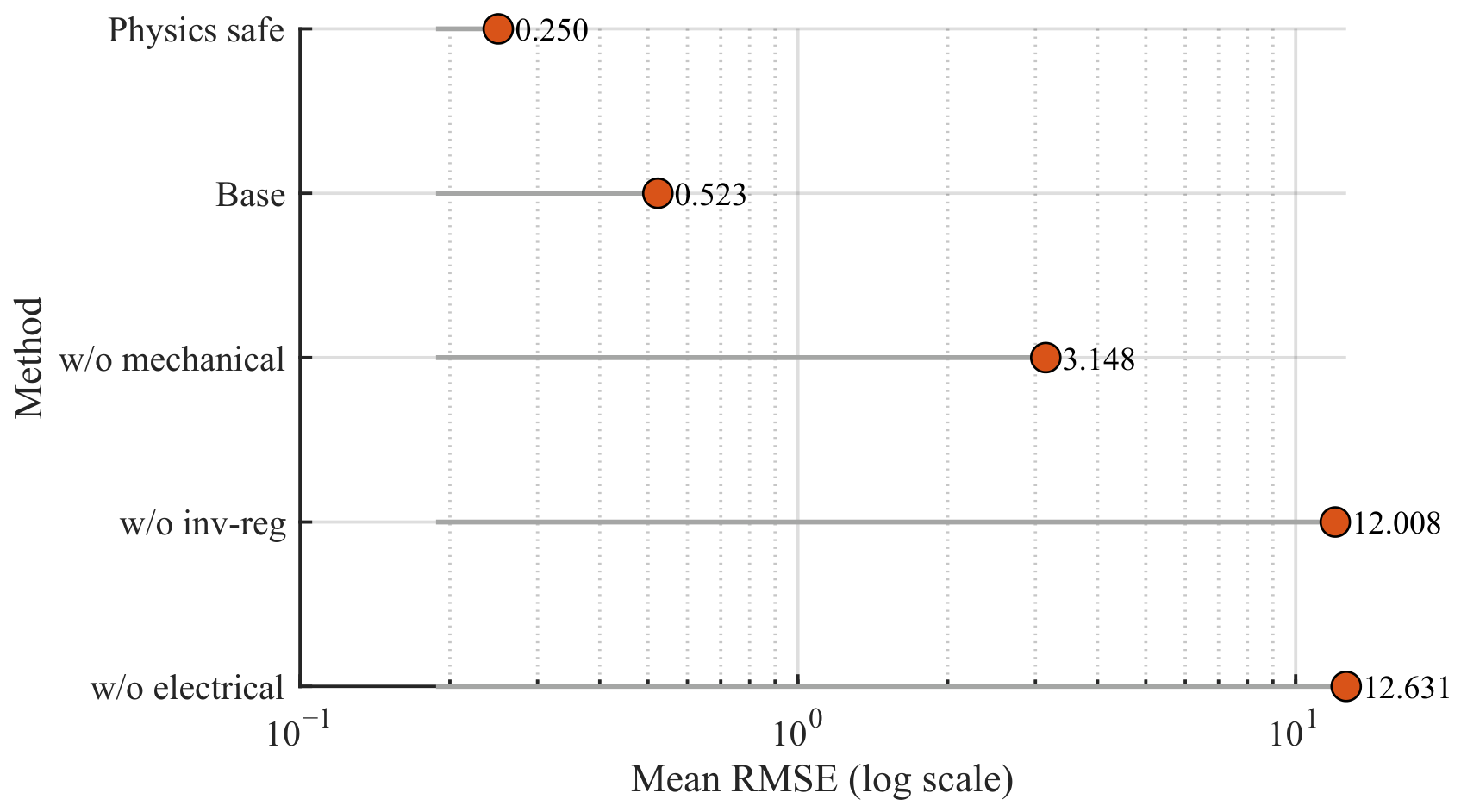
As shown in Table 4 and Figure 2, the complete Physics-safe configuration achieves a lower mean RMSE than the Base model on Dataset 4. Removing the mechanical consistency loss, electrical consistency loss, or regularization term leads to a substantial increase in estimation error, indicating that these components are not merely auxiliary additions but play important roles in constraining the neural estimator and its auxiliary residual-compensation variables.

Among the three removed components, the removal of the electrical consistency loss causes the largest error increase. This suggests that the d/q-axis electrical dynamic constraint provides a strong and useful physical restriction for the present PMSM speed estimation task. The regularization term is also necessary, because without it the auxiliary residual-compensation variables may be overused and may weaken the intended role of the physics-consistency constraints.

It should be emphasized that Dataset 4 is used for development validation and component-level interpretation. The results in this subsection show that the proposed physical consistency terms are useful during method development, but they are not used as the primary evidence for formal generalization performance.

A separate local sensitivity analysis is reported in the following subsection to examine whether the development-stage behavior depends excessively on the selected loss weights. This analysis also uses only the Dataset 4 tuning and validation subsets and does not modify the frozen configuration used in the subsequent formal evaluations.

5.2. Loss-Weight Sensitivity Analysis

Table 5. Local loss-weight sensitivity results on the Dataset 4 validation subset over three predefined seeds. RMSE values are reported as mean ± sample standard deviation. P/B denotes the numbers of physics-trained and Base checkpoints selected, respectively.

Configuration	Weight Triplet	Physics-Trained RMSE	Protected RMSE	Selected P/B
M-low	$({10}^{-5},{10}^{-4},{10}^{-6})$	$1.843\pm 0.404$	$0.535\pm 0.269$	0/3
Reference	$({10}^{-4},{10}^{-4},{10}^{-6})$	$1.009\pm 1.420$	$0.368\pm 0.309$	2/1
M-high	$({10}^{-3},{10}^{-4},{10}^{-6})$	$0.938\pm 1.316$	$0.360\pm 0.316$	2/1
E-low	$({10}^{-4},{10}^{-5},{10}^{-6})$	$0.598\pm 0.721$	$0.363\pm 0.313$	2/1
E-high	$({10}^{-4},{10}^{-3},{10}^{-6})$	$0.594\pm 0.743$	$0.352\pm 0.323$	2/1
R-low	$({10}^{-4},{10}^{-4},{10}^{-7})$	$0.590\pm 0.710$	$0.362\pm 0.315$	2/1
R-high	$({10}^{-4},{10}^{-4},{10}^{-5})$	$1.002\pm 1.446$	$0.353\pm 0.322$	2/1

reports the Dataset 4 validation results of the local loss-weight sensitivity analysis. For each configuration, the validation RMSE of the best physics-trained candidate and that of the validation-protected checkpoint are summarized over the three predefined seeds. The final column reports the numbers of physics-trained and Base checkpoints selected by the protection rule.

The results distinguish the sensitivity of the physics-training trajectory from the behavior of the validation-protected estimator. The unprotected physics-trained candidates exhibit substantial seed dependence, with inter-seed standard deviations ranging from 0.404 to 1.446 across the seven configurations. In particular, when ${\lambda }_{\mathrm{mech}}$ was decreased to ${10}^{-5}$, the physics-trained candidate was inferior to the corresponding Base checkpoint for all three seeds. Consequently, the protection rule selected the Base checkpoint in all three M-low runs.

For each of the other six configurations, a physics-trained checkpoint was selected for two seeds and the corresponding Base checkpoint was retained for one seed. Across all 21 runs, the protected validation RMSE was exactly the lower of the Base and best physics-trained validation RMSE, as specified by Equation (25). Excluding the deliberately weakened M-low configuration, the mean protected RMSE remained within the range 0.352–0.368 despite one-order-of-magnitude variations in the individual loss coefficients.

These observations do not imply that the physics-training process is insensitive to loss scaling. Instead, they show that the validation-protected checkpoint rule prevents an unfavorable physics-trained candidate from replacing a better Base checkpoint. The reference triplet $({10}^{-4},{10}^{-4},{10}^{-6})$ was therefore retained for consistency with the pre-frozen formal evaluation protocol. The sensitivity results were used only to characterize local hyperparameter dependence and were not used to retrospectively replace the models evaluated on Datasets 7–11.

The physics-trained checkpoints exhibit substantial sensitivity to the loss-weight configuration and random seed, as indicated by the variation in both mean RMSE and inter-seed standard deviation. In contrast, the validation-protected result is bounded by the better validation RMSE of the baseline and physics-trained candidates for each seed. Across the 21 development-stage runs, the physics-trained checkpoint was selected in 12 cases, whereas the baseline checkpoint was retained in 9 cases. Thus, the analysis does not establish a universally optimal loss-weight combination; instead, it provides direct evidence for the practical role of validation protection when approximate physical constraints and multi-objective optimization produce seed-dependent outcomes. Because only three development seeds were used, these results are interpreted as a local sensitivity characterization rather than a formal statistical comparison.

5.3. Locked Holdout Evaluation and Method Freezing

After the development-stage ablation and local sensitivity analyses, Dataset 7 is used for locked holdout evaluation. The purpose of this stage is to confirm the final reported method under a predefined evaluation protocol and then freeze the model structure, training configuration, loss weights, random seeds, and checkpoint selection rule. The results on Dataset 7 are shown in

Table 6. Locked holdout evaluation results on Dataset 7.

Method	Mean RMSE	Standard Deviation
Base	3.415	0.290
Physics-safe	3.277	0.052

.

As shown in Table 6, Physics-safe reduces the mean RMSE from 3.415 to 3.277 on Dataset 7 and reduces the inter-seed RMSE standard deviation from 0.290 to 0.052. These results support the selection of Physics-safe as the final reported method under the predefined locked holdout protocol.

Based on the locked holdout evaluation on Dataset 7, Physics-safe is selected as the final reported method for the subsequent formal evaluation. After this stage, no further changes are made to the model architecture, loss weights, random seeds, or checkpoint selection strategy. Dataset 8, Dataset 9, Dataset 10, and Dataset 11 are then used only for read-only evaluation of the frozen models.

This design is important for separating method selection from independent testing. Dataset 7 is used to lock the final reporting protocol, whereas Dataset 8 and the supplementary disturbance datasets are reserved for evaluating the already frozen models. Therefore, the later results are not used to retroactively modify the proposed method.

5.4. Independent Strong Comparison on Dataset 8

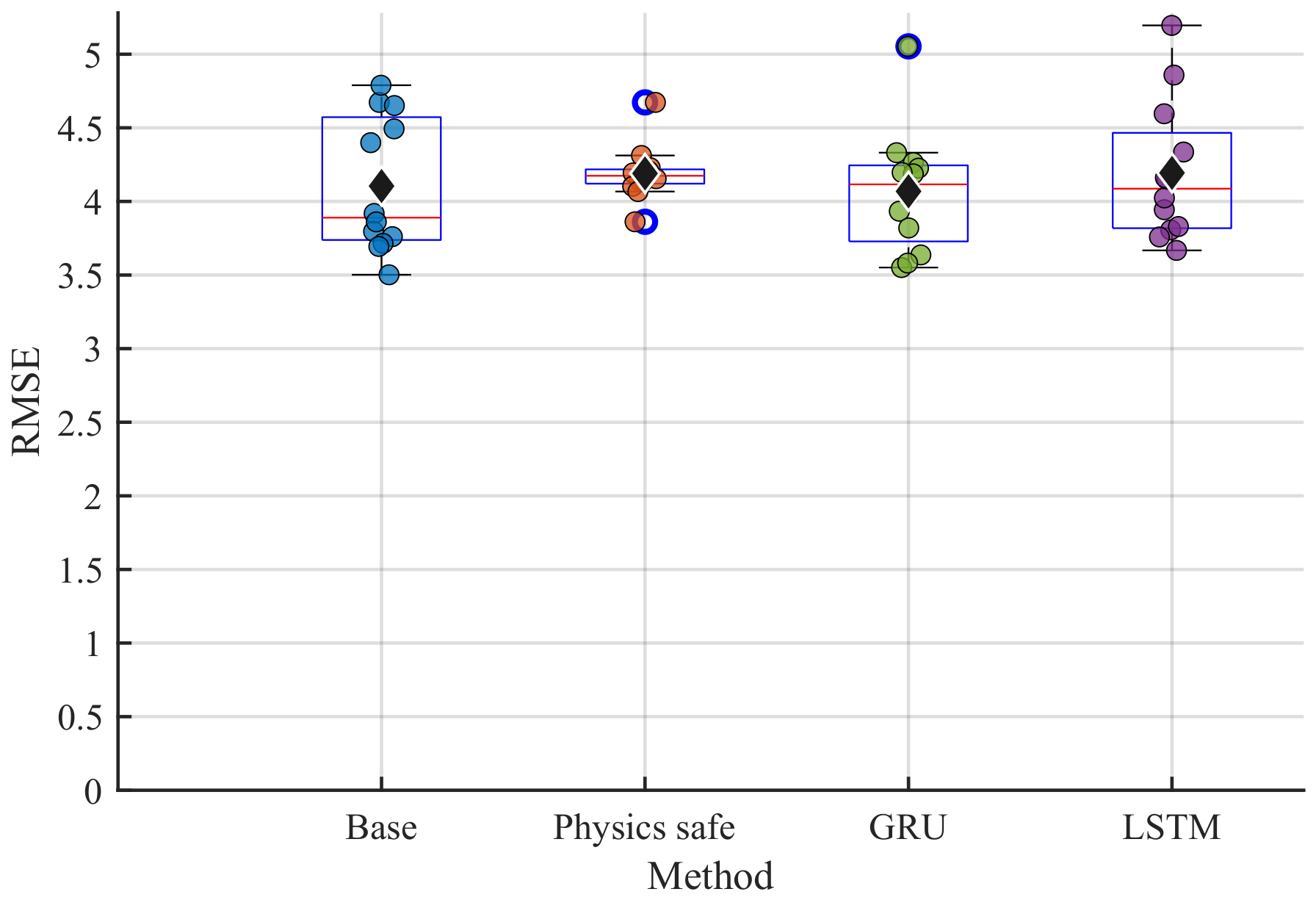
Dataset 8 is used as the main independent comparison dataset. It is not used for training, hyperparameter tuning, validation selection, or checkpoint selection. In this evaluation, the frozen Base, Physics-safe, GRU, and LSTM models are compared across 12 random training seeds. In addition, UKF-based observers are included as conventional model-based references. The results of the neural-network-based methods are reported in

Table 7. Independent comparison results on Dataset 8.

Method	n	Mean RMSE	Std.	Median RMSE	Min. RMSE	Max. RMSE
GRU	12	4.068812	0.416127	4.115981	3.550887	5.053330
Base	12	4.104517	0.459171	3.889701	3.501794	4.789344
Physics-safe	12	4.190386	0.187440	4.174233	3.861834	4.672852
LSTM	12	4.193817	0.473968	4.086539	3.667320	5.195838

and Figure 3.

As shown in Table 7 and Figure 3, GRU achieves the lowest mean RMSE on Dataset 8, followed by Base. The mean RMSE of Physics-safe is slightly higher than those of GRU and Base and is close to that of LSTM. Therefore, Dataset 8 does not support the conclusion that Physics-safe is the best method in terms of mean RMSE.

However, Physics-safe achieves the lowest inter-seed RMSE standard deviation, with a value of 0.187440. This value is clearly lower than those of Base, GRU, and LSTM. The box-and-scatter distribution in Figure 3 also shows that the Physics-safe results are more concentrated across different random training seeds. This indicates that the proposed validation-protected physics-consistent training strategy improves training stability, even though it does not minimize the mean RMSE on this independent comparison dataset.

The paired comparison results further support this interpretation. Physics-safe obtains 4 wins, 1 tie, and 7 losses against Base; 4 wins, 0 ties, and 8 losses against GRU; and 5 wins, 0 ties, and 7 losses against LSTM. The corresponding two-sided sign tests do not reach statistical significance. Therefore, the appropriate conclusion for Dataset 8 is that Physics-safe is not statistically superior in mean accuracy, but it exhibits the lowest inter-seed variability among the neural estimators.

For the conventional model-based references, the fixed-configuration UKF and enhanced UKF obtain RMSE values of approximately 22.61 and 22.51 on Dataset 8, respectively. Both observers retained their development-stage motor-model parameters and process- and measurement-covariance settings during the frozen Dataset 8 evaluation. Dataset 8 combines a wide-range, time-varying speed profile with a strong load change. Under these conditions, unmodeled load dynamics, model mismatch, and nonstationary effective disturbances depart from the behavior represented by the fixed model and covariance settings, providing a plausible explanation for the observed degradation. This comparison therefore characterizes the selected fixed-configuration UKF references under the present protocol and should not be interpreted as evidence that adaptive, operating-point-dependent, or differently tuned UKF designs are intrinsically inferior.

5.5. Supplementary Disturbance Evaluation

To further evaluate the performance boundary of the frozen models under additional disturbance conditions, Dataset 9, Dataset 10, and Dataset 11 are used as supplementary robustness test datasets. Dataset 9 corresponds to the load disturbance scenario, Dataset 10 corresponds to the parameter mismatch scenario, and Dataset 11 corresponds to the noise disturbance scenario. These datasets are evaluated only after the models are frozen, and they are not used for training, hyperparameter tuning, validation selection, or checkpoint selection. The results are reported in

Table 8. Supplementary disturbance evaluation results on Dataset 9, Dataset 10, and Dataset 11.

Dataset	Method	n	Mean RMSE	Std.	Median RMSE
Dataset 9	Base	12	3.181568	0.485033	3.071856
Dataset 9	Physics-safe	12	3.365535	0.114937	3.398940
Dataset 9	GRU	12	3.574229	0.607225	3.512547
Dataset 9	LSTM	12	3.738144	1.128521	3.217360
Dataset 10	Base	12	3.099820	0.472011	3.024093
Dataset 10	Physics-safe	12	3.285409	0.125954	3.330043
Dataset 10	GRU	12	3.680723	0.635647	3.704331
Dataset 10	LSTM	12	3.954889	1.162729	3.356234
Dataset 11	Base	12	2.905583	0.510108	2.747812
Dataset 11	Physics-safe	12	3.068920	0.159604	3.079254
Dataset 11	GRU	12	3.180535	0.540138	3.249135
Dataset 11	LSTM	12	3.443169	0.785313	3.027739

.

As shown in Table 8, Base achieves the lowest mean RMSE in all three supplementary disturbance scenarios. This indicates that the baseline probabilistic neural estimator has strong mean-accuracy performance under the present disturbance settings. Therefore, these results do not support the claim that Physics-safe is the mean-RMSE-optimal method under the supplementary disturbance conditions.

Nevertheless, Physics-safe achieves the lowest inter-seed RMSE standard deviation on Dataset 9, Dataset 10, and Dataset 11, with values of 0.114937, 0.125954, and 0.159604, respectively. These values are lower than those of Base, GRU, and LSTM in the corresponding scenarios. This result indicates that the main advantage of Physics-safe under load disturbance, parameter mismatch, and noise disturbance is its reduced sensitivity to random training seeds.

Compared with GRU and LSTM, Physics-safe also obtains lower mean RMSE values in all three supplementary disturbance datasets. In particular, under the parameter mismatch scenario of Dataset 10, Physics-safe shows a clear numerical advantage over GRU. However, the sign test does not reach statistical significance. Therefore, these results are described as numerical trends and stability advantages rather than statistically significant superiority claims.

5.6. Probabilistic Output Evaluation

To directly evaluate the probabilistic output of the proposed estimator, the Gaussian NLL, empirical 95% PICP, and 95% MPIW defined in Section 4.7 are calculated on Datasets 8–11. All results are obtained from the same 12 frozen Physics-safe checkpoints used in the point-estimation analysis. No retraining, fine-tuning, variance rescaling, post hoc calibration, hyperparameter adjustment, or checkpoint reselection is performed.

As shown in

Table 9. Probabilistic output evaluation of the frozen Physics-safe estimator on Datasets 8–11. Values are reported as mean ± sample standard deviation over 12 frozen checkpoints.

Dataset	Gaussian NLL	95% PICP (%)	95% MPIW ($\mathbf{rad}/\mathbf{s}$)
Dataset 8	$3.238760\pm 0.009637$	$100.000\pm 0.000$	$35.910175\pm 0.020819$
Dataset 9	$3.201293\pm 0.004556$	$100.000\pm 0.000$	$35.903252\pm 0.008959$
Dataset 10	$3.198176\pm 0.004914$	$100.000\pm 0.000$	$35.904916\pm 0.011514$
Dataset 11	$3.189982\pm 0.005664$	$100.000\pm 0.000$	$35.903264\pm 0.008983$

, the Gaussian NLL values remain similar across the four frozen test datasets. The nominal 95% prediction intervals achieve an empirical coverage of 100% on every dataset. However, the corresponding mean interval widths are approximately $35.9\mathrm{rad}/\mathrm{s}$ and vary only slightly across datasets and random seeds. This near-constant width is consistent with the implemented lower log-variance clipping bound. Specifically, because the log-variance output is clipped at $-8$ in the normalized coordinates and the physical speed scale is $500\mathrm{rad}/\mathrm{s}$, the minimum physical standard deviation is $500\exp (-4)\approx 9.16\mathrm{rad}/\mathrm{s}$, corresponding to a nominal 95% interval width of approximately $2\times 1.96\times 500\exp (-4)\approx 35.90\mathrm{rad}/\mathrm{s}$. The observed MPIW values therefore lie close to this theoretical lower bound, indicating that the present numerical-stability clipping limits interval sharpness. Consequently, the complete empirical coverage should not be interpreted as evidence of well-calibrated uncertainty. Instead, the frozen prediction intervals are conservative and exhibit limited sharpness and limited heteroscedastic variation under the present evaluation protocol.

These results directly characterize the previously unevaluated probabilistic output of the estimator. They support the description of the network as a Gaussian probabilistic estimator because it produces and is evaluated through an explicit predictive distribution, but they do not support a claim of accurately calibrated predictive uncertainty. Calibration and interval sharpness therefore remain limitations of the current frozen model.

5.7. Auxiliary Residual-Compensation Diagnosis on Dataset 9

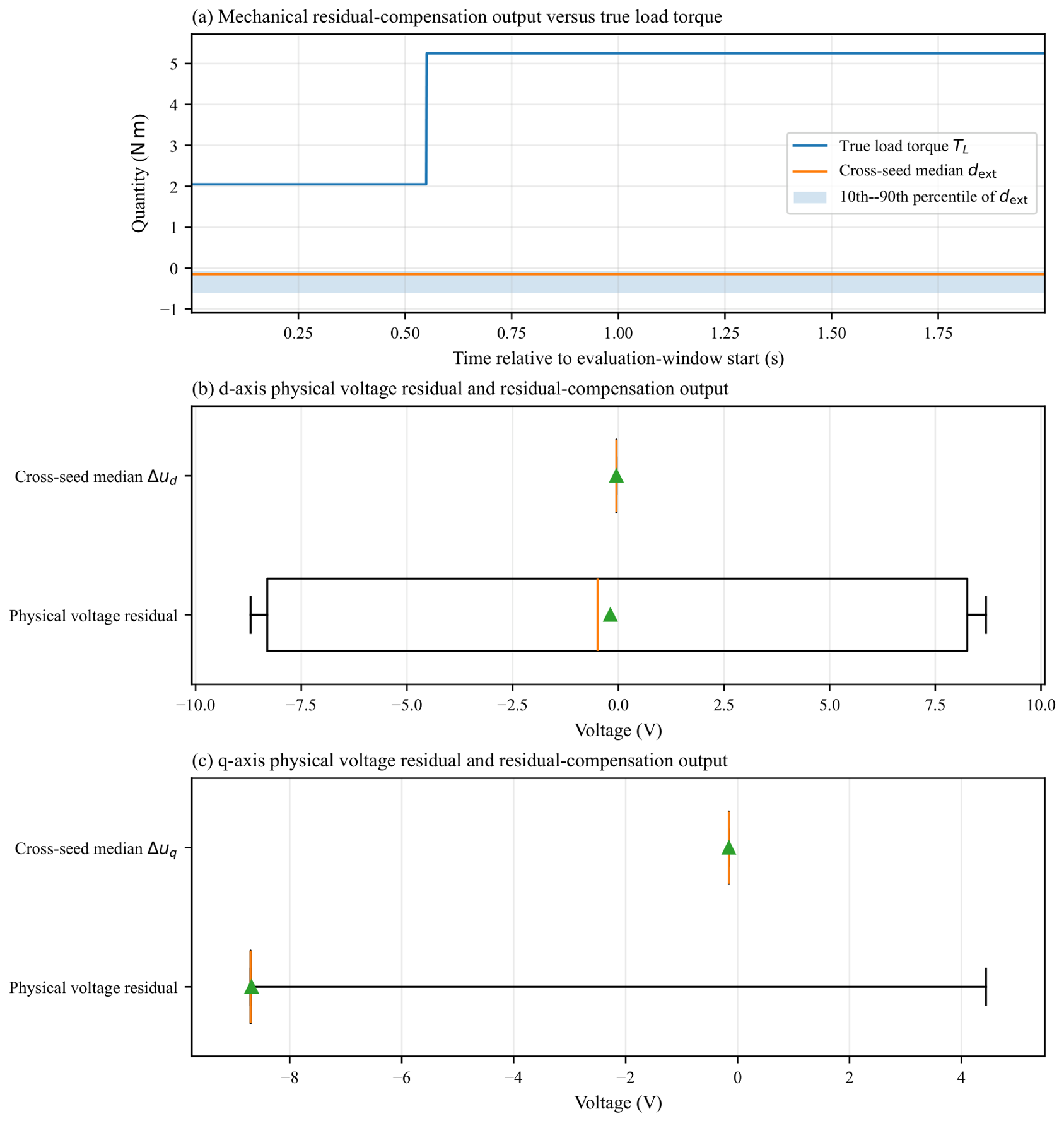
To examine the physical plausibility of the internally predicted auxiliary variables, an additional offline diagnosis is conducted on Dataset 9, which contains the dedicated load-torque change. The same 12 frozen Physics-safe checkpoints are used. The true load torque and actual d/q-axis voltages are loaded only after all recursive model inference has been completed and are used exclusively as offline physical references. For this offline diagnostic, the physical d- and q-axis voltage residuals are defined as $u_d^{\mathrm{actual}}-u_d^{\mathrm{cmd}}$ and $u_q^{\mathrm{actual}}-u_q^{\mathrm{cmd}}$, respectively; the box plots in Figure 4b,c summarize the 19,999 scored time samples. They are not supplied to the estimator as input signals, and no retraining, post hoc scaling, sign reversal, smoothing, or favorable seed selection is performed.

As shown in Figure 4, the true load torque changes from $2.05$ to $5.25\mathrm{N}\mathrm{m}$, whereas the cross-seed median mechanical residual-compensation output $d_{\mathrm{ext}}$ remains close to $-0.1463\mathrm{N}\mathrm{m}$ with a temporal sample standard deviation of only $7.36\times {10}^{-5}\mathrm{N}\mathrm{m}$. Similarly, the cross-seed median values of $\Delta u_{d,k}$ and $\Delta u_{q,k}$ remain close to $-0.0463\mathrm{V}$ and $-0.1558\mathrm{V}$, respectively. In contrast, the physical d-axis voltage residual has a temporal sample standard deviation of $7.2878\mathrm{V}$, while the physical q-axis voltage residual has a mean of $-8.6834\mathrm{V}$ and a temporal sample standard deviation of $0.3276\mathrm{V}$.

Consequently, the present frozen-output diagnosis does not support a one-to-one interpretation of $d_{\mathrm{ext},k}$, $\Delta u_{d,k}$, and $\Delta u_{q,k}$ as direct estimates of the true load torque or inverter-voltage errors. These quantities are therefore interpreted as internally predicted auxiliary residual-compensation variables that provide degrees of freedom within the physics-consistency losses. Their individual physical identifiability is not established by the current unsupervised formulation.

5.8. Cross-Dataset Summary

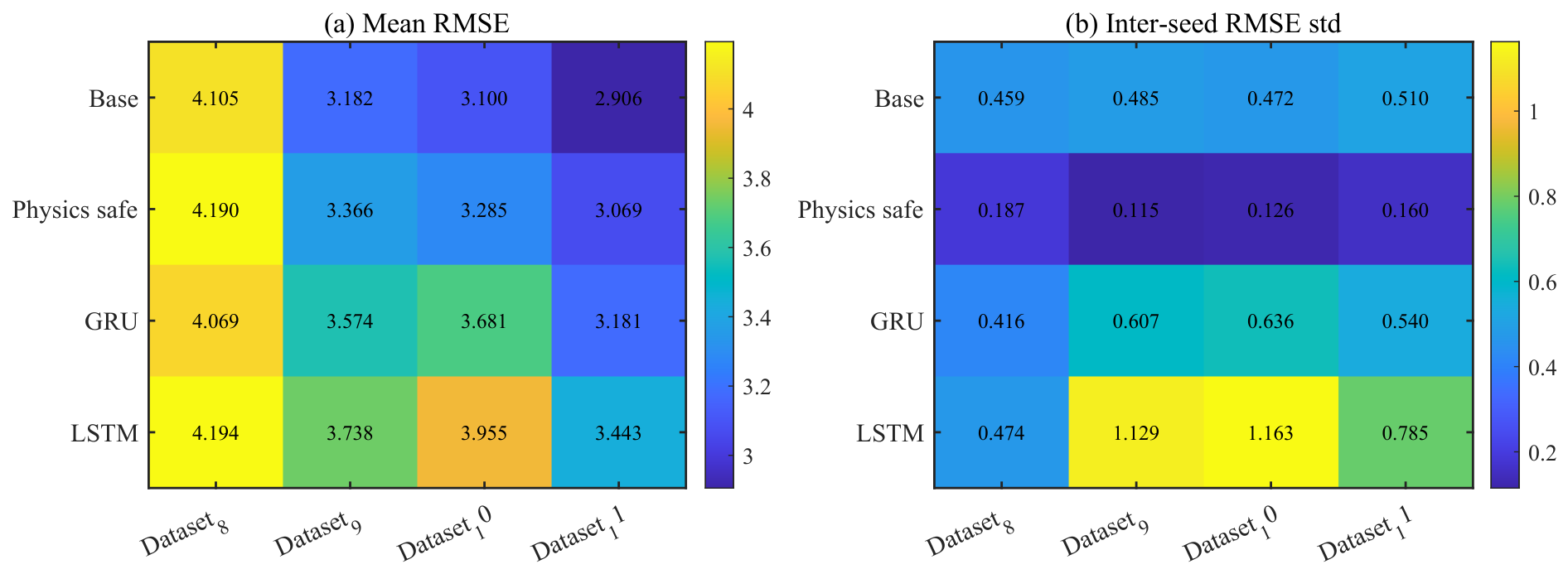
To further summarize the behavior of different methods across multiple frozen test scenarios, this subsection compares the mean RMSE and inter-seed RMSE standard deviation over Dataset 8, Dataset 9, Dataset 10, and Dataset 11. Figure 5 visualizes the accuracy and stability trends across the four frozen test datasets.

As shown in Figure 5, the method with the lowest mean RMSE varies across different test scenarios. GRU achieves the lowest mean RMSE on Dataset 8, whereas Base achieves the lowest mean RMSE on Dataset 9, Dataset 10, and Dataset 11. This indicates that the mean-accuracy advantage is not concentrated in a single method across all frozen test datasets. In contrast, Physics-safe consistently achieves the lowest inter-seed RMSE standard deviation across the four frozen test datasets, suggesting a more stable error distribution under different random training seeds.

The macro-average results over Dataset 8 to Dataset 11 are summarized in

Table 10. Cross-dataset macro-average results over Dataset 8 to Dataset 11.

Method	Mean RMSE	RMSE Standard Deviation
Base	3.322872	0.481581
Physics-safe	3.477563	0.146984
GRU	3.626075	0.549784
LSTM	3.832505	0.887633

.

As shown in Table 10, Base achieves the lowest macro-average mean RMSE over the four frozen test datasets, with a value of 3.322872. Physics-safe ranks second in macro-average mean RMSE, followed by GRU and LSTM. This result confirms that the proposed physics-consistent and validation-protected training strategy does not guarantee the lowest mean estimation error under all test scenarios.

However, Physics-safe achieves the lowest macro-average RMSE standard deviation, with a value of 0.146984. This value is substantially lower than those of Base, GRU, and LSTM. Therefore, the main advantage of Physics-safe lies in reducing the performance variation caused by random training seeds rather than minimizing the mean RMSE in every scenario.

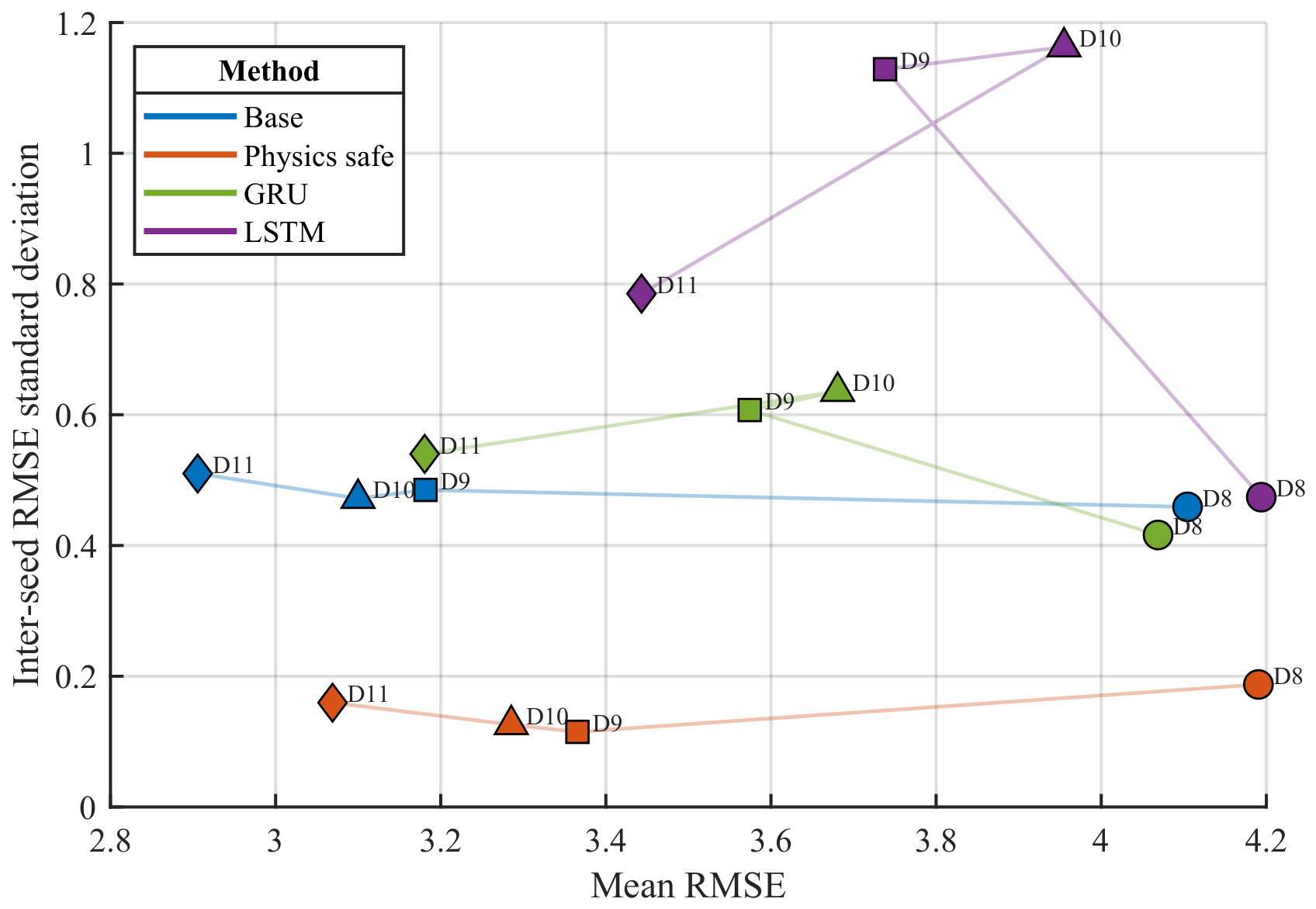
Figure 6 further illustrates the relationship between mean estimation accuracy and inter-seed stability.

The accuracy–stability distribution in Figure 6 provides a complementary interpretation of the results. Base is closer to the low-mean-error region in several supplementary disturbance scenarios, whereas Physics-safe is consistently located in a lower-standard-deviation region. This pattern supports the positioning of Physics-safe as a stability-enhanced neural speed estimator rather than a universally mean-error-optimal estimator.

Overall, the cross-dataset analysis shows that mean estimation accuracy and inter-seed stability should be considered separately when evaluating neural speed estimators for PMSM drives. A method with the lowest average error in one scenario may not provide the most reproducible training behavior across random seeds. Under the present frozen evaluation protocol, Physics-safe mainly improves reproducibility and inter-seed stability.

5.9. Computational Feasibility

The timing benchmark was conducted on a 64-bit Windows 11 system equipped with an Intel Core i5-10200H CPU, comprising four physical cores and eight logical processors, and approximately 16 GB of system memory. The frozen estimator was exported to the ONNX format and executed using ONNX Runtime 1.23.2 with the CPU Execution Provider. To reduce variability caused by runtime thread scheduling, both the intra-operation and inter-operation thread counts were fixed to one. No model training, parameter retuning, checkpoint selection, or dataset access was performed during the timing measurements.

The frozen Physics-safe estimator contains 34,437 trainable parameters, corresponding to approximately 134.5 KiB of raw float32 weights. Physics-consistent residuals and validation-protected checkpoint selection are used only during training and model selection. Therefore, Physics-safe and its paired Base estimator have the same online neural network architecture, parameter count, inference graph, and raw weight storage. Electrical power consumption and cross-platform embedded resource usage were not measured in the present benchmark.

Table 11. CPU inference-time benchmark of the frozen Physics-safe estimator.

Timing Scope	Mean Latency ($\mathsf{\mu }\mathbf{s}/\mathbf{Step}$)	SD Across 20 Repeat Means ($\mathsf{\mu }\mathbf{s}$)	95th Pct. Across 20 Repeat Means ($\mathsf{\mu }\mathbf{s}/\mathbf{Step}$)	Deadline-to-Latency Ratio (×)
Preallocated ONNX
Runtime call	34.911	0.343	35.303	2.864×
Complete recursive
estimator step	40.154	0.403	40.793	2.490×

Note: Each repeat contained 20,000 timed estimator steps after 5000 warm-up steps. The standard deviation and the 95th percentile were calculated across the 20 repeat-level mean latencies, rather than across all individual estimator steps.

reports the measured execution time of the frozen Physics-safe estimator. The preallocated ONNX Runtime session call required a mean latency of $34.911\mathsf{\mu }\mathrm{s}$ per estimator step. The standard deviation across the 20 repetition means was $0.343\mathsf{\mu }\mathrm{s}$, and the 95th-percentile repetition mean was $35.303\mathsf{\mu }\mathrm{s}$.

When input-buffer updating, output retrieval, and recursive feedback of the estimated speed were additionally included, the complete recursive estimator step required a mean latency of $40.154\mathsf{\mu }\mathrm{s}$. The standard deviation across the repetition means was $0.403\mathsf{\mu }\mathrm{s}$, and the 95th-percentile repetition mean was $40.793\mathsf{\mu }\mathrm{s}$.

Both the mean and the 95th-percentile repetition mean remained below the $100\mathsf{\mu }\mathrm{s}$ sampling period. The complete recursive estimator step occupied approximately $40.2\%$ of the sampling interval and yielded a deadline-to-latency ratio of approximately $2.49$.

These measurements support the computational feasibility of the frozen estimator in the tested CPU and ONNX Runtime environment. However, the benchmark covers only the estimator execution. It does not constitute hard-real-time certification of a complete embedded motor-drive controller because current-control computation, data acquisition, PWM updating, communication, interrupt handling, and target-controller scheduling overhead were not included.

5.10. Method Boundary Discussion

The experimental results show that the proposed Physics-safe estimator mainly improves the stability of neural speed estimation rather than guaranteeing the lowest mean RMSE in every test scenario. The physics-consistent losses constrain the estimator according to basic PMSM dynamics, while the validation-protected checkpoint selection mechanism reduces the risk of using a physics-trained checkpoint when it degrades validation performance. These two components jointly help reduce inter-seed performance variation.

At the same time, the results also indicate that physics-consistent training does not necessarily reduce the mean estimation error. When the Base model already fits the current data distribution well, additional physical residuals may introduce a trade-off between mean accuracy and inter-seed stability. Therefore, Physics-safe should not be described as a universally mean-error-optimal estimator. A more appropriate interpretation is that it is a stability-enhanced neural speed estimation method for sensorless PMSM drives.

Several limitations should also be acknowledged. First, all formal evaluations are based on the current PMSM simulation model and frozen data generation protocol. The results demonstrate the behavior of the proposed method under the present simulation conditions, but they should not be directly generalized to experimental motor test benches or hardware-in-the-loop platforms without further validation. Second, Dataset 9, Dataset 10, and Dataset 11 cover load disturbance, parameter mismatch, and noise disturbance scenarios, but they still represent a limited set of disturbance combinations. More diverse operating conditions and uncertainty sources should be investigated in future work. Third, the term “safe” refers to validation-performance degradation protection and does not constitute formal safety certification in the control-theoretic sense. Fourth, the frozen probabilistic outputs should not be interpreted as well-calibrated uncertainty estimates. Although the nominal 95% prediction intervals achieve 100% empirical coverage on Datasets 8–11, their mean widths remain approximately $35.9\mathrm{rad}/\mathrm{s}$ and vary only slightly across datasets and random seeds. The intervals are therefore conservative and exhibit limited sharpness under the present frozen evaluation protocol.

Fifth, the auxiliary residual-compensation variables are not directly supervised as estimates of the true load torque or physical inverter-voltage errors. The Dataset 9 offline diagnosis does not support a one-to-one physical interpretation of these outputs. They should therefore be understood as internal residual-compensation degrees of freedom within the physics-consistency training formulation rather than as validated physical observers. Future work should investigate uncertainty calibration using a separate development-only calibration set and should introduce explicit supervision or identifiability constraints if direct physical-quantity estimation is required.

Overall, the experimental results support the conclusion that Physics-safe improves the reproducibility and inter-seed stability of neural PMSM speed estimation under the present evaluation protocol. Its practical value lies in reducing the performance variation caused by random training seeds and providing a more stable estimator under disturbance scenarios. Several boundaries of the present evidence should be emphasized. First, all estimation-accuracy and disturbance-robustness results were obtained under the frozen simulation protocol; no hardware-in-the-loop or physical motor-drive experiment was conducted. Second, the loss-weight sensitivity analysis was performed only on the Dataset 4 validation subset using three development seeds and should therefore be interpreted as a local sensitivity characterization rather than evidence of globally optimal hyperparameters. Third, the inference-time benchmark measures only the frozen estimator under the specified desktop CPU and ONNX Runtime configuration and excludes current-control computation, data acquisition, PWM updating, communication, interrupt handling, and target-controller scheduling overhead. Finally, the validation-protected checkpoint rule limits validation-stage degradation relative to the paired baseline checkpoint, but it does not provide a formal control-theoretic safety guarantee or ensure superiority under every unseen operating condition. Accordingly, the results support improved reproducibility and validation-protected model selection within the tested protocol, rather than universal accuracy, robustness, or hard-real-time guarantees.

6. Conclusions

This study developed a validation-protected physics-consistent probabilistic neural estimator for sensorless PMSM speed estimation. The estimator combines a probabilistic data-fitting objective with mechanical consistency, electrical consistency, and regularization of the auxiliary residual-compensation variables, while a validation-protected checkpoint rule selects between the paired baseline and physics-trained candidates for each random seed.

The development-stage ablation results on Dataset 4 show that the mechanical consistency loss, electrical consistency loss, and regularization term each contribute to constraining the estimator, because removing an individual component causes observable performance degradation. The subsequent one-factor-at-a-time sensitivity analysis further shows that the physics-trained checkpoint is sensitive to both the loss-weight configuration and the random training seed. Across the 21 development-stage runs, the physics-trained checkpoint was selected in 12 cases, whereas the baseline checkpoint was retained in 9 cases. These results do not identify a globally optimal loss-weight combination; instead, they demonstrate the practical role of validation protection when approximate physical constraints and multi-objective optimization produce seed-dependent outcomes.

Under the locked holdout protocol on Dataset 7, Physics-safe reduced the mean RMSE from 3.415 for Base to 3.277 and reduced the inter-seed RMSE standard deviation from 0.290 to 0.052. The independently generated Dataset 8 and the supplementary load disturbance, parameter mismatch, and input-noise tests on Datasets 9–11 further show that the proposed method should not be interpreted as universally mean-error optimal. Its more consistent advantage is the reduction in performance variation across random seeds and the resulting improvement in training reproducibility under the tested operating conditions.

Additional frozen-output diagnostics further clarify the interpretation of the probabilistic and auxiliary outputs. Across Datasets 8–11, the Gaussian NLL values range from $3.190$ to $3.239$, while the nominal 95% prediction intervals achieve 100% empirical coverage with mean widths of approximately $35.9\mathrm{rad}/\mathrm{s}$. The uncertainty output is therefore conservative and exhibits limited sharpness rather than being well calibrated. Moreover, the Dataset 9 offline diagnosis does not establish a one-to-one correspondence between the auxiliary residual-compensation variables and the true load torque or physical inverter-voltage errors. These auxiliary outputs are more appropriately interpreted as internal residual-compensation variables within the physics-consistency training formulation rather than as validated physical observers.

The computational benchmark also indicates that the frozen estimator is executable within the adopted $100\mathsf{\mu }\mathrm{s}$ sampling interval on the specified desktop CPU and ONNX Runtime configuration. The complete recursive estimator step required a mean latency of $40.154\mathsf{\mu }\mathrm{s}$, and its 95th-percentile repetition mean was $40.793\mathsf{\mu }\mathrm{s}$, corresponding to a deadline-to-latency ratio of approximately $2.49$. This result supports computational feasibility for the tested estimator implementation, but it does not constitute hard-real-time certification of a complete embedded motor-drive controller.

Overall, the main contribution of the proposed framework is not a guarantee of the lowest mean RMSE in every scenario, but a validation-protected mechanism for exploiting approximate physical knowledge while limiting validation-stage degradation relative to the paired baseline checkpoint. Within the frozen simulation and evaluation protocol, this design improves the reproducibility and inter-seed stability of neural PMSM speed estimation. Future work should evaluate the method through hardware-in-the-loop and physical motor-drive experiments, investigate adaptive or normalized loss balancing, and assess execution time and closed-loop behavior on embedded target controllers.