A Multi-Fault Diagnosis Method for Cylindrical Roller Bearings Based on RSNGO-Optimized VMD and CNN-BiLSTM-SAT

Abstract

To address the problems of severe feature coupling, difficult fault information extraction, and insufficient recognition accuracy for cylindrical roller bearings under multiple fault conditions, this paper proposes a multi-fault pattern recognition method based on a Northern Goshawk Optimization algorithm improved by refraction opposition-based learning and the sine–cosine algorithm (RSNGO). The RSNGO is used to optimize variational mode decomposition (VMD) and a convolutional neural network–bidirectional long short-term memory–self-attention (CNN–BiLSTM–SAT) network. First, RSNGO adaptively optimizes the number of decomposition modes and the penalty factor of VMD, and selects the optimal intrinsic mode function (IMF) components, from which time-domain statistical features are extracted to construct the sample set. Then, a CNN–BiLSTM–SAT diagnostic network is constructed, and RSNGO is employed to jointly optimize its key hyperparameters, including convolution kernel size, number of convolution kernels, number of BiLSTM hidden units, and initial learning rate. In this network, CNN extracts local features, BiLSTM models temporal dependencies, and the self-attention mechanism enhances the representation of critical fault features. Finally, the constructed feature samples are input into the optimized network to realize multi-fault pattern recognition of cylindrical roller bearings. Experimental results demonstrate that the proposed method effectively improves the separability and recognition accuracy of multi-fault features, exhibits strong robustness and generalization capability under complex operating conditions, and provides an effective solution for intelligent bearing fault diagnosis.

1. Introduction

Fault signals generated by cylindrical roller bearings are often characterized by nonstationary behavior, strong noise contamination, and complex fault coupling, posing significant challenges to accurate feature extraction. Despite the widespread adoption of deep learning techniques in bearing fault diagnosis, their performance remains constrained by limited generalization ability and high dependence on labeled training data, particularly under cross-condition, small-sample, and noisy operating environments [1,2]. From the perspective of signal processing, variational mode decomposition (VMD), proposed by Dragomiretskiy et al. [3], adaptively decomposes nonstationary signals into a set of narrow-band mode components, thereby enhancing the separability of fault-induced impulsive features. Owing to its strong resistance to mode mixing and its clear theoretical constraints, VMD has been widely adopted for bearing fault feature extraction in recent years. Nevertheless, the decomposition performance of VMD is highly sensitive to parameters such as the number of modes $K$ and the penalty factor $\alpha$. Improper parameter settings may lead to under-decomposition or over-decomposition, thereby degrading subsequent diagnostic performance. To address this issue, Zhou et al. [4] proposed an adaptive parameter range selection strategy for VMD under strong background noise; Li et al. [5] developed a bearing fault diagnosis model that combines adaptive VMD with a sparrow search algorithm optimized probabilistic neural network; and Zhou et al. [6] introduced whale optimization into VMD parameter tuning. These studies demonstrate that intelligent optimization algorithms can effectively reduce reliance on manual experience in VMD parameter selection, which also provides methodological motivation for the RSNGO (Refraction Opposition-Based Learning and Sine–Cosine Search Strategy Northern Goshawk Optimization)—based VMD optimization adopted in this work. Regarding optimization algorithms, Dehghani et al. [7] proposed the Northern Goshawk Optimization (NGO) algorithm, which mimics the hunting behavior of northern goshawks and balances global exploration with local exploitation. Liang et al. [8] subsequently developed an enhanced NGO by improving the search strategy, thereby further improving its ability to solve complex optimization problems. These studies suggest that population-based metaheuristic algorithms with strong global search capability are well suited to continuous parameter optimization problems, providing a theoretical basis for integrating reflective-refraction learning and sine–cosine search strategies into the NGO framework to construct RSNGO for VMD parameter optimization. In terms of feature learning, convolutional neural networks (CNNs) remain one of the most important local feature extraction backbones in bearing fault diagnosis, but their application has evolved from single-scale convolution toward multiscale modeling and attention-based reweighting. Huang et al. [9] proposed CA-MCNN, which combines multiscale convolution with channel attention. By using multiscale pooling to enhance information representation and adaptively assign feature weights, the network improves the extraction of critical fault-related information. For temporal modeling, Song et al. [10] developed an improved CNN-BiLSTM network for bearing fault diagnosis under multiple operating conditions and limited training samples, demonstrating that the local pattern extraction capability of CNNs and the bidirectional temporal dependency modeling capability of BiLSTM are highly complementary, particularly for nonstationary vibration signals under varying operating conditions. Furthermore, Huang et al. [11] constructed a dual-channel CNN-BiLSTM fusion model with attention for aero-engine bearing fault diagnosis, showing that introducing an attention mechanism in complex scenarios helps emphasize fault-related features while suppressing redundant information. Siddique et al. [12] proposed a hybrid framework combining CWT, MHSA, BiLSTM, and a one-dimensional convolutional residual network, further indicating that the synergy between multi-head self-attention and spatiotemporal feature extraction networks can more effectively learn discriminative information from nonstationary and nonlinear signals. In addition, Fu et al. [13] proposed a parallel CNN-LSTM model to extract vibration features from both spatial and temporal dimensions; Han et al. [14] proposed a CNN-LSTM-GRU network to improve diagnostic performance under complex operating conditions; Deng et al. [15] employed HSGWO to optimize a CNN-BiLSTM network, thereby enhancing its ability to capture complex patterns and improve robustness; Dong et al. [16] developed a one-dimensional improved attention-enhanced CNN combined with empirical wavelet transform to improve feature focusing under noisy conditions; Zhao et al. [17] proposed a multiscale CNN combined with BiLSTM and attention for multi-condition bearing fault identification; and Zhang et al. [18] presented an attention-activated network for noisy environments, further verifying the effectiveness of attention mechanisms in weak fault recognition. Collectively, these studies indicate that integrating convolutional structures, temporal modeling, and attention mechanisms has become an important direction for improving fault diagnosis performance in complex scenarios. Meanwhile, to address the issues of limited training samples and insufficient feature representation capability, various enhancement strategies have also been proposed. Wang et al. [19] introduced a CNN-based fault diagnosis framework enhanced by variational autoencoders (VAEs) to improve data representation quality, while Zhang et al. [20] proposed a few-shot transfer learning-based bearing fault diagnosis method to alleviate sample scarcity and domain shift across different datasets. These works indicate that, in practical industrial scenarios, relying solely on raw signals and fixed classifiers is often insufficient to simultaneously achieve robustness and generalization. More effective signal decomposition, feature enhancement, and deep feature modeling mechanisms are therefore required.

Building upon the aforementioned research foundation, this paper proposes a bearing multi-fault diagnosis method that integrates RSNGO-based optimization of VMD and CNN-BiLSTM-SAT networks: First, RSNGO is employed to automatically optimize key parameters of VMD for superior modal decomposition results; then, multidimensional time-domain features are constructed from the optimized IMF; and finally, the RSNGO-enhanced CNN-BiLSTM-SAT hybrid network enables local pattern extraction, long-range dependency modeling, and critical feature enhancement, thereby improving multi-fault identification accuracy and generalization performance under complex operating conditions.

2. Basic Theory

2.1. Northern Goshawk Algorithm Combining Refractive Reverse Learning and Sine–Cosine

Northern Goshawk Optimization (NGO) is a novel swarm intelligence algorithm originally proposed by Dehghani et al. [7], which simulates the hunting behavior of the northern goshawk. The algorithm achieves global exploration and local exploitation through two distinct phases, namely the attack phase and the chase phase. To address the issues of limited population diversity and the imbalance between exploration and exploitation in the original NGO algorithm, an improved version, termed RSNGO, is proposed. The enhanced algorithm incorporates refractive reverse learning [21] and a sine–cosine search strategy [22]. Specifically, refractive reverse learning is employed to generate a high-quality initial population, while the sine–cosine strategy is introduced to update individual positions during the exploration phase, thereby improving the balance between global exploration and local exploitation. The mathematical formulation of RSNGO is presented as follows.

Exploration phase: During the exploration phase, the northern goshawk initially scans the search area extensively. Once a potential prey target is identified, it evaluates the target before launching an attack. The corresponding mathematical expressions for prey identification and attack behaviors are given as follows:

$$P_a=X_l,a=1,2,\cdot \cdot \cdot \cdot N,l=1,2,\cdot \cdot \cdot \cdot ,N,l\ne a$$

(1)

$$x_{a,b}^{new,p_1}=\left\{\begin{array}{c}{x}_{a,b}+r(p_{a,b}-I{x}_{a,b}),F_{p_a}<F_a\\ x_{a,b}+r(p_{a,b}-x_{a,b}),F_{p_a}\ge F_a\end{array}\right.$$

(2)

$$X_a=\left\{\begin{array}{c}{X}_a^{new,p_1},F_a^{new,p_1}<F_a\\ X_a,F_a^{new,p_1}\ge F_a\end{array}\right.$$

(3)

where $P_a$ denotes the position of the a-th northern goshawk, N is the population size, and $l$ represents the position of another randomly selected individual. $x_{a,b}^{new,p_1}$ is the updated b-dimensional position of the northern goshawk a in the northern goshawk population, where b = 1, 2, …, D, and D is the total number of optimization variables. Similarly, $x_{a,b}$ represents the position of the a-th northern goshawk in the b-th dimension. r is a random number in the interval [0, 1], and I is a specific random number of 1 or 2. $F_{Pa}$ is the fitness value of the position of the predator a, and $F_a^{new,p_1}$ is the updated fitness value of the northern goshawk a.

Based on this, an inverse refraction learning mechanism is adopted to initialize the individual parameters of the Northern Goshawk Optimization algorithm, and a sine–cosine search strategy is used to replace the position update formula in the exploration phase of the original NGO algorithm, while optimizing the step size search factor. The specific formulas are as follows:

$$x_{a,b}^{\ast }={\displaystyle \frac{(h_b+l_b)}{2}}+{\displaystyle \frac{(h_b+l_b)}{2k^{\prime }}}+{\displaystyle \frac{x_{a,b}}{k^{\prime }}}$$

(4)

$$X_{a,b}^{t^{\prime }+1}=\left\{\begin{array}{c}{\omega }^{\prime }={\displaystyle \frac{e^{t^{\prime }/t_{\max }^{\prime }}-1}{e-1}}\\ {\omega }^{\prime }\cdot X_{a,b}^{t^{\prime }}+r_1^{\prime }\cdot \sin r_2^{\prime }\cdot |r_3^{\prime }\cdot X_{a,b}^{best}-X_{a,b}^{t^{\prime }}|,R_2^{\prime }<S{T}^{\prime }\\ {\omega }^{\prime }\cdot X_{a,b}^{t^{\prime }}+r_1^{\prime }\cdot \cos r_2^{\prime }\cdot |r_3^{\prime }\cdot X_{a,b}^{best}-X_{a,b}^{t^{\prime }}|,R_2^{\prime }\ge S{T}^{\prime }\end{array}\right.$$

(5)

where $x_{a,b}^{\ast }$ is the refractive reverse position; $h_b$ and $l_b$ are the minimum and maximum values of the b-dimensional position; $k^{\prime }$ is the scaling factor; $X_{a,b}^{t^{\prime }}$ and $X_{a,b}^{t^{\prime }+1}$ are the b-dimensional positions of the northern goshawk a in the northern goshawk population after by the $t^{\prime }$ and $t^{\prime }+1$ iterations of the update, respectively; and $X_{a,b}^{best}$ is the overall optimal position of the northern goshawk at present.

During the exploitation phase, when a northern goshawk locks onto its prey, the prey attempts to escape. The northern goshawk is capable of tracking its target in three-dimensional space at extremely high speeds during pursuit. Suppose the prey is located within a spherical region centered on the point of attack as the origin and with a radius of R, the mathematical formula for the development stage is

$$x_{a,b}^{new,p_2}=x_{a,b}+R(2r-1)x_{a,b}$$

(6)

$$R=0.02(1{\displaystyle -\frac{t^{\prime }}{t_{\max }^{\prime }}})$$

(7)

$$X_a=\left\{\begin{array}{c}{X}_a^{new,p_2},F_a^{new,p_2}<F_a\\ X_a,F_a^{new,p_2}\ge F_a\end{array}\right.$$

(8)

where $X_a^{new,p_2}$ is the new position of the northern goshawk a after the development phase update, $x_{a,b}^{new,p_2}$ is the b-dimensional position of the northern goshawk a after the development phase update, and $F_a^{new,p_2}$ is the fitness value of the northern goshawk a after the development phase update.

2.2. Variational Mode Decomposition

VMD was originally proposed by Dragomiretskiy and Zosso [3]. Unlike recursive algorithms such as EMD and its variants, VMD is a non-recursive mode decomposition algorithm capable of decomposing an input signal into K intrinsic mode functions $u_k(t)$ while determining their respective center frequencies and bandwidths to distinguish different modes. The core of the algorithm lies in constructing and solving a constrained variational model. The corresponding algorithmic procedure is as follows:

Before constructing the variational model, each mode $u_k(t)$ must undergo a Hilbert transform to modulate its spectrum to the corresponding baseband. The mathematical formulation is as follows:

$$F_k=\left[\left(\delta (t)+j/\pi t\right)*u_k(t)\right]e^{-j{\omega }_{k}t}$$

(9)

where j denotes the imaginary unit, $\delta (t)$ represents the Dirac delta function, $u_k(t)$ is the k-th intrinsic mode function, and ${\omega }_k$ is its corresponding center frequency.

Solving for the square of the L2 paradigm of the gradient of the modulated signal to estimate the bandwidth of each mode, the variational model is as follows:

$$\left\{\begin{array}{c}\min \{{\displaystyle \sum _{k=1}^K\left|\right|{\partial }_t[(\delta (t)+j/\pi t)*u_k(t)]e^{-j{\omega }_{k}t}|{|}_2^2\}}\\ s.t.{\displaystyle \sum _{k=1}^K{u}_k(t)=w(t)}\end{array}\right.$$

(10)

where ${\partial }_t$ is the function taking the partial derivative with respect to t and “*” is the convolution operation.

The variational model is transformed into an unconstrained variational model and then solved by introducing Lagrange multipliers $\lambda (t)$ and quadratic penalty factor $\alpha$ and determining the corresponding augmented generalized Lagrangian function as

$$\begin{array}{cc}\hfill L(\{u_k\},\{{\omega }_k\},\lambda )& =\alpha {\displaystyle \sum _{k=1}^K\left|\right|{\partial }_t}[(\delta (t)+j/\pi t)*u_k(t)]e^{-j{\omega }_{k}t}|{|}_2^2\hfill \\ \hspace{1em}& +||w(t)-{\displaystyle \sum _{k=1}^K{u}_k(t)}|{|}_2^2+\langle \lambda (t),w(t)-{\displaystyle \sum _{k=1}^K{u}_k(t)}\rangle \hfill \end{array}$$

(11)

where $L(\cdot )$ is the Lagrange function and $\lambda (t)$ is the Lagrange multiplier.

The alternating direction multiplier algorithm is used to continuously update the iterations of $u_k$, ${\omega }_k$, and $\lambda$ to obtain the optimal solutions including $u_k^{(n+1)}$, ${\omega }_k^{(n+1)}$, and ${\lambda }^{(n+1)}$. The iterative process continues until the convergence criterion defined in Equation (15) is satisfied; the iterative process is

$${\widehat{u}}_k^{(n+1)}(\omega )={\displaystyle \frac{\widehat{w}(\omega ){\displaystyle -\sum _{i<k}{\widehat{u}}_i^{(n+1)}(\omega )-{\displaystyle \sum _{i>k}{\widehat{u}}_i^n(\omega )+{\widehat{\lambda }}^n(\omega )/2}}}{1+2\alpha {(\omega -{\omega }_k^n)}^2}}$$

(12)

$${\omega }_k^{(n+1)}={\displaystyle \frac{{\displaystyle {\int }_0^{\infty }\omega {\left|{\widehat{u}}_k^{(n+1)}(\omega )\right|}^{2}d\omega }}{{\displaystyle {\int }_0^{\infty }{\left|{\widehat{u}}_k^{(n+1)}(\omega )\right|}^{2}d\omega }}}$$

(13)

$${\widehat{\lambda }}^{(n+1)}(\omega )={\widehat{\lambda }}^n(\omega )+\Gamma \left(\widehat{w}(\omega ){\displaystyle -\sum _{k=1}^K{\widehat{u}}_k^{(n+1)}(\omega )}\right)$$

(14)

$${\displaystyle \sum _k\frac{\parallel {\widehat{u}}_k^{(n+1)}-{\widehat{u}}_k^n{\parallel }_2^2}{\parallel {\widehat{u}}_k^n{\parallel }_2^2}}<\epsilon$$

(15)

where “^” denotes the Fourier transform, k represents the index of the decomposed mode, n denotes the iteration number of the VMD optimization process, $\Gamma$ is the noise tolerance limit, and $\epsilon$ represents the convergence accuracy.

2.3. Convolutional Neural Network

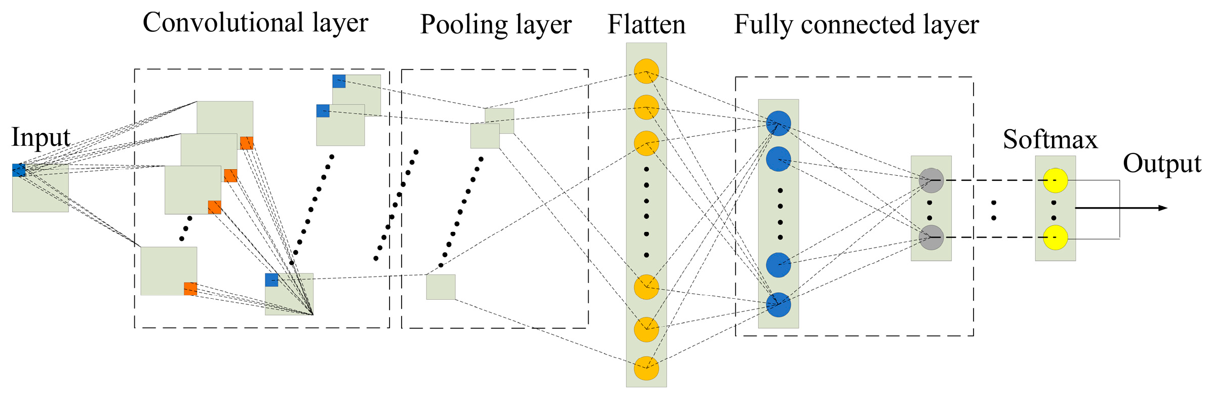
Convolutional neural network (CNN) [23], as a typical deep learning architecture, demonstrates significant advantages in computer vision tasks such as target detection. The structure of the CNN model is shown in Figure 1.

The network architecture mainly consists of three components: a convolutional layer for local feature extraction, a pooling layer for feature dimensionality reduction, and a fully connected layer for high-level feature integration and classification.

The convolutional layer is primarily responsible for extracting spatial information from the input features. The convolution operation can be expressed as follows:

$$x_j^l=f({\displaystyle \sum _{i=1}^M{k}_{ij}^l{x}_i^{l-1}+b_j^l})$$

(16)

where $x_j^l$ is the feature mapping number j in layer $l$, $k_{ij}^l$ is the convolution kernel in layer l, $x_i^{l-1}$ is the feature mapping number i in layer l − 1, $b_j^l$ is the bias of layer l, and $f(\cdot )$ is the activation function.

The pooling layer is utilized to perform downsampling, thereby reducing the dimensionality of the feature maps generated by the convolutional layer while preserving the most representative features. The pooling operation can be mathematically expressed as follows:

$$p_i^l(j)=\max \{q_i^l(t)\},(j-1)W^{\prime }+1\le t\le j{W}^{\prime }$$

(17)

where $p_i^l(j)$ is the pooling layer output value, $q_i^l(t)$ is the activation value of the neuron t in the feature i of the layer l, and $W^{\prime }$ is the convolution kernel width.

The fully connected layer primarily performs full connection and classification operations, flattens the features after pooling, and outputs classification results using the SoftMax function. The mathematical representation of the fully connected layer is as follows:

$$y_j^{l+1}=f({\displaystyle \sum _{i=1}{W}_{ij}^l}{X}_i^l+b_j^l)$$

(18)

where $y_j^{l+1}$ is the output of the neuron in layer l + 1, $W_{ij}^l$ is the weight of the neuron in layer l, and $X_i^l$ is the output of the neuron in layer l.

2.4. Bidirectional Long Short-Term Memory

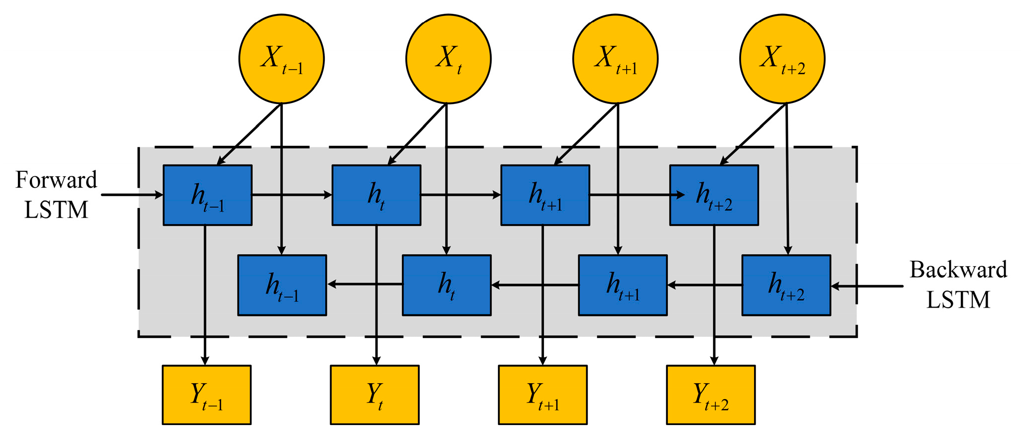
The bidirectional long short-term memory (BiLSTM) network [24] is an extension of the long short-term memory (LSTM) network [25]. Unlike the conventional LSTM, BiLSTM processes sequential data in both forward and backward directions, allowing it to capture contextual information from both past and future states. This bidirectional information flow enables the network to model temporal dependencies more effectively and extract richer time-domain characteristics from the input signals. The structure of the BiLSTM model is shown in Figure 2.

The timing signal is propagated to the corresponding LSTM layer through the BiLSTM input layer in the forward and backward directions, and the two LSTM layers are synchronized to generate the forward hidden state and the backward hidden state, respectively, and are spliced to obtain the final hidden state. Then, the bidirectional feature extraction of the timing signal is carried out, and the specific formula for the bidirectional output of the timing signal is as follows:

$$\overleftarrow{h_t}=f\left(\overleftarrow{{\omega }_x}\cdot X_t+\overleftarrow{h_{t-1}}\cdot \overleftarrow{{\omega }_h}+\overleftarrow{b_h}\right)$$

(19)

$$\overrightarrow{h_t}=f\left(\overrightarrow{{\omega }_x}\cdot X_t+\overrightarrow{h_{t-1}}\cdot \overrightarrow{{\omega }_h}+\overrightarrow{b_h}\right)$$

(20)

$$Y_t=f\left(\overrightarrow{{\omega }_y}\cdot \overrightarrow{h_t}+\overleftarrow{{\omega }_y}\cdot \overleftarrow{h_t}+b_y\right)$$

(21)

where $\overleftarrow{h_t}$ is the output after forward propagation, $\overrightarrow{h_t}$ is the output after backward propagation, and $Y_t$ is the output after forward and backward propagation.

2.5. Self-Attention

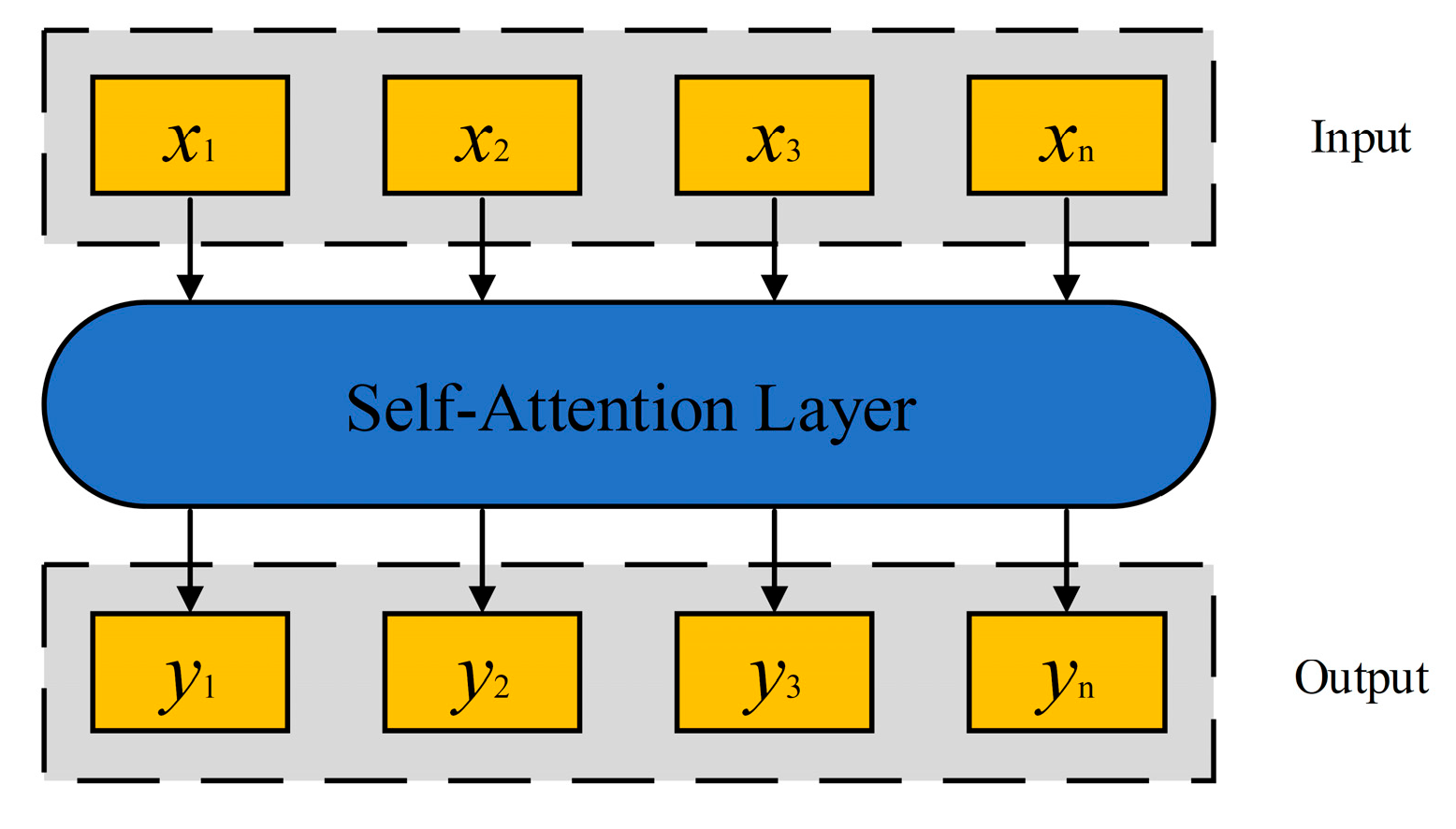
Self-attention (SAT) [26] is a mechanism that enables a model to learn dependency relationships among different positions within a sequence. By computing attention weights between different positions in the sequence, the self-attention mechanism can effectively capture global contextual information and focus on the most relevant features. The architecture of the self-attention mechanism is illustrated in Figure 3.

The input sequence in a particular neural layer is $X=[x_1,x_2\dots .x_n]$ ($x_i\in R^{n\times d_{model}}$); the output sequence of equal length to the input sequence is $Y=[y_1,y_2\dots .y_n]$; and the sets of vector sequences can be obtained by linear transformation as follows, respectively:

$$\left\{\begin{array}{c}Q=W^{Q}X\\ K=W^{K}X\\ V=W^{V}X\end{array}\right.$$

(22)

where Q is a sequence of the query vector; K is a sequence of the key vector; V is a sequence of the value vector; $W^Q$, $W^K$, and $W^V$ ($W^Q,W^K,W^V\in R^{d_{model}\times d_k}$) are the corresponding learnable weight matrices; $d_k$ ($d_k=d_{model}/h$) is the dimension of the query vector, the key vector, and the value vector, respectively; $d_{model}$ is the embedding dimension of the model; and h is the number of attentional headers, which is 1 at this point.

The output vector $y_i$ computed by the weights of the self-attention mechanism can be expressed as

$$y_i=att(Q,K,V)=\mathrm{softmax}({\displaystyle \frac{Q{K}^T}{\sqrt{d_k}}})V$$

(23)

where $Q{K}^T$ is the similarity matrix measuring the strength of association of all location pairs and $\sqrt{d_k}$ is the scaling factor.

3. The RSNGO Algorithm and the Multi-Fault Identification Model for Bearings

3.1. Comparative Performance Analysis of Different Metaheuristic Optimization Algorithms

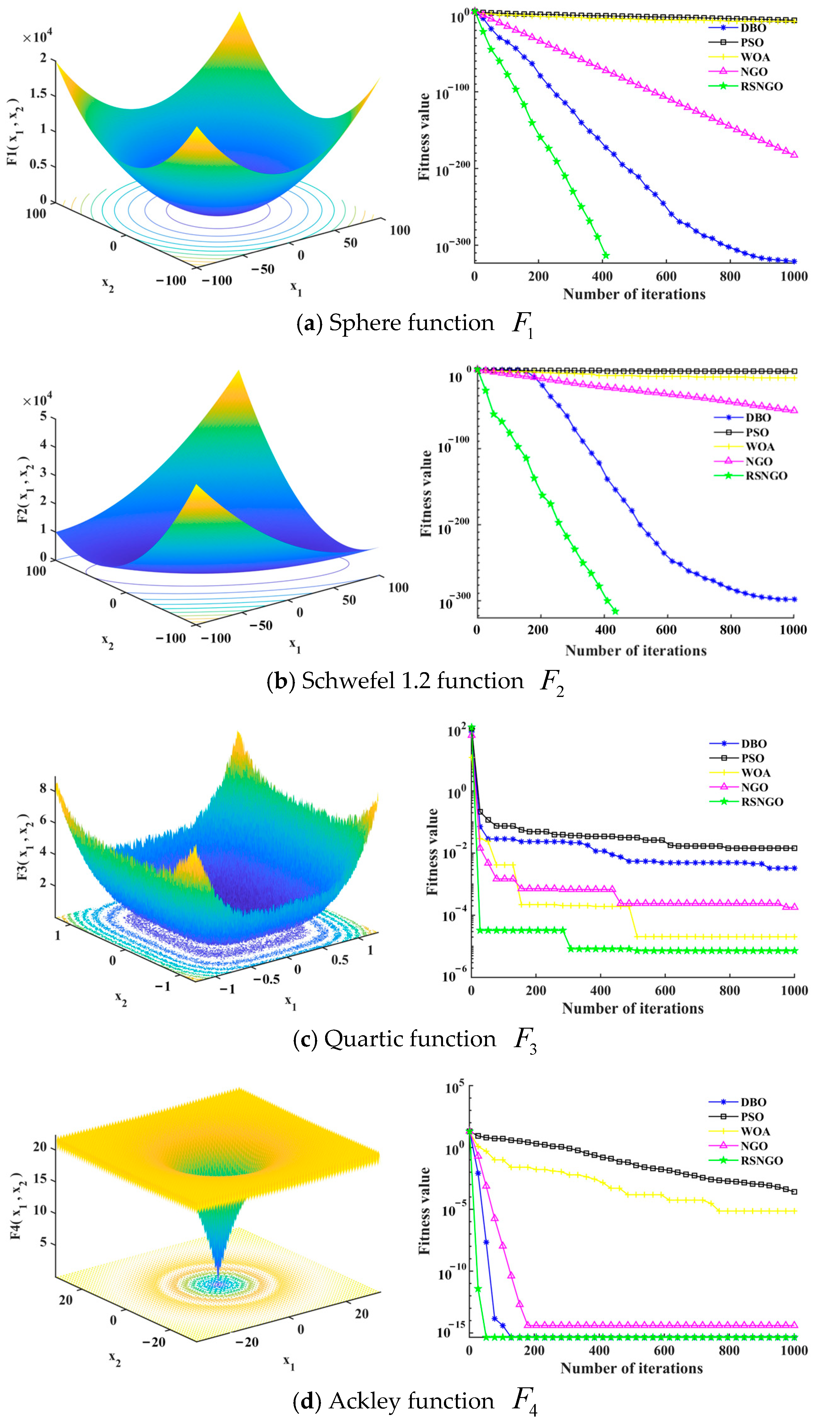
In order to verify the superiority of RSNGO, the performance of RSNGO algorithm is tested and analyzed, and the functions in the CEC function set [27] including $F_1$, $F_2$, $F_3$, and $F_4$ are selected for testing and validation, among which $F_1$, $F_2$, and $F_3$ are single-peak test functions, and $F_4$ is a multi-peak test function. The relevant properties of several functions are shown in

Table 1. Relevant properties of different functions.

Function Name	Formula	Search Area	Dimension
Sphere Function	$F_1(x)={\displaystyle \sum _{i=1}^N{x}_i^2}$	[−100, 100]	30
Schwefel 1.2	$F_2(x)={\displaystyle \sum _{i=1}^N({\displaystyle \sum _{j=1}^i{x}_j}}{)}^2$	[−100, 100]	30
Quartic Function	$F_3(x)={\displaystyle \sum _{i=1}^{N}i{x}_i^4}+random[0,1]$	[−1.28, 1.28]	30
Ackley’s Function	$\begin{array}{c}{F}_4(x)=-20\exp (-0.2\sqrt{{\displaystyle \frac{1}{N}}{\displaystyle \sum _{i=1}^N{x}_i^2}})\\ -\exp ({\displaystyle \frac{1}{N}}{\displaystyle \sum _{i=1}^N\cos 2\pi x_i})+20+e\end{array}$	[−32, 32]	30

. A comparative analysis is conducted with several common intelligent algorithms, including the unimproved NGO, PSO [28], WOA [29], and DBO [30]. The basic parameter settings of these intelligent algorithms are kept consistent. After 1000 optimization iterations, the convergence performance of different algorithms on F₁–F₄ benchmark functions was evaluated, and the corresponding convergence curves are presented in Figure 4.

As can be seen from the figure, RSNGO consistently outperforms the other compared algorithms in terms of both convergence speed and optimization accuracy. For unimodal functions, RSNGO converges to the optimal solution with significantly fewer iterations, indicating stronger local search capability and faster convergence speed. For multimodal functions, RSNGO not only maintains fast convergence but also achieves the lowest fitness values. These results demonstrate that RSNGO achieves a better balance between global exploration and local search, enabling it to effectively avoid local optima and achieve superior global optimization performance. Although benchmark functions can validate the optimization capability of metaheuristic algorithms, superior performance on such benchmarks does not necessarily imply better results in practical engineering optimization problems. Therefore, the effectiveness of RSNGO within the proposed bearing fault diagnosis framework is further verified through subsequent optimization-based diagnostic experiments.

3.2. Structural Design of a Multi-Fault Diagnosis Model

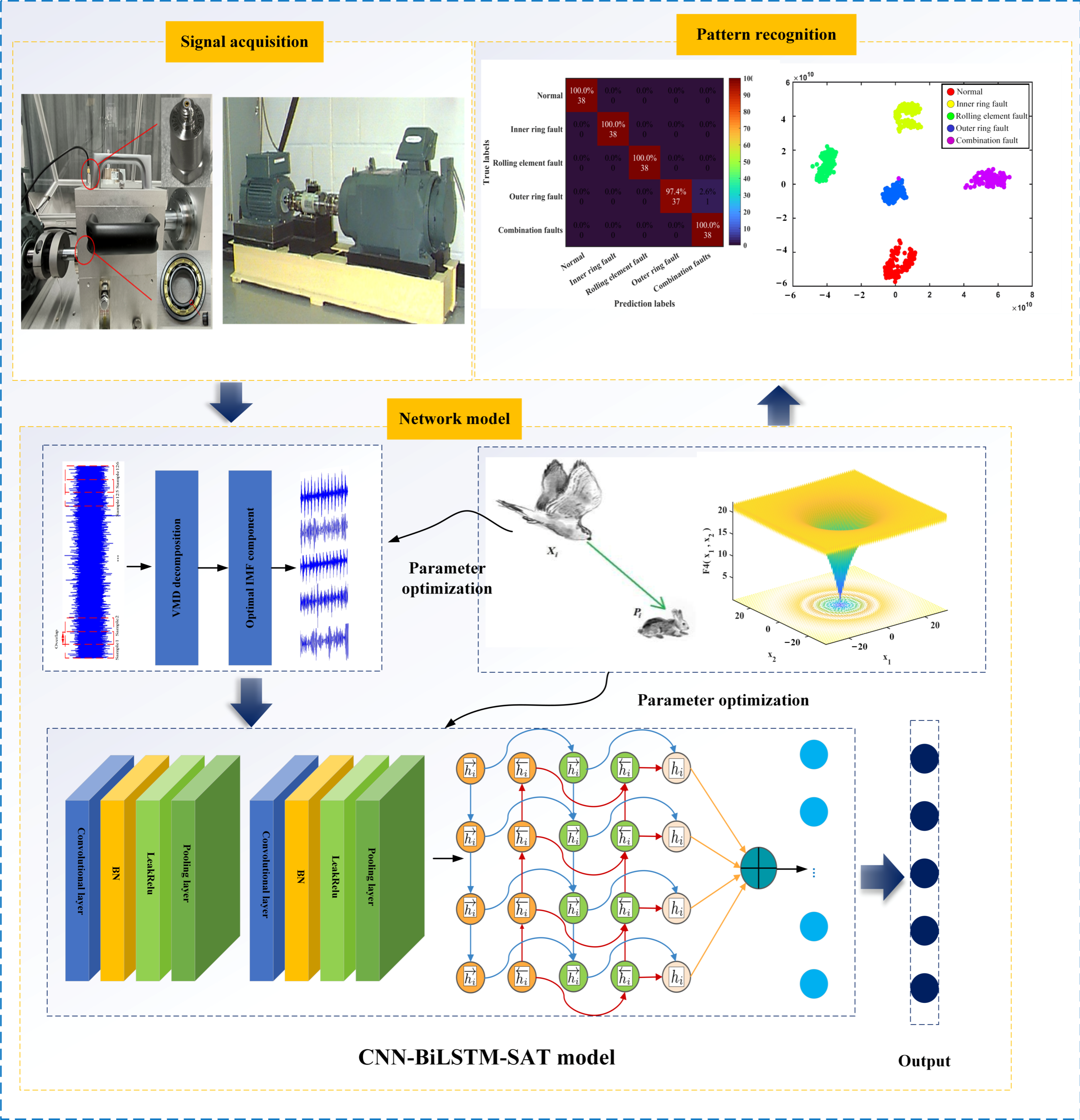
After the signal is decomposed using the RSNGO-VMD method, the optimal intrinsic mode function (IMF) component that contains the most prominent fault-related information is selected by adopting the minimum envelope entropy as the fitness function. Ten time-domain features are then extracted from this IMF to construct a sample set, which serves as the input to the fault diagnosis model. The proposed intelligent diagnosis framework mainly consists of a convolutional neural network (CNN), a bidirectional long short-term memory network (BiLSTM), and a self-attention mechanism (SAT). The key hyperparameters of the network are adaptively optimized by the RSNGO algorithm to enhance the model’s diagnostic performance and generalization capability. First, a two-layer CNN is employed to extract multiscale local features from the input data, effectively capturing representative time-domain fault patterns while reducing feature redundancy. The extracted high-level features are then fed into the BiLSTM network, which exploits bidirectional temporal dependencies to learn latent dynamic characteristics and long-range contextual information embedded in the fault signals. To further improve the representation of critical fault-related information, a self-attention mechanism is introduced after the BiLSTM layer. By assigning adaptive weights to different temporal features, the SAT module enables the network to focus on globally informative features and suppress irrelevant information, thereby enhancing the accuracy and robustness of fault feature extraction. Finally, the extracted discriminative features are mapped to different fault categories through a SoftMax classifier, achieving accurate identification of multiple fault conditions in cylindrical roller bearings. The overall architecture of the proposed diagnosis model is illustrated in Figure 5.

3.3. Model Diagnostic Process

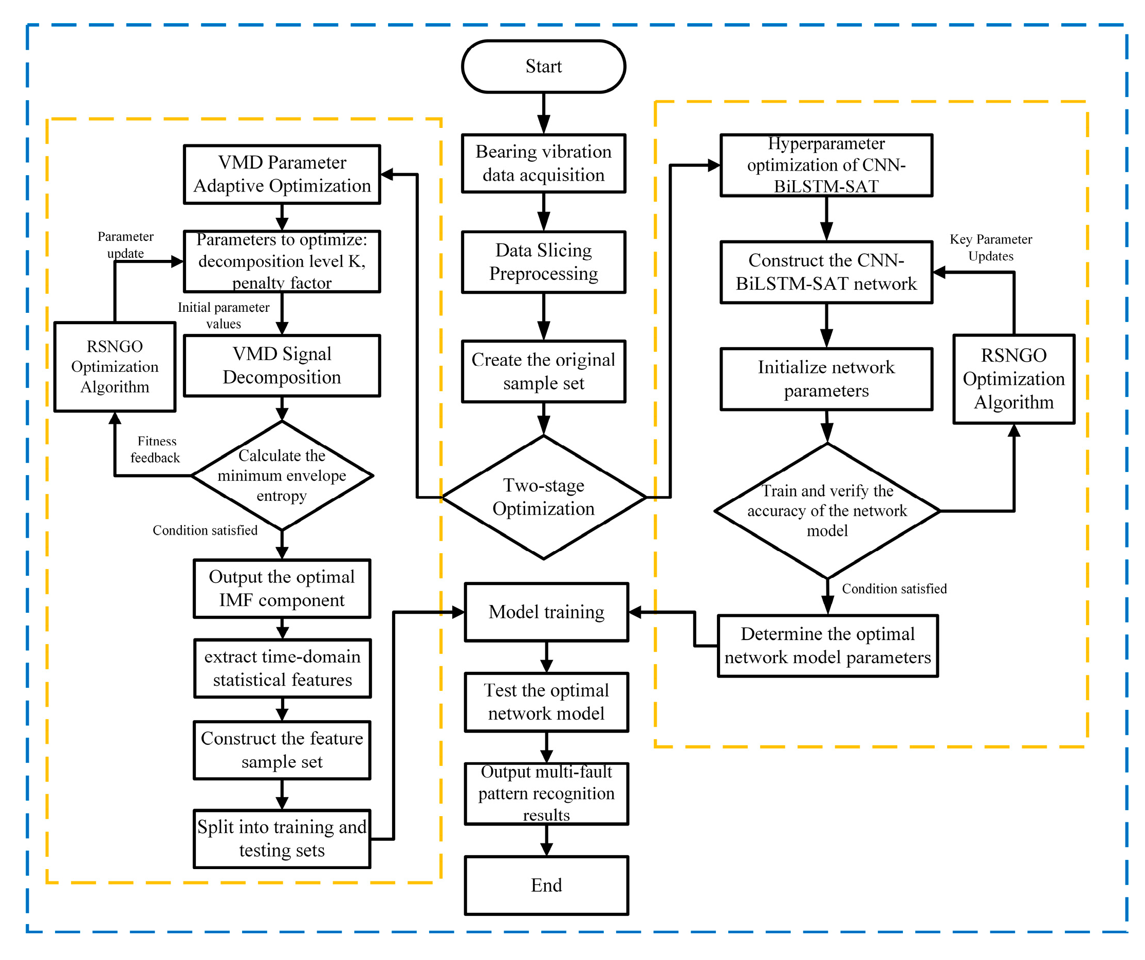
Aiming at the problem that cylindrical roller bearings are inaccurate in recognizing multi-fault features, this paper proposes a multi-fault pattern recognition model for bearings based on parameter optimization VMD and CNN-BiLSTM-SAT, and the recognition process is shown in Figure 6. The recognition process is specified as follows:

(1)

The collected bearing vibration signals were first preprocessed to construct the sample dataset. For raw signals under different health conditions, variational mode decomposition (VMD) was employed for signal decomposition. The RSNGO algorithm was utilized to adaptively optimize the VMD parameters, including the decomposition level K and the penalty factor α. The parameter search ranges, fitness function, and constraint conditions were kept consistent with those described in the previous section. Subsequently, the optimal intrinsic mode function (IMF) components were selected based on the minimum envelope entropy criterion, and ten time-domain statistical features were extracted to establish the feature sample set.

(2)

A CNN–BiLSTM–SAT network model was developed for bearing fault classification. The RSNGO algorithm was further employed to optimize key hyperparameters of the network, including the kernel size and the number of filters in the first CNN layer, the number of hidden neurons in the BiLSTM layer, and the initial learning rate. The network weights and biases were initialized, and corresponding parameter search ranges were defined. Classification accuracy was adopted as the fitness function for the optimization process. Through iterative training and parameter optimization, the optimal CNN–BiLSTM–SAT model was obtained.

(3)

The constructed sample dataset was divided into training and testing subsets. Based on the optimized model configuration, the training set was used for model learning, while the testing set was employed to evaluate the diagnostic performance. Finally, the identification results of multiple bearing fault modes were obtained and analyzed.

4. Experiment Design and Model Performance Analysis

4.1. Design of Experiments

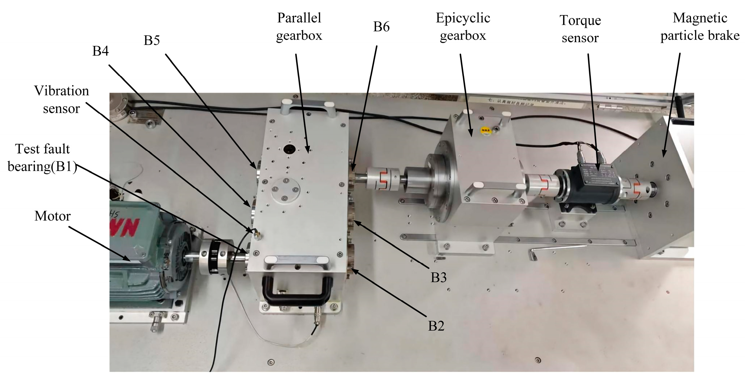
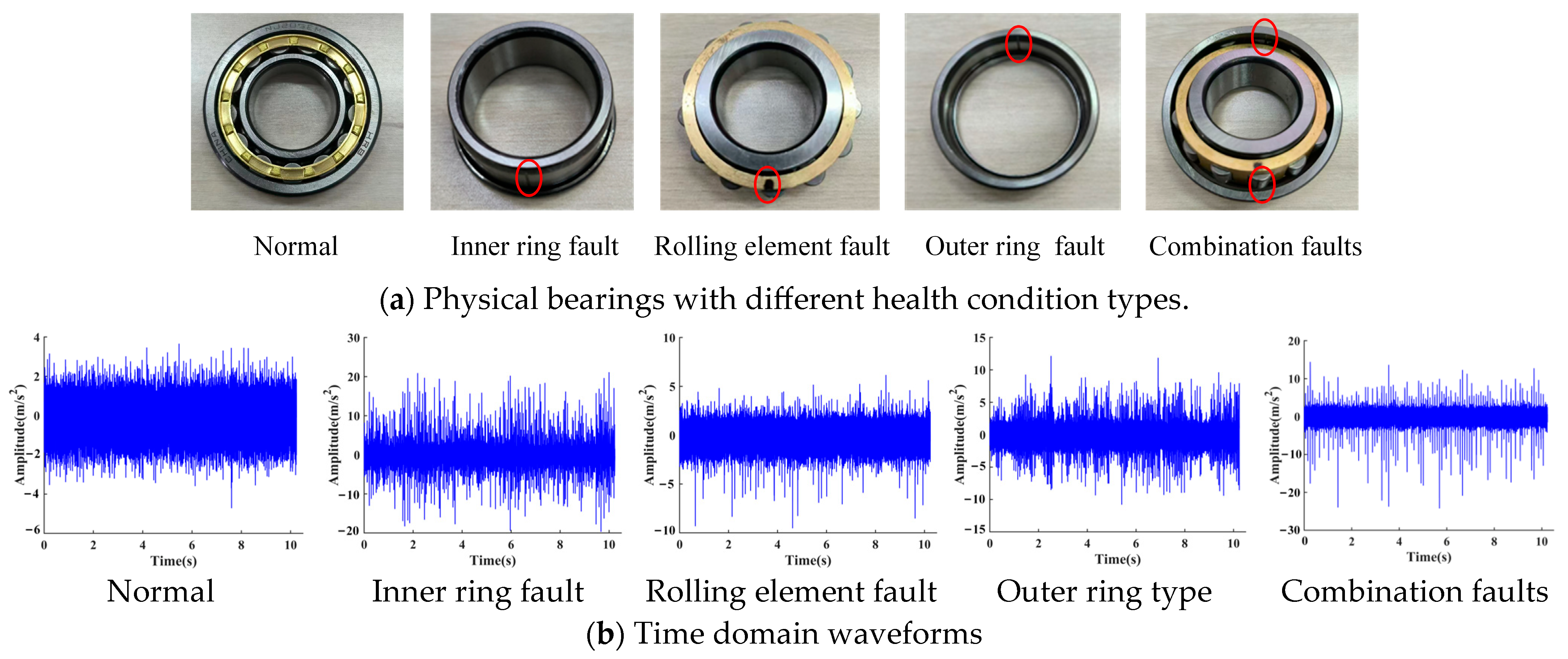
The bearing failure signals used in this paper are collected by the gearbox bearing fault test bench, which is shown in Figure 7. There are two types of bearings, including NJ205EM (inner ring separable) and NF205EM (outer ring separable), and the geometrical parameters of NF205EM and NJ205EM bearings are shown in

Table 2. Geometric parameters of NF205EM and NJ205EM.

Faulty Bearing Type	NF205EM	NJ205EM
Bearing outside diameter/mm	52	52
Bearing bore diameter/mm	25	25
Width/mm	15	15
Rolling element diameter/mm	7.49	7.49
Number of rolling elements	13	13
Contact angle β/(°)	0	0
Manufacturer	HRB	HRB
Bearing clearance	Normal radial internal	Normal radial internal clearance

. Artificial crack-like defects were introduced into the test bearings using electrical discharge machining (EDM). The resulting bearing health conditions comprised healthy, inner race fault, rolling element fault, outer race fault, and compound fault (simultaneous outer race and rolling element faults). For each defective bearing specimen, the defect had a uniform width of 0.5 mm and a depth of 0.4 mm. The four constant working conditions are simulated during the test, and the constant working speed and torque are 1010 r/min and 6 N·m, 1511 r/min and 11 N·m, 1812 r/min and 23 N·m, and 2115 r/min and 33 N·m, respectively. The gearbox contains six bearings, labeled B1–B6 in Figure 7. The diagnostic target is the bearing at position B1, which is mounted on the input shaft side. In each test, only this target bearing was replaced, while all other bearings remained in a healthy, undamaged condition. Vibration signals were measured using a vibration sensor installed directly above position B1. The sampling frequency was set to 12.8 kHz, and a uT3408M acquisition unit was employed to collect vibration signals from the test bearing under various health states. Each test lasted 10.24 s. For each operating condition, data were collected from a mix of two bearing types, NF205EM and NJ205EM. A total of five physical test bearings were used in the experiment.

Taking the analysis of the signals collected at a rotational speed of 1511 r/min and a torque of 11 N·m as an example, Figure 8 shows the time-domain waveforms corresponding to different bearing health conditions. Owing to the pronounced amplitude differences among vibration signals under different fault states, adopting a uniform ordinate scale would compress the local impulsive features in low-amplitude signals. Therefore, to preserve the observability of the original waveform characteristics of each state, independent amplitude scales are used for display.

4.2. Data Processing and Dataset Construction

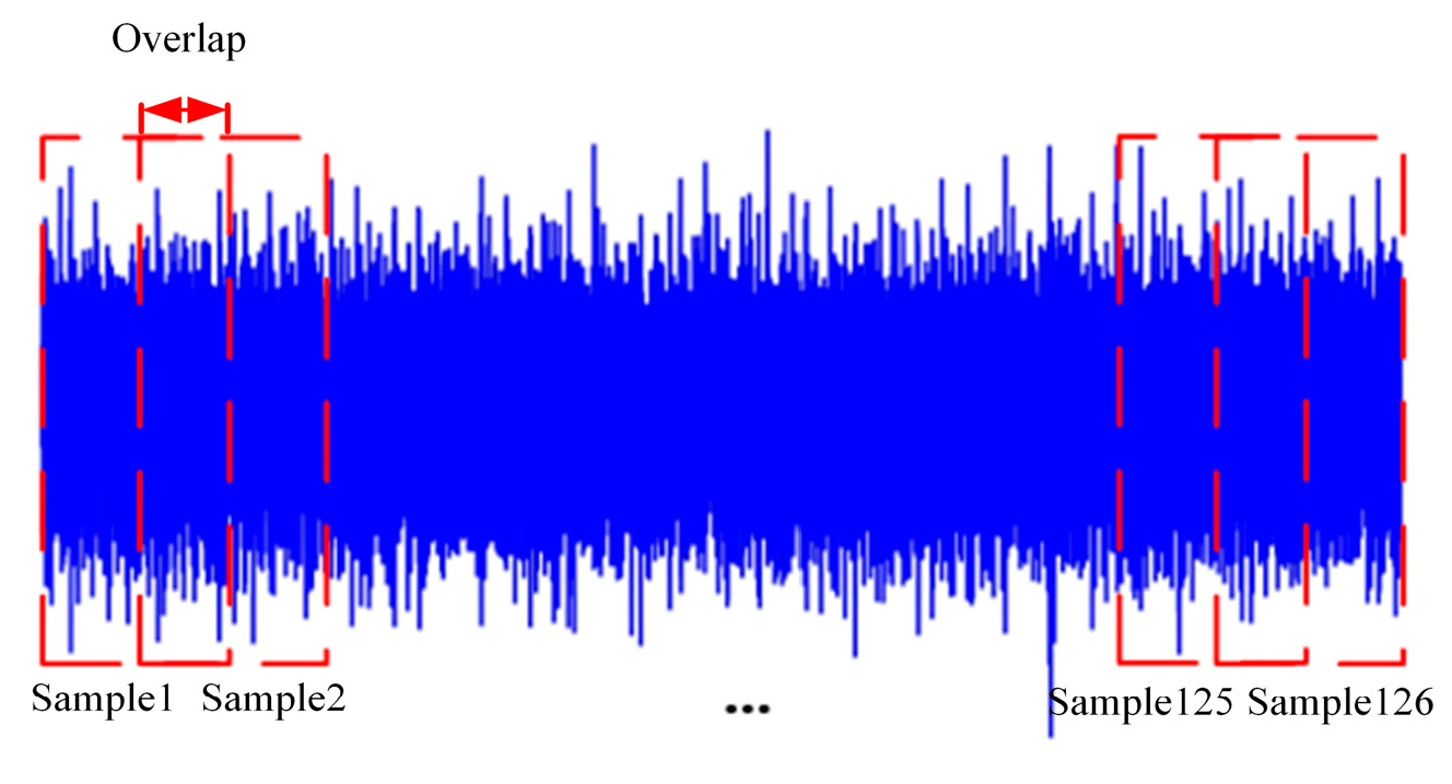
The acquired bearing vibration signals are one-dimensional time-series signals, and the fault information is predominantly concentrated in the impulsive signals generated under different operating conditions. Therefore, the overlapping sampling [31] data augmentation method is employed to slice and preprocess the vibration signals collected in the above tests; the overlapping segmentation strategy serves only to produce a sufficient number of independent signal segments for feature extraction. The slice preprocessing procedure is illustrated in Figure 9. For the one-dimensional vibration signals of different state types, the maximum sample size $M^{\prime }$ that can be processed is

$$M^{\prime }=\left[{\displaystyle \frac{L_n-\overline{N}}{\overline{N}\cdot \mu }}\right]$$

(24)

where $L_n$ is the one-dimensional vibration signal length, $\overline{N}$ is the sampling fixed window length, $\mu$ is the overlap rate, and $\left[\cdot \cdot \cdot \right]$ is the sample size rounded down.

Taking the vibration signals acquired under five bearing health conditions at a rotational speed of 1511 r/min and a load torque of 11 N·m as an example, a fixed-length sliding window was employed to segment the continuous vibration data to fully exploit the useful information contained in the collected signals. The window length was set to 2048 points and the sliding step to 1024 points, yielding a 50% overlap between adjacent samples. After the sliding window processing, 126 initial samples were obtained for each bearing health condition, and all samples were labeled according to their corresponding health states, as detailed in

Table 3. Sample division and labeling.

Label	Bearing Health Condition	Rotate Speed/(r/min)	Torque/(N·m)	Fault Degree/(Width × Depth/mm)	Number of Samples Under Different Bearing Conditions
1	Normal	1511	11	—	126
2	Inner ring fault	1511	11	0.5 × 0.4	126
3	Rolling element fault	1511	11	0.5 × 0.4	126
4	Outer ring fault	1511	11	0.5 × 0.4	126
5	Combination faults	1511	11	0.5 × 0.4	126

. It should be noted that the sliding window operation was only used to increase the sample quantity and improve feature coverage. These segmented signals are subsequently processed independently using the RSNGO-VMD algorithm, where each segment is transformed into an independent feature vector. Accordingly, dataset partitioning is performed at the feature vector level thereafter.

After segmentation and preprocessing of the collected vibration signals, the RSNGO algorithm was employed to optimize the key parameters of variational mode decomposition (VMD), the number of decomposition modes $K$, and the penalty factor $\alpha$, aiming to extract fault-related features more comprehensively under different bearing health states. Following the approach in [32], the RSNGO parameters were determined through extensive tuning experiments: the population size was set to 30, the maximum number of iterations was set to 20, the penalty factor $\alpha$ of VMD was searched within the range [100, 2500], and the number of modes $K$ was searched within the range [3, 10]. The minimum envelope entropy was adopted as the fitness function—a lower value indicates more pronounced fault information. After 20 optimization iterations, the optimal parameter combinations corresponding to the five bearing health states were obtained, as detailed in

Table 4. Optimization results of bearing data under different state types.

Bearing Health Condition	Selected IMF Index	Decomposition Levels/K	Penalty Factor/α	Minimum Envelope Entropy
Normal	3	5	1433	7.29
Inner ring fault	4	10	137	7.18
Rolling element fault	2	4	655	7.32
Outer ring fault	10	10	899	7.23
Combination faults	5	10	2500	7.3

“Selected IMF Index” denotes the ordinal number of the IMF with the minimum envelope entropy among the K decomposed modes.

.

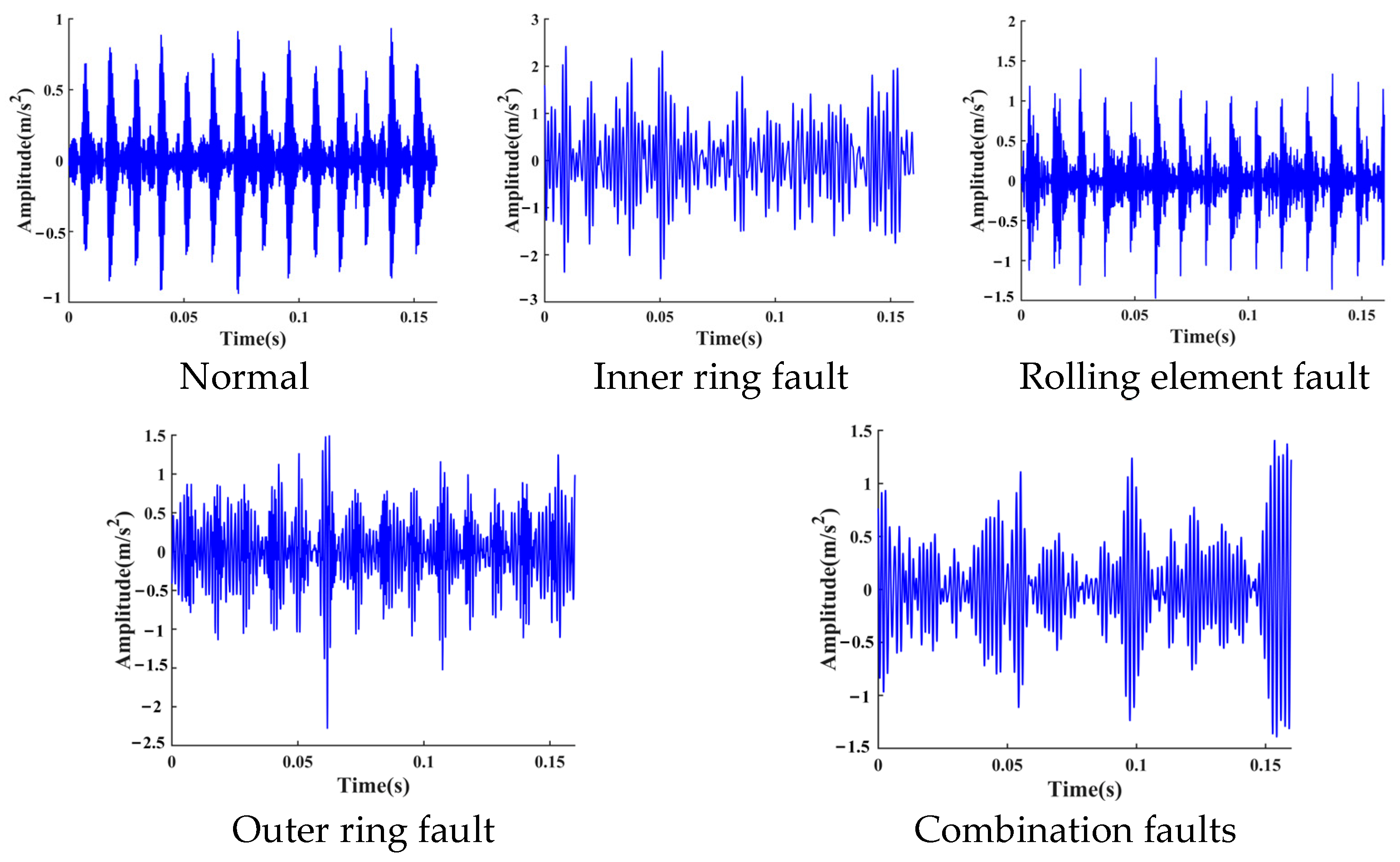
Based on the optimized parameters, VMD was applied to decompose each sample obtained from the preceding data segmentation step, and the optimal intrinsic mode function (IMF) component was selected according to predefined criteria. Figure 10 shows the time-domain waveforms of the selected optimal IMF components under five bearing health conditions. To demonstrate the effect of RSNGO-VMD on data processing, a short time window is selected in this paper to highlight the local impulsive behavior. Compared with the original vibration signal, the signal processed by the RSNGO-VMD method exhibits significantly reduced amplitude fluctuations and more distinct periodic impulse components. This indicates that RSNGO automatically determines the optimal decomposition parameters of VMD by minimizing the envelope entropy, and the optimized parameters enable the extracted IMF components to contain more fault-related information while reducing redundant interference components. Therefore, the superior convergence capability of RSNGO demonstrated in Section 3 is directly reflected in the quality of vibration feature representation. Subsequently, ten time-domain feature metrics are extracted from the obtained optimal IMF components, thereby transforming the previously sliced data samples into independent feature vectors. The resulting feature vector sample set is then split into training and test sets at a ratio of 7:3 to serve as the input for the subsequent network model. This partitioning is performed after the completion of feature construction, ensuring that both model training and evaluation are conducted on independent feature samples.

4.3. Optimal Model Parameter Configuration

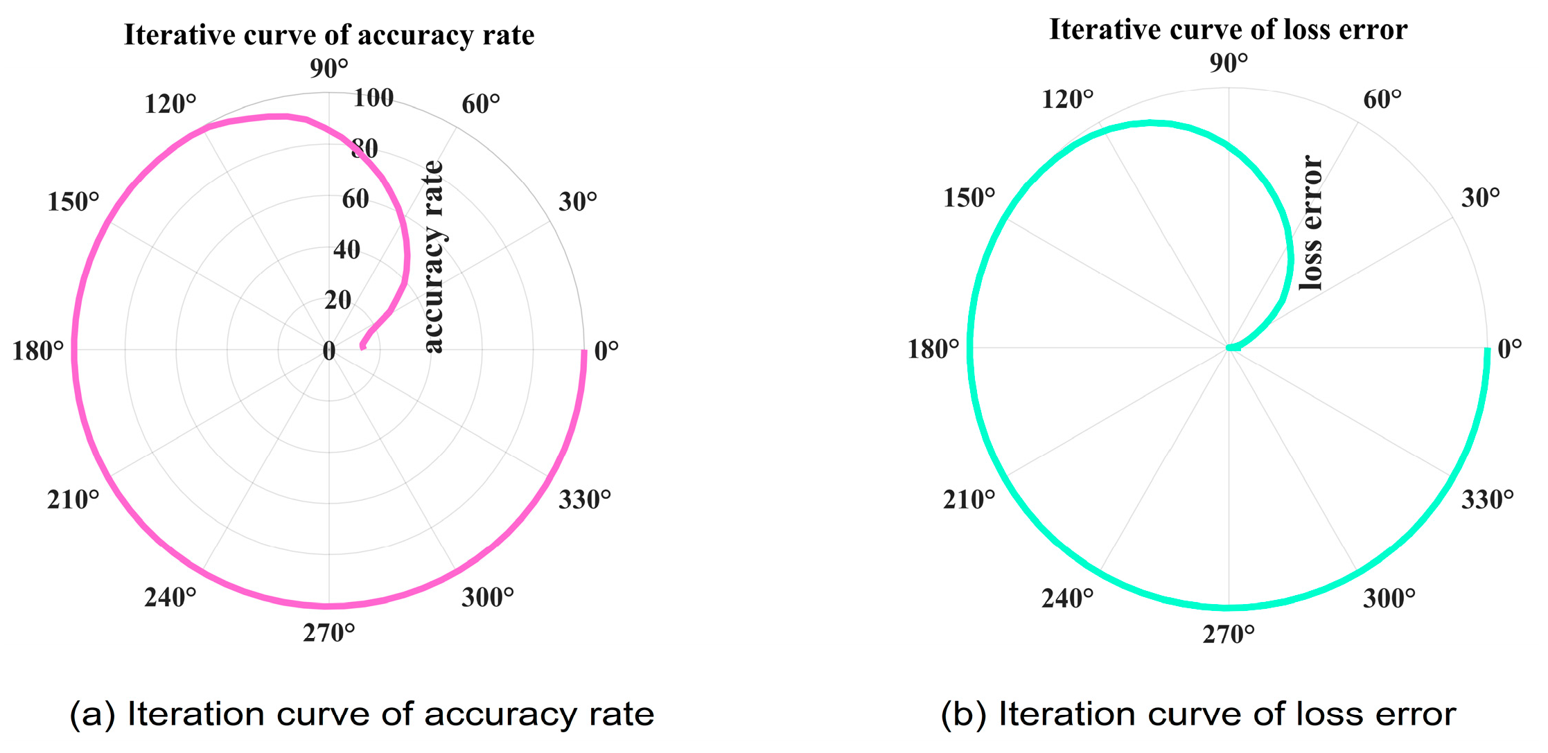
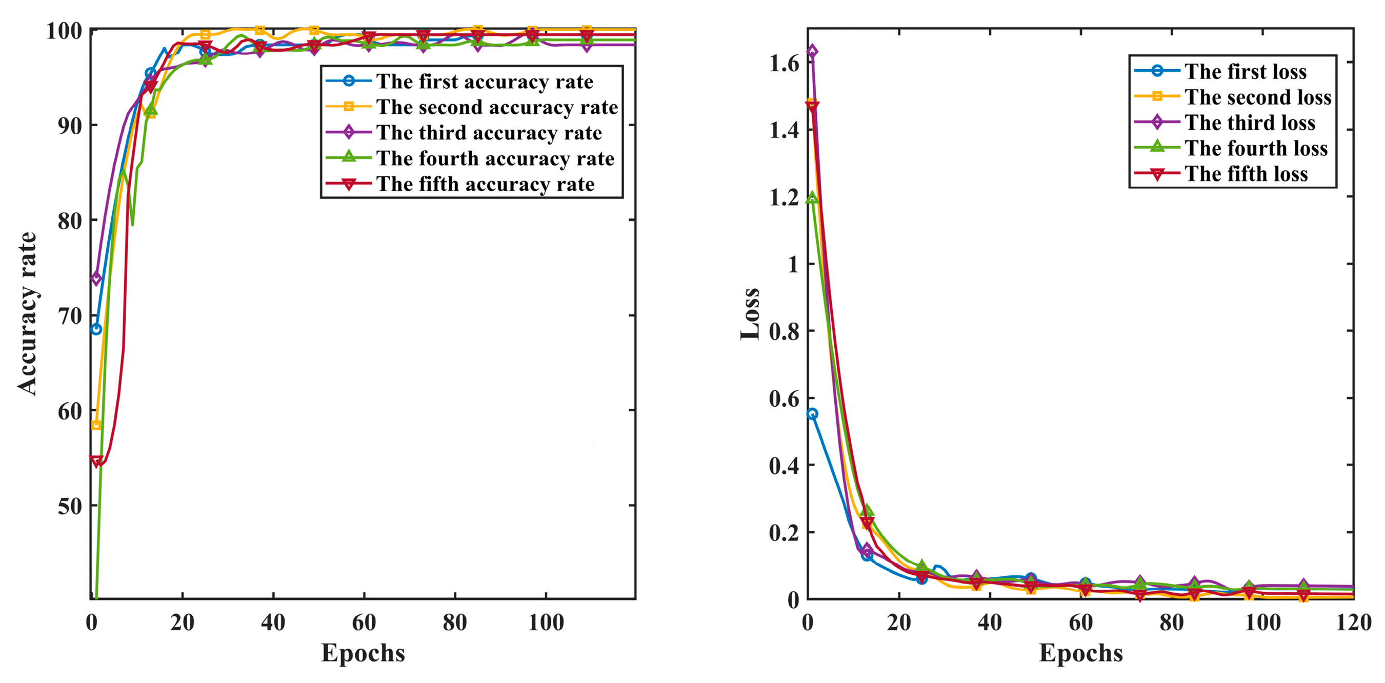
To determine the optimal network configuration of the proposed method, the RSNGO algorithm was employed to optimize several key hyperparameters of the model, including the kernel size of the first CNN layer, the number of convolution kernels, the initial learning rate, and the number of hidden neurons in the BiLSTM layer. Classification accuracy was selected as the fitness function. The search ranges of these parameters were set to [2, 8], [5, 20], [0.001, 0.01], and [20, 50], respectively. After 10 optimization runs, the model achieved the highest classification accuracy, which became stable after approximately one-third of the total iterations, while the loss value gradually converged to its minimum. The training accuracy and loss curves are presented in Figure 11. As illustrated in Figure 11, the classification accuracy increases rapidly during the early stages of training and gradually stabilizes at a high level. Meanwhile, the loss value continuously decreases and eventually approaches zero. These results demonstrate the effectiveness of the proposed model in feature learning and parameter optimization, as well as its excellent convergence stability and training robustness. The optimal configuration obtained by the RSNGO algorithm consists of a kernel size of 6 for the first CNN layer, 16 convolution kernels, an initial learning rate of 0.008, and 32 hidden neurons in the BiLSTM layer.

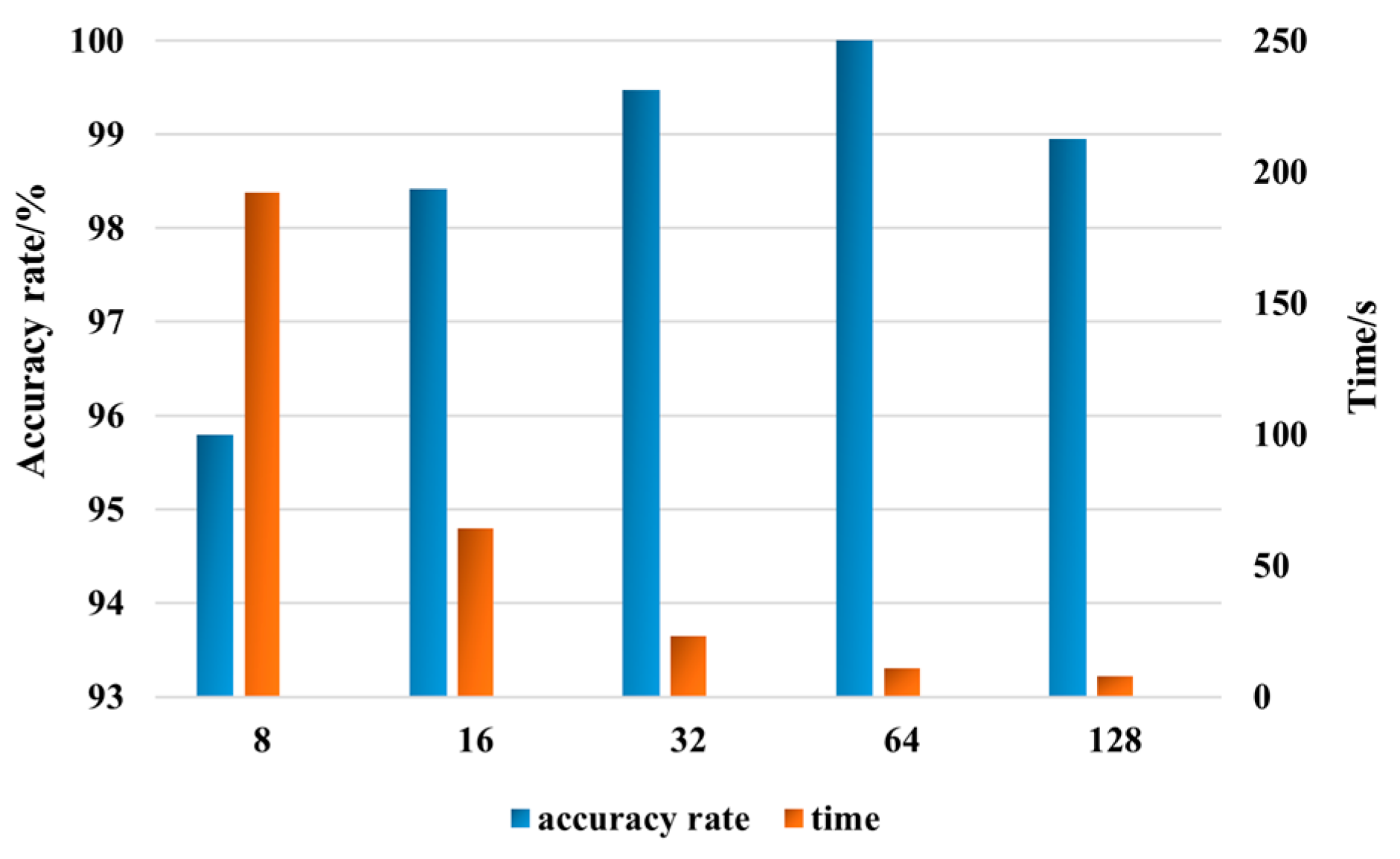
During model training, the batch size refers to the number of samples fed into the network in a single iteration to compute gradients and update parameters, and it has a significant impact on network performance. A small batch size prolongs training time and, owing to the high variance of gradient estimates, tends to cause unstable parameter updates, thereby reducing classification accuracy. Conversely, while an excessively large batch size improves computational efficiency, it increases memory consumption and may cause the model to converge to sharp minima, impairing generalization ability. To determine the optimal batch size, we evaluated the effect of different batch sizes on classification accuracy and training time, and the results are shown in Figure 12.

The results presented above indicate that increasing the batch size generally reduces training time and improves the stability of gradient updates. However, an excessively large batch size may limit the model’s generalization ability. After considering both classification accuracy and computational efficiency, the batch size was ultimately set to 64. This parameter setting consistently demonstrated superior performance in the parameter selection experiments and achieved an ideal balance among convergence stability, computational cost, and diagnostic accuracy. Meanwhile, the kernel size and number of kernels in the second CNN layer were set to 2 and 8, respectively. The self-attention module employed a single attention head with 50 key channels and 50 value channels. Based on extensive comparative experiments, the number of training epochs was set to 120, and the Leaky ReLU function was adopted as the activation function. The cross-entropy loss function (CrossEntropyLoss) was utilized as the optimization objective, and the Adaptive Moment Estimation (Adam) algorithm was employed to optimize the network parameters. In addition, Dropout layers were introduced after the pooling and fully connected layers to mitigate overfitting. The optimal hyperparameter configuration of the proposed network model is summarized in

Table 5. Main parameters of the optimal network model.

Parameter	Value	Parameter	Value
1CNN__kernel_size	6	Learning rate	0.008
1CNN__kernel_number	16	Epoch	120
2CNN__kernel_size	2	Batch size	64
2CNN__kernel_number	8	Loss function	Cross Entropy Loss
BiLSTM_hidden_size	32	Activation function	Leaky ReLU
SAT_head	1	Optimizer	Adam
SAT_key	50	SAT_value_channel	50

.

4.4. Analysis of Model Diagnosis Results

After the network parameters were determined, the feature vector dataset was fed into the proposed model for five independent runs. The diagnostic accuracies obtained in the five tests were 99.47%, 100.00%, 98.42%, 98.95%, and 99.47%, respectively, yielding an average accuracy of 99.26%. The diagnostic results of the five tests are presented in Figure 13.

As shown in the training process, both the accuracy and loss curves gradually converged after approximately 40 epochs. At this stage, the accuracy remained above 97.89%, while the loss value continuously decreased and approached zero, indicating that the proposed model possesses excellent feature learning capability and convergence performance. Moreover, the accuracy and loss curves obtained from the five independent tests exhibited highly consistent trends, demonstrating the robustness and stability of the proposed method. These results indicate that the superior diagnostic performance is attributable not only to the integration of SAT into the CNN-BiLSTM framework but also to the parameter optimization capability of RSNGO. The VMD optimized by RSNGO provides more informative fault-related features, while the RSNGO-based parameter optimization enables the network model to acquire more appropriate learning configurations, thereby allowing the network to achieve enhanced feature representation and classification performance.

4.5. Comparison of Model Experiment Analysis

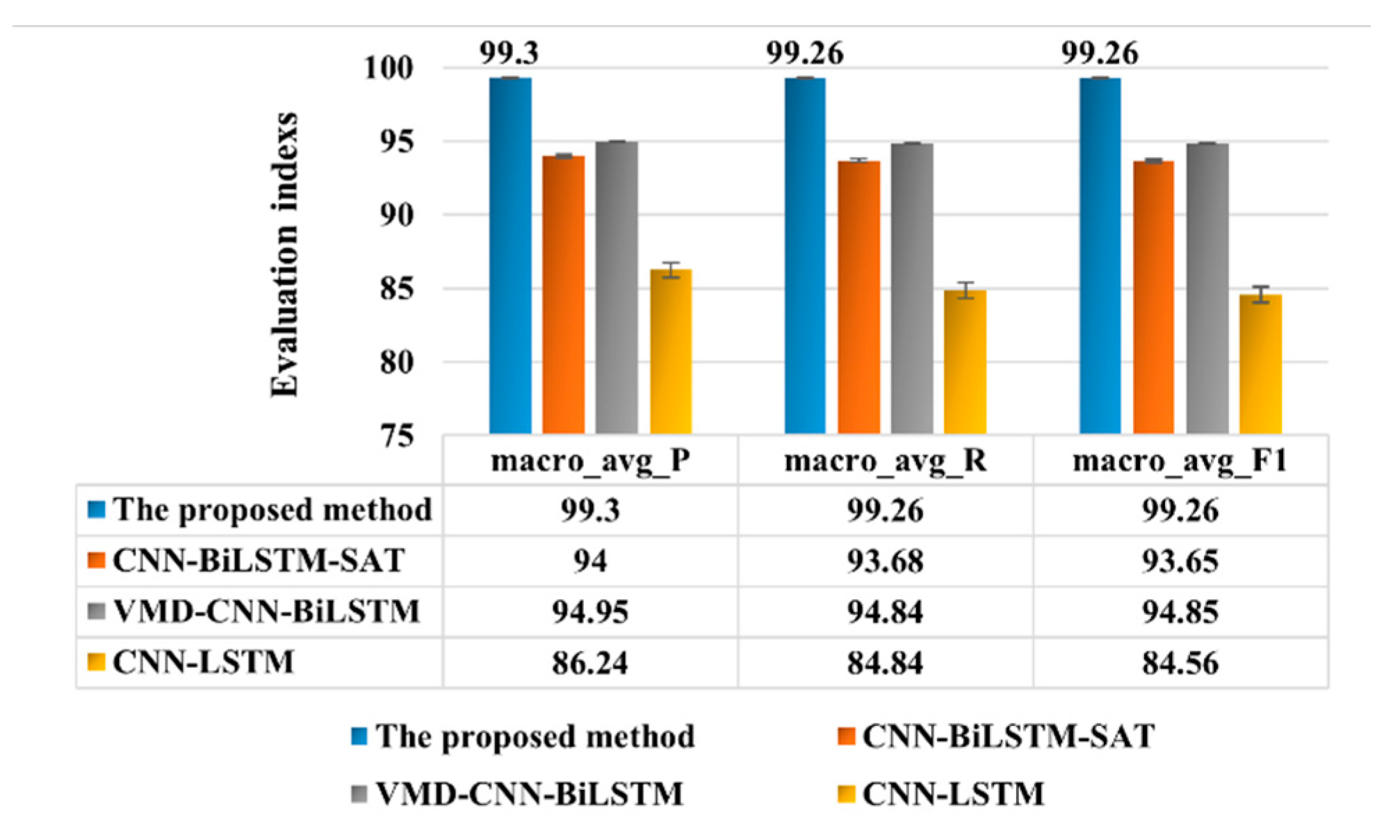
To validate the effectiveness and superiority of the proposed method, we conduct a comparative analysis with CNN-LSTM, CNN-BiLSTM-SAT, and the conventional VMD-CNN-BiLSTM model without parameter optimization. For fair comparison, all baseline models are reasonably tuned according to their network characteristics, primarily including the learning rate, batch size, number of hidden units, and dropout rate. These parameters are determined based on preliminary experimental results and common settings adopted in related studies. Precision, recall, and F1-score are employed as evaluation metrics to measure the classification performance of each model. To ensure the reliability of the experimental results and eliminate the influence of randomness, five independent tests were conducted for each model, and the macro-average performance metrics were calculated. The results are illustrated in Figure 14.

It can be observed that all performance indicators of the proposed model exceeded 99%. Under the same experimental settings and after individual parameter adjustment of each model, the proposed method achieved improvements of 4.35%, 4.42%, and 4.41% in macro-average precision, recall, and F1-score compared with the conventional VMD-CNN-BiLSTM model. This improvement can be attributed to the joint contribution of the optimized VMD preprocessing and the SAT-enhanced feature extraction architecture. RSNGO provides adaptive parameter selection for signal decomposition, while SAT further improves the discriminative capability of deep feature representation. Moreover, compared with the CNN-BiLSTM-SAT and CNN-LSTM models, the proposed method improved macro-average precision by 5.30% and 13.06%, recall by 5.58% and 14.42%, and F1-score by 5.61% and 14.70%, respectively. The results demonstrate that the RSNGO-optimized VMD preprocessing effectively reduces noise and redundant information in the raw signals, providing higher-quality input features for subsequent network learning. The proposed model exhibits excellent classification performance and robustness, fully highlighting its effectiveness and practical application potential in the field of multi-fault diagnosis of cylindrical roller bearings.

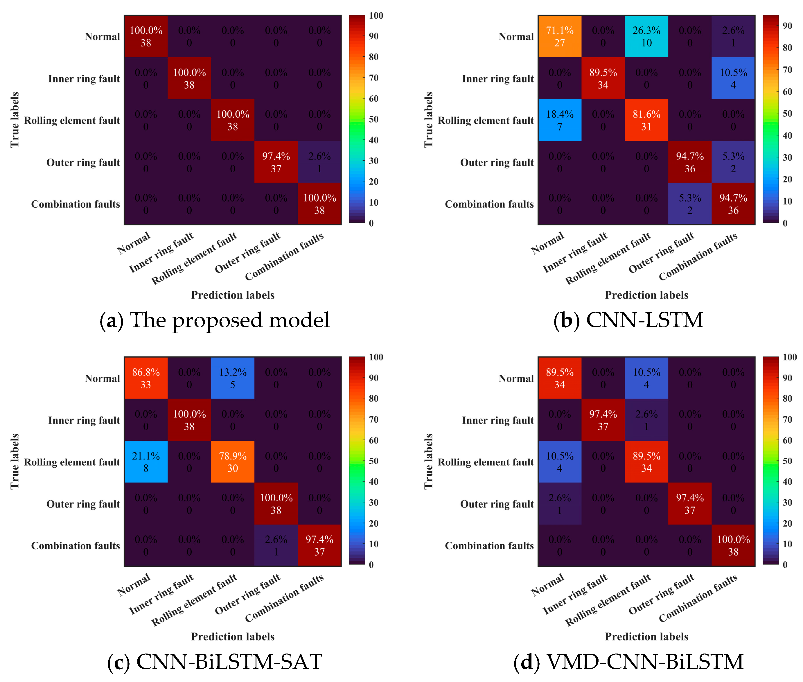
Meanwhile, the confusion matrix (CM) [33] was employed to further evaluate the classification performance of different models. Taking the first test result as an example, the confusion matrices of the different models are shown in Figure 15. CNN-LSTM, CNN-BiLSTM-SAT, and the unoptimized VMD-CNN-BiLSTM model all exhibited misclassifications to varying degrees, particularly between the normal state and rolling element fault, as well as between the outer race fault and compound fault, where noticeable confusion was observed. These results indicate that their capability to identify complex fault patterns remains limited. In contrast, the proposed model demonstrated the best discriminative performance across all five operating conditions: the samples corresponding to the normal state, inner race fault, rolling element fault, and compound fault were all classified with 100% accuracy, and only one outer race fault sample was incorrectly identified as a compound fault. These results demonstrate that the proposed model can effectively extract discriminative features across different fault categories while preserving strong class separability. This further indicates that the optimization capability of RSNGO is effectively transferred to the feature learning stage, rather than being limited to the numerical convergence advantage of the optimization algorithm itself.

4.6. Model Diagnosis Results Under Different Optimization Algorithms

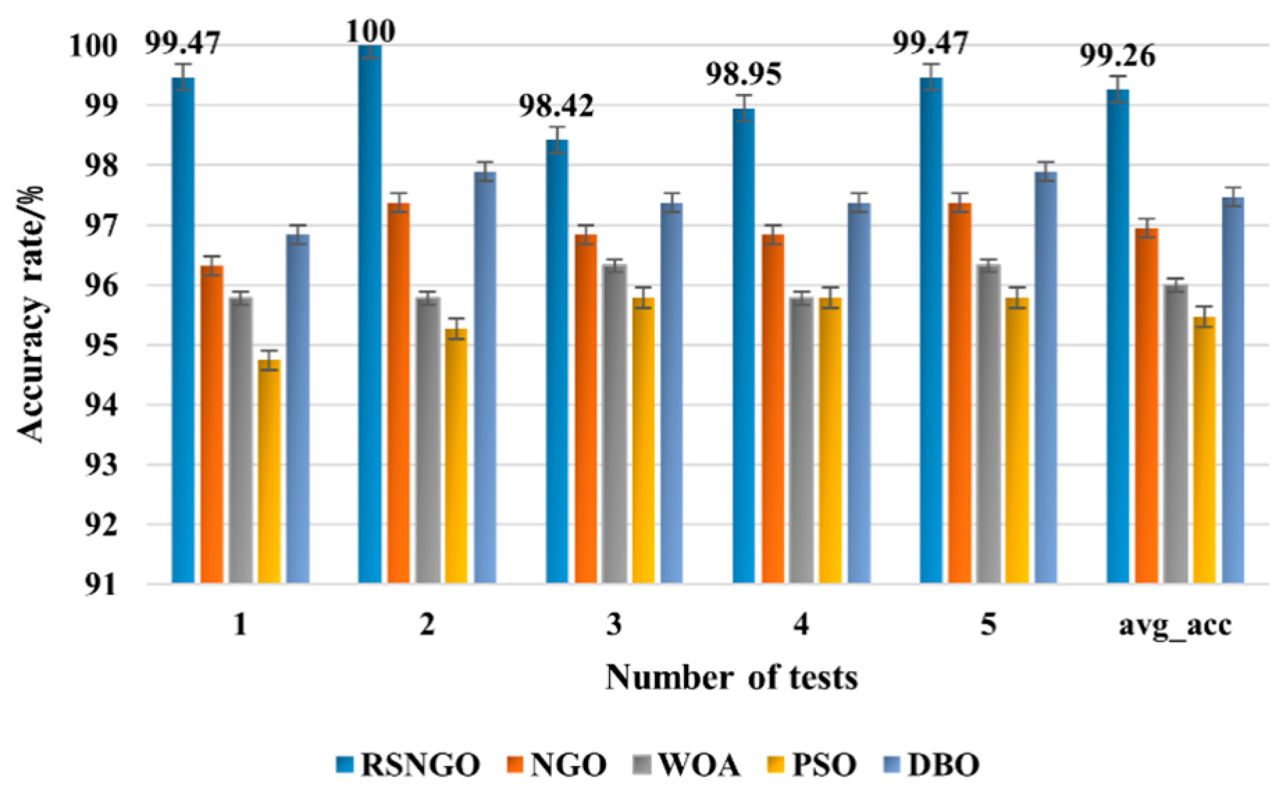
To validate the effectiveness of the proposed RSNGO algorithm in optimizing deep network parameters, this study selects several representative metaheuristic optimization algorithms—namely NGO, WOA, PSO, and DBO—as comparative methods. Since all these algorithms are based on swarm intelligence for parameter optimization and share the same optimization objective and search mechanism as RSNGO, they enable an objective assessment of performance differences among various intelligent optimization algorithms in model parameter tuning. Each optimization algorithm is employed to fine-tune the key network parameters, and both the training and testing procedures are repeated five times. The final recognition results are presented in Figure 16. The results demonstrate that the model optimized by RSNGO achieves the highest recognition accuracy, outperforming NGO, WOA, PSO, and DBO by 2.31%, 3.26%, 3.79%, and 1.79%, respectively. These findings indicate that the superior search capability of RSNGO is not only manifested during the optimization process but also effectively enhances the network model’s ability to extract and recognize complex fault features.

4.7. Ablation Analysis of Optimization Strategies

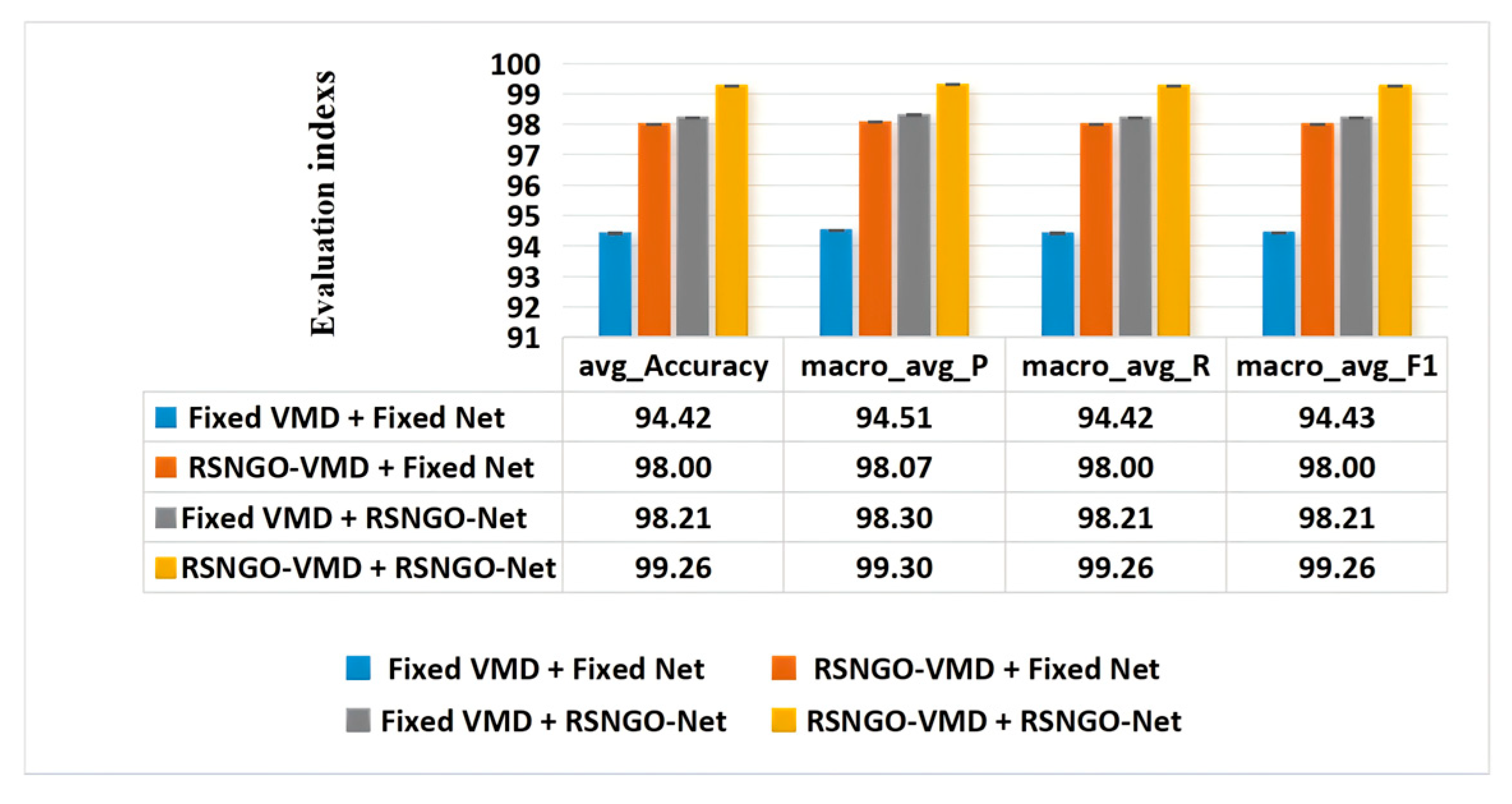
To thoroughly investigate the contribution of each optimization component in the proposed model framework, ablation experiments were conducted. As the method involves two optimization stages—namely, RSNGO-based VMD parameter optimization and RSNGO-based network hyperparameter optimization—four distinct configuration schemes were designed, as presented in

Table 6. Ablation model design.

Model	VMD Parameter Optimization	Network Parameter Optimization
M1	Fixed VMD	Fixed CNN-BiLSTM-SAT
M2	RSNGO-VMD	Fixed CNN-BiLSTM-SAT
M3	Fixed VMD	RSNGO-CNN-BiLSTM-SAT
M4	RSNGO-VMD	RSNGO-CNN-BiLSTM-SAT

.

Each configuration was tested five times consecutively under identical experimental conditions, and the macro-averaged performance metrics across different models were calculated. The parameters of the unoptimized framework were determined based on preliminary experimental results and settings commonly adopted in related studies. The results are presented in Figure 17.

As shown in the figure, the baseline model (with fixed VMD parameters and manually set network parameters) achieves an accuracy of 94.42%. The introduction of RSNGO-optimized VMD raises the accuracy to 98.00% (+3.58%), while fixed VMD combined with RSNGO-based network optimization yields 98.21% (+3.79%). The complete model integrating both optimization strategies attains the best performance, with accuracy and macro F1-score both reaching 99.26%, surpassing the model optimized only on VMD and the model optimized only on the network by 1.26% and 1.05%, respectively. These results indicate that the two strategies are complementary: RSNGO-VMD improves signal decomposition quality and the separability of fault-related features, whereas RSNGO-Net enhances the feature learning capability of CNN-BiLSTM-SAT. The superior performance of the proposed method stems from the synergistic optimization of signal decomposition and network architecture, validating the effectiveness of each component of the framework.

4.8. Robustness Test of the Model

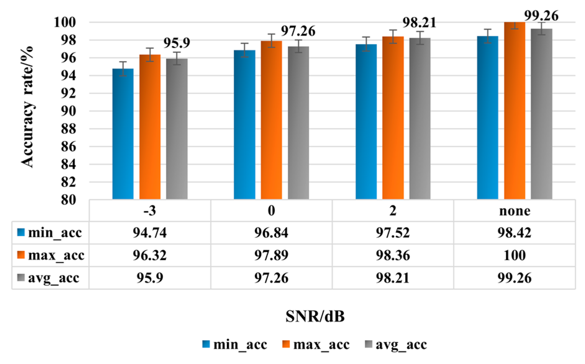
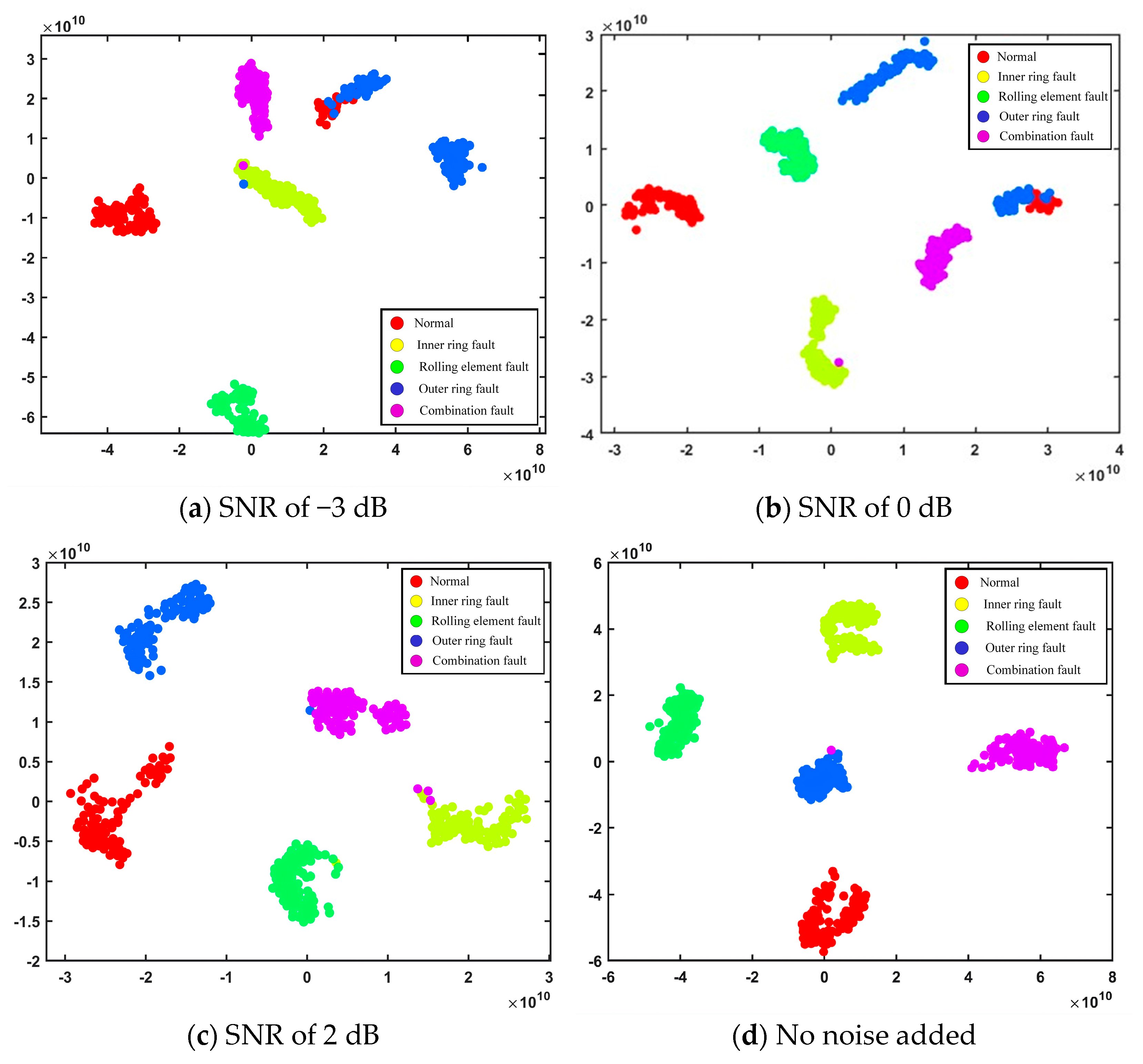
To further validate the effectiveness of the proposed model and analyze its robustness, Gaussian white noise with different signal-to-noise ratios are added to the measured signals to simulate the interference in different noise environments, respectively. Five times training and testing are conducted for each noise-added signal, and the accuracy rate of the test set is shown in Figure 18. Meanwhile, the t-Distributed Stochastic Neighbor Embedding (t-SNE) [34] algorithm is used to visualize and analyze the test results of different noise-added signals. t-SNE figures with five colors represent five different health state labels. The t-SNE algorithm can effectively transform the data points from the high-dimensional space to the low-dimensional space while maintaining the local and global structural features of the original data as much as possible. t-SNE visualization is shown in Figure 19, taking the first test result as an example.

As shown in Figure 18 and Figure 19, the classification accuracy on the test set gradually improves with increasing signal-to-noise ratio (SNR). Under various noise interference conditions, the proposed model achieves an average classification accuracy of 97.12%; meanwhile, the clustering patterns of the five state labels become increasingly distinct, and clear decision boundaries are formed among different fault categories. When the SNR drops to −3 dB, the optimized decomposition parameters obtained via RSNGO enable VMD to suppress irrelevant interferences while retaining more fault-related components. As a result, the classification performance does not degrade significantly, and the average accuracy remains at 95.90%. The corresponding t-SNE visualization results indicate that the outer race fault samples partially overlap with the healthy bearing samples, whereas the remaining categories remain well-clustered and clearly separable. These results demonstrate that the proposed model possesses excellent anti-noise capability and can effectively distinguish different fault types of cylindrical roller bearings under noisy operating conditions.

4.9. Adaptability Verification of the Diagnostic Model

In order to comprehensively assess the generalization ability of the proposed model, the self-acquired data from the test bench under other operating conditions and the CWRU bearing fault dataset are used for validation analysis, respectively.

(1)

Self-acquired test analysis under other operating conditions

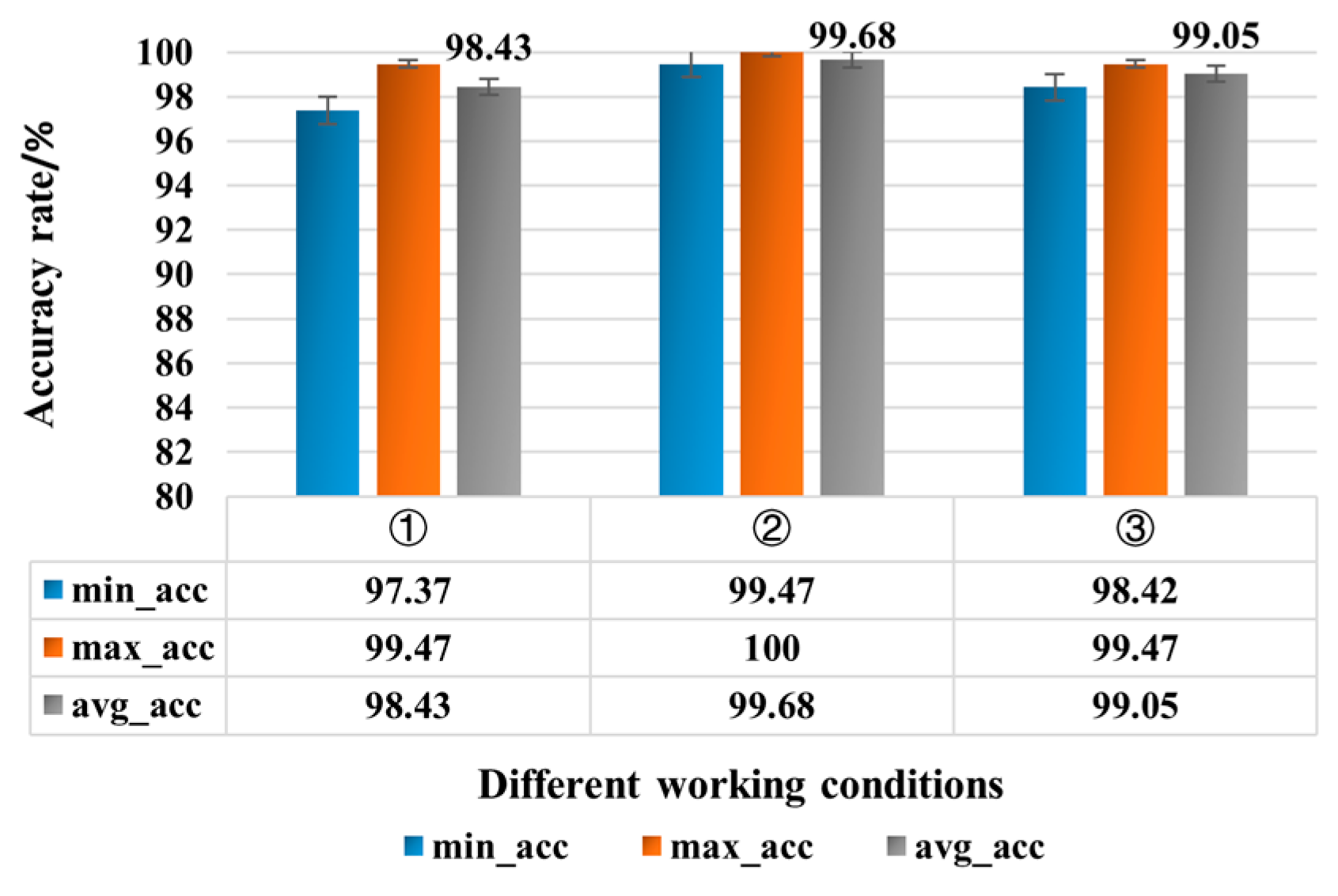
The proposed test bench is also used to simulate the other three conditions: ① the measured speed of 1010 r/min and torque of 6 N·m; ② the measured speed of 1812 r/min and torque of 23 N·m; ③ the measured speed of 2115 r/min and torque of 33 N·m, and the sampling parameters are the same as the test parameters of this paper. The bearing state samples are preprocessed under different working conditions and the proposed network model in turn for five training tests; the corresponding test results are shown in Figure 20. Under the other three conditions, the average recognition accuracy rate of a single condition is higher than 98%. Only the minimum accuracy rate under condition ① is lower than 98%, and the average recognition accuracy rate of the three conditions is more than 99%, which indicates that the proposed model can still maintain a high recognition accuracy rate under other conditions, and the adaptability of the proposed model under various operating conditions was verified.

(2)

CWRU bearing fault dataset analysis

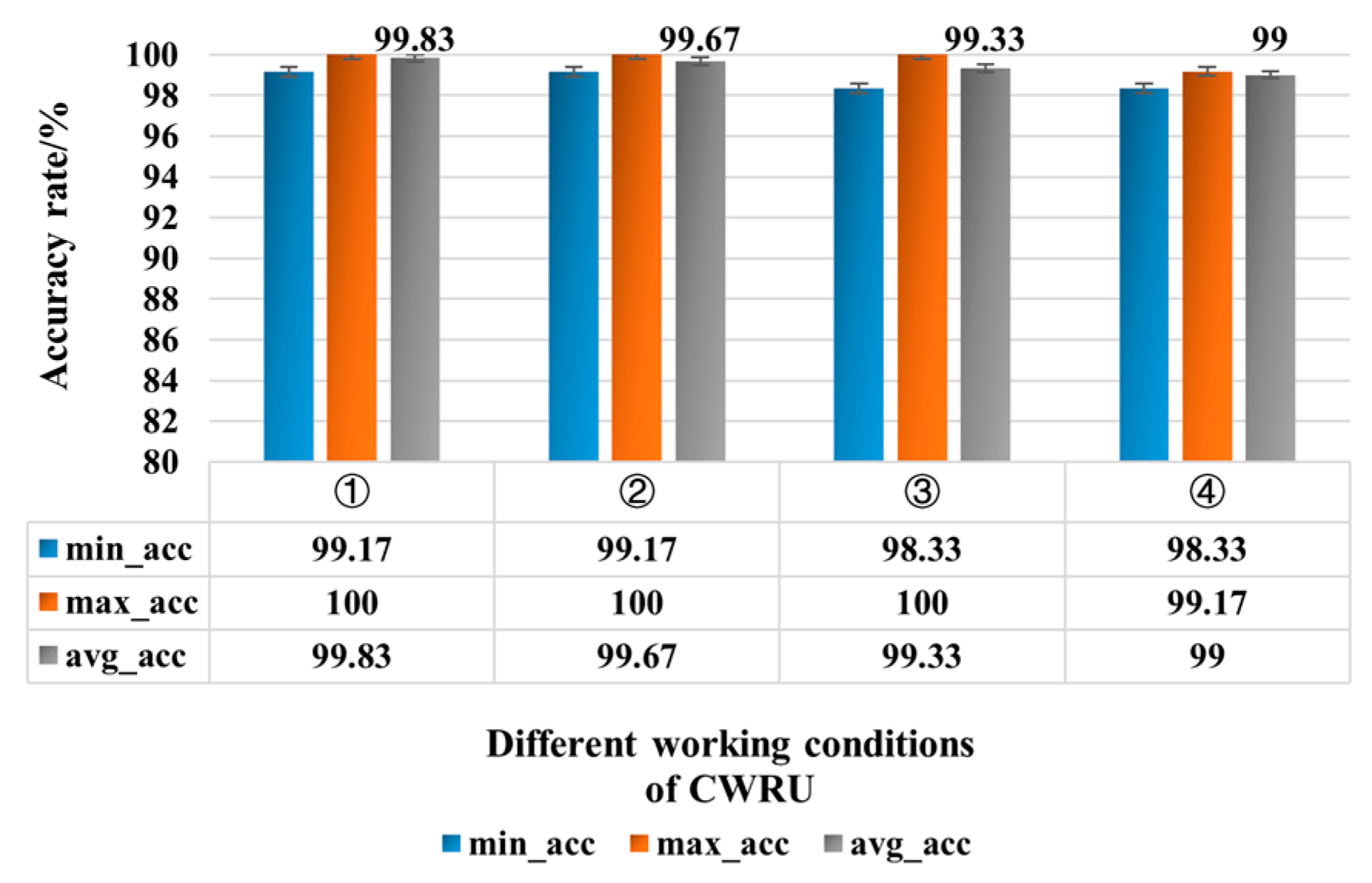
The proposed model generalization performance is further verified using the CWRU bearing fault dataset [35]. Fault tests are conducted under four different operating conditions (① speed of 1797 r/min, load of 0 HP; ② speed of 1772 r/min, load of 1 HP; ③ speed of 1750 r/min, load of 2 HP; and ④ speed of 1730 r/min, load of 3 HP); the collected signals are from the motor drive end bearings, including a total of four health states, namely normal, inner ring fault, outer ring fault, and rolling element fault; each type of fault is a single point of fault with a diameter of 0.1778 mm; and the sampling time and sampling frequency are the same as described in this paper. The measured data are preprocessed for the different state types under the four working conditions; due to the limited length of data for each state signal, each state signal is divided into 100 samples. Five training tests are conducted, respectively, and the test results are obtained as shown in Figure 21.

Under different rotational speeds and load conditions, the proposed model shows excellent performance and verifies its generalization ability under different working conditions. Specifically, when the rotational speed is 1730 r/min, the proposed model achieves an average recognition accuracy rate of 99.00%; when the rotational speed is 1750 r/min, the average recognition accuracy rate is 99.33%; when the rotational speed is increased to 1772 r/min, the average accuracy rate is as high as 99.67%; and when the rotational speed reaches 1797 r/min, the average accuracy rate is still as high as 99.83%. These results demonstrate that the optimization capability of RSNGO is not confined to specific operating conditions; the parameters obtained through optimization enable the model to extract stable fault features from open-set test data and consistently maintain high fault recognition accuracy, fully reflecting its excellent adaptability.

5. Conclusions

To address the problem of inaccurate recognition of multi-fault features in cylindrical roller bearings, a bearing multi-fault pattern recognition model based on RSNGO-optimized VMD and CNN-BiLSTM-SAT is proposed in this paper. The effectiveness of the proposed method is validated through extensive bearing fault experiments, and the following conclusions are drawn:

(1)

Compared with the NGO, PSO, WOA, and DBO algorithms, the proposed RSNGO algorithm achieves a faster convergence rate and stronger global search capability. More importantly, this optimization advantage effectively translates into enhanced feature discrimination and improved diagnostic robustness. RSNGO-VMD is employed to decompose the original vibration signals and select the optimal IMF components, which effectively suppresses environmental noise interference. Furthermore, RSNGO is utilized to optimize the hyperparameters of the CNN-BiLSTM-SAT model, enabling the construction of an optimal network architecture and effectively overcoming the limitations of traditional convolutional neural networks.

(2)

Compared with other benchmark models, the proposed method achieves more than 99% in key evaluation metrics, including macro-precision, macro-recall, and macro-F1 score, and exhibits significantly higher fault recognition accuracy. In addition, compared with other optimization algorithms, the RSNGO-optimized network model demonstrates superior recognition performance. The t-SNE visualization results further reveal that different fault categories exhibit clear clustering characteristics in the feature space, confirming the effectiveness of the proposed model in multi-fault pattern recognition.

(3)

Under noisy conditions, the proposed model exhibits strong robustness. Even at an SNR of −3 dB, the average recognition accuracy remains above 95%, demonstrating excellent noise resistance. Under different self-acquired experimental conditions, the model achieves an average recognition accuracy exceeding 99%. Furthermore, on the CWRU bearing fault dataset, the proposed model maintains high identification accuracy under all four rotational speeds, further verifying its strong adaptability to different operating conditions.

Overall, the proposed model can effectively identify multiple fault patterns of cylindrical roller bearings under different operating conditions, providing reliable technical support for bearing fault diagnosis. Future research will focus on the fusion of multi-source feature information and further investigate fault state assessment methods for cylindrical roller bearings.

References

1. Chen, X.; Yang, R.; Xue, Y.; Huang, M.; Ferrero, R.; Wang, Z. Deep transfer learning for bearing fault diagnosis: A systematic review since 2016. IEEE Trans. Instrum. Meas. 2023, 72, 1–21. [Google Scholar]
2. Barai, V.; Ramteke, S.M.; Dhanalkotwar, V.; Nagmote, Y.; Shende, S.; Deshmukh, D.S. Bearing Fault Diagnosis Using Signal Processing and Machine Learning Techniques: A Review. In IOP Conference Series: Materials Science and Engineering; IOP Publishing: Bristol, UK, 2022; Volume 1259, p. 012034. [Google Scholar]
3. Dragomiretskiy, K.; Zosso, D. Variational mode decomposition. IEEE Trans. Signal Process. 2013, 62, 531–544. [Google Scholar]
4. Zhou, Z.; Chen, W.; Yang, C. Adaptive range selection for parameter optimization of VMD algorithm in rolling bearing fault diagnosis under strong background noise. J. Mech. Sci. Technol. 2023, 37, 5759–5773. [Google Scholar] [CrossRef]
5. Li, M.; Yan, C.; Liu, W.; Liu, X.; Zhang, M.; Xue, J. Fault diagnosis model of rolling bearing based on parameter adaptive AVMD algorithm. Appl. Intell. 2022, 53, 3150–3165. [Google Scholar] [CrossRef]
6. Zhou, J.B.; Xiao, M.H.; Niu, Y.; Ji, G.J. Rolling Bearing Fault Diagnosis Based on WGWOA-VMD-SVM. Sensors 2022, 22, 6281. [Google Scholar] [CrossRef] [PubMed]
7. Dehghani, M.; Hubálovský, Š.; Trojovský, P. Northern goshawk optimization: A new swarm-based algorithm for solving optimization problems. IEEE Access 2021, 9, 162059–162080. [Google Scholar] [CrossRef]
8. Liang, Y.; Hu, X.; Hu, G.; Dou, W. An enhanced northern goshawk optimization algorithm and its application in practical optimization problems. Mathematics 2022, 10, 4383. [Google Scholar] [CrossRef]
9. Huang, Y.J.; Liao, A.H.; Hu, D.Y.; Shi, W.; Zheng, S.B. Multi-scale convolutional network with channel attention mechanism for rolling bearing fault diagnosis. Measurement 2022, 203, 111935. [Google Scholar] [CrossRef]
10. Song, B.; Liu, Y.; Fang, J.; Liu, W.; Zhong, M.; Liu, X. An optimized CNN-BiLSTM network for bearing fault diagnosis under multiple working conditions with limited training samples. Neurocomputing 2024, 574, 127284. [Google Scholar] [CrossRef]
11. Huang, D.; Su, X.; Yang, J.; Du, S.; Wang, D.; Ran, Q. An improved dual-channel CNN-BILSTM fusion attention model for fault diagnosis of aero-engine bearings. Measurement 2025, 253, 117761. [Google Scholar] [CrossRef]
12. Siddique, M.F.; Saleem, F.; Umar, M.; Kim, C.H.; Kim, J.-M. A hybrid deep learning approach for bearing fault diagnosis using continuous wavelet transform and attention-enhanced spatiotemporal feature extraction. Sensors 2025, 25, 2712. [Google Scholar] [CrossRef] [PubMed]
13. Fu, G.; Wei, Q.; Yang, Y. Bearing fault diagnosis with parallel CNN and LSTM. Math. Biosci. Eng. 2024, 21, 2385. [Google Scholar] [CrossRef] [PubMed]
14. Han, K.; Wang, W.; Guo, J. Research on a bearing fault diagnosis method based on a CNN-LSTM-GRU model. Machines 2024, 12, 927. [Google Scholar] [CrossRef]
15. Deng, X.; Wang, Y.; Meng, Q. A CNN-BiLSTM Bearing Fault Diagnosis Model Based on an Improved Grey Wolf Optimization Algorithm. Eng. Lett. 2026, 34, 1874. [Google Scholar]
16. Dong, Z.; Zhao, D.; Cui, L. An intelligent bearing fault diagnosis framework: One-dimensional improved self-attention-enhanced CNN and empirical wavelet transform. Nonlinear Dyn. 2024, 112, 6439–6459. [Google Scholar] [CrossRef]
17. Zhao, D.; Tian, C.; Fu, Z.; Zhong, Y.; Hou, J.; He, W. Multi scale convolutional neural network combining BiLSTM and attention mechanism for bearing fault diagnosis under multiple working conditions. Sci. Rep. 2025, 15, 13035. [Google Scholar] [CrossRef] [PubMed]
18. Zhang, Y.; Lin, L.; Wang, J.; Zhang, W.; Gao, S.; Zhang, Z. Attention activation network for bearing fault diagnosis under various noise environments. Sci. Rep. 2025, 15, 977. [Google Scholar] [CrossRef] [PubMed]
19. Wang, Y.; Li, D.; Li, L.; Sun, R.; Wang, S. A novel deep learning framework for rolling bearing fault diagnosis enhancement using VAE-augmented CNN model. Heliyon 2024, 10, e35407. [Google Scholar] [CrossRef] [PubMed]
20. Zhang, Y.; Li, S.; Zhang, A.; Li, C.; Qiu, L. A novel bearing fault diagnosis method based on few-shot transfer learning across different datasets. Entropy 2022, 24, 1295. [Google Scholar] [CrossRef] [PubMed]
21. Wang, H.; Wu, Z.; Rahnamayan, S.; Liu, Y.; Ventresca, M. Enhancing particle swarm optimization using generalized opposition-based learning. Inf. Sci. 2011, 181, 4699–4714. [Google Scholar] [CrossRef]
22. Mirjalili, S. SCA: A sine cosine algorithm for solving optimization problems. Knowl.-Based Syst. 2016, 96, 120–133. [Google Scholar] [CrossRef]
23. Jiang, K.; Yang, Z.; Jin, T.; Chen, C.; Liu, Z.; Zhang, B. CNN-based rolling bearing fault diagnosis method with quantifiable interpretability. IEEE Trans. Instrum. Meas. 2025, 74, 1–12. [Google Scholar] [CrossRef]
24. Shao, L.; Zhao, B.; Kang, X. Rolling Bearing Fault Diagnosis Based on VMD-DWT and HADS-CNN-BiLSTM Hybrid Model. Machines 2025, 13, 423. [Google Scholar] [CrossRef]
25. Shen, J.; Zhou, H.; Jin, M.; Jin, Z.; Wang, Q.; Mu, Y.; Hong, Z. Rul prediction of rolling bearings based on fruit fly optimization algorithm optimized CNN-LSTM neural network. Lubricants 2025, 13, 81. [Google Scholar] [CrossRef]
26. Vaswani, A.; Shazeer, N.; Parmar, N.; Uszkoreit, J.; Jones, L.; Gomez, A.N.; Kaiser, L.; Polosukhin, I. Attention is all you need. Adv. Neural Inf. Process. Syst. 2017, 30. [Google Scholar]
27. Wang, Z.; Peng, Q.; Rao, W.; Li, D. An improved sparrow search algorithm with multi-strategy integration. Sci. Rep. 2025, 15, 3314. [Google Scholar] [CrossRef] [PubMed]
28. Shen, J.; Wang, Z.; Wang, Y.; Zhu, H.; Zhang, L.; Tang, Y. AGWO-PSO-VMD-TEFCG-AlexNet bearing fault diagnosis method under strong noise. Measurement 2025, 242, 116259. [Google Scholar] [CrossRef]
29. Wang, S.; Wang, C.; Lian, Y.; Luo, B. Research on Bearing Fault Diagnosis Based on VMD-RCMWPE Feature Extraction and WOA-SVM-Optimized Multidataset Fusion. Sensors 2025, 25, 5139. [Google Scholar] [CrossRef] [PubMed]
30. Yuan, Y.; Wei, W. Fault diagnosis of wind turbine bearings based on improved dung beetle optimizer optimized LSTM. Eng. Res. Express 2025, 7, 035221. [Google Scholar] [CrossRef]
31. Wang, J.; Yuan, Y.; Zheng, W.; Wan, X.; Zhang, J. Intelligent Diagnosis of Rolling Bearings Based on Parameter-Optimized Variational Mode Decomposition and BiLSTM. In 2025 International Conference on Advanced Machine Learning and Data Science (AMLDS); IEEE: New York, NY, USA, 2025; pp. 111–116. [Google Scholar]
32. Ma, J.; Yu, S.; Cheng, W. Composite fault diagnosis of rolling bearing based on chaotic honey badger algorithm optimizing VMD and ELM. Machines 2022, 10, 469. [Google Scholar] [CrossRef]
33. Bhende, A.R. A robust XGBoost approach for bearing fault prediction from vibration signals: Feature analysis and model evaluation. Noise Vib. Worldw. 2026, 57, 120–129. [Google Scholar] [CrossRef]
34. Xiao, Z.; Cao, X.; Hao, H.; Liang, S.; Liu, J.; Li, D. A Spatio-Temporal Joint Diagnosis Framework for Bearing Faults via Graph Convolution and Attention-Enhanced Bidirectional Gated Networks. Sensors 2025, 25, 3908. [Google Scholar] [CrossRef] [PubMed]
35. Bensaoucha, S.; Gharib, G.M.; Al Soudi, M.; Teta, A.; Benzita, S.; Bertal, A.S.; Guiatni, A.; Rabehi, A.; Benghanem, M. Robust Bearing Fault Detection and Classification Using Deep Neural Networks: A Comprehensive Study on the CWRU Dataset. J. Eur. Syst. Autom. 2025, 58, 2435–2443. [Google Scholar] [CrossRef]
Figure 1. Convolutional neural network model.
Machines 14 00901 g001
Figure 2. Bidirectional long short-term memory.
Machines 14 00901 g002
Figure 3. Structure of self-attention mechanism.
Machines 14 00901 g003
Figure 4. Convergence curves of different optimization algorithms on benchmark functions.
Machines 14 00901 g004
Figure 5. Basic structure of the network model.
Machines 14 00901 g005
Figure 6. Model diagnosis flowchart.
Machines 14 00901 g006
Figure 7. Gear box bearing fault simulation test bench.
Machines 14 00901 g007
Figure 8. Actual bearings and time-domain waveforms under different conditions.
Machines 14 00901 g008
Figure 9. Slice preprocessing of signal.
Machines 14 00901 g009
Figure 10. Time-domain waveforms of the optimal IMF components for bearing data under different conditions.
Machines 14 00901 g010
Figure 11. Iteration curves of accuracy rate and loss error.
Machines 14 00901 g011
Figure 12. Impact of batch size on accuracy and running time.
Machines 14 00901 g012
Figure 13. Model diagnosis results.
Machines 14 00901 g013
Figure 14. Performance comparison of different models.
Machines 14 00901 g014
Figure 15. Comparison of confusion matrices of the compared models.
Machines 14 00901 g015
Figure 16. Comparison of different intelligent algorithms.
Machines 14 00901 g016
Figure 17. Ablation test results.
Machines 14 00901 g017
Figure 18. Model accuracy after adding noise with different signal-to-noise ratios.
Machines 14 00901 g018
Figure 19. t-SNE visualizations at various SNRs.
Machines 14 00901 g019
Figure 20. Model accuracy on self-collected data.
Machines 14 00901 g020
Figure 21. Model accuracy on the CWRU dataset.
Machines 14 00901 g021