Article

Remaining Useful Life Prediction for Rolling Bearings by Integrating Degradation Assessment with DK-Mamba


by
Yusheng Zhang
and
Zhibin Chen
*
School of Electronics and Information Engineering, University of Science and Technology Liaoning, Anshan 114051, China
*
Author to whom correspondence should be addressed.
Machines 2026, 14(8), 836; https://doi.org/10.3390/machines14080836
Submission received: 29 June 2026 / Revised: 17 July 2026 / Accepted: 21 July 2026 / Published: 23 July 2026
(This article belongs to the Section Machines Testing and Maintenance)

Abstract

Remaining useful life (RUL) prediction of rolling bearings is essential for ensuring the safe operation and condition-based maintenance of rotating machinery. To address unreliable degradation-onset identification and insufficient joint modeling of trend and detail components in non-stationary degradation signals, this paper proposes a two-stage framework that integrates degradation assessment with the DK-Mamba network. First, a multi-feature health indicator is constructed, and a dual-branch persistent validation strategy (DPV-FPT) is developed to robustly identify the first prediction time (FPT). Second, a multi-scale dynamic decomposition module is employed to adaptively separate the degradation sequence into trend and detail components. The Mamba architecture is then used to capture long-range temporal dependencies in the trend branch, while wavelet-based soft-threshold shrinkage is introduced to suppress noise-like high-frequency disturbances and JacobiKAN is employed to enhance the nonlinear representation of localized impulsive degradation features in the detail branch. Finally, a cross-attention mechanism is employed to adaptively fuse the trend and detail representations for RUL prediction. Experiments on the PHM2012 and IMS datasets demonstrate that the proposed method improves FPT identification reliability and achieves accurate and robust RUL prediction under complex degradation patterns and varying operating conditions.

1. Introduction

In modern industrial systems, rolling bearings are critical components of rotating machinery, including machine tool spindles, wind turbines, and aero-engines, and their health condition directly affects equipment reliability and operational safety. To improve maintenance efficiency and economic performance while reducing operational risks, prognostics and health management (PHM) has attracted increasing attention, with remaining useful life (RUL) prediction regarded as one of its fundamental tasks. RUL prediction aims to estimate the residual service life of equipment from historical condition-monitoring data, thereby supporting condition-based maintenance decisions, reducing unexpected downtime, and lowering maintenance costs. With advances in sensing and data acquisition technologies, data-driven methods have become an important direction for bearing RUL prediction and have demonstrated promising applicability under complex operating conditions [1]. Deep learning has further advanced this field by enabling models to automatically learn degradation-related representations with less reliance on handcrafted features and predefined rules. Nevertheless, owing to the non-stationary nature of bearing degradation signals, accurately identifying the onset of sustained degradation and effectively modeling both long-term degradation evolution and localized impulsive characteristics remain challenging for bearing RUL prediction. The degradation process of rolling bearings generally progresses from stable operation through sustained degradation to eventual failure [2]. Accordingly, bearing prognostics typically involve two closely related tasks: identifying the onset of degradation and subsequently estimating the RUL. Because signal characteristics and degradation dynamics vary across different life stages, conventional single-stage models may have difficulty simultaneously representing normal operating fluctuations and subsequent degradation evolution over the full life cycle. Two-stage prognostic frameworks address this issue by first identifying the degradation onset and then modeling the degradation stage separately [3]. Within such frameworks, the first prediction time (FPT) denotes the transition from normal operating fluctuations to sustained degradation. Its determination directly affects degradation-stage sample selection and RUL-label construction and therefore plays an important role in the overall prediction process.
Existing studies on degradation-onset identification have primarily focused on health-indicator construction, threshold design, statistical change detection, and anomaly detection. Zhao et al. [4] proposed a health-indicator-based method that jointly considers monotonicity and detectability to support both FPT identification and RUL prediction. Mi et al. [5] combined an extended isolation forest with nonparametric cumulative-sum statistics to improve early fault detection under noisy conditions while reducing false alarms. Zhang et al. [6] integrated unsupervised anomaly detection with an adaptive thresholding mechanism to achieve adaptive localization of the degradation onset and enhance sensitivity to incipient degradation characteristics. Although these studies have advanced degradation-onset identification, reliable FPT localization remains challenging for complex and non-stationary full-life vibration sequences. A transient impulse may produce an isolated threshold crossing without indicating sustained degradation, while a criterion based primarily on amplitude may not adequately characterize the local growth tendency of the degradation indicator. Moreover, insufficient persistence validation after a candidate onset has been detected may result in premature FPT localization. These limitations highlight the need for an identification strategy that jointly considers complementary degradation cues and verifies the persistence of candidate onset points.
At the RUL prediction stage, deep learning methods have been widely adopted because of their ability to automatically extract degradation-related representations from time-series data [7,8,9]. Recurrent neural networks (RNNs) and their representative variants, including gated recurrent units (GRUs) and long short-term memory (LSTM) networks, have become important baseline models for temporal degradation modeling. For example, Wang et al. [10] integrated a deep convolutional autoencoder, a multilayer bidirectional LSTM, and a temporal-pattern attention mechanism to construct degradation-related representations for bearing RUL prediction. However, when applied to non-stationary full-life degradation sequences, recurrent models may still have difficulty preserving long-range temporal dependencies and characterizing feature evolution under complex degradation patterns.
To strengthen global temporal modeling, attention-based and Transformer-based architectures have increasingly been introduced into bearing RUL prediction. Existing studies have combined temporal convolutional networks or recurrent structures with Transformer modules to capture local degradation patterns and long-range temporal dependencies simultaneously [11,12]. These methods improve the joint representation of local and global temporal information. However, they generally process the degradation sequence as an integrated representation, and the explicit separation of slowly varying degradation trends, localized impulsive variations, and stochastic high-frequency fluctuations is not their principal modeling objective.
In recent years, Mamba, an architecture based on state-space models, has provided a new perspective for efficient long-sequence modeling [13]. By introducing input-dependent selective state transitions, Mamba can represent long-range temporal dependencies with favorable computational efficiency and has therefore attracted increasing attention in prognostic applications. Yue et al. [14] combined the Mamba state-space framework with segmented physical degradation modeling and particle filtering for cutting-tool RUL prediction. Li et al. [15] integrated bidirectional Mamba with causal discovery, attention mechanisms, and LSTM for aero-engine RUL prediction. More recent studies have incorporated multi-head attention and learnable scaling parameters into Mamba-based RUL models [16] and developed the Mamba-SDP framework for multisensor rolling-bearing RUL prediction [17]. These studies indicate the potential of state-space models for long-range degradation modeling, attention enhancement, and multisensor information interaction. Nevertheless, most existing methods process degradation sequences as integrated representations, whereas the explicit decomposition and dedicated modeling of cumulative degradation trends and localized detail variations before state-space encoding remain comparatively underexplored.
In addition to long-range temporal modeling, the nonlinear representation of localized degradation details requires specific consideration. High-frequency detail components may contain both degradation-related impulses and stochastic fluctuations, and direct nonlinear encoding may cause noise-like variations to be modeled together with informative localized patterns. To mitigate this issue, wavelet soft-threshold shrinkage is first applied to attenuate noise-like high-frequency disturbances before nonlinear feature extraction. Kolmogorov–Arnold networks construct learnable nonlinear mappings through trainable univariate functions [18], while Jacobi-function-based variants provide flexible basis expansions for approximating complex nonlinear relationships [19]. However, the suitability of different nonlinear mapping modules for representing wavelet-processed degradation details remains insufficiently examined in bearing RUL prediction.
To address the above limitations, this study proposes a two-stage RUL prediction framework that integrates degradation assessment with DK-Mamba-based RUL prediction. First, a multi-feature health indicator and a dual-branch persistent validation strategy, termed DPV-FPT, are constructed to reduce false alarms caused by short-term fluctuations and transient spike-like disturbances. At the RUL prediction stage, the degradation sequence is adaptively decomposed into trend and detail components. Mamba is employed to model long-range temporal dependencies in the trend component, while wavelet soft-threshold shrinkage and JacobiKAN are used to suppress noise-like fluctuations and represent nonlinear localized degradation patterns in the detail component. A cross-attention mechanism is subsequently introduced to integrate the complementary trend and detail representations. Comparative, ablation, and nonlinear-module replacement experiments are conducted on the PHM2012 and IMS datasets to evaluate the proposed framework and examine the suitability of JacobiKAN for the high-frequency detail branch. The main contributions of this study are summarized as follows:
(1)
A degradation-onset localization strategy based on dual-branch persistent validation is proposed. By jointly considering amplitude variation, local growth tendency, short- and long-window persistence, and future-window confirmation, the proposed DPV-FPT strategy distinguishes sustained degradation from transient threshold crossings.
(2)
An adaptive trend–detail RUL modeling framework is constructed for heterogeneous bearing degradation sequences. The proposed multi-scale dynamic decomposition module separates cumulative degradation trends from localized detail variations, while a Mamba-based trend encoder captures long-range temporal dependencies in the cumulative degradation trajectory.
(3)
A detail encoder combining wavelet soft-threshold shrinkage and JacobiKAN is introduced to suppress noise-like high-frequency disturbances and represent nonlinear localized degradation patterns. The suitability of JacobiKAN for the wavelet-processed detail branch is further examined through controlled replacement experiments with a standard KAN, ChebyshevKAN, and an MLP. Cross-attention is subsequently employed to integrate complementary trend and detail information for RUL prediction.

2. Degradation Assessment and FPT Identification

2.1. Problem Definition

The full-life vibration signals collected from rolling bearings are considered in this study. Let x t ( n ) denote the vibration signal corresponding to the t t h sampling file, where t = 1 , 2 , , T denotes the time index and n = 1 , 2 , , N denotes the sampling-point index within a single file.
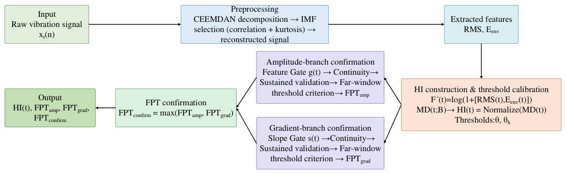
During the full-life degradation process, FPT is defined as the earliest time at which the bearing transitions from normal operating fluctuations to sustained degradation. However, owing to variations in operating conditions and short-term fluctuations in vibration signals, FPT is prone to misidentification. To address this issue, a health baseline segment is introduced to establish the baseline reference range for degradation features and the health indicator, and a dual-branch persistent validation mechanism, termed DPV-FPT, is developed to improve the reliability of degradation-onset identification. The overall procedure of degradation assessment and FPT identification is illustrated in Figure 1. First, the vibration signal is decomposed by complete ensemble empirical mode decomposition with adaptive noise (CEEMDAN), and the intrinsic mode function (IMF) components are selected according to adaptive criteria to reconstruct an enhanced signal. Then, the root mean square (RMS) and envelope energy ( E env ) are extracted from the reconstructed signal and subjected to logarithmic compression. Combined with the health baseline segment, the Mahalanobis distance MD ( t ) is constructed, from which the normalized health indicator HI ( t ) ( 0 , 1 ) is obtained. Finally, persistent validation is performed in both the amplitude branch and the gradient branch, and the confirmed degradation onset is denoted as FPT confirm .

2.2. CEEMDAN-Based Signal Enhancement

CEEMDAN was proposed by Torres et al. [20]. By progressively introducing adaptive noise at each decomposition stage, it can effectively alleviate mode mixing and reduce reconstruction error. Its main procedure is summarized as follows.
(1)
Construct the noise-assisted signal:
x t ( i ) ( n ) = x t ( n ) + ε 0 δ i ( n )
where ε 0 denotes the noise amplitude coefficient, and δ i ( n ) denotes the i-th added white-noise sequence.
(2)
Perform empirical mode decomposition (EMD) on each noise-assisted signal x t ( i ) ( n ) , and obtain the first intrinsic mode function (IMF) by averaging the first-mode components obtained from all decompositions, denoted as IMF t , 1 ( n ) = 1 I i = 1 I IMF t , 1 ( i ) ( n ) . The corresponding residual is then given by r t , 1 ( n ) = x t ( n ) IMF t , 1 ( n ) .
(3)
For higher-order components j 2 , adaptive noise is added to r t , j 1 ( n ) , after which decomposition is performed again. The averaged result yields IMF t , j ( n ) , and the residual is updated as
r t , j ( n ) = r t , j 1 ( n ) IMF t , j ( n )
(4)
The decomposition terminates when the residual exhibits a monotonic trend and can no longer be further decomposed. The original signal can then be expressed as
x t ( n ) = j = 1 J IMF t , j ( n ) + R t ( n )
where j denotes the index of IMF components, J denotes the total number of IMF components, and R t ( n ) denotes the final residual component of the t-th sampling file obtained after CEEMDAN decomposition, which mainly represents the low-frequency trend that cannot be further decomposed.
After CEEMDAN decomposition, the original signal is represented as a series of IMF components arranged from high frequency to low frequency. Among them, the high-frequency components mainly reflect localized transient oscillations and fine-scale variations, whereas the low-frequency components characterize the overall degradation trend of the signal.
To extract the effective components associated with degradation, an adaptive screening criterion jointly considering correlation and kurtosis is adopted. For the j-th IMF of the t-th sampling file, the absolute correlation coefficient between the IMF and the original signal is denoted as
c t , j = corr IMF t , j , x t ,
and the corresponding kurtosis is denoted as κ t , j . The correlation coefficients are arranged in descending order as c t , ( 1 ) c t , ( 2 ) c t , ( J ) , where J denotes the total number of IMF components.
Given the correlation-ranking ratio ρ c , the ranking position is defined as
r = max 1 , round ( ρ c J ) .
The adaptive correlation threshold is then determined as
c th , t = min max c t , ( r ) , c min , c max ,
where c min and c max denote the lower and upper bounds of the adaptive correlation threshold, respectively. The retained IMF index set is defined as
Ω t = j c t , j c th , t or κ t , j κ th ,
where κ th denotes the kurtosis threshold. Finally, the retained IMF components are superimposed to reconstruct the enhanced signal for subsequent feature extraction:
x ˜ t ( n ) = j Ω t IMF t , j ( n ) .

2.3. Feature Extraction and Preprocessing

For the reconstructed signal x ˜ t ( n ) of the t-th sampling file, a two-dimensional degradation feature vector is extracted as f ( t ) = [ RMS ( t ) , E env ( t ) ] T . Among these features, RMS is used to characterize the signal energy level and is defined as:
RMS ( t ) = 1 N n = 1 N x ˜ t 2 ( n )
The envelope energy E env ( t ) is used to characterize the intensity of impulsive envelopes. Let e t ( n ) = x ˜ t ( n ) + i H x ˜ t ( n ) denote the envelope obtained from the analytic signal, where H { · } denotes the Hilbert transform. Then, the envelope energy is defined as
E env ( t ) = 1 N n = 1 N e t 2 ( n )
Considering that extreme peaks may appear in the later stage of bearing degradation and may adversely affect threshold setting and scale normalization, the two-dimensional features are compressed using the log1p transformation:
RMS ( t ) = log 1 + max RMS ( t ) , 0
E env ( t ) = log 1 + max E env ( t ) , 0
Then, the transformed feature vector f ( t ) = RMS ( t ) , E env ( t ) T is taken as the input for subsequent health indicator construction.

2.4. Health Indicator Construction via MD

To eliminate dimensional inconsistency and fuse the RMS and E env components in the feature vector f ( t ) , the Mahalanobis distance (MD) [21] is employed to construct the health indicator. By exploiting the covariance structure of the feature space, the Mahalanobis distance can jointly account for both scale differences and inter-feature correlations, thereby yielding a unified and robust degradation indicator.
Considering that vibration fluctuations are relatively large during equipment start-up and the running-in stage, the initial ρ skip proportion of samples is first excluded to avoid interference with health baseline determination. Thereafter, a healthy segment with length ratio ρ b is selected as the baseline:
t 0 = ρ skip T + 1
T b = ρ b T
where T denotes the number of sampling files in the full-life-cycle sequence, ρ skip denotes the proportion of samples excluded to avoid the start-up and running-in stage, and ρ b ( 0 , 1 ) denotes the length ratio of the health baseline segment. Here, t 0 represents the starting point of the baseline segment, and B denotes the time-index set of the health baseline segment, i.e., B = { t 0 , t 0 + 1 , , t 0 + T b 1 } .
Let the baseline feature sample set be denoted as f ( t ) t B , whose mean vector and covariance matrix are μ B and Σ B , respectively. For an arbitrary time step t, the Mahalanobis distance is defined as
D 2 ( t ) = f ( t ) μ B T Σ B 1 f ( t ) μ B
MD ( t ) = D 2 ( t )
Let the Mahalanobis distance sequence on the baseline segment be denoted as MD ( t ) t B . To construct a stable normalization scale, define
m d base = median MD ( t ) t B
m d max = Q q MD ( t ) t = 1 T
where Q q ( · ) denotes the quantile operator, and q ( 0 , 1 ) is used to determine the upper bound for normalization. To mitigate the influence of extreme peaks in the late degradation stage on the overall normalization range, MD ( t ) is upper-bounded as:
MD clip ( t ) = min MD ( t ) , m d max
Based on this, the normalized health indicator (HI) is constructed as:
H I ( t ) = min 1 , max 0 , M D clip ( t ) m d base m d max m d base + ε
where ε is a small positive constant used to avoid division by zero.
In this way, the two-dimensional degradation features are transformed into a scalar health indicator with improved robustness and comparability, which provides the basis for the subsequent DPV-FPT-based degradation-onset identification.

2.5. DPV-FPT Criterion

As illustrated in Figure 1, a dual-branch confirmation strategy combining an amplitude branch and a gradient branch is adopted to identify the degradation onset. In both branches, persistence constraints, persistent validation constraints, and future-window exceedance constraints are jointly introduced to reduce false alarms caused by short-term fluctuations and transient spike-like disturbances. The final output is the confirmed FPT, denoted as F P T confirm .
On the baseline segment B, let H I B = H I ( t ) t B . The baseline median and median absolute deviation are defined as:
m B = median H I ( t ) t B
M A D B = median H I ( t ) m B t B
where M A D B is used as a robust dispersion measure for threshold calibration. To improve the adaptivity of threshold setting, the primary threshold is computed by combining baseline statistics with a predefined upper bound θ cap :
θ ˜ = max Q 1 α H I B , m B + K f · M A D B
θ = min θ ˜ , θ cap
Furthermore, to enhance the discriminative stability of the subsequent validation stage, a margin m is introduced on the basis of the primary threshold, and the upper bound θ hcap is used for truncation to obtain the high threshold θ h :
θ h = min θ + m , θ hcap
where Q 1 α ( · ) is the ( 1 α ) -quantile of the baseline segment H I B , α controls the threshold sensitivity, K f is the MAD scaling factor, θ cap is the upper bound of the primary threshold, m is the high-threshold margin, and θ hcap is the upper bound of the high threshold.
Within the search interval T st , T ed , each candidate time t is sequentially examined. The earliest candidate time satisfying the following conditions in the amplitude branch is defined as F P T amp :
(1)
Feature gating constraint: For a candidate time t, the feature-gating window is defined as:
W g ( t ) = t , t + 1 , , min t + T g 1 , T
Within this window, the exceedance state of a single-point feature is defined as:
b i = I Z rms ( i ) > γ Z env ( i ) > γ
where I ( · ) denotes the indicator function, which equals 1 if the condition is satisfied and 0 otherwise. Then, the proportion of exceedance points within the window is required to be no smaller than the preset threshold η g :
g ( t ) = 1 W g ( t ) i W g ( t ) b i η g
(2)
Persistence constraint: The health indicator is required to continuously exceed the primary threshold over the persistence interval, i.e., H I ( i ) > θ , i t , t + 1 , , t + T c 1 ;
(3)
Persistent validation constraint: Within the short window W s ( t ) = t , , t + T s 1 , the proportion of points whose health-indicator values exceed the high threshold θ h must be no smaller than η s .
1 W s ( t ) i W s ( t ) I H I ( i ) > θ h η s
Meanwhile, within the long window W l ( t ) = t , t + 1 , , t + T l 1 , the mean value of the health indicator must exceed the high threshold θ h
1 W l ( t ) i W l ( t ) H I ( i ) > θ h
(4)
Future-window exceedance requirement: Within the future window W f ( t ) = t , t + 1 , , t + T f 1 , the proportion of points whose health-indicator values exceed the primary threshold θ must be no smaller than η f
1 W f ( t ) i W f ( t ) I H I ( i ) > θ η f
where W s ( t ) , W l ( t ) , and W f ( t ) denote the short window, long window, and future window, respectively, T s , T l , and T f are the corresponding window lengths, η s and η f are the corresponding proportion thresholds, θ is the primary threshold and θ h is the high threshold.
In the gradient branch, a slope coefficient s ( t ) is estimated by fitting a first-order linear regression model to H I ( t ) within a sliding window. This coefficient is used to characterize the local increasing trend of the health indicator, and the corresponding threshold θ g is calibrated from the baseline segment. When s ( t ) > θ g , and the persistence and validation constraints are simultaneously satisfied, the gradient-branch onset F P T grad is obtained. The final FPT is defined as:
F P T confirm = max F P T grad , F P T amp
In this study, DPV-FPT is implemented as an offline degradation-onset localization procedure for complete run-to-failure sequences. Its global hyperparameters are prespecified independently of the test-bearing RUL labels and kept fixed across all bearing sequences, whereas the bearing-specific baseline statistics and adaptive thresholds are calculated from the predefined initial healthy segment of each bearing without using RUL labels. The subsequent validation windows are used to confirm the persistence of degradation after a candidate onset.
y ( t ) = 1 , t t FPT , T t T t FPT , t FPT < t T .
Based on the two-stage degradation modeling framework, F P T confirm is taken as the starting point of the bearing degradation stage. Samples before this point are regarded as being in the healthy state, whereas samples after this point are assumed to degrade linearly until failure. Let the length of each full-life bearing sequence be T, with time index t = 1 , 2 , , T . Then, the normalized RUL label y ( t ) [ 0 , 1 ] is defined by Equation (29).

2.6. Feature Selection

In the RUL prediction stage, to characterize the amplitude variation, distributional features, complexity, and spectral-structure information during the bearing degradation process, statistical features are constructed from sliding-window segments, as listed in Table 1. A total of 15 candidate features is selected, covering indicators from the time domain, frequency, and complexity domains.
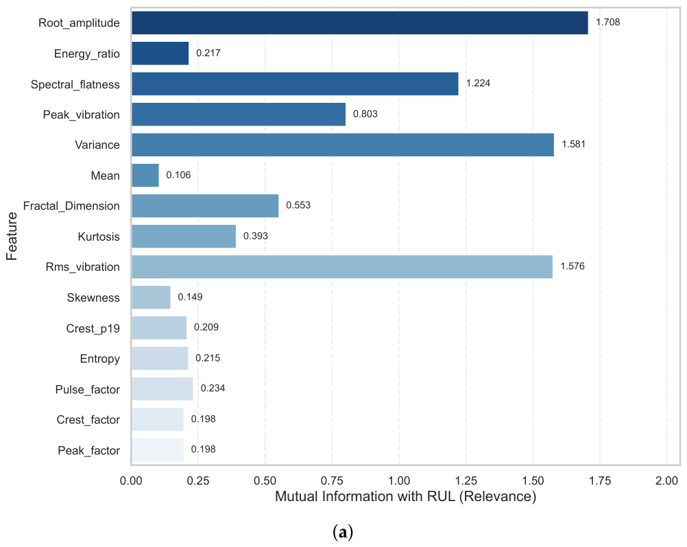
Considering both the relevance of candidate features to the RUL labels and the redundancy among features, the Minimum Redundancy Maximum Relevance (mRMR) criterion [22] based on mutual information is adopted for feature selection. Specifically, M I ( f i ; f j ) is used to measure the redundancy between features. The scoring function is defined as:
J ( f ) = MI ( f ; y ) 1 | S | s S MI sym ( f ; s )
During the search process, a Sequential Forward Selection (SFS) strategy [23] is employed to progressively incorporate features. First, the feature with the largest M I ( f ; y ) is selected. Subsequently, at each step, the next feature is determined by maximizing the scoring function, thereby yielding the feature-importance ranking. By jointly considering feature relevance and redundancy, the final input feature set is obtained.

3. Methodology

3.1. Framework Overview

Let the full-life-cycle bearing dataset be denoted as D = X ( i ) , Y ( i ) i = 1 N . In this study, a sliding-window strategy is adopted to generate training samples. At time step t, the input window is denoted as X t R L × C where L is the historical observation length and C is the feature dimension. The model learns a nonlinear mapping F Θ : R L × C R P to output the future P-step RUL prediction sequence:
Y ^ t = F Θ ( X t ) = y ^ t + 1 , , y ^ t + P
where Θ denotes the set of learnable model parameters, and P denotes the number of prediction steps. During the testing and visualization stages, the mean value of the P-step predictions is taken as the final RUL estimate for the current window, and the corresponding labels are processed in the same manner.
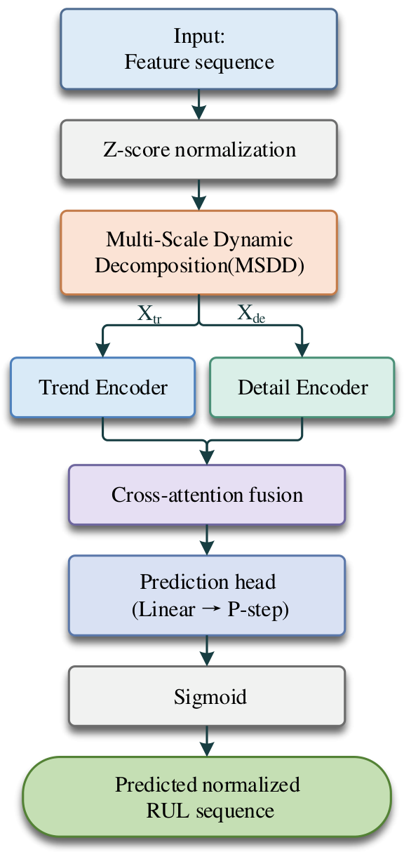
A Decomposition-KAN-Mamba prediction framework, termed DK-Mamba, is proposed in this study. As illustrated in Figure 2, the DK-Mamba framework consists of three main modules: a Multi-Scale Dynamic Decomposition (MSDD) module, a Trend–Detail Encoding module, and a Cross-Attention Fusion and Prediction module.
First, the input sequence is adaptively decomposed into a trend component X tr and a detail component X de , which represent the long-term degradation trend and the high-frequency impulsive degradation features, respectively. The trend component X tr is then fed into a Mamba-based trend encoder to capture the long-range dependencies embedded in the cumulative degradation trajectory. The resulting trend representation is denoted as H trend , i.e., H trend = Mamba X tr .
Next, the detail component X de is processed by the Detail Encoder for joint modeling in the time-domain and frequency-domain branches. Meanwhile, wavelet soft-threshold shrinkage is introduced to impose adaptive constraints on the high-frequency detail component.
Finally, a cross-attention mechanism is employed to interactively fuse the trend and detail features, and the prediction head outputs the final RUL prediction results.

3.2. Multi-Scale Dynamic Decomposition

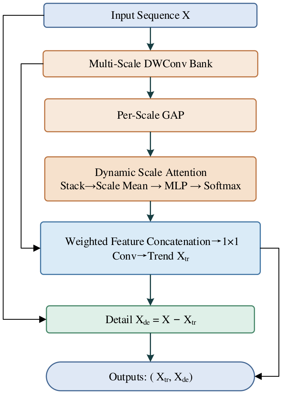
Bearing degradation signals usually contain both global degradation trends and localized impulsive degradation features. However, traditional decomposition methods based on fixed windows and fixed weights are often inadequate for capturing multi-scale temporal characteristics and may lead to information loss. To address this issue, a Multi-Scale Dynamic Decomposition module, abbreviated as MSDD, is designed, as illustrated in Figure 3.
First, the input X R B × L × C is transposed into the channel-first form required for one-dimensional convolution, yielding X c R B × C × L , where B, L, and C denote the batch size, sequence length, and feature dimension, respectively. A set of M convolution kernels with different receptive fields is predefined as K = k 1 , k 2 , , k M , together with the corresponding dilation-rate set D = d 1 , d 2 , , d M , where M denotes the number of multi-scale convolution branches. Multi-scale feature representations are then extracted through parallel depthwise dilated convolutions:
F i = DWConv k i , d i X c R B × C × L , i = 1 , 2 , , M
Next, global average pooling is applied along the temporal dimension of each scale-specific feature F i to obtain the corresponding scale descriptor p i . The scale descriptors are then stacked along the scale dimension and averaged to obtain an aggregated descriptor p ¯ . Subsequently, a lightweight multilayer perceptron is employed to generate the scale-specific scores, which are normalized by a softmax function to obtain the dynamic scale weights α = [ α 1 , α 2 , , α M ] :
p i = GAP F i R B × C ,           i = 1 , 2 , , M P = Stack i = 1 M p i R B × M × C   p ¯ = Mean scale P = 1 M i = 1 M p i R B × C   α = softmax MLP p ¯ = [ α 1 , α 2 , , α M ] R B × M  
where p i denotes the global descriptor of the ith scale, P denotes the stacked scale-descriptor tensor, and p ¯ denotes the descriptor obtained by averaging across the scale dimension. The weight α i represents the sample-dependent importance assigned to the ith scale and is broadcast along the channel and temporal dimensions when weighting F i .
i = 1 M α i = 1
Finally, each scale-specific feature F i is multiplied by its corresponding dynamic weight α i . The weighted multi-scale features are concatenated along the channel dimension and subsequently mapped through a 1 × 1 pointwise convolution to obtain the channel-first trend representation:
X tr , c = PWConv 1 × 1 Concat i = 1 M α i F i R B × C × L
The trend representation is then transposed back to the original sequence-first format:
X tr = TransposeBack X tr , c R B × L × C
The detail component is obtained as the residual between the input sequence and the extracted trend component:
X de = X X tr R B × L × C
In this way, the input sequence is adaptively decomposed into the trend component X tr and the detail component X de .

3.3. Detail Branch Encoder

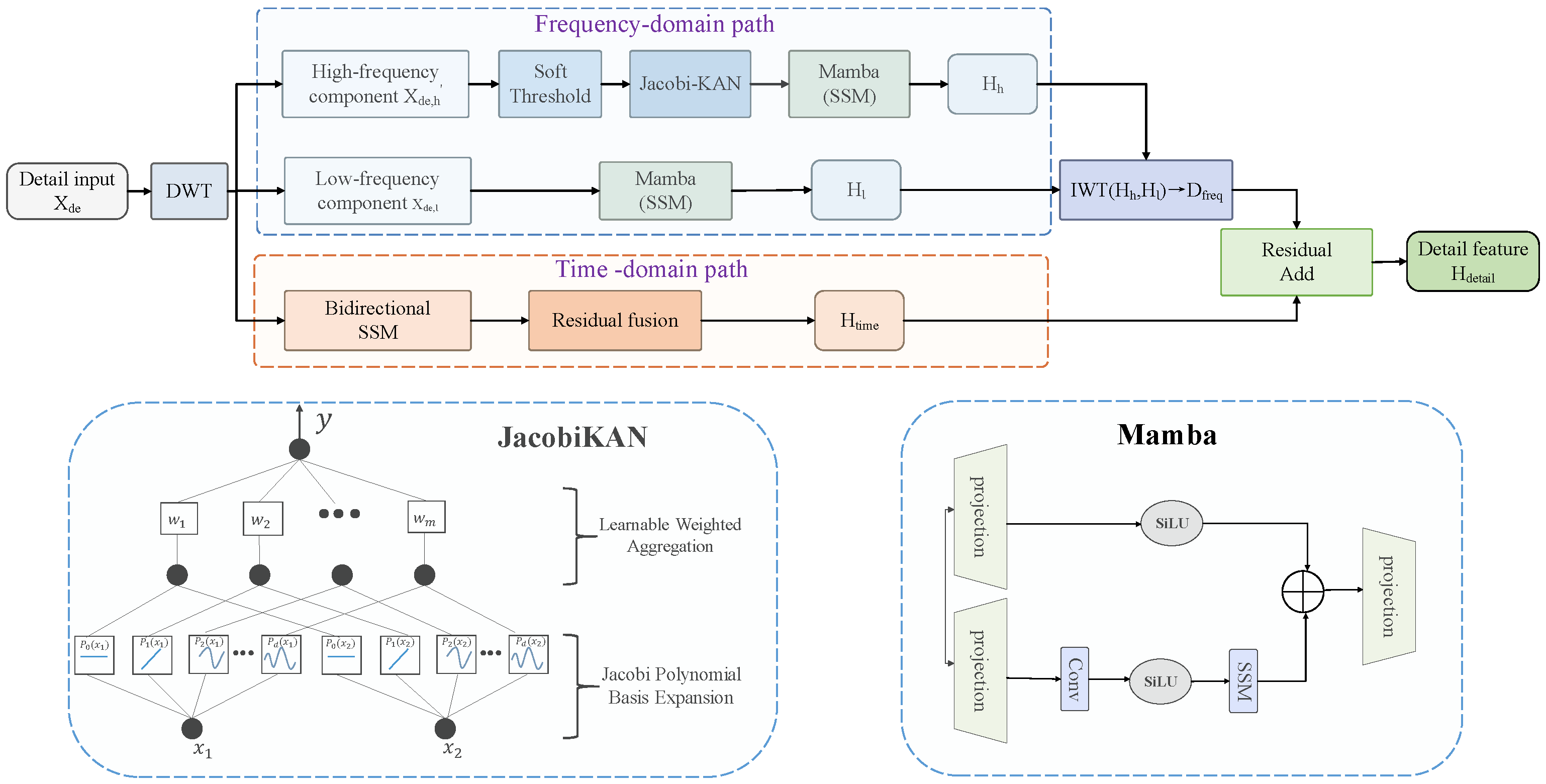
The detail component contains both early fault-induced impulses and high-frequency stochastic disturbances. If modeled directly, localized impulsive patterns are easily contaminated by short-term fluctuations. To address this issue, a Detail Encoder is designed, as illustrated in Figure 4. It consists of two parts: a frequency-domain dual-branch structure based on wavelet decomposition and a parallel time-domain contextual modeling branch built upon a Bidirectional State Space Model (Bi-SSM) [24].
First, the Discrete Wavelet Transform (DWT) is employed to decompose X de into a low-frequency component X de , l and a high-frequency component X de , h . To suppress transient spike-like disturbances and high-frequency stochastic noise in X de , h , a learnable soft-threshold shrinkage operation is introduced:
τ = σ ( θ ) · mean X de , h
X ˜ de , h = sign X de , h · max X de , h τ , 0
where θ is a learnable parameter and σ ( · ) denotes the Sigmoid function, which constrains the threshold scaling factor to the interval ( 0 , 1 ) .
To further enhance the nonlinear representation capability of the high-frequency branch, JacobiKAN [25] is introduced in the detail encoder. Compared with an MLP based on learnable affine transformations and fixed activation functions, JacobiKAN parameterizes univariate nonlinear mappings using learnable Jacobi polynomial basis expansions, thereby providing a flexible representation for complex localized impulsive degradation features.
The suitability of JacobiKAN is further evaluated through controlled replacement experiments with a standard KAN, ChebyshevKAN, and an MLP, as reported in Section 4.2.
Since the low-frequency branch mainly preserves slowly varying degradation information, it is directly fed into Mamba for sequence modeling.
By contrast, the high-frequency branch mainly contains localized impulsive degradation features and abrupt high-frequency transients. Therefore, the high-frequency branch is first enhanced by JacobiKAN to strengthen the nonlinear representation of localized impulsive degradation features, and is then fed into Mamba to capture the long-range dependencies embedded in the high-frequency detail sequence:
H l = Mamba X de , l
H h = Mamba Φ JacobiKAN X ˜ de , h
To compensate for the potential loss of temporal information caused by the frequency-domain transformation, an additional time-domain contextual modeling branch is introduced in parallel with the frequency-domain wavelet branch. In this branch, a bidirectional state space model (Bi-SSM) is employed to capture both forward and backward contextual dependencies, and the resulting features are integrated through a residual connection to obtain the time-domain representation.
H time = F X de + FlipBack F Flip X de + X de
Finally, the outputs of the low-frequency branch and high-frequency branches are reconstructed by the Inverse Wavelet Transform (IWT) and further combined with the output of the time-domain branch to obtain the final detail representation:
H detail = IWT H l , H h + H time
The overall architecture of the detail encoder, together with the JacobiKAN and Mamba modules, is illustrated in Figure 4.

3.4. Cross-Attention Fusion and RUL Prediction

Traditional dual-branch models usually fuse the trend component and the detail component through simple element-wise addition, which makes it difficult to characterize the stage-dependent evolution of localized impulsive degradation features. To address this issue, a Cross-Attention Fusion mechanism is introduced. In this module, the output of the detail encoder H detail is used as the query(Q), while the trend feature H trend serves as the key(K) and value(V), thereby enabling cross-attentive fusion between localized impulsive degradation features and the global degradation trend:
Q = H detail W Q
K = H trend W K
V = H trend W V
H att = Softmax Q K T d k V
Z = LayerNorm H detail + H att
In the prediction head, the fused feature is flattened and mapped to a P-step output. Since normalized RUL labels are adopted, a Sigmoid function is finally used to constrain the prediction results to the interval [ 0 , 1 ] :
Y ^ RUL = σ Linear Flatten Z

3.5. Evaluation Metrics

To evaluate the predictive performance of the proposed model, the Mean Absolute Error (MAE) and Root Mean Square Error (RMSE) are adopted as evaluation metrics.
Among them, MAE is used to measure the average absolute deviation between the predicted values and the ground-truth values, and is defined as
M A E = 1 n i = 1 n y i y ^ i
RMSE is used to measure the overall prediction error, and is defined as
R M S E = 1 n i = 1 n y i y ^ i 2
where y i denotes the ground-truth RUL y ^ i denotes the predicted RUL, and n denotes the number of samples. In general, smaller values of MAE and RMSE indicate better predictive performance.

4. Experimental Results

4.1. Experimental Settings on PHM2012

To verify the effectiveness of the proposed method on full-life bearing degradation sequences, experiments were conducted on the accelerated degradation dataset of rolling bearings from the IEEE PHM2012 Prognostics Challenge (PRONOSTIA platform) [26]. The platform consisted of a rotation module, a degradation loading module, and a measurement module. High-frequency accelerometers were used to collect vibration signals at a sampling frequency of 25.6 kHz, and a signal segment of length 0.1 s was acquired every 10 s. In this study, the horizontal vibration signals collected under Operating Condition 1 and Operating Condition 3 were selected and analyzed. Among them, Bearing1_3, Bearing1_5, Bearing1_6, and Bearing1_7 under Operating Condition 1, together with Bearing3_2 under Operating Condition 3, were used as the test set, while the remaining bearings were used for training.
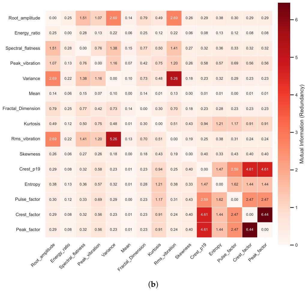
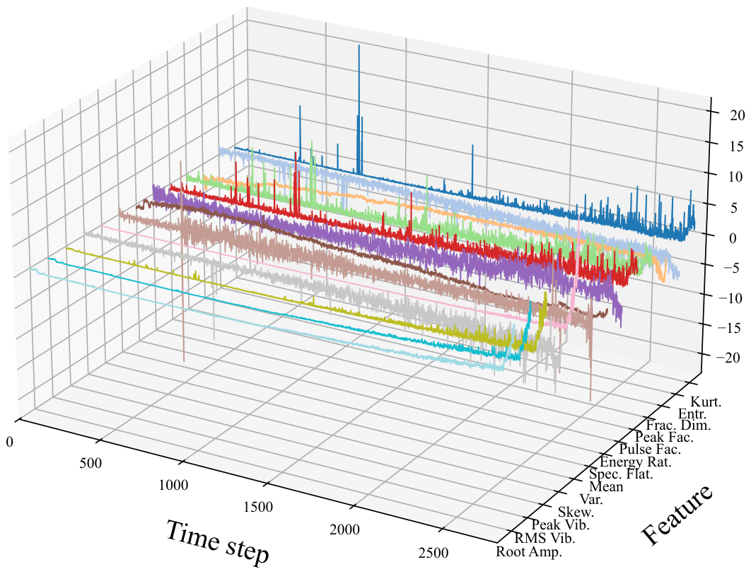
The bearing-level training–test split was completed before feature selection and normalization. The mRMR ranking was obtained using only the candidate features and RUL labels of the training bearings, and the resulting feature subset was subsequently fixed and applied unchanged to all test bearings. Based on the mRMR ranking and redundancy analysis, the p-norm Crest Factor and Margin Factor were removed, and the remaining 13 features were retained as inputs to the RUL prediction model, i.e., C = 13 . The means and standard deviations used for Z-score normalization were estimated from the concatenated feature samples of all training bearings and subsequently applied unchanged to the test bearings. The selected feature curves and the mRMR-based redundancy analysis are presented in Figure 5 and Figure 6.
A sliding-window strategy was then adopted to generate sequential samples. Specifically, a historical feature sequence of length L = 128 (with feature dimension C = 13 ) was used as the input to predict the normalized RUL at P = 4 steps ahead. To match the normalized RUL labels, a Sigmoid function was employed at the end of the prediction head to constrain the output range.
For CEEMDAN-based signal enhancement, the ensemble size, i.e., the number of noise realizations, was set to I = 50 , the relative noise amplitude was set to ε 0 = 0.2 , and the maximum number of sifting iterations was set to 100. For IMF selection, the correlation-ranking ratio was set to ρ c = 0.40 , the lower and upper bounds of the adaptive correlation threshold were set to c min = 0.15 and c max = 0.60 , respectively, and the kurtosis threshold was set to κ th = 3.0 .
In the degradation assessment and DPV-FPT decision process, the initial ρ skip = 0.05 proportion of each full-life sequence was excluded, and the baseline length ratio was set to ρ b = 0.20 . All window lengths were determined relative to the total number of sampling files T in each bearing sequence and rounded to the nearest integer. Specifically, the feature-gating, continuity, short-term validation, long-term validation, and future-validation window lengths were set to T g = 0.10 T , T c = 0.02 T , T s = 0.10 T , T l = 0.03 T , and T f = 0.20 T , respectively. The corresponding proportion thresholds were set to η g = 0.25 , η s = 0.60 , and η f = 0.75 .
The MAD scaling factor was set to K f = 0.50 . The high-threshold margin and the upper bound of the high threshold were set to m = 0.020 and θ h cap = 0.99 , respectively. The quantile parameter used to determine the upper normalization bound of the Mahalanobis distance was set to q = 0.995 , and the feature-gating threshold was set to γ = 2.5 . For primary-threshold calibration, the sensitivity parameter and the upper bound were set to α = 0.015 and θ cap = 0.95 , respectively. In the gradient branch, the slope s ( t ) was estimated using sliding-window linear regression with a window length of 0.03 T , and the gradient threshold was determined from the baseline segment according to θ g = μ g + 3 σ g .
During the training stage of the RUL prediction model, Adam was adopted as the optimizer, and the Mean Squared Error (MSE) was used as the loss function. The model was trained for 20 epochs with a batch size of 64 and an initial learning rate of 5 × 10 5 . The dropout rate was set to 0.1, the state dimension of the Mamba module was set to 32, and the convolution dimension was set to 4. Model parameters were optimized by minimizing the MSE between the predicted RUL values and the normalized ground-truth labels, while an L2 regularization term was introduced to alleviate overfitting. All models were implemented in PyTorch (version 2.10.0+cu128, CUDA 12.8) and trained on a single NVIDIA Tesla T4 GPU.

4.2. Results on the PHM2012 Dataset

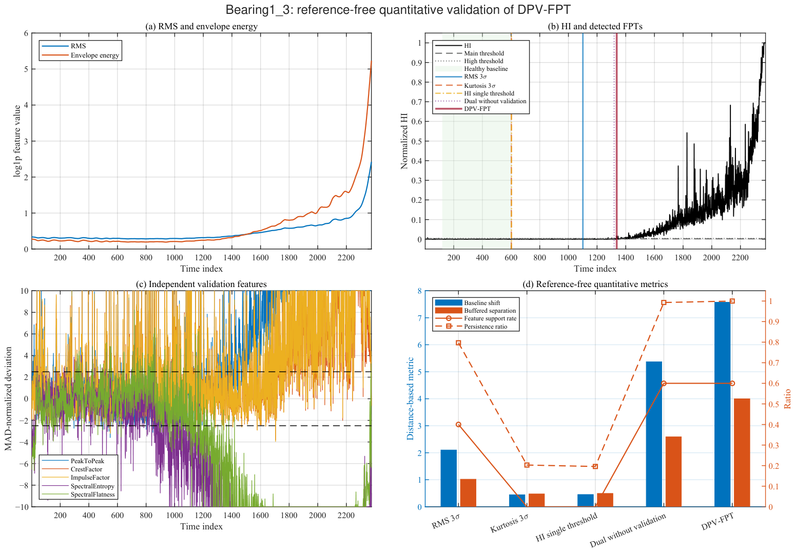
First, RMS and envelope energy E env were calculated, and the corresponding health indicator (HI) was constructed. Because the PHM2012 dataset does not provide manually annotated degradation-onset times, direct FPT localization errors cannot be calculated. Therefore, a reference-free quantitative consistency evaluation was conducted using independent features that were not involved in HI construction. The statistical consistency of the detected FPTs was evaluated in terms of state deviation, separation before and after the detected point, and degradation persistence.
The proposed DPV-FPT method was compared with the RMS-based 3 σ method, the kurtosis-based 3 σ method, the HI single-threshold method, and a dual-branch variant without persistent validation. Peak-to-peak value, crest factor, impulse factor, spectral entropy, and spectral flatness were employed as independent validation features. The detected FPTs were evaluated using the mean baseline shift, mean buffered separation, feature support rate, persistence ratio, and relapse ratio.
As shown in Figure 7 and Table 2, the kurtosis-based 3 σ method and the HI single-threshold method identified FPTs at time indices 602 and 603, respectively. However, their feature support rates were both zero, and their persistence ratios were only 0.203 and 0.196, whereas their relapse ratios reached 0.797 and 0.804, respectively. The HI also remained close to the healthy baseline level for a relatively long period after these early detections. These results indicate that the detected points were mainly associated with transient threshold crossings rather than a sustained degradation-state transition.
The RMS-based 3 σ method identified the FPT at index 1101. Although its persistence ratio increased to 0.797, its mean baseline shift, mean buffered separation, and feature support rate were only 2.104, 1.022, and 0.40, respectively. The dual-branch variant without persistent validation identified a candidate degradation point at index 1319, whereas the complete DPV-FPT method confirmed the FPT at index 1343.
The FPT identified by DPV-FPT achieved a mean baseline shift of 7.578, a mean buffered separation of 4.002, a feature support rate of 0.60, a persistence ratio of 1.000, and a relapse ratio of zero. Compared with the dual-branch variant without persistent validation, the mean baseline shift and mean buffered separation were 41.1% and 54.5% higher, respectively. These results indicate that the persistent-validation mechanism reduces premature detections caused by transient fluctuations and identifies an operational degradation boundary followed by a stronger and more persistent multi-feature state deviation. The detected point is therefore interpreted as a statistically supported operational degradation boundary rather than a uniquely defined physical degradation onset.
Table 3 further summarizes the DPV-FPT localization results for all bearing sequences in the PHM2012 dataset. The differences in the detected FPT locations indicate that the bearing sequences exhibit heterogeneous degradation durations and evolution patterns.
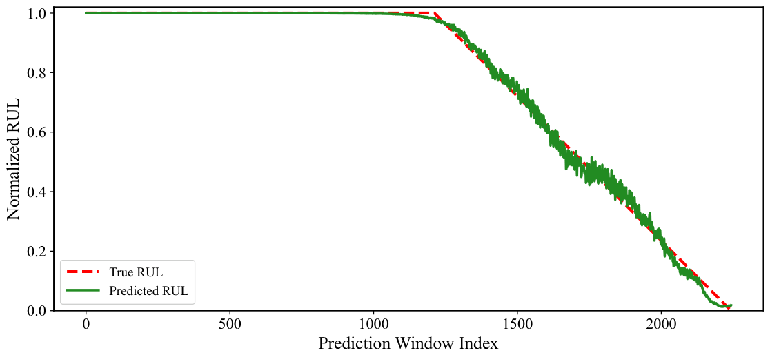
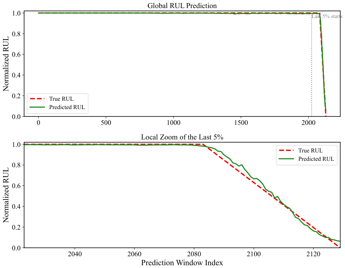
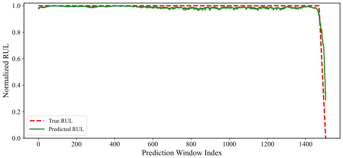
After FPT localization, RUL prediction experiments were further conducted on the test bearings in the PHM2012 dataset. Figure 8, Figure 9 and Figure 10 present the comparison curves between the predicted RUL and the true RUL for several representative bearings. Here, the horizontal axis denotes the sliding-window sample index, which reflects the degradation evolution over the bearing life. As can be seen from the figures, the proposed model generally follows the true RUL trajectories well. During the degradation stage, the predicted curves maintain a consistent downward trend with the ground-truth curves and remain relatively close to the true values before failure.
The locally enlarged view in Figure 9 further highlights that, once the bearing enters the post-FPT degradation stage, the predicted trajectory decreases consistently with the true RUL curve, indicating that the proposed model is able to effectively track the downward evolution of the degradation process. These results demonstrate that the proposed method can effectively capture the degradation evolution of rolling bearings and yield favorable RUL prediction performance for different test bearings.
Furthermore, RMSE and MAE are adopted as evaluation metrics, and Table 4 summarizes the prediction errors for all test bearings. The results indicate that the proposed model achieves low prediction errors on multiple test bearings, demonstrating favorable predictive performance on the PHM2012 dataset.
To further verify the effectiveness of the proposed method, comparisons with existing studies were conducted on the PHM2012 dataset, and the results are shown in Table 5. Here, the best results are highlighted in bold, and the second-best results are underlined. It can be seen that the proposed method is overall superior in terms of RMSE and MAE, and achieves lower prediction errors on test bearings such as Bearing1_3, Bearing1_5, and Bearing1_7, demonstrating favorable predictive performance on the RUL prediction task of the PHM2012 dataset. Compared with existing methods, the proposed method can better balance the global degradation trend and localized impulsive degradation features, thereby exhibiting better prediction performance over full-life degradation sequences.
To evaluate the contribution of each component, three ablation experiments were conducted under the same training configuration by removing MSDD, JacobiKAN, and the wavelet module, respectively. As shown in Table 6, the effects of these modules differ across evaluation metrics and test bearings. In this table, the lowest value for each evaluation metric is highlighted in bold, whereas the second-lowest value is underlined. Lower RMSE and MAE values indicate better predictive performance. The complete model achieves the lowest average RMSE of 0.0204 while maintaining a comparable average MAE of 0.0100.
Removing MSDD increases the average RMSE from 0.0204 to 0.0615 and the average MAE from 0.0100 to 0.0211. Moreover, both metrics deteriorate for all three test bearings, indicating that MSDD provides the most consistent contribution among the examined modules. This result is consistent with its intended role in separating the cumulative degradation trend from localized detail variations.
After removing the wavelet module, the average RMSE and MAE increase to 0.0266 and 0.0120, respectively, and higher RMSE values are observed for all three test bearings. Nevertheless, the MAE of Bearing1_3 decreases slightly from 0.0102 to 0.0096. These results indicate that the aggregate errors are lower when the wavelet module is included, although its effect is not uniform across every bearing and evaluation metric. This variation may reflect a trade-off between attenuating noise-like high-frequency disturbances and preserving weak degradation-related details.
Removing JacobiKAN increases the average RMSE from 0.0204 to 0.0317, with higher RMSE values observed for all three test bearings. In contrast, the average MAE changes only marginally from 0.0100 to 0.0099. Because RMSE assigns greater weight to relatively large prediction errors, this metric-dependent result suggests that the contribution of JacobiKAN is more clearly reflected in the reduction in RMSE, which may indicate improved control of relatively large prediction deviations, whereas its effect on MAE varies across individual bearing sequences. Overall, the ablation results show that MSDD provides the most consistent contribution, while the effects of the wavelet module and JacobiKAN depend on the evaluation metric and the individual bearing sequence.
To compare different nonlinear mapping modules and further examine the suitability of JacobiKAN for the high-frequency detail branch, controlled nonlinear-module replacement experiments were conducted on Bearing1_3, Bearing1_7, and Bearing3_2. In three separate experiments, JacobiKAN was replaced with a standard KAN, ChebyshevKAN, or an MLP. The replacement modules retained the same input and output dimensions, while all other model components, data partitions, preprocessing procedures, input features, and training settings were kept unchanged. The corresponding results are summarized in Table 7.
As shown in Table 7, bold values indicate the lowest value for each evaluation metric and therefore represent the best performance. Lower RMSE and MAE values indicate better predictive performance. JacobiKAN achieves the lowest average RMSE of 0.0204. Compared with KAN and ChebyKAN, it reduces the average MAE by 33.98% and 14.64%, respectively, and the average RMSE by 38.02% and 14.11%, respectively. Although the MLP obtains a slightly lower average MAE of 0.0098, its average RMSE increases to 0.0333, mainly because of the larger error on Bearing3_2. Overall, JacobiKAN achieves the lowest average RMSE while maintaining a competitive average MAE, supporting its use in the high-frequency detail branch.

4.3. Experimental Settings on the IMS Dataset

To further evaluate the generalization performance of the proposed method, experiments were conducted on Tests 2 and 3 of the IMS bearing dataset released by the Intelligent Maintenance Systems Center at the University of Cincinnati [30]. The experimental platform consisted of four Rexnord ZA-2115 double-row bearings mounted on a common shaft operating at 2000 rpm under a radial load of 6000 lb. One accelerometer was installed on each bearing housing. Each data file contained a 1 s vibration signal with 20,480 sampling points, recorded at 10 min intervals.
Tests 2 and 3 contained 984 and 6324 data files, respectively, and their bearing sequences were denoted as Bearing2_1–Bearing2_4 and Bearing3_1–Bearing3_4. A leave-one-bearing-out strategy was adopted within each test, in which one bearing sequence was used for testing and the remaining three were used for training.
The same 13-dimensional feature set and Z-score normalization procedure as those used for the PHM2012 dataset were adopted. Sequential samples were generated using a sliding window of length L = 128 and feature dimension C = 13 to predict the normalized RUL over the subsequent P = 4 steps. The signal preprocessing, CEEMDAN-based reconstruction, DPV-FPT parameter configuration, RUL-label generation, model architecture, and training settings were identical to those described in Section 4.1.

4.4. Results on the IMS Dataset

Based on the DPV-FPT procedure described in Section 2, the FPTs of all bearing sequences in Tests 2 and 3 were identified, and the corresponding results are summarized in Table 8. The results show that the identified FPTs vary among the bearing sequences, reflecting differences in their degradation-onset times.
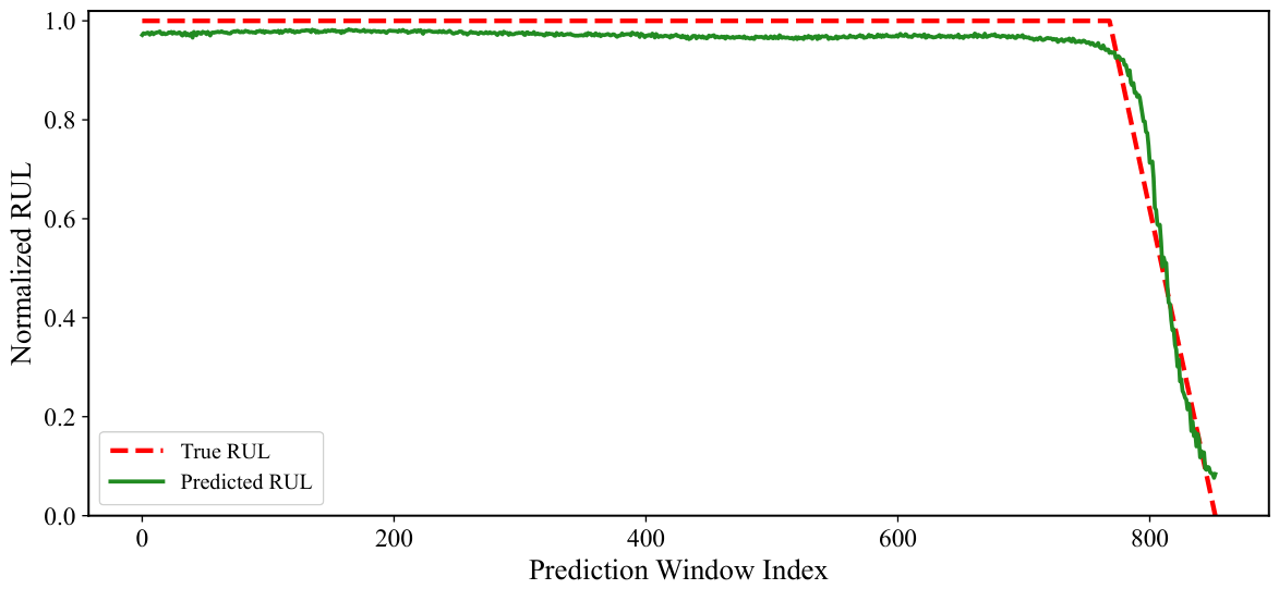
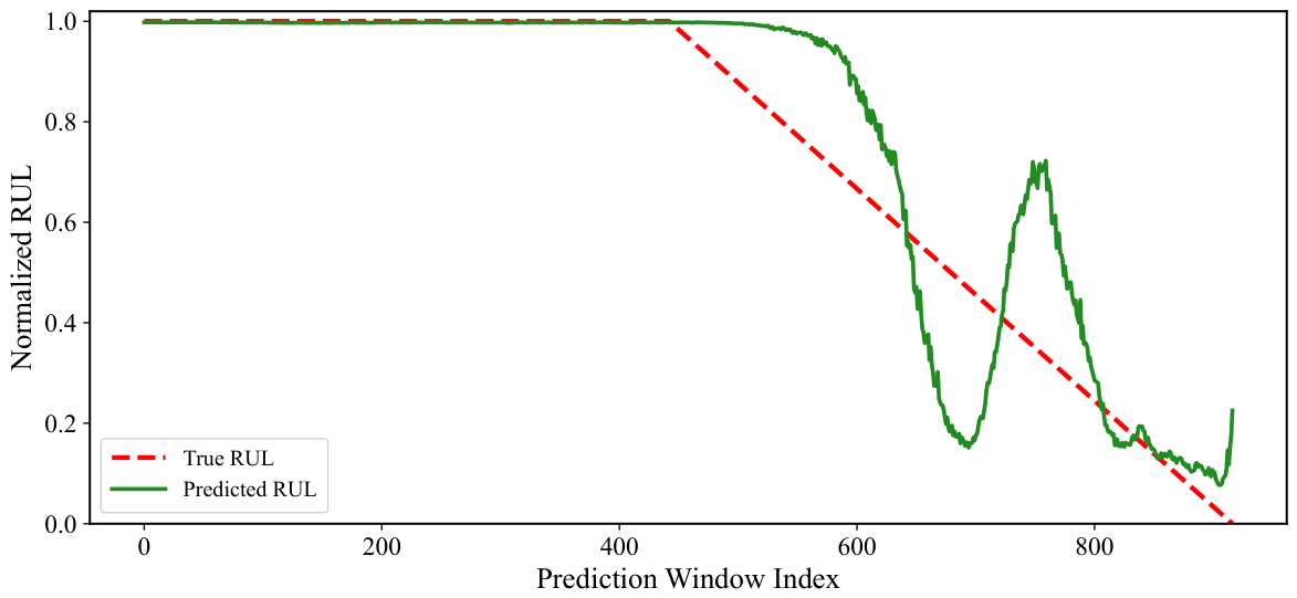
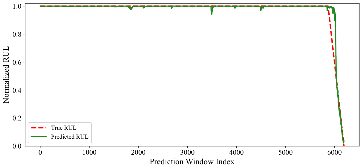
After FPT localization, RUL prediction experiments were further conducted on the test bearings according to the leave-one-bearing-out strategy described in Section 4.3. Figure 11, Figure 12 and Figure 13 present comparison curves between the predicted and ground-truth RUL values for several representative bearings. As can be seen from the figures, the proposed model can generally track the degradation trend of the ground-truth RUL well during the degradation stage.
In addition, Table 9 summarizes the RMSE and MAE values for all test bearings. The results show that the proposed model achieves low prediction errors on the IMS dataset as a whole and maintains relatively stable predictive performance under different degradation patterns. In particular, the errors for most test bearings remain at relatively low levels. By contrast, Bearing2_1 and Bearing3_1 exhibit relatively larger prediction errors than the other test bearings. This may be attributed to the more complex degradation evolution of these two bearings. Specifically, Bearing2_1 shows stronger variability and less regular degradation-feature evolution, whereas Bearing3_1 presents a relatively long quasi-stationary period followed by sharper late-stage deterioration. These characteristics increase the difficulty of accurate degradation characterization and subsequent RUL prediction. Overall, the proposed method still achieves favorable predictive performance on the IMS dataset.
To further verify the effectiveness of the proposed method, comparisons with existing studies were conducted on the IMS dataset, and the results are presented in Table 10. In this table, the lowest value for each evaluation metric is highlighted in bold, whereas the second-lowest value is underlined. Lower RMSE and MAE values indicate better predictive performance. It can be observed that the proposed method exhibits favorable overall predictive performance on the IMS dataset and maintains competitive accuracy compared with the related methods. In addition, the proposed method achieves lower RMSE values than the compared methods for all test bearings included in the comparison, while its MAE values are also lower for most bearings. These results demonstrate that the proposed framework maintains good prediction accuracy and generalization capability under different data distributions. Nevertheless, Bearing2_1 and Bearing3_1 still contribute relatively more to the overall prediction error, indicating that the predictive robustness for bearings with more complex degradation patterns remains to be further improved.

5. Conclusions

To address unreliable degradation-onset identification and inadequate joint modeling of the long-term degradation trend and localized impulsive degradation features in rolling bearing remaining useful life (RUL) prediction, a two-stage framework was proposed, which integrates degradation assessment with DK-Mamba. In the degradation assessment stage, a Mahalanobis-distance-based health indicator was constructed from CEEMDAN-reconstructed signals, and robust degradation-onset identification was achieved through a dual-branch persistent validation mechanism. In the RUL prediction stage, a trend–detail joint modeling framework was developed by integrating multi-scale dynamic decomposition, wavelet-based soft-threshold shrinkage, Mamba-based long-range dependency modeling, JacobiKAN-based nonlinear enhancement, and cross-attention fusion. Experimental results on the PHM2012 and IMS datasets show that the proposed method improves FPT reliability and achieves favorable accuracy and robustness in RUL prediction. Ablation studies further quantify the contribution of each core module. Controlled module-replacement experiments further show that JacobiKAN achieves the lowest average RMSE among the compared nonlinear mapping modules.
However, the proposed framework still has room for improvement in generalization across different datasets and operating conditions. In particular, the relatively larger prediction errors observed for Bearing2_1 and Bearing3_1 in the IMS dataset indicate that model robustness can be further improved for bearings with more complex degradation evolution patterns and cross-domain distribution shifts. Future work will investigate cross-domain transfer learning strategies, such as feature alignment, to reduce distribution discrepancies across datasets and operating conditions, thereby further improving model robustness and cross-condition generalization.

Author Contributions

Conceptualization, Y.Z. and Z.C.; methodology, Y.Z. and Z.C.; software, Y.Z.; validation, Y.Z.; formal analysis, Y.Z.; investigation, Y.Z.; data curation, Y.Z.; writing—original draft preparation, Y.Z.; writing—review and editing, Z.C.; visualization, Y.Z.; supervision, Z.C.; project administration, Z.C. All authors have read and agreed to the published version of the manuscript.

Funding

This research received no external funding.

Institutional Review Board Statement

Not applicable.

Informed Consent Statement

Not applicable.

Data Availability Statement

The raw data used in this study are publicly available from the IEEE PHM 2012 Prognostics Challenge bearing dataset collected on the PRONOSTIA platform and the bearing degradation dataset released by the Intelligent Maintenance Systems Center at the University of Cincinnati. No new experimental data were collected in this study. The processed data supporting the findings of this study are available from the corresponding author upon reasonable request.

Conflicts of Interest

The authors declare no conflicts of interest.

References

  1. Song, L.; Lin, T.; Jin, Y.; Zhao, S.; Li, Y.; Wang, H. Advancements in bearing remaining useful life prediction methods: A comprehensive review. Meas. Sci. Technol. 2024, 35, 092003. [Google Scholar] [CrossRef] [Scilit]
  2. Yan, B.; Ma, X.; Huang, G.; Zhao, Y. Two-stage physics-based Wiener process models for online RUL prediction in field vibration data. Mech. Syst. Signal Process. 2021, 152, 107378. [Google Scholar] [CrossRef] [Scilit]
  3. Yang, F.; Dong, E.; Zhong, Z.; Zhang, W.; Cui, Y.; Ye, J. Remaining useful life prediction of electric drive bearings in new energy vehicles: Based on degradation assessment and spatiotemporal feature fusion. Machines 2025, 13, 914. [Google Scholar] [CrossRef] [Scilit]
  4. Zhao, Y.-S.; Li, P.; Kang, Y.; Zhao, Y.-B. A health indicator enabling both first predicting time detection and remaining useful life prediction: Application to rotating machinery. Measurement 2024, 235, 114994. [Google Scholar] [CrossRef] [Scilit]
  5. Mi, J.; Hou, Y.; He, W.; He, C.; Zhao, H.; Huang, W. A nonparametric cumulative sum-based fault detection method for rolling bearings using high-level extended isolated forest. IEEE Sens. J. 2023, 23, 2443–2455. [Google Scholar] [CrossRef] [Scilit]
  6. Zhang, J.; Zhang, C.; Xu, S.; Liu, G.; Fei, H.; Wu, L. Remaining life prediction of bearings based on improved IF-SCINet. IEEE Access 2024, 12, 19598–19611. [Google Scholar] [CrossRef] [Scilit]
  7. Gugulothu, N.; Vishnu, T.V.; Malhotra, P.; Vig, L.; Agarwal, P.; Shroff, G. Predicting remaining useful life using time series embeddings based on recurrent neural networks. Int. J. Progn. Health Manag. 2018, 9, 1–13. [Google Scholar] [CrossRef] [Scilit]
  8. Kaleli, A.Y.; Unal, A.F.; Ozer, S. Simultaneous prediction of remaining-useful-life and failure-likelihood with GRU-based deep networks for predictive maintenance analysis. In Proceedings of the 2021 44th International Conference on Telecommunications and Signal Processing, Brno, Czech Republic, 26–28 July 2021; pp. 301–304. [Google Scholar]
  9. Yu, Y.; Si, X.; Hu, C.; Zhang, J. A review of recurrent neural networks: LSTM cells and network architectures. Neural Comput. 2019, 31, 1235–1270. [Google Scholar] [CrossRef] [Scilit] [PubMed]
  10. Wang, C.; Jiang, W.; Shi, L.; Zhang, L. Rolling bearing remaining useful life prediction using deep learning based on high-quality representation. Sci. Rep. 2025, 15, 8228. [Google Scholar] [CrossRef] [Scilit] [PubMed]
  11. Jin, X.; Ji, Y.; Li, S.; Lv, K.; Xu, J.; Jiang, H.; Fu, S. Remaining useful life prediction for rolling bearings based on TCN–Transformer networks using vibration signals. Sensors 2025, 25, 3571. [Google Scholar] [CrossRef] [Scilit] [PubMed]
  12. Jin, C.; Li, B.; Yang, Y.; Yuan, X.; Tu, R.; Qiu, L.; Chen, X. Remaining useful life prediction of rolling bearings based on empirical mode decomposition and Transformer Bi-LSTM network. Appl. Sci. 2025, 15, 9529. [Google Scholar] [CrossRef] [Scilit]
  13. Gu, A.; Dao, T. Mamba: Linear-time sequence modeling with selective state spaces. In Proceedings of the First Conference on Language Modeling (COLM 2024), Philadelphia, PA, USA, 7–9 October 2024. [Google Scholar]
  14. Yue, C.; Qin, Y.; Liu, X.; Gu, H.; Sun, S. Data–physics collaborative fusion prediction method for tool remaining useful life based on Mamba state space and physical description. J. Manuf. Syst. 2025, 81, 1–15. [Google Scholar] [CrossRef] [Scilit]
  15. Li, M.; Zhu, L.; Luo, M.; Ke, T. Remaining useful life prediction of airplane engine based on bidirectional Mamba and causal discovery. Sensors 2025, 25, 3429. [Google Scholar] [CrossRef] [Scilit] [PubMed]
  16. Liu, F.; Liu, S.; Chai, Y.; Zhu, Y. Enhanced Mamba model with multi-head attention mechanism and learnable scaling parameters for remaining useful life prediction. Sci. Rep. 2025, 15, 7178. [Google Scholar] [CrossRef] [Scilit] [PubMed]
  17. Zhang, G.; Lei, C.; Zhou, J.; Hao, D.; Li, X.; Li, M.; Feng, R. Remaining useful life prediction method for rolling bearings based on Mamba-SDP. J. Mech. Sci. Technol. 2025, 39, 7473–7488. [Google Scholar] [CrossRef] [Scilit]
  18. Liu, Z.; Wang, Y.; Vaidya, S.; Ruehle, F.; Halverson, J.; Soljačić, M.; Hou, T.Y.; Tegmark, M. KAN: Kolmogorov–Arnold networks. In Proceedings of the Thirteenth International Conference on Learning Representations (ICLR 2025), Singapore, 24–28 April 2025. [Google Scholar]
  19. Aghaei, A.A. fKAN: Fractional Kolmogorov–Arnold networks with trainable Jacobi basis functions. Neurocomputing 2025, 623, 129414. [Google Scholar] [CrossRef] [Scilit]
  20. Torres, M.E.; Colominas, M.A.; Schlotthauer, G.; Flandrin, P. A complete ensemble empirical mode decomposition with adaptive noise. In Proceedings of the 2011 IEEE International Conference on Acoustics, Speech and Signal Processing, Prague, Czech Republic, 22–27 May 2011; pp. 4144–4147. [Google Scholar]
  21. De Maesschalck, R.; Jouan-Rimbaud, D.; Massart, D.L. The Mahalanobis distance. Chemom. Intell. Lab. Syst. 2000, 50, 1–18. [Google Scholar] [CrossRef] [Scilit]
  22. Peng, H.; Long, F.; Ding, C. Feature selection based on mutual information: Criteria of max-dependency, max-relevance, and min-redundancy. IEEE Trans. Pattern Anal. Mach. Intell. 2005, 27, 1226–1238. [Google Scholar] [CrossRef] [Scilit] [PubMed]
  23. Whitney, A.W. A direct method of nonparametric measurement selection. IEEE Trans. Comput. 1971, C-20, 1100–1103. [Google Scholar] [CrossRef] [Scilit]
  24. Gu, A.; Goel, K.; Ré, C. Efficiently modeling long sequences with structured state spaces. In Proceedings of the Tenth International Conference on Learning Representations (ICLR 2022), Virtual, 25–29 April 2022. [Google Scholar]
  25. El Afia, H.; Ohamouddou, S.; Chiheb, R.; El Afia, A. Dynamic graph CNN with Jacobi Kolmogorov–Arnold networks for 3D classification of point sets. arXiv 2025, arXiv:2506.06296. [Google Scholar]
  26. Nectoux, P.; Gouriveau, R.; Medjaher, K.; Ramasso, E.; Chebel-Morello, B.; Zerhouni, N.; Varnier, C. PRONOSTIA: An experimental platform for bearings accelerated degradation tests. In Proceedings of the IEEE International Conference on Prognostics and Health Management, Denver, CO, USA, 18–21 June 2012; pp. 1–8. [Google Scholar]
  27. An, X.; Zhang, C.; Liu, C.; Zhao, W. An enhanced approach for remaining useful life prediction of bearings using incomplete lifecycle data. IEEE Access 2025, 13, 53305–53320. [Google Scholar] [CrossRef] [Scilit]
  28. Luo, X.; Wang, M. Bearing lifespan reliability prediction method based on multiscale feature extraction and dual attention mechanism. Appl. Sci. 2025, 15, 3662. [Google Scholar] [CrossRef] [Scilit]
  29. Wang, C.; Jiang, W.; Yang, X.; Zhang, S. RUL prediction of rolling bearings based on a DCAE and CNN. Appl. Sci. 2021, 11, 11516. [Google Scholar] [CrossRef] [Scilit]
  30. Qiu, H.; Lee, J.; Lin, J.; Yu, G. Wavelet filter-based weak signature detection method and its application on rolling element bearing prognostics. J. Sound Vib. 2006, 289, 1066–1090. [Google Scholar] [CrossRef] [Scilit]
  31. Ding, G.; Wang, W.; Zhao, J. Prediction of remaining useful life of rolling bearing based on fractal dimension and convolutional neural network. Meas. Control 2022, 55, 79–93. [Google Scholar] [CrossRef] [Scilit]
  32. Li, J.; Ding, W.; Mao, W.; Zhang, J.; Meng, Z.; Tong, K. Causal dilated convolution-based residual DenseNet with channel attention for RUL prediction of rolling bearings. Measurement 2024, 235, 115012. [Google Scholar] [CrossRef] [Scilit]
Figure 1. Flowchart of FPT identification based on CEEMDAN and the health indicator.
Machines 14 00836 g001
Figure 2. Overall architecture of the proposed DK-Mamba framework.
Machines 14 00836 g002
Figure 3. Structure of the MSDD trend–detail decomposition module.
Machines 14 00836 g003
Figure 4. Architecture of the detail encoder, JacobiKAN, and Mamba modules.
Machines 14 00836 g004
Figure 5. Selected feature curves.
Machines 14 00836 g005
Figure 6. Feature selection results and redundancy analysis based on mRMR: (a) feature relevance ranking based on mutual information with RUL; (b) feature redundancy matrix based on pairwise mutual information.
Machines 14 00836 g006aMachines 14 00836 g006b
Figure 7. Reference-free quantitative consistency evaluation of FPT localization for Bearing1_3: (a) RMS and envelope energy used for HI construction; (b) HI curve and FPTs identified by different methods; (c) MAD-normalized deviations of the independent validation features; and (d) quantitative comparison of the detected FPTs.
Machines 14 00836 g007
Figure 8. RUL prediction results for Bearing1_3 in the PHM2012 dataset.
Machines 14 00836 g008
Figure 9. Global and locally enlarged RUL prediction results for Bearing1_7 in the PHM2012 dataset.
Machines 14 00836 g009
Figure 10. RUL prediction results for Bearing3_2 in the PHM2012 dataset.
Machines 14 00836 g010
Figure 11. RUL prediction results for Bearing2_1 in the IMS dataset.
Machines 14 00836 g011
Figure 12. RUL prediction results for Bearing2_3 in the IMS dataset.
Machines 14 00836 g012
Figure 13. RUL prediction results for Bearing3_2 in the IMS dataset.
Machines 14 00836 g013
Table 1. Candidate features.
CategoryFeaturesCategoryFeatures
Time DomainMeanTime DomainRoot_amplitude
Variancep-norm Crest Factor ( P = 1.9 )
SkewnessMargin factor
KurtosisFrequencySpectral_flatness
Peak_vibrationEnergy_ratio
Rms_vibrationComplexityEntropy
Peak_factorFractal_Dimension
Pulse_factor
Table 2. Quantitative comparison of FPT localization methods for Bearing1_3.
MethodFPTBaseline
Shift
Buffered
Separation
Support
Rate
Persistence
Ratio
Relapse
Ratio
RMS 3 σ 11012.1041.0220.400.7970.203
Kurtosis 3 σ 6020.4480.4760.000.2030.797
HI single threshold6030.4550.4950.000.1960.804
Dual branch without validation13195.3732.5910.600.9930.007
DPV-FPT13437.5784.0020.601.0000.000
Table 3. Summary of FPT localization results for all bearings in the PHM2012 dataset.
BearingFPTBearingFPT
Bearing1-11388Bearing1-62418
Bearing1-2827Bearing1-72172
Bearing1-31343Bearing3-1494
Bearing1-41085Bearing3-21602
Bearing1-52429Bearing3-3322
Table 4. RUL prediction errors of the test bearings in the PHM2012 dataset.
MetricBearing1_3Bearing1_5Bearing1_6Bearing1_7Bearing3_2
RMSE0.01700.03600.04000.00690.0372
MAE0.01020.01260.00760.00320.0166
Table 5. Performance comparison with related methods on the PHM2012 dataset.
ModelMetricBearing1_3Bearing1_5Bearing1_7Average
Proposed MethodRMSE0.01700.03600.00690.0200
MAE0.01020.01260.00320.0087
Ref. [12]RMSE0.04540.06570.0556
MAE0.03790.05420.0461
Ref. [27]RMSE0.04700.05800.06300.0560
MAE0.03800.04600.05000.0447
Ref. [28]RMSE0.10500.08400.05900.0827
MAE0.08900.07200.04800.0697
Ref. [29]RMSE0.05400.06800.0610
MAE0.03700.10300.0700
Table 6. Results of the module ablation experiments.
ModelMetricBearing1_3Bearing1_7Bearing3_2Average
Proposed MethodRMSE0.01700.00690.03720.0204
MAE0.01020.00320.01660.0100
w/o MSDDRMSE0.03460.06620.08370.0615
MAE0.01750.02480.02100.0211
w/o JacobiKANRMSE0.01980.01790.05750.0317
MAE0.01250.00380.01340.0099
w/o WaveletRMSE0.01770.01370.04850.0266
MAE0.00960.00470.02160.0120
Table 7. Comparison of different nonlinear mapping modules in the high-frequency detail branch.
ModuleBearing1_3Bearing1_7Bearing3_2Average
MAERMSEMAERMSEMAERMSEMAERMSE
KAN0.02060.03670.00950.01500.01530.04690.01510.0329
ChebyKAN0.01320.02310.00530.01090.01660.03720.01170.0237
MLP0.01290.02080.00620.01090.01040.05590.00980.0333
JacobiKAN0.01020.01700.00320.00690.01660.03720.01000.0204
Table 8. FPT localization results for all bearings in the IMS dataset.
BearingFPTBearingFPT
Bearing2-1510Bearing3-16144
Bearing2-2874Bearing3-26000
Bearing2-3880Bearing3-36050
Bearing2-4864Bearing3-46012
Table 9. RUL prediction errors for all bearings in the IMS dataset.
BearingRMSEMAEBearingRMSEMAE
Bearing2_10.06110.0364Bearing3_10.06960.0144
Bearing2_20.03170.0197Bearing3_20.03860.0072
Bearing2_30.03340.0308Bearing3_30.04450.0077
Bearing2_40.04760.0358Bearing3_40.04170.0073
Table 10. Performance comparison of different methods on the IMS dataset.
ModelMetricBearing2_1Bearing2_2Bearing2_3Bearing2_4Average
OursRMSE0.06110.03170.03340.04760.0435
MAE0.03640.01970.03080.03580.0307
Ref. [31]RMSE0.06910.11800.10710.08220.0941
MAE0.04620.09800.08680.06770.0747
Ref. [32]RMSE0.06120.05280.03420.05920.0519
MAE0.04700.04140.02670.04560.0402
Disclaimer/Publisher’s Note: The statements, opinions and data contained in all publications are solely those of the individual author(s) and contributor(s) and not of MDPI and/or the editor(s). MDPI and/or the editor(s) disclaim responsibility for any injury to people or property resulting from any ideas, methods, instructions or products referred to in the content.