1. Introduction
Tool path planning serves as a fundamental technology in the Computer-Aided Manufacturing (CAM) stage, which is pivotal to the modern machining process. Tool path planning comprises three main stages [
1]: Roughing, Semi-Finishing, and Finishing, each fulfilling a specific function and ultimately guaranteeing that the workpiece achieves the required shape and surface quality. The process begins with the roughing stage, which performs high-efficiency volume removal to approximate the designed shape. Semi-Finishing then machines the surface to prepare it for finishing. The process concludes with the Finishing stage, which achieves the final shape and surface quality as specified in the design.
Within the finishing stage, a sub-process known as corner cleaning is performed to remove residual material from previous operations, such as residual material arising from geometric constraints between the tool and workpiece [
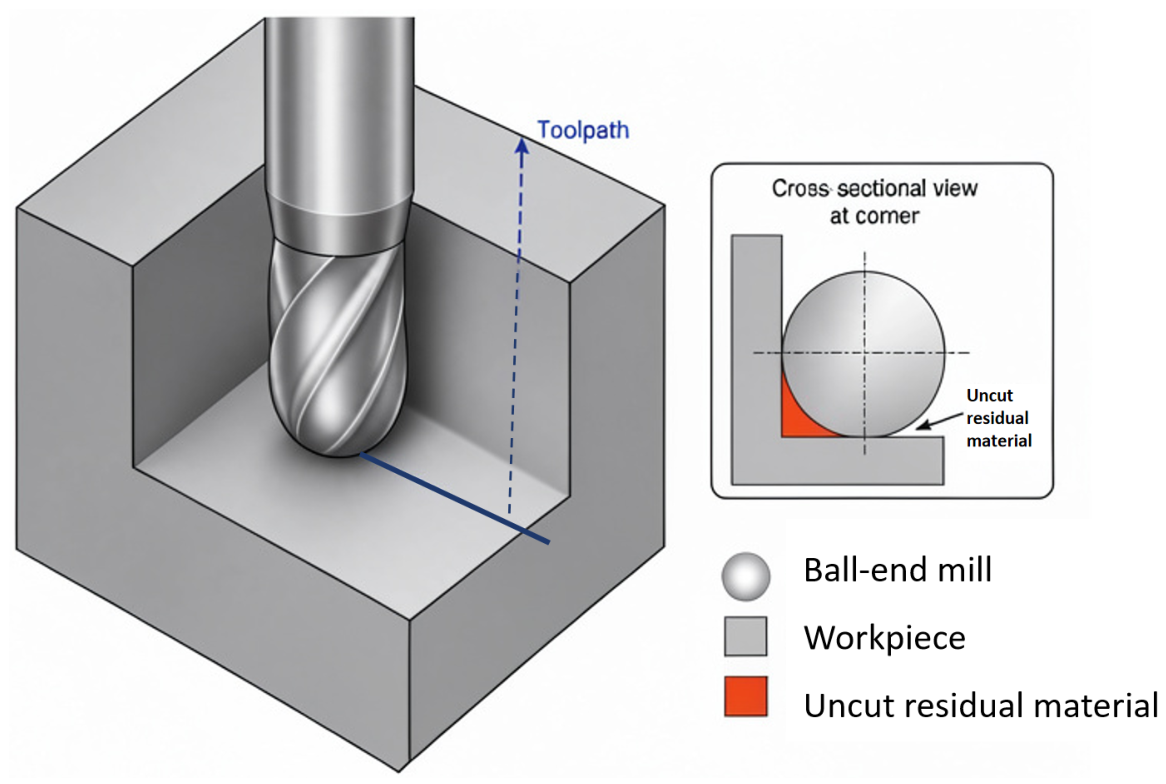
2]. For instance, a ball-end mill’s spherical geometry prevents complete material removal in sharp corners, leaving uncut material, as shown in
Figure 1; similarly, any tool whose diameter exceeds the groove width cannot penetrate into the groove, thereby leaving residual material. In multi-axis machining, improper tool orientation may cause tool–workpiece collision interference or fail to reach residual material in corners. As an essential step in finishing, corner cleaning addresses these residual material issues to ensure the final workpiece conforms to all design specifications.
Although corner cleaning machining plays a vital role in the machining process, this procedure has lacked support from new fundamental theories in recent years. First, academia has paid insufficient attention to corner cleaning machining, and dedicated research literature on this topic is rather limited. Furthermore, commercial CAM software typically relies on descriptive definitions, such as generating tool paths for unprocessed sharp corners and residual material zones, yet such descriptions lack innovative theoretical representation and modeling frameworks. In practice, due to the complex and variable geometric characteristics of corner cleaning areas, their identification still depends heavily on manual observation and inspection, falling short of full automation. Establishing rigorous mathematical definitions and a solid theoretical foundation is therefore imperative.
A second challenge concerns tool path generation. The drive curve offset strategy, while being the predominant industry approach for ensuring path uniformity in corner cleaning, relies on manual drive curve selection in commercial CAM software and lacks theoretical optimization for efficiency [
3]. Refining this algorithm and establishing its theoretical basis are therefore key to advancing automation.
To address these current gaps, this manuscript presents a comprehensive solution for corner cleaning. The contributions of this work are threefold: a rigorous mathematical framework for defining corner cleaning regions, a robust method for drive curve generation and offsetting, and a complete tool path planning strategy. These components collectively offer the following advantages over the state of the art:
Theoretical Completeness: Starting from the construction of rigorous mathematical definitions, the proposed method establishes a comprehensive theoretical framework for corner cleaning, thereby ensuring theoretical integrity.
Application Robustness: The proposed method constructs drive curves based on point clouds, thus maintaining compatibility with diverse CAD representations. Experimental results demonstrate that the proposed approach achieves superior robustness compared to the widely used commercial CAM software PowerMill 2024 (PM24).
Path Smoothness: The proposed self-intersection removal and trimming algorithms enable the generation of self-intersection-free, smooth, and continuous tool paths from the offset curves of the drive curve.
This paper is structured as follows:
Section 2 reviews related work in path planning of corner cleaning.
Section 3 presents our methodology, including the mathematical framework (
Section 3.1), tool radius decision method (
Section 3.2), enhanced PCA-based drive curve generation (
Section 3.3), and the complete path smoothing strategy (
Section 3.4). In
Section 4, some experiments are conducted to illustrate and clarify our method. The comparison in case study with commercial software proves the superiority of our method. And the paper concludes in
Section 5.
2. Related Work
This work addresses tool path planning for corner cleaning in 3-axis machining, focusing specifically on cutter contact (CC) point planning. Regarding tool selection, due to the surface quality requirements in the finishing stage, this paper adopts ball-end mills for both corner cleaning phase and the preceding Finishing process. Within this technical scope, this section reviews existing related methodologies.
As a sub-stage of the finishing process, corner cleaning can theoretically adopt any existing tool path planning method developed for the Finishing stage. This section begins with a concise review of existing finishing tool path planning methods and analyzes their inherent limitations when applied to corner cleaning scenarios. Subsequently, the drive-curve offset strategy for corner cleaning is introduced, along with a discussion of its practical constraints. Finally, the remaining theoretical gaps that the proposed work aims to address are identified.
2.1. Path Planning Methods for Finishing Stage
Tool path planning approaches for the finishing process can be primarily categorized into two groups: geometry-driven methods and mathematical model-based methods.
Developed as early-stage approaches, geometry-driven methods utilize geometric features and discrete computing to accomplish machining area coverage. These approaches include iso-parametric methods [
4,
5,
6,
7] that directly employ surface iso-parametric curves as tool paths, iso-planar methods [
8,
9,
10,
11,
12] that generate paths from intersections between parallel planes and the surface, and iso-scallop methods [
13,
14,
15,
16,
17,
18,
19] that offset an initial path while maintaining uniform scallop height to achieve complete surface coverage. Of these approaches, iso-parametric and iso-planar methods fail to maintain uniform scallop, while the iso-scallop method is prone to robustness issues caused by the self-intersection of offset curves. Furthermore, its path quality heavily depends on the selection of the initial tool path.
Mathematical model-based methods transform the path planning problem into solving equations or optimization problems under geometric and machining constraints, aiming to produce smooth and short paths over complex surfaces. This category mainly consists of vector field methods [
20,
21,
22,
23,
24,
25,
26,
27,
28,
29], which derive locally optimal directions from surface geometry to construct guiding vector fields, and heat diffusion methods [
30,
31,
32,
33] that simulate thermal propagation on surfaces to generate tool paths that approximate geodesic offsets. While both methodologies can achieve high path quality, their effectiveness relies on explicit CAD representations and mathematical computation. However, in corner cleaning scenarios, the target machining areas typically span multiple surface patches with irregular boundaries, and thus cannot fully inherit the original CAD representation. Consequently, applying these approaches directly to corner cleaning path planning lacks robustness.
2.2. Drive Curve Offset Method
The drive curve offset strategy is an application of the iso-scallop method in corner cleaning scenarios, where the drive curve corresponds to the initial path in the iso-scallop framework. This approach thus preserves the iso-scallop method’s ability to maintain uniform scallop while inheriting its characteristic limitations, including dependence on initial curve selection and potential self-intersection of the offset paths. These challenges are reflected in both academic research and industrial practice.
Theoretically, current research on the iso-scallop method lacks specialized development for corner cleaning applications. When applied to the specialized machining regions in corner cleaning, the method needs to overcome challenges posed by incomplete or non-connected CAD representations while establishing appropriate optimization objectives and computational approaches for drive curve (initial path) generation. Practically in commercial CAM software, drive curves are either manually defined by users or automatically provided by the software. However, in both cases, the theoretical foundation underlying the generation of drive curves has not been updated for a long time. Furthermore, to maintain path smoothness, the self-intersection issue in offset curves must be properly addressed during the offsetting process.
2.3. Research Gaps and Our Contributions
In summary, while mathematical model-based methods are generally unsuitable for corner cleaning due to their dependency on CAD representations, and both iso-parametric and iso-planar methods lack control of uniform scallop, the iso-scallop method consequently emerges as the preferred approach. In this context, it is generally known as the drive curve offset strategy. Nevertheless, this method still faces theoretical and practical challenges that limit its effectiveness and robustness.
To address these challenges, this manuscript establishes a comprehensive mathematical framework specifically for corner cleaning, including formal definitions of machining regions and optimized tool selection criteria. Based on this framework, we propose a complete pipeline comprising an automated drive curve generation method, robust offset operations with self-intersection handling, and smooth path connection. The following section details the proposed method and demonstrates how it systematically bridges the research gaps.
3. Methodology
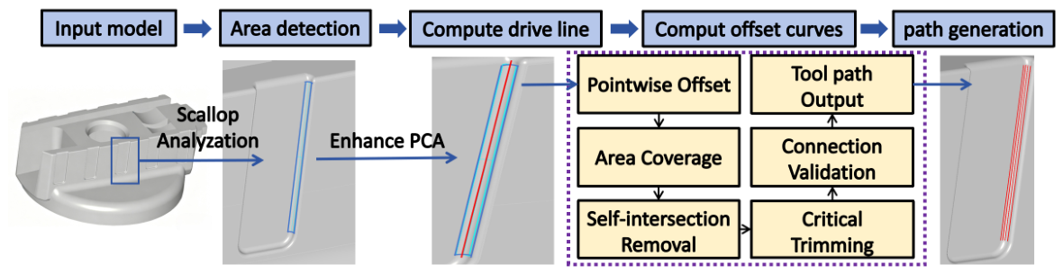
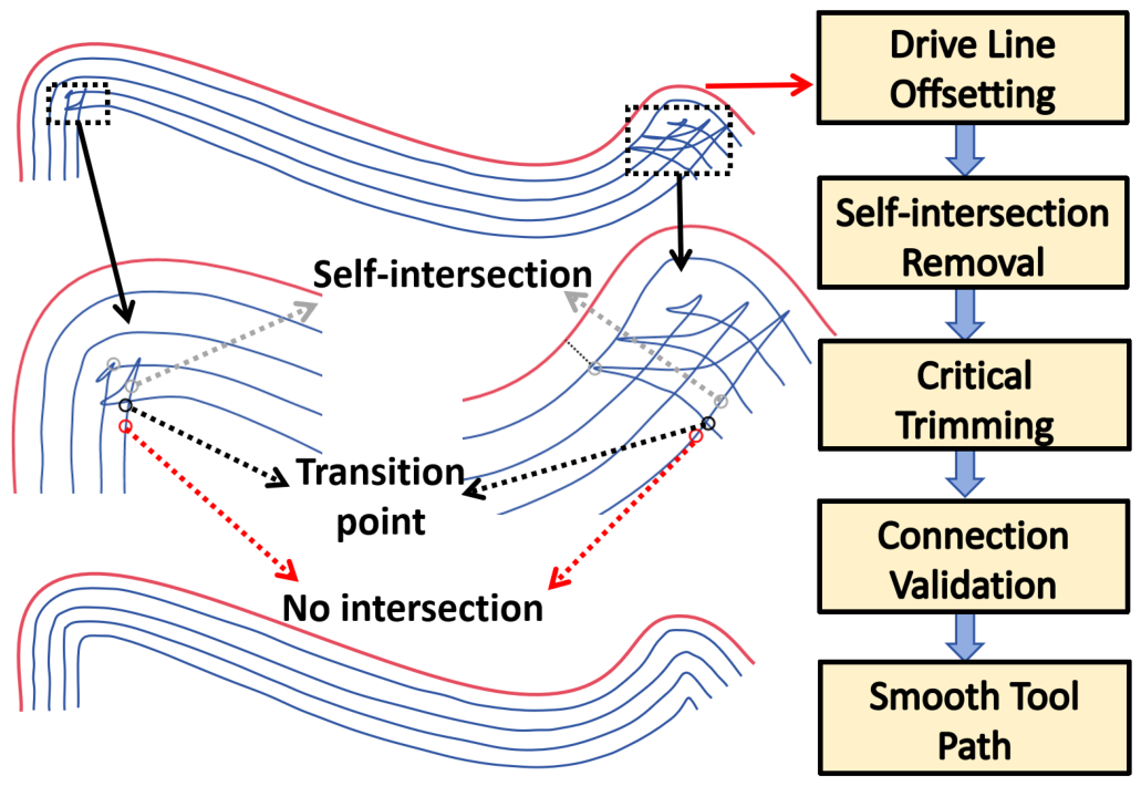
This section introduces the theoretical framework of the proposed corner cleaning method, comprising four key components: the mathematical definitions of target regions, a tool radius selection criterion, a drive curve construction methodology, and a complete tool path generation algorithm that ensures path continuity and smoothness. The complete workflow is illustrated in
Figure 2.
3.1. Mathematical Definitions
The target machining areas in corner cleaning are defined as corner cleaning regions. This subsection establishes a complete mathematical characterization of these regions, extending beyond the descriptive definitions commonly adopted in industrial CAM software. The corner cleaning regions are determined by the workpiece surface, the previous machining tool paths, the previous cutting tool, and the given scallop constraint, as specified by the following inputs:
Workpiece surface ;
Previous machining paths set , where t denotes parameter for continuous curves or discrete index for G01 points;
Previous tool radius ;
Scallop constraint h.
For each in the previous machining tool paths, we declare the following elements for subsequent calculations:
The outward normal vector ;
The tangent vector of the tool path ;
The offset direction: .
where × denotes the cross product in .
For each point in the machining path
and its corresponding offset direction
(assume that the tool paths generated in the prior Finishing operation before corner cleaning is a iso-scallop height paths), the path interval denoted as
satisfying scallop constraint is determined by the following formula:
in which
represents the radius of curvature of the workpiece surface along the path offset direction
.
Considering that corner cleaning regions refer to areas that still violate the scallop constraint due to geometric constraints between the tool and workpiece during the previous machining step, the following definitions are introduced:
Definition 1 (Sweep Curve).
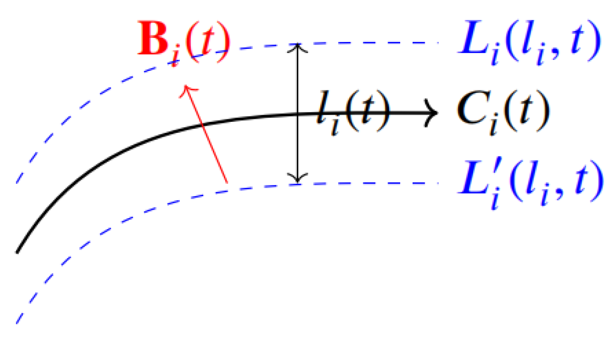
For a machining path with computed path interval , the corresponding residual height curves are two curves on the workpiece surface satisfying at every parameter t: As shown in
Figure 3, after machining solely along the path
on the workpiece surface, the sweep curve on surfaces with moderate curvature variation generally lies midway between adjacent tool paths. This sweep curve approximately demarcates the boundary where residual height satisfies the scallop constraints. The region between
and
satisfies the specified scallop constraint
h. Accordingly, the regions on the workpiece surface are categorized based on residual height distribution after completing all previous machining operations:
Definition 2 (Local Sweep Region).
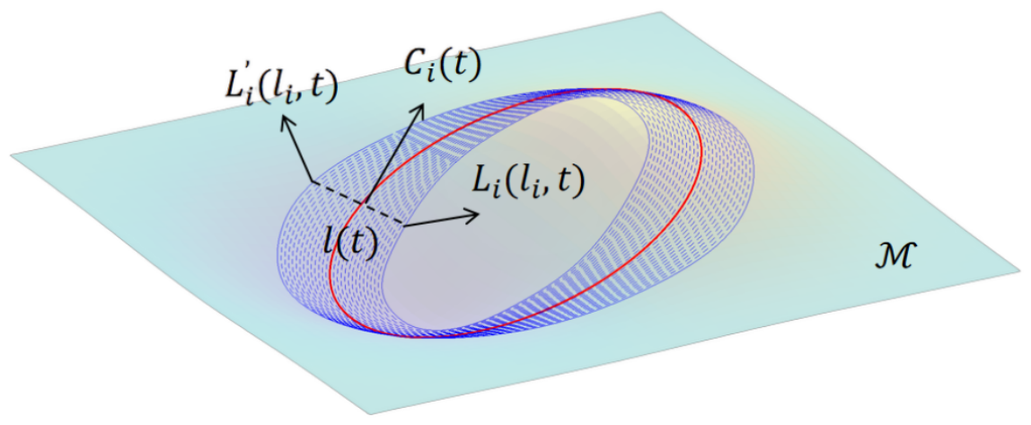
For each machining path , the corresponding local sweep region is defined as:which represents the surface region swept by the sweep curves as the constraint parameter α varies from 0 to h, as illustrated in Figure 4. Definition 3 (Complete Sweep Region).
The complete sweep region is defined as the union of all local sweep regions:which represents all surface regions that satisfying the scallop constraints after previous machining operations. Definition 4 (Corner Cleaning Region).
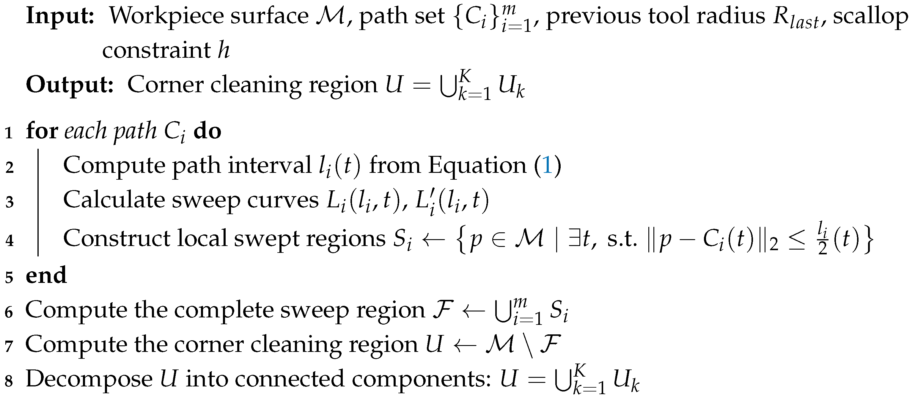
The corner cleaning region is defined as the boolean difference of the workpiece surface and the complete sweep region:representing all surface regions failing to satisfy the scallop constraints after the previous machining operations. The above establishes the definitions and notational conventions for corner cleaning regions and related concepts. Given the workpiece surface geometry along with machining parameters and tool paths from the preceding operations, path intervals, sweep curves, and the local swept regions associated with each path are systematically computed. These are subsequently integrated to form the complete swept region, from which the target corner cleaning area is derived. The detailed computational procedure is presented in Algorithm 1.
| Algorithm 1: Detection of Corner Regions to Be Cleaned Up |
 |
3.2. Tool Radius Decision
Once the corner cleaning region is identified, selecting an appropriate ball-end mill radius becomes crucial for effective residual material removal. Improper tool selection can lead to incomplete machining of target areas. This subsection establishes theoretical constraints for tool radius determination.
Let
denote the minimum principal curvature of the corner cleaning region. Then, the tool radius
should satisfy the following inequality:
Which ensures the tool tip can fully access concave regions without causing over-cutting of the workpiece surface. In practical applications, a safety factor
is introduced to decide the tool radius:
To maintain compatibility with CAD representations, the point cloud
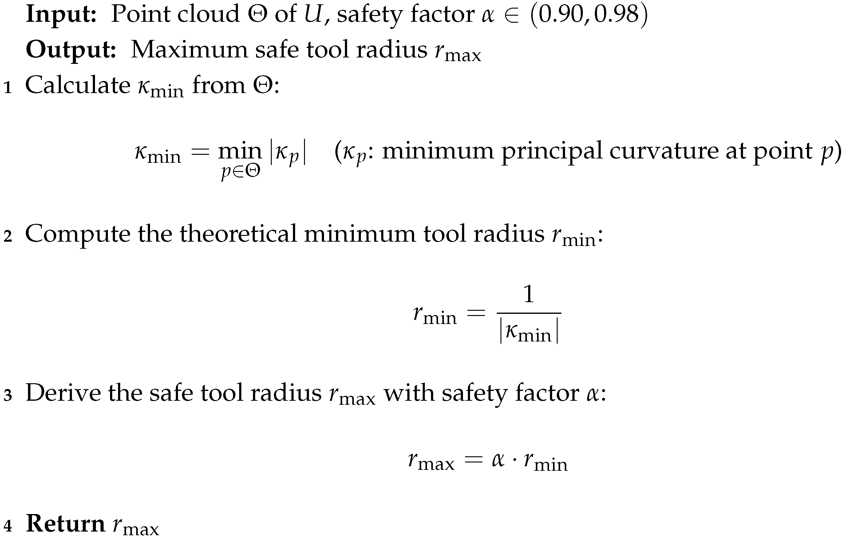
generated from the corner cleaning region is processed (any workpiece model in CAD format can be converted to a point cloud via sampling). The absolute values of minimum principal curvatures are computed for all points [
34], from which the global minimum is determined to establish the safe tool radius. The detailed computational procedure for tool radius constraint is presented in Algorithm 2.
| Algorithm 2: Tool Radius Calculation |
 |
3.3. Drive Curve Construction
Following the determination of corner cleaning regions and tool radius, tool paths are generated using the drive curve offset method. The process begins with constructing a drive curve , followed by offsetting this initial curve within the corner cleaning region to achieve complete area coverage. This subsection provides a detailed explanation of the drive curve construction methodology which directly determines the sweep efficiency of the subsequent offset tool paths.
3.3.1. Direction of Drive Curve
For the input corner cleaning region, the direction of the drive curve is first determined based on the Principal Component Analysis (PCA) method. To ensure compatibility with CAD representations, the region is discretized into a point cloud
, from which the optimal drive curve direction is derived with its corresponding maximum strip width vector field [
21].
Given the point cloud and its associated maximum strip width vector field , let represent the average direction of this vector field. The principal direction is computed using an enhanced PCA approach that integrates two complementary sources of information: the vector field provides optimal strip width guidance, while standard PCA identifies the direction of maximum data variance, which enables the drive curve to achieve greater length. This hybrid strategy enhances the sweeping efficiency of the resulting drive curve. The combined optimization objectives are therefore formulated as follows:
To integrate these two objectives, we formulate the optimization problem through a linear combination of both criteria:
where
is the covariance matrix and
denotes the mean point of the point cloud,
is the balancing weight coefficient.The weighting coefficient
governs the balance between the two objectives in the following pattern:
As , the method converges to standard PCA;
As , the drive curve direction converges to .
For practical implementation, the weighting coefficient is typically set within the range in our method.
The optimization problem can be reformulated as an eigenvalue problem for a new defined matrix
:
And
possesses the following properties:
As a symmetric positive semi-definite matrix,
has efficient solution through standard eigen-decomposition:
Sorting the computed eigenvalues in descending order
, the optimal principal direction of the enhanced PCA corresponds to the eigenvector
associated with
. This direction is selected as the direction for the drive curve.
As shown in
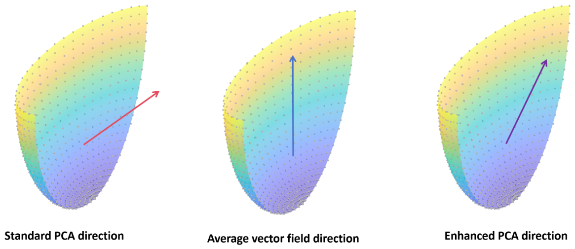
Figure 5, by integrating the directional information from the vector field through the enhanced PCA method, the drive curve direction achieves simultaneous optimization of both strip width and data distribution variance, resulting in higher sweeping efficiency of the drive curve: tool paths following the standard PCA direction exhibit lower strip width utilization, those aligned with the average vector field direction require a greater number of paths, while the enhanced PCA direction achieves a balance between these factors. The complete algorithm implementation is presented in Algorithm 3.
| Algorithm 3: Drive Curve Direction Calculation |
 |
At the end of this subsection, it is demonstrated that the eigenvector
corresponding to the maximum eigenvalue is the solution to optimization problem (
4), i.e., the following theorem holds:
Theorem 1. Let be the eigenvector corresponding to the largest eigenvalue of matrix . Then is the solution to optimization problem (4). Proof. First, since
is a symmetric positive semi-definite matrix,
exists. Let its corresponding eigenvalue be
. We apply the method of Lagrange multipliers by imposing the constraint
and constructing the Lagrangian:
Setting the gradient of
to zero:
Rearranging the expression yields the eigenvalue equation:
Thus,
is an extreme point of the function
. Consider the Hessian matrix:
And at the eigenvector
, we have:
Moreover, since
is the largest eigenvalue of
and
is symmetric, the eigenvalues of
are the differences between the eigenvalues of
and
. Therefore, the symmetric matrix
is negative semi-definite, so
is a maximum point.
In conclusion, by the method of Lagrange multipliers, Theorem 1 holds. □
3.3.2. Generation of Drive Curve
In this subsection, the drive curve is generated using , the computed direction , and the surface average normal through the following steps:
Project along to determine the baseline segment,
Extend segment endpoints to improve robustness,
Construct extended planar regions using ,
Obtain the drive curve as the intersection between plane and the workpiece surface.
To maintain compatibility with CAD formats, the drive curve is uniformly represented using discrete points for all input models. The number of discrete points N can be determined based on the maximum and minimum principal curvatures of the workpiece surface and the given chord error tolerance.
Let
be the maximum absolute value of the principal curvatures of the workpiece surface, where
denotes the chord error tolerance. For a sampling interval
d and the corresponding directional normal curvature
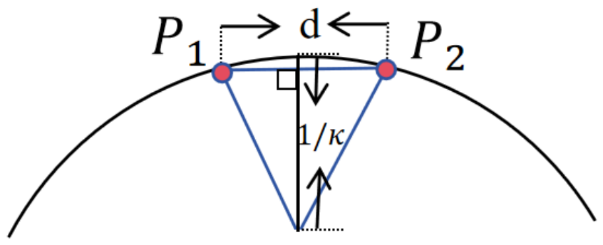
, as shown in
Figure 6, the induced chord error is:
For a given maximum allowable chord error
, the maximum sampling interval is:
This indicates that the maximum sampling interval decreases monotonically with the absolute value of the normal curvature. Therefore, using
to compute the sampling interval satisfies the chord error tolerance requirement. Let the length of the drive curve be
L. Then, the total number of sampling points is calculated as:
A straight line along
passing through the centroid of
is constructed, the point cloud is projected onto this line, and the minimum and maximum projection coordinates are determined based on the farthest projection points at both ends of the line. Then, according to a specified extension coefficient, the extended projection interval on the line is determined. Using Equation (
10), the number of sampling points is computed to obtain a discrete point sequence on the projection line, which is then projected onto the corner cleaning region along
to form the drive curve. The detailed procedure for constructing the drive curve is presented in Algorithm 4.
In the algorithm, the projection coordinates
and
represent the theoretical lower and upper bounds of the projection axis, which would encompass the projection range of the entire corner cleaning region. However, to enhance algorithmic robustness, an extension coefficient
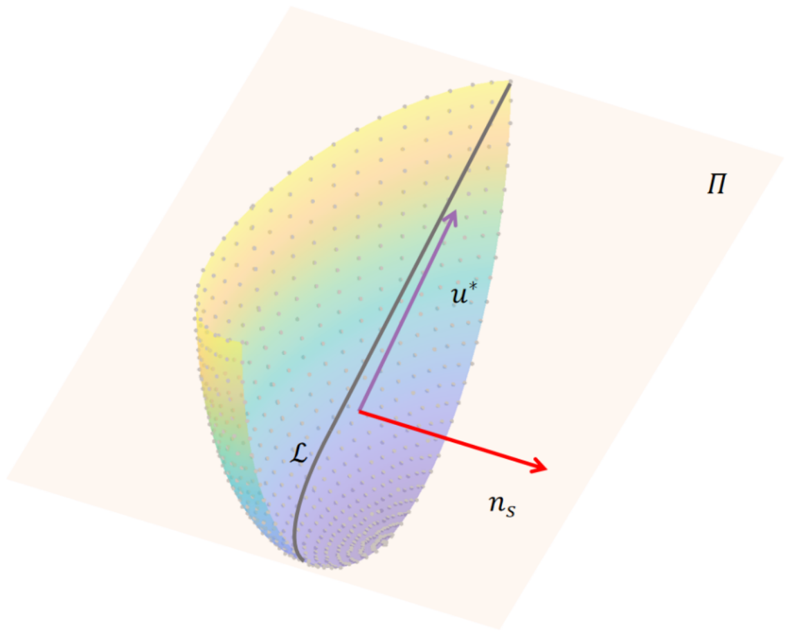
is introduced to extend the projection range at both ends. This extended range, combined with the surface average normal, defines a plane. The intersection curve between this plane and the corner cleaning region constitutes the drive curve, as illustrated in
Figure 7.
| Algorithm 4: Drive Curve Generation |
 |
This subsection presents the drive curve generation process, which begins with computing the direction via the enhanced PCA method. A reference straight line is then discretely constructed through the point cloud centroid and subsequently projected onto the corner cleaning region to form the final drive curve. The following subsection describes how drive curve offsets are utilized to cover the corner cleaning region, eliminate self-intersections in offset curves, and ultimately generate smooth tool paths.
3.4. Path Generation
3.4.1. Generation of Offset Curves
When offsetting the drive curve, it is necessary to account for whether the curve forms a closed loop. Given a discrete drive curve point set
, its closure property is first determined via an endpoint distance threshold:
where
is a parameter typically set to 1% of the tool radius. For each point
, compute the tangent vector
using central difference strategy:
Define the current tangent vector
, then normalize:
Given surface outward normal
at
, compute two offset directions via right-hand rule:
To maintain scallop uniformity, the offset distance is computed by Equation (
1). The offset curves are then iteratively generated by applying directional offsets to the new curve until all points of the curve lie within the complete sweep region. This procedure is applied separately to both sides of the drive curve. The detailed procedure is presented in Algorithm 5.
This algorithm generates bidirectional offsets from the drive curve to achieve complete coverage of the corner cleaning region. The resulting offset curves are subsequently smoothed to ensure path continuity before being output as the final tool paths for corner cleaning.
3.4.2. Self-Intersection Removal with Trimming
This subsection introduces a detection and trimming strategy for generating intersection-free tool paths. During the offset of the drive curve, self-intersection may occur in the offset curve when the original curve exhibits curvature variations or the offset distance exceeds a critical value, leading to geometrically invalid tool paths. For smooth curves, this phenomenon arises when the offset distance
d exceeds the local radius of curvature
R, satisfying the condition:
where
denotes the curvature at the curve parameter
s, and
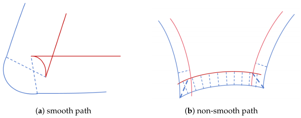
represents the minimum curvature radius of the curve, as illustrated in
Figure 8a. For non-smooth curves or polylines, self-intersection can also emerge at locations with local sharp angles, as shown in
Figure 8b. Both types of self-intersection must be handled during tool path generation from curve offsets.
| Algorithm 5: Offset Curve Generation |
 |
First thing to do is the detection of self-intersection. For the
k-th offset curve
, define the self-intersection indicator function [
35]:
where
is the average path interval derived from the geodesic curve between
and
, computed via its average curvature
and scallop constraint
h (using Equation (
1)).
Each point
on the
k-th offset curve is obtained by offsetting a seed point on the drive curve
k times. The geodesic distance from
to its seed point is
. If this distance is less than
k times the average path interval, a self-intersection occurs. Based on the self-intersection detection results, initial status flags are assigned to each point of the offset curve:
Following self-intersection detection, critical positions where self-intersection initiates are trimmed using a bisection method applied to self-intersecting points adjacent to non-intersecting points: when adjacent points satisfy
, a critical point
is located on the connecting segment
such that:
where
is the unit tangent vector of segment
, and
is a small threshold.
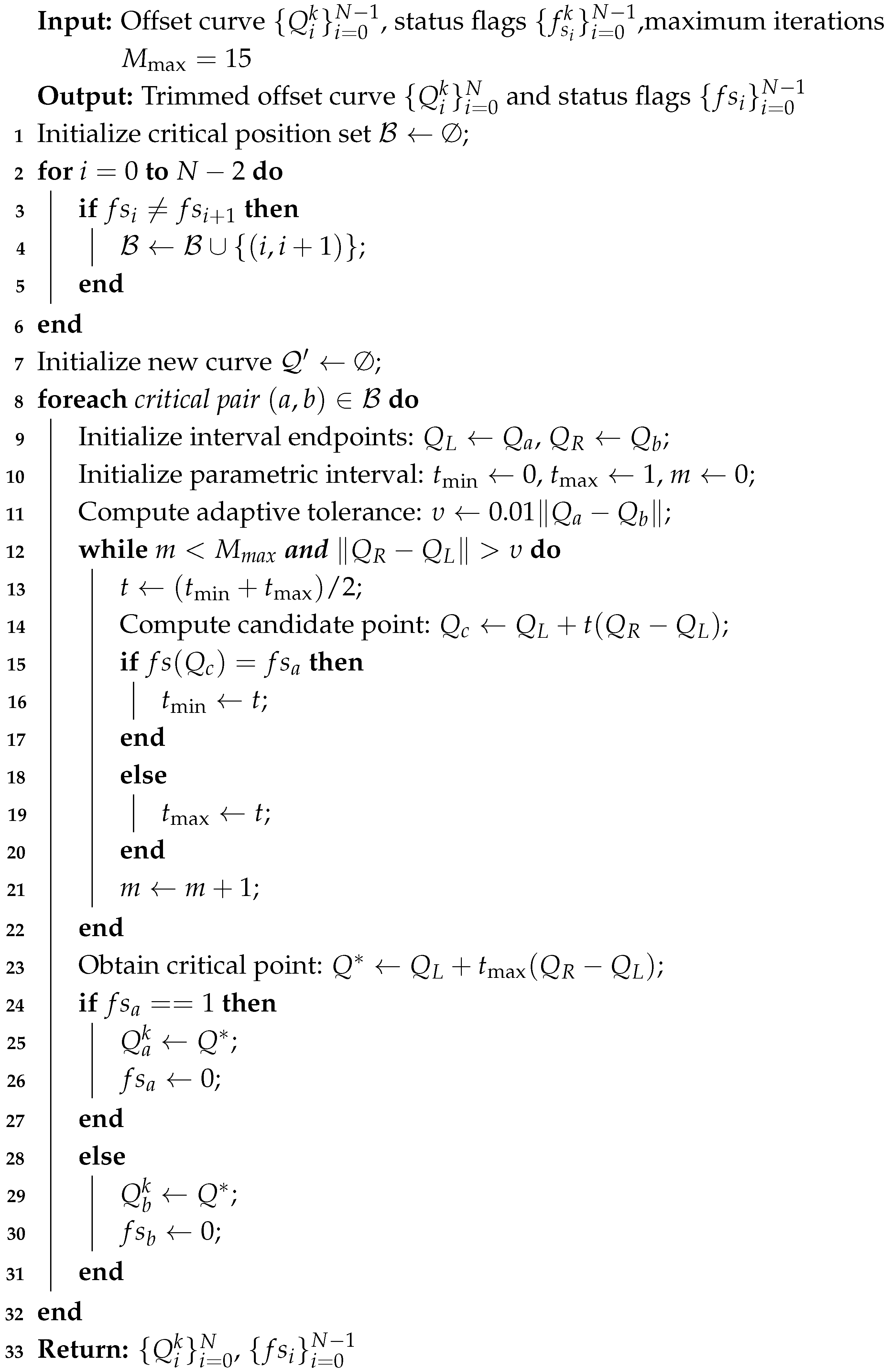
The self-intersecting point is then reclassified as non-intersecting, and its position is updated to the critical point calculated through bisection. This completes the critical trimming between intersecting and non-intersecting segments, with the detailed procedure outlined in Algorithm 6:
Through this algorithm, self-intersection points are located and trimmed at critical positions to facilitate subsequent smooth connections.
3.4.3. Path Generation
Following self-intersection trimming, points identified as self-intersecting are removed from each offset curve. The remaining segments are then evaluated for connectivity within a given threshold: starting with the first segment as the current segment, the starting point of each unconnected subsequent segment is checked. If the distance between this starting point and the endpoint of the current segment is below the specified threshold, the segment is connected to the current segment and merged into a continuous curve. The process continues by setting the next segment as the current segment for further detection. The detailed procedure is outlined in Algorithm 7.
The connected set is used as CC points, which are then converted into cutter location (CL) points to generate the final tool paths. For ball-end mills, this conversion is performed by offsetting each CC point along the surface normal direction by the tool radius
R:
where
is the unit normal vector at the corresponding CC point.
| Algorithm 6: Self-Intersection Removal with Critical Trimming |
 |
The trimming procedure in Algorithm 6 is essential for achieving a smooth CL trajectory. By removing self-intersections from the offset curve, the algorithm eliminates invalid loops and sharp corners that would otherwise introduce abrupt positional jumps in the CC points. The binary search precisely locates the critical boundary between the “clean” and “uncut” regions, and the curve endpoint is repositioned to this boundary. This ensures that the trimmed CC curve is continuous and free of spurious segments, which directly propagates to a smooth CL path through the normal offset in Equation (
19).
The complete workflow of self-intersection removal, trimming, and connection is illustrated in
Figure 9. Through this processing pipeline, the output tool paths are ensured to be free of self-intersections and maintain smooth continuity.
| Algorithm 7: Connection of Trimmed Curves |
 |
4. Experiments
In this section, the proposed method was applied to three models to compute corner cleaning regions and generate corresponding tool paths. Comparative studies were conducted against PM24, with results confirming the method’s effectiveness and computational efficiency. The implementation is carried out in C++ and runs on a workstation equipped with an Intel Core i5 3.60 GHz processor and 16 GB RAM. The experimental configuration maintained consistent machining parameters: preceding finishing operations employed a 6.0 mm ball-end tool under a 0.1 mm scallop height constraint throughout all tests.
For experimental consistency, the previous machining tool paths are set to achieve complete coverage of all accessible non-interference areas on the workpiece surface. This configuration closely mirrors practical corner cleaning applications, targeting the removal of residual material from geometrically inaccessible areas left by previous finishing operations.
4.1. Case Study 1
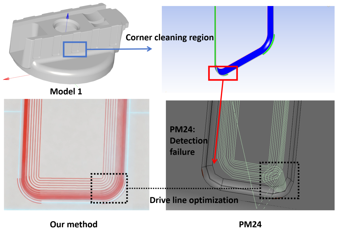
In case 1, a comparative study was conducted on workpiece model 1 using both the proposed method and PM24. The tool radius was determined to be 2.0 mm, selected according to the minimum absolute principal curvature of the surface to prevent over-cutting. The comparative results are summarized in
Figure 10.
The experimental results reveal a notable discrepancy in detection capability: although the workpiece surface exhibits geometric symmetry that produces symmetrically distributed corner cleaning regions, PM24 failed to identify one complete set of these areas. In contrast, the proposed method successfully detected all target regions with complete coverage paths. Moreover, within the area highlighted by the black line frame, the proposed approach generated drive curves demonstrating superior sweeping efficiency, confirming the effectiveness of the enhanced PCA methodology. The proposed method also exhibited superior performance in handling self-intersections, producing substantially smoother tool paths with seamless transitions at critical regions. This outcome validates the advanced capability of the self-intersection removal and trimming algorithms in maintaining path quality.
4.2. Case Study 2
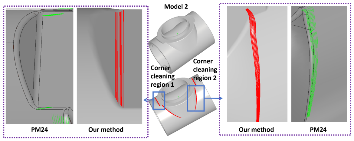
In case 2, a comparative analysis was conducted on workpiece model 2 using both the proposed method and PM24. Based on the minimum absolute value of the surface’s principal curvature, the tool radius was determined to be 1.0 mm. The experimental results are presented in
Figure 11.
Case study 2 demonstrates consistent detection capability between the proposed method and PM24, as both approaches successfully identified the same four corner cleaning regions indicated by red areas in
Figure 11. A detailed analysis is provided, focusing on two representative regions to highlight critical performance differences. In corner cleaning region 1, PM24 encountered tool path generation failures, while the proposed method consistently produced valid offset paths conforming to the chord error constraint. For corner cleaning region 2, the proposed method achieved complete and smooth path coverage, whereas PM24 generated discontinuous trajectories containing evident offset miscalculations. These comparative outcomes underscore the technical advantages of the proposed drive curve generation framework and its enhanced robustness in handling complex CAD structures.
4.3. Case Study 3
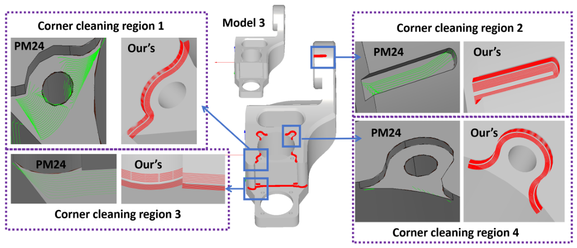
In case 3, a comparative analysis was conducted on workpiece model 3 using both the proposed method and PM24. Based on the minimum absolute value of the surface’s principal curvature, the tool radius was determined to be 2.0 mm. The experimental results are presented in
Figure 12, where tool paths generated by the proposed method and PM24 are marked in red and green, respectively, for each corner cleaning region.
Both methodologies successfully identified the same corner cleaning regions on this model, as marked by the four red zones in
Figure 12. Leveraging the model’s symmetrical configuration, four representative regions are analyzed to highlight critical performance distinctions. In regions 1 and 4, PM24 failed to produce valid tool paths, potentially due to directional computation errors arising from the surface’s closed parametric domains. Conversely, the proposed approach consistently generated valid offset paths conforming to the chord error constraint through a robust drive curve offset method, demonstrating enhanced compatibility with complex CAD representations.
For corner cleaning region 2, the proposed method generated smooth tool paths free of self-intersections through robust detection and trimming mechanisms, whereas PM24 produced paths with visible twisting and self-intersection defects that would compromise both machining efficiency and surface quality. This comparative outcome confirms the effectiveness of the proposed self-intersection removal and trimming strategy.
In corner cleaning region 3, the proposed method achieved superior path uniformity with complete path coverage of the target area. In contrast, PM24 produced paths exhibiting convergence-induced self-intersection at the leftmost section and insufficient path coverage restricted to the lower surface region. This inadequate path distribution would likely cause localized tool overloading during actual machining, potentially accelerating tool wear and compromising surface quality.
4.4. Machining Example
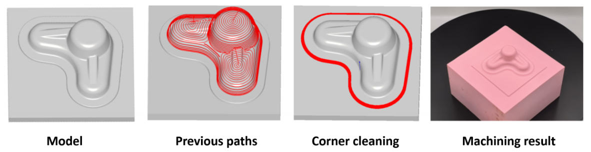
A real machining case is presented to validate the effectiveness of the proposed method. The experiment was conducted on a three-axis vertical machining center using an aluminum alloy 6061-T6 workpiece. As shown in
Figure 13, during the finishing stage of the input model surface, tool paths were first generated using a larger ball-end tool (radius
mm). However, a height difference exists between the lower surface of the model and the base platform, creating a peripheral right-angled corner region that prevents complete material removal with the current tool. By applying the proposed method, the corner cleaning regions were successfully detected, the appropriate tool radius was determined to be
mm according to the criterion in
Section 3.2, and corresponding cleaning paths were generated with a spindle speed of 12,000 rpm and feed rate of 600 mm/min. The resulting tool paths, shown as blue trajectories in
Figure 13, were executed to remove the residual material. Surface inspection after machining gave roughness values
and
, well within the finishing tolerance of
, and dimensional deviations measured at three locations were below
mm, confirming that the machined surface meets precision requirements. This machining case demonstrates the practical effectiveness of the proposed approach in real manufacturing scenarios.
4.5. Conclusion of the Experiments
To provide a rigorous quantitative assessment of the proposed method, we conducted a comparative performance analysis against PowerMill 2024 (PM24) using the three case studies described above. The following metrics were recorded for each test case: (1) total length of generated tool paths (in meters), (2) maximum scallop height error (in mm) and average scallop height error (in mm) over the machined surface, and (3) algorithm computation time (in seconds). The scallop height errors were evaluated by sampling the machined surface at a uniform grid resolution of 0.05 mm and computing the deviation from the designed surface. The results are summarized in
Table 1.
From
Table 1, the proposed method consistently produces shorter total path lengths than PM24, indicating higher sweeping efficiency. The maximum and average scallop height errors achieved by our method are also lower than those of PM24 across all three cases, confirming better surface quality. Although the computation time of our algorithm is slightly higher in each case (due to the additional optimization steps in enhanced PCA and self-intersection trimming), the increase is marginal (approximately 20–30%) and remains acceptable for practical offline CAM planning. These quantitative metrics substantiate our claims of superior sweeping efficiency, path quality, and computational robustness.
The comparative experiments validate the superiority of the proposed method, yielding three key conclusions:
Experimental results confirm that the proposed corner region detection method based on scallop analysis achieves higher accuracy. The drive curve construction algorithm and offset curve smoothing mechanism significantly enhance machining reliability for complex surfaces while maintaining path continuity.




 ,
,