1. Introduction
Robots have been widely deployed across industrial production scenarios in recent years. They drastically elevate manufacturing efficiency, reduce operators’ labor intensity, and provide critical technical support for advancing industrial automation. Nevertheless, practical robotic applications still face several prominent bottlenecks. First, motion precision deteriorates noticeably at both high and low joint velocities, restricting robot deployment in high-accuracy working tasks. Second, traditional industrial setups adopt physical isolation between humans and robots. Although this mode maximizes operator safety, it inflates equipment investment costs and hinders further productivity improvements. Third, human–robot collaboration (HRC) lacks direct physical interaction capability, which severely compromises collaboration flexibility. Real-time external force/torque sensing devices are therefore mandatory to realize safe physical human–robot contact during operation.
Under the conventional human–robot separation paradigm, collaborative manipulation relies on real-time joint torque perception to guarantee safe interaction. However, in unstructured environments, continuous dynamic robot motions and manipulator posture reconfiguration constantly alter the reference joint torque values, introducing severe interference to force-sensing precision. The literature [
1] demonstrates that terrain-adaptive foot placement and pose optimization redistribute the full robot load; without precise calibration of dynamic friction and inertial parameters, time-varying baseline drift will contaminate raw force measurement signals. Accordingly, high-fidelity dynamic parameter identification serves as the core basis for eliminating torque deviations induced by motion planning and enabling reliable force perception in human–robot interaction.
Resolving the above challenges hinges on accurate robot dynamic models, which play an irreplaceable role in advanced control algorithm design [
2], collision detection [
3], physical human–robot interaction [
4,
5], and multi-robot cooperative control [
6]. A precise dynamic model is also an indispensable prerequisite for boosting manipulator control performance and guaranteeing motion accuracy. Unfortunately, robot manufacturers rarely supply complete, high-fidelity dynamic models to end users. Meanwhile, dynamic parameters extracted via computer-aided design (CAD) software exhibit substantial deviations from those of physically deployed robots. Consequently, experimental identification has become the most reliable pathway to acquire accurate robot dynamic parameters [
7].
Existing experimental dynamic identification approaches fall into two primary categories: model-free and model-based identification. Model-free dynamic identification eliminates the requirement for predefined precise manipulator mathematical models. Using measured joint position and motor current signals, the entire robotic system is treated as an unknown nonlinear multi-input, multi-output (MIMO) system for identification. Representative model-free techniques include multilayer perceptron compensators [
8], Gaussian process regression [
9,
10], radial basis function network compensators [
11], and adaptive neural optimization frameworks [
12,
13]. Such methods feature strong flexibility, avoid cumbersome mathematical derivation, and can be readily adapted to diverse robot platforms. However, compared with model-based identification, model-free approaches consume excessive computational resources while delivering lower identification precision. Furthermore, the identified black box system cannot fully reflect all physical effects during robot operation [
14], and reliable estimation of inertial parameters cannot be guaranteed. These drawbacks render model-free methods unsuitable for high-precision parameter-dependent tasks, such as state observer design.
Model-based dynamic identification generally consists of four core steps: dynamic modeling, excitation trajectory optimization, parameter regression, and model validation. For dynamic modeling, the Newton–Euler formulation stands as the classic and most widely adopted method to derive manipulator dynamic equations. Specialized symbolic modeling toolboxes, including SYMORO [
15] and OpenSYMORO [
16], can rapidly linearize dynamic equations and greatly streamline modeling workflows. Gautier and Khalil [
17] proposed an efficient modeling strategy that extracts dominant variables and their internal correlations within dynamic models while minimizing the number of parameters required to characterize system behavior, laying a fundamental groundwork for subsequent parameter identification.
Base parameter sets have been extensively adopted in model-based dynamic identification, as they significantly enhance identification efficiency and accuracy while simplifying the overall identification pipeline. Even so, this technique carries obvious limitations: the linear joint friction model conventionally adopted fails to capture the nonlinear friction behavior present in real-world operation, leading to degraded identification precision. To mitigate this issue, Han et al. [
4] adopted the nonlinear Coulomb–viscous friction model [
18], while Dong et al. [
19] employed the Tustin friction model. Both models deliver more realistic representations of friction dynamics and improve parameter identification performance. Additionally, the Stribeck friction model [
20,
21,
22] is widely utilized to characterize low-speed joint friction in manipulators. By incorporating these nonlinear friction formulations, researchers can accurately describe manipulator dynamic properties and lay a solid foundation for high-precision parameter identification.
From an experimental implementation perspective, excitation trajectory design constitutes a critical prerequisite for accurate robot dynamic identification, and trajectory rationality directly determines the reliability of identification outcomes. To fully excite the system regression matrix and maximize parameter estimation accuracy, excitation trajectories must undergo rigorous optimization. Fifth-order polynomial excitation trajectories [
23] represent a prevalent effective solution, featuring few tunable parameters, simple computation, and zero velocity/acceleration boundary conditions at trajectory start and end points. These properties satisfy the smooth motion requirements of manipulators and align well with practical identification experiments. To suppress data acquisition noise and improve identification robustness, periodic Fourier series trajectories [
24,
25] have been proposed and applied; such trajectories possess stable frequency bands and demonstrate distinct advantages in data collection and post-processing. Over the past decade, fifth-order periodic Fourier series excitation trajectories have garnered growing research attention, as they integrate the merits of fifth-order polynomial profiles and periodic Fourier trajectories with superior smoothness and data processing compatibility. Common optimization metrics for excitation trajectories include the condition number of the full regression matrix [
26], sub-regression matrix condition numbers [
27], and the logarithmic determinant of the regression matrix [
28]. In summary, optimized excitation trajectory design represents a fundamental and effective method to improve experimental dynamic identification accuracy.
Accurate dynamic parameter estimation constitutes the core stage of manipulator dynamic identification. Conventional parameter estimation algorithms include least squares [
17], maximum likelihood estimation [
25], and Kalman filtering [
29]. While these methods enable rapid parameter solving, they suffer from notable deficiencies: (1) estimation results are highly susceptible to measurement noise and outliers; (2) the identified minimal parameter set often violates physical feasibility constraints; (3) enforcing physical constraints may degrade identification accuracy and push estimated parameters to the boundaries of physically feasible regions; (4) robot motion speed, system bandwidth, and mechanical structural limitations prevent full excitation of the regression matrix; and (5) most identification algorithms are built upon linear friction models, exhibiting poor compatibility with nonlinear friction formulations.
Current research schemes still possess evident drawbacks. The majority of existing methods only resolve isolated subproblems or achieve partial identification objectives, lacking comprehensive solutions to all core technical challenges. Few studies jointly integrate nonlinear friction models, iterative optimization strategies, and geometric calibration methods to solve manipulator base dynamic parameters. Most reported dynamic identification approaches fully linearize the entire dynamic model, which the existing literature verifies cannot accommodate nonlinear friction descriptions and fails to balance accurate friction nonlinearity characterization and identification precision.
The OLS-FBPE (Ordinary Least Squares Feasible Base Parameter Estimation) framework proposed by Sousa & Cortesão enforces linear matrix inequality (LMI)-based physical constraints on single-step least squares regression to filter unphysical inertial parameters. Nevertheless, the original OLS-FBPE architecture suffers from two critical flaws: (1) linear friction coefficients and inertial parameters are coupled within a single regression matrix, making it impossible to decouple strong nonlinear friction residuals from inertial identification bias, and (2) only linear Coulomb–viscous friction models are supported, with no compatibility for low-speed Stribeck nonlinear friction effects. To overcome these bottlenecks, this paper proposes a dual-layer hierarchical iterative optimization architecture that decouples offline nonlinear friction pre-identification and constrained inertial parameter regression with closed-loop residual feedback iteration, constructing a nested optimization loop absent from single-shot OLS-FBPE and weighted FBPE variants.
The remainder of this paper is organized as follows.
Section 2 elaborates on robot dynamic modeling and related fundamental theoretical background.
Section 3 details the proposed hierarchical iterative dynamic parameter identification algorithm.
Section 4 validates the effectiveness of the proposed method via physical experiments.
Section 5 summarizes the core contributions of this work and outlines future research directions, followed by concluding remarks.
2. Robot Dynamic Modeling and Fundamental Theories
The Newton–Euler recursive formulation is universally adopted to establish the dynamic model of an
degrees of freedom serial robot, expressed as:
where
denotes joint position,
denotes joint driving torque,
denotes joint friction torque,
denotes the symmetric positive definite mass matrix,
represents the centrifugal and Coriolis force vector, and
stands for the gravitational torque vector.
The linear Coulomb–viscous friction model is widely adopted for joint friction characterization in traditional robot dynamic modeling [
30]. This model features a simple linear structure where friction torque varies proportionally with joint velocity, and it introduces no extra unknown terms during regression matrix construction for identification. However, it cannot capture the intrinsic nonlinear characteristics of joint friction, and model uncertainty inevitably induces identification errors. The mathematical expression of the classical Coulomb–viscous friction model reads:
where
denotes the viscous friction coefficient,
represents the Coulomb friction coefficient, and
stands for the joint friction offset coefficient.
Equation (1) is linearized and converted into the product of a regression matrix and a standard dynamic parameter set, which is expressed as follows:
where
refers to the regression matrix,
is the number of joints,
represents the quantity of parameters in the standard parameter set, and
denotes the standard dynamic parameters of the whole robot. According to the linear Coulomb–viscous friction model (2), each link has 14 standard dynamic parameters, consisting of 11 inertial parameters and three friction parameters.
represents the standard dynamic parameters of the
link. The standard dynamic parameter set of each link
is given as follows:
,
. Where
denotes six components of the inertia tensor,
stands for the first-order moment of the inertia of link
,
refers to the mass of link
, and
represents the rotational inertia of joint axis
.
To reduce the dimensionality of parameters to be solved, the full standard parameter set can be simplified into a minimal base parameter set, and Equation (3) is re-linearized as:
where
is the reduced regression matrix corresponding to base parameters,
refers to the number of independent base parameters, and
denotes the vector of actual base inertial parameters. The mapping relation between standard and base parameters satisfies
, where
is a constant permutation matrix.
The dynamic characteristics derived from standard and base parameter sets are theoretically equivalent. Given m groups of sampled motion data, Equation (4) can be rewritten in batch matrix form:
where
,
, and
are the observation vector, observation matrix, and error vector, respectively, and they are defined as follows:
The base parameter vector can be preliminarily estimated via the least squares method:
The closed-form analytical solution of least squares is:
The residual error vector after parameter fitting is calculated as:
To ensure the physical feasibility of the solved base parameters, Equation (8) is transformed into an optimization problem constrained by linear matrix inequalities, which is the OLS-FBPE algorithm:
is defined as:
where
,
, and
is the
identity matrix. Equation (12) can be equivalently transformed into a non-strict linear matrix inequality by subtracting an infinitesimal positive scalar from the diagonal elements. Thus, Equation (12) can be regarded as a semi-definite programming optimization problem, which can be solved using the YALMIP [
31] toolbox in MATLAB2023.
3. Robot Parameter Identification Method
3.1. Nonlinear Friction Identification
As shown in Equation (2), the classical linear Coulomb–viscous friction model cannot fully capture joint nonlinear friction behaviors and will introduce large identification bias. Multiple studies have verified that viscous friction has a power law nonlinear correlation with joint velocity. Ref. [
4] defines viscous friction as a power function of angular velocity, forming the nonlinear Coulomb–viscous friction model:
where
, and the sign function is defined as:
Nevertheless, the nonlinear Coulomb–viscous model still fails to describe startup and low-speed friction characteristics of joints, so the standard Stribeck friction model is adopted for a more accurate friction torque expression:
where
is an empirical parameter representing the Stribeck velocity, and
is the maximum static friction force.
According to the analysis in the literature [
21], exponential velocity terms can better describe nonlinear viscous friction. Meanwhile, replacing the discontinuous
function with the arctangent function eliminates model discontinuity at velocity reversal points. On this basis, an improved Stribeck friction model is proposed in this paper:
where
denotes the power exponent of nonlinear viscous friction, and
is the smoothing coefficient of the arctangent term.
To calculate the robot’s friction torque separately, we analyze the composition of the robot’s joint torque. From Equation (1), it can be observed that the inertial torque depends only on the robot’s acceleration, while the Coriolis and centrifugal torques depend on the robot’s joint velocity and satisfy
. The gravitational term is only affected by the robot’s joint angles. To eliminate the inertial, Coriolis, centrifugal, and gravitational torques, a trajectory satisfying the joint friction torque is constructed as follows:
where
is the full trajectory period;
is the angular position of joint
;
represents the constant velocity magnitude of the u-th velocity group for joint
; U is the total number of velocity groups set for friction testing; and
stands for the duration of velocity switching phases.
To ensure smooth switching of the robot joint velocity, the following constraints are designed:
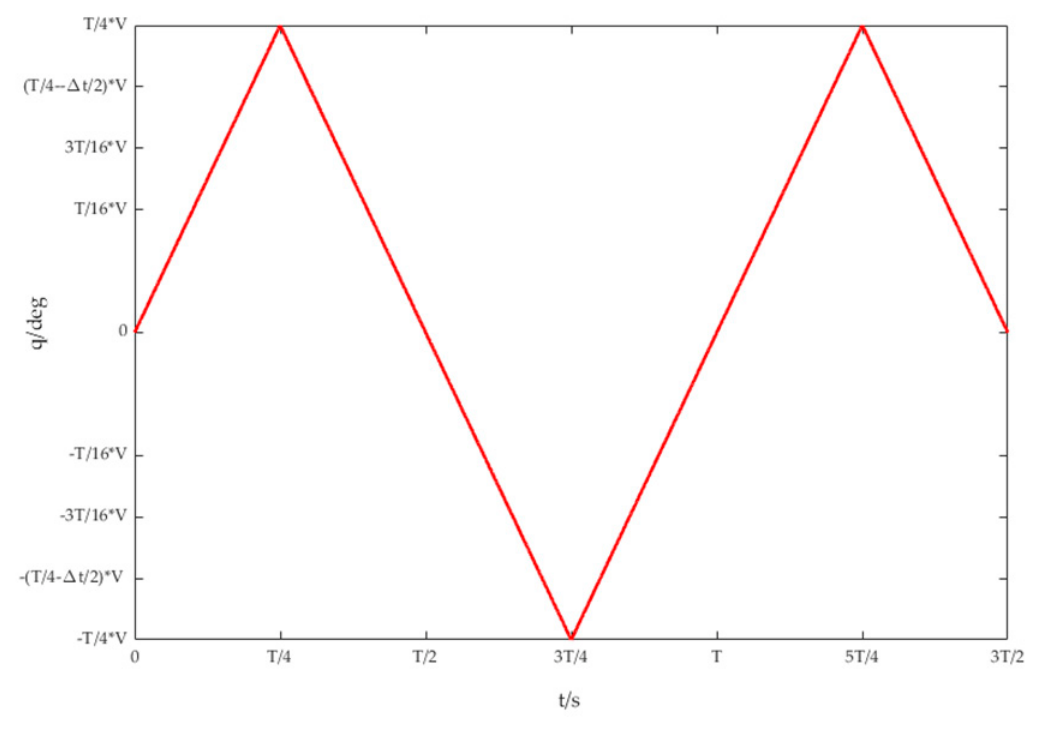
where
,
,
,
,
, and
are the coefficients of the velocity trajectory during the three commutation phases, as shown in the trajectory in
Figure 1.
The dynamic model (1) theoretically indicates that inertial torque is coupled with joint acceleration, gravitational torque is solely dependent on joint angles, and Coriolis torque is jointly determined by joint position and velocity. When joints move at strictly constant velocity, joint acceleration equals zero, eliminating all inertial torque contributions. The Coriolis term satisfies the symmetric identity
. Assuming that friction torque exhibits odd symmetry
, friction torque retains identical magnitude with reversed sign upon velocity reversal. If inertial, Coriolis, and gravitational torque components are fully eliminated or counterbalanced, pure friction torque can be isolated under constant velocity motion. For zero joint acceleration and reversed joint velocity, measured joint torque satisfies:
where the joint friction torque can be calculated as
.
Velocity continuity is enforced by setting joint angular velocity to zero at trajectory start and end points. The first half of each trajectory cycle is used to collect forward-direction friction torque data, while the latter half captures reverse-direction friction torque measurements. This trajectory framework is executed to sample joint torque signals across multiple discrete velocity levels for each joint. With m groups of velocity setpoints, the acquired discrete friction torque dataset is denoted as
. In this work, the interior-point optimization method is adopted to identify nonlinear friction parameters, with physical feasibility constraints embedded within the optimization objective:
3.2. Inertial Parameter Identification
Equation (5)
demonstrates that dynamic model identification can be formulated as a multi-output multivariate linear regression problem, where
acts as the response vector,
represents the design regression matrix,
corresponds to the regression coefficient vector, and
denotes the Gaussian noise error term with the following covariance property:
where
denotes the mathematical expectation operator, and
is an
diagonal matrix whose diagonal entries equal the noise variance of each joint’s driving torque measurement.
The stacked observation matrix and torque response vector are constructed from sampled motion data following Equation (5), and the base parameter vector
is solved via the standard least squares closed-form solution:
The variance of each estimated base parameter is extracted as the diagonal entries of the covariance matrix:
where
denotes the operator extracting diagonal elements from a matrix. Equation (18) presents the ordinary least squares solution minimizing the L2 norm of residuals; however, this estimator yields suboptimal parameter variance performance. Weighted least squares (WLS) is introduced to optimize parameter variance distribution, which requires prior estimation of the noise covariance matrix
.
First, compute the residual vector representing the deviation between model-predicted torque and measured torque:
where
has the dimension of
. It can be rearranged into matrix E with dimension
, whose rows store residuals of each joint.
The value of
can be estimated by E as follows:
where
is the
diagonal element of
,
represents the
row of matrix E, and
represents the L2 vector norm. Notably,
can be applied to the Kalman filter design of external force observers, and
serves as the weighting coefficient of WLS.
After estimating
, the weighted least squares solution for base parameters is derived as:
where M is an
block-diagonal matrix with m copies of
distributed along its main diagonal. The parameter variance under weighted least squares is expressed as:
To prevent solved dynamic parameters from converging to the boundaries of physically feasible regions, the optimization objective is augmented with a reference parameter solution term to guide parameter estimation toward physically realistic values. The complete constrained optimization formulation is defined as:
where
denotes the reference dynamic parameter, and
represents the Euclidean L2 distance metric.
A refined geometric inertial parameter distance metric proposed in [
32,
33] is further incorporated into the cost function to improve constraint robustness:
3.3. Robot Dynamic Parameter Identification
To achieve high-precision dynamic parameter estimation, a hierarchical iterative optimization framework is proposed, which decouples the robot dynamic model into two independent components: inertial torque terms and friction torque terms:
where
and
represent inertial torque and friction torque, respectively,
is the regression matrix excluding all friction-related terms, and
denotes the minimal inertial base parameter vector stripped of friction coefficients.
The full base parameter vector
can be partitioned into two disjoint subsets: inertial base parameters
and friction parameters
. Equation (5) is, therefore, rewritten in block form:
The pure inertial torque signal with friction components eliminated is isolated as:
Conversely, nonlinear friction torque can be recovered from measured torque and predicted inertial torque:
The hierarchical iteration loop adopts dual joint convergence criteria combining torque RMSE threshold and friction parameter deviation threshold, with a hard maximum iteration limit to avoid infinite loop:
- (1)
Torque residual RMSE threshold: per joint; total six-joint sum threshold .
- (2)
Friction parameter deviation threshold: , defined as the L2 norm difference of the full Stribeck friction parameter vector between two consecutive iterations.
- (3)
Hard maximum iteration count: iterations; iteration terminates automatically once reaching even if criteria unmet.
The detailed identification workflow is summarized as follows. The core principle of the hierarchical iterative algorithm integrates identification residuals generated in each iteration back into friction or inertial torque calculations, enabling progressive error correction through repeated alternating identification of friction and inertial parameters. The primary optimization objective is to minimize overall torque identification residuals, achieving tight fitting between model predictions and measured torque data and ensuring that the solved dynamic model faithfully reflects the physical motion characteristics of the physical robot. Convergence evaluation is performed using torque RMSE and friction parameter deviation metrics after each round of inertial and friction parameter regression. Iterative correction cycles continue until both convergence criteria are satisfied, yielding high-fidelity full dynamic parameter sets.
3.4. Friction Compensation
During robot dynamic parameter identification, the Stribeck friction model encapsulates coupled Coulomb, viscous, and static friction effects, featuring strong nonlinear attenuation, hysteresis, and time-varying behavior at low joint velocities. Reliable friction compensation must simultaneously satisfy two core requirements: capturing temporal motion features consistent with friction hysteresis and adhering to fundamental physical friction laws to avoid unphysical model outputs.
Conventional compensation strategies suffer from inherent drawbacks. Analytical Stribeck models rely on precisely calibrated physical friction parameters and lack adaptability to time-varying friction drift and complex nonlinear coupling under variable working conditions. Standard data-driven LSTM networks can capture temporal friction hysteresis but lack embedded physical constraints, frequently generating physically implausible friction torque predictions. Additionally, pure data-driven neural networks must relearn all core Stribeck nonlinear features from scratch, leading to slow training convergence and poor generalization performance, especially within low-speed regions dominated by pronounced Stribeck effects. Vanilla RNN and GRU architectures fail to model long-term temporal friction dependencies, as joint Stribeck friction states rely on historical velocity sequences spanning 5–8 control cycles, and standard RNNs suffer irreversible gradient vanishing during backpropagation over long time series.
To address the above limitations, this paper adopts a physics-informed LSTM (PI-LSTM) network for Stribeck friction compensation, which unifies physical prior modeling and data-driven temporal sequence fitting and delivers three key advantages. First, core physical features of the Stribeck friction model are embedded into the network input layer, guiding the model to prioritize critical friction characteristics, eliminate redundant feature learning, accelerate training convergence, and boost fitting accuracy within low-speed nonlinear operating regions. Second, hard physical constraint penalties are integrated into the composite loss function to enforce network outputs to comply with fundamental friction physical laws, eliminating the invalid unphysical predictions typical of purely data-driven neural networks. Third, lightweight optimization of input feature construction and loss function formulation balances temporal sequence fitting performance and real-time computational efficiency for practical engineering deployment. The proposed PI-LSTM retains the adaptive capacity of standard LSTM for time-varying friction while introducing physical interpretability, overcoming the inherent defects of both analytical friction models and unconstrained recurrent neural networks. The architecture achieves high-precision, robust Stribeck friction compensation and provides an advanced temporal modeling paradigm for robot dynamic parameter identification.
The ablation study in
Table 1 compares friction compensation RMSE across PI-RNN, PI-GRU, and PI-LSTM trained on identical datasets. PI-LSTM reduces overall torque RMSE by 19.7% relative to PI-RNN and 11.3% relative to PI-GRU, with a 27.2% error reduction specifically within low-speed Stribeck nonlinear regions compared with PI-RNN. The dedicated forget–input–output gate structure of LSTM enables selective retention of historical motion features critical for modeling friction hysteresis, a capability lightweight recurrent units (RNN/GRU) cannot replicate.
3.4.1. Temporal Characteristics of the Friction Model
Conventional LSTM networks only ingest angular velocity and acceleration sequences as raw inputs and must independently learn friction nonlinearity during training. In contrast, PI-LSTM embeds explicit Stribeck physical prior features directly into the input vector to guide model learning, with the full input feature vector defined as:
where t denotes the discrete current time step;
is the LSTM input sequence length aligned with robot control cycles to fully cover the temporal dependency window of friction hysteresis;
and
represent angular velocity and acceleration sequences over the preceding k time instants,
;
encodes friction direction physical prior information;
embeds the Stribeck nonlinear attenuation prior term; and
is the empirical characteristic Stribeck velocity guiding the network to focus on low-speed friction dynamics, and the total input feature dimension equals
.
PI-LSTM maintains the standard gating architecture of vanilla LSTM, with physical guidance solely implemented via customized input feature construction. The complete network update formulations are presented below:
where
is the forget gate weight,
is the forget gate bias,
is the hidden state of the previous moment,
is the number of hidden layer neurons, and
refers to the activation function.
where
denote weight matrices of the input gate or cell state,
represent corresponding bias terms, and
is the hyperbolic tangent function.
where
denotes the Hadamard product and
is the cell state of the previous moment.
where
and
are output gate weights.
where
is the preliminary predicted friction torque of PI-LSTM.
The composite loss function of PI-LSTM integrates weighted fitting loss and physical constraint penalty loss to eliminate unphysical torque outputs characteristic of unconstrained LSTM networks, formulated as:
where
is the physical constraint weight, balancing fitting accuracy and physical characteristics to avoid fitting deviation from excessive constraints or invalid weak constraints.
denotes basic temporal mean square error loss ensuring fitting precision.
stands for physical constraint loss composed of three core terms, complying strictly with Stribeck friction laws.
The baseline fitting loss
quantifies the squared deviation between PI-LSTM predicted friction torque and measured friction torque:
where
is the total number of time series samples and
is the measured Stribeck friction torque. It is obtained by subtracting inertia and damping terms from the measured joint driving torque:
where J is the moment of inertia and B is the viscous damping coefficient.
The physical constraint loss term
aggregates three independent penalty components: direction constraint loss, amplitude limit constraint loss, and Stribeck nonlinear characteristic constraint loss, formulated as:
where
stands for direction constraint loss,
is amplitude constraint loss, and
is Stribeck nonlinear constraint loss. The detailed mathematical definitions of each penalty term are:
For direction constraint loss , a positive penalty is imposed when to penalize friction torque predictions opposing physical friction direction; zero penalty is applied when the sign relation satisfies physical friction rules. For amplitude constraint loss , penalties equal the excess magnitude when predicted friction torque exceeds the maximum physical friction limit , with zero penalty for valid torque magnitudes. For Stribeck nonlinear constraint loss , is a small regularization constant to avoid division by zero, and is an empirical constant defining the maximum allowable friction torque per unit angular velocity. At low angular velocities, the ratio tends to exceed , activating the penalty term to force the network to output larger friction torque values at low speeds consistent with the Stribeck effect; the penalty vanishes only when the friction magnitude satisfies the required low-speed nonlinear growth property.
3.4.2. Convergence Analysis of Physics-Constrained Loss Function
The composite loss function consists of a strictly convex MSE fitting term and three convex penalty functions within . Given the bounded feasible domain of measured friction torque , the full loss function satisfies strong convexity with a uniform lower bound. Under Adam gradient descent training with bounded learning rates, the training loss sequence decreases monotonically and converges uniquely to the global optimal solution, eliminating local minimum traps prevalent in purely data-driven LSTM training.
3.4.3. Final Compensation Formula
After completing PI-LSTM offline training, the network is embedded into the robot real-time control loop. It receives real-time joint angular velocity, angular acceleration, and embedded Stribeck physical prior features as inputs and outputs that predict friction torque
. The final friction-compensated driving torque command for joint motor control is defined as:
where
denotes the raw torque command output from the motion controller, and
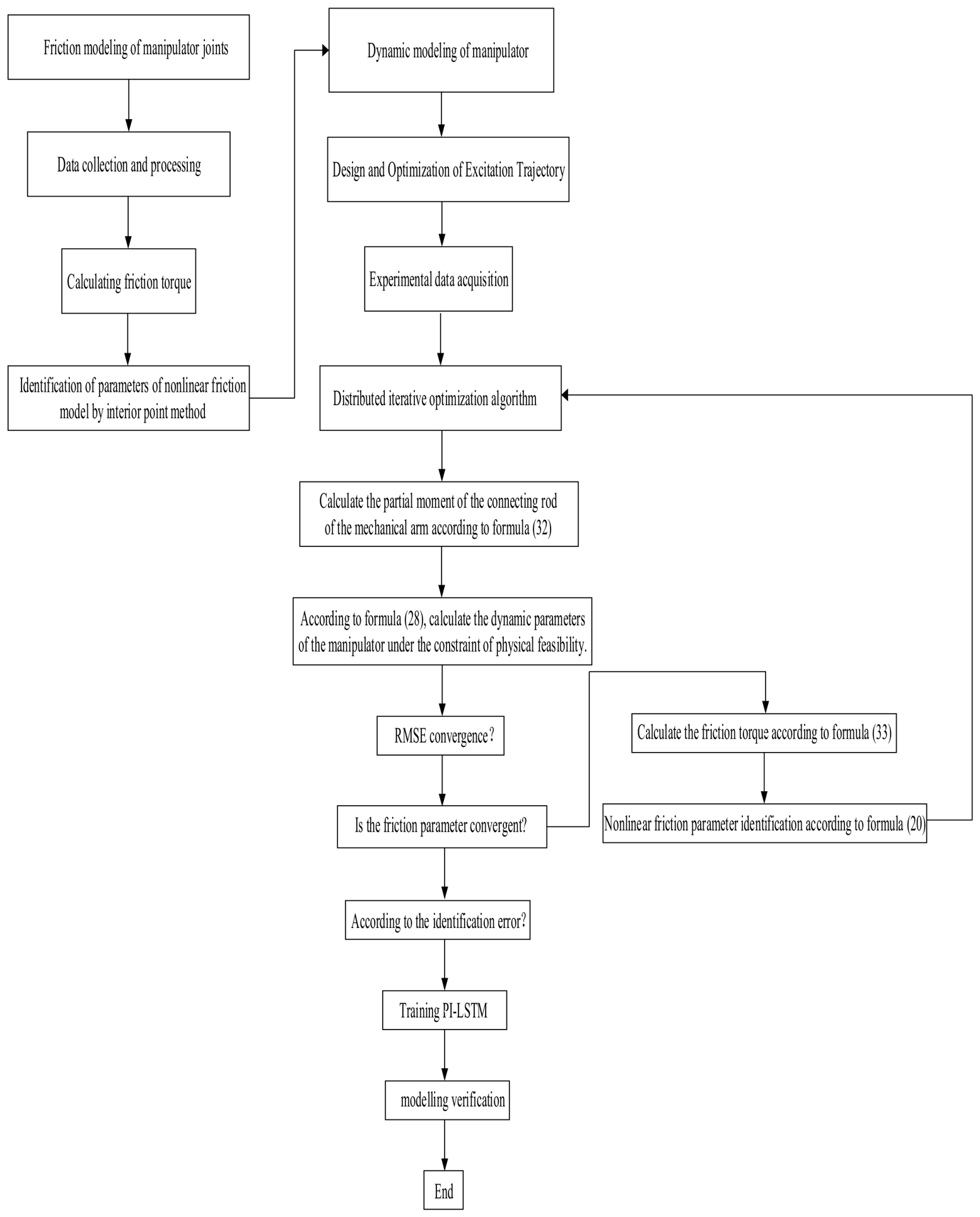
represents the friction-compensated driving torque directly issued to joint motors to realize high-precision Stribeck friction compensation. The complete robot dynamic parameter identification workflow is visualized in
Figure 2, and the full hierarchical iterative identification logic is formalized in Algorithm 1.
| Algorithm 1 Hierarchical Iterative Dynamic Parameter Identification |
.
.
1: // Layer 1: Offline Nonlinear Friction Pre-Identification.
2: Generate constant-velocity bidirectional friction trajectory per joint.
.
4: Solve improved Stribeck parameters via constrained interior-point optimization.
.
do.
7: // Layer 2: Constrained Inertial Parameter Regression.
.
signal.
(Proposed-FBPE).
.
.
.
14: // Closed-loop residual feedback to Layer 1.
.
.
17: end while.
18: Train PI-LSTM with converged friction residual dataset for dynamic friction compensation.
. |
4. Experimental Results and Analysis
4.1. Robot Kinematics Description
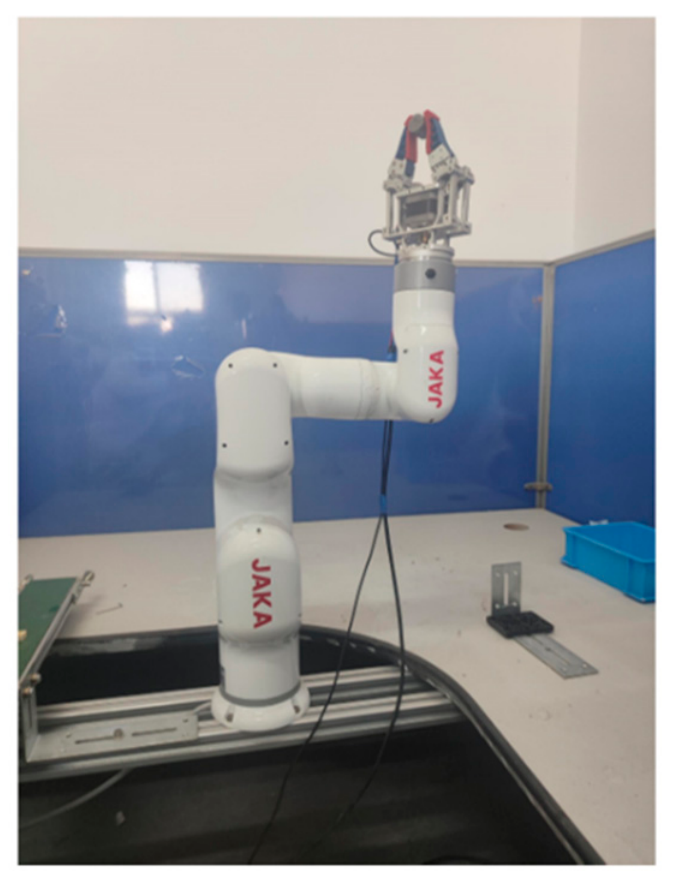
The identification test platform adopted in this work is a JAKA Mini Cobo six degrees of freedom serial collaborative manipulator, as shown in
Figure 3. This robot achieves a repeat positioning accuracy of
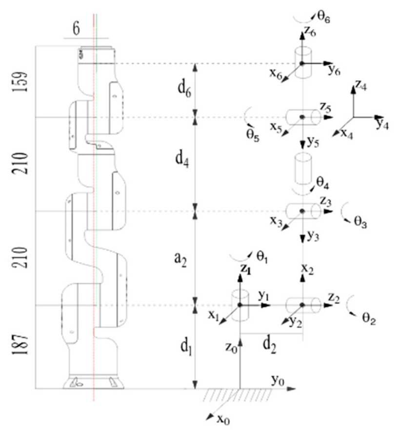
mm, a rated payload of 3 kg, and a maximum working radius of 580 mm, making it widely applicable to industrial assembly, welding, polishing, and other precision manufacturing tasks. Dynamic modeling of the manipulator relies on homogeneous coordinate transformation matrices for each rigid link, so kinematic modeling is completed using the modified Denavit–Hartenberg (MD-H) convention. The link coordinate frame layout of the manipulator is illustrated in
Figure 4, defined by four standard MD-H parameters: link twist angle
, joint rotation angle
, link offset
, and link length
. The complete MD-H parameter table is provided in
Table 2.
The experimental platform is the torque-sensorless JAKA Mini Cobo collaborative robot. Joint driving torque is indirectly calculated from measured motor phase current signals via the torque conversion formula:
where
,
, and
represent gear ratio, motor torque constant, and current vector, respectively.
Equation (46) only accounts for electromagnetic output torque of the drive motor and ignores nonlinear friction inside harmonic reducers, introducing systematic measurement bias at low joint velocities, as thoroughly validated in reference [
34]. For gear-driven robots without external joint torque sensors, reducer hysteresis and static friction offset contaminate raw torque estimation signals and directly degrade the accuracy of friction parameter identification. This paper implements a two-stage compensation scheme to eliminate reducer friction interference: first, static friction offset of each joint reducer is calibrated under zero-velocity stationary conditions, with the constant offset subtracted from raw torque estimates; second, reducer viscous friction terms correlated with angular velocity are integrated into the joint global friction model during the initial friction pre-identification stage, and their coefficients are solved synchronously alongside link Stribeck friction parameters.
4.2. Robot Excitation Trajectory Design
Excitation trajectory design encompasses two core tasks: selecting an appropriate trajectory formulation and optimizing trajectory coefficients to maximize regression matrix excitation. This work adopts fifth-order periodic Fourier series trajectories to elevate the signal-to-noise ratio of sampled measurement data. Repeated cyclic sampling and signal averaging mitigate random acquisition noise and simplify filter cutoff frequency selection in subsequent data preprocessing. The complete trajectory mathematical formulation is defined as:
where
denotes trajectory cycle times,
is the fundamental frequency,
is the harmonic order of the Fourier series, which is normally set to five, and
is the cycle count.
,
, and
are undetermined coefficients of the Fourier excitation trajectory.
To guarantee robot operational safety, joint angular position, velocity, and acceleration along excitation trajectories must be constrained within mechanical hardware limits. Additionally, joint velocity and acceleration must equal zero at trajectory start and end instants to satisfy smooth motion boundary conditions. Traditional trajectory optimization minimizes the regression matrix condition number; this paper adopts a more computationally efficient objective function referenced in the literature [
7] as the optimization cost metric:
Thus, the excitation trajectory can be expressed as:
where
,
,
,
,
, and
denote the minimum and maximum joint position, velocity, and acceleration, respectively.
and
stand for the start and end time.
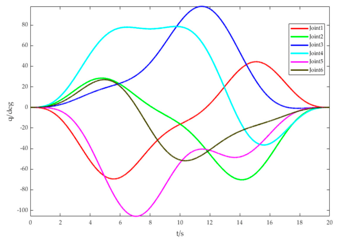
In experimental testing, the excitation trajectory optimization problem is solved via the C-implemented NLOPT nonlinear optimization library, and the final optimized excitation trajectory profile is visualized in
Figure 5.
4.3. Data Filtering
A combined filtering strategy integrating average filtering, Butterworth filtering, and zero-phase filtering, supplemented by smoothing processing, is adopted to complete data filtering. Firstly, average filtering is used to preprocess the original signal; secondly, the minimum order and normalized cutoff frequency of the filter are solved via the buttord function, and the Butterworth filter coefficients are calculated using the butter function; thirdly, zero-phase bidirectional filtering of the signal is realized by means of the filtfilt function, which effectively reduces phase delay and distortion of the signal; and finally, smoothing processing of the filtered data is completed by the smooth function with locally weighted scatterplot smoothing (LOWESS).
The squared magnitude frequency response of an N-order Butterworth low-pass filter is defined as:
where
is the square of the filter amplitude frequency response,
denotes cutoff angular frequency, and N represents filter order.
The mathematical formulations for forward and backward zero-phase filtering stages are:
Backward filter:
where
is the filtered output signal,
denotes filter coefficient,
is the input signal to be filtered, and
stands for filter order.
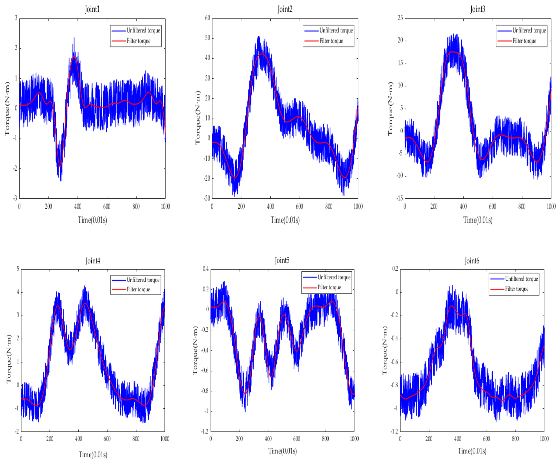
Based on frequency domain analysis of sampled robot motion signals, the system sampling frequency is configured to 50 Hz. The passband cutoff frequency is set to 1 Hz, the stopband cutoff frequency is 5 Hz, the maximum passband ripple is limited to 1 dB, and the minimum stopband attenuation is set to 15 dB. The filtering performance on joint torque signals is illustrated in
Figure 6. Comparative analysis confirms that the proposed composite filter effectively suppresses high-frequency measurement noise, yielding smooth torque waveforms free of random jitter while fully preserving the overall trend and key dynamic features of the original raw signal, verifying the validity and practical applicability of the multi-stage filtering pipeline.
4.4. Friction Parameter Identification
Prior to executing the full hierarchical iterative dynamic parameter identification algorithm, pre-identification of joint nonlinear friction parameters is mandatory. Following the single-joint friction torque acquisition methodology outlined in
Section 3.1, each joint of the six degrees of freedom manipulator is independently driven across a wide range of discrete constant velocities to collect comprehensive friction characteristic measurement data. Multiple repeated identification trials are conducted at each velocity setpoint to improve data robustness. The full set of joint velocity test points (unit: deg/s) includes: 0.0001, 0.0008, 0.01, 0.05, 0.1, 0.2, 0.3, 0.4, 0.5, 0.6, 0.7, 0.8, 0.9, 1, 1.1, 1.3, 1.5, 1.7, 1.8, 2.3, 2.6, 2.8, 3.3, 3.7, 4.1, 4.5, 5.5, 6, 8.7, 10, 13.3, 16, 21, 24, 32, 37, and 45.
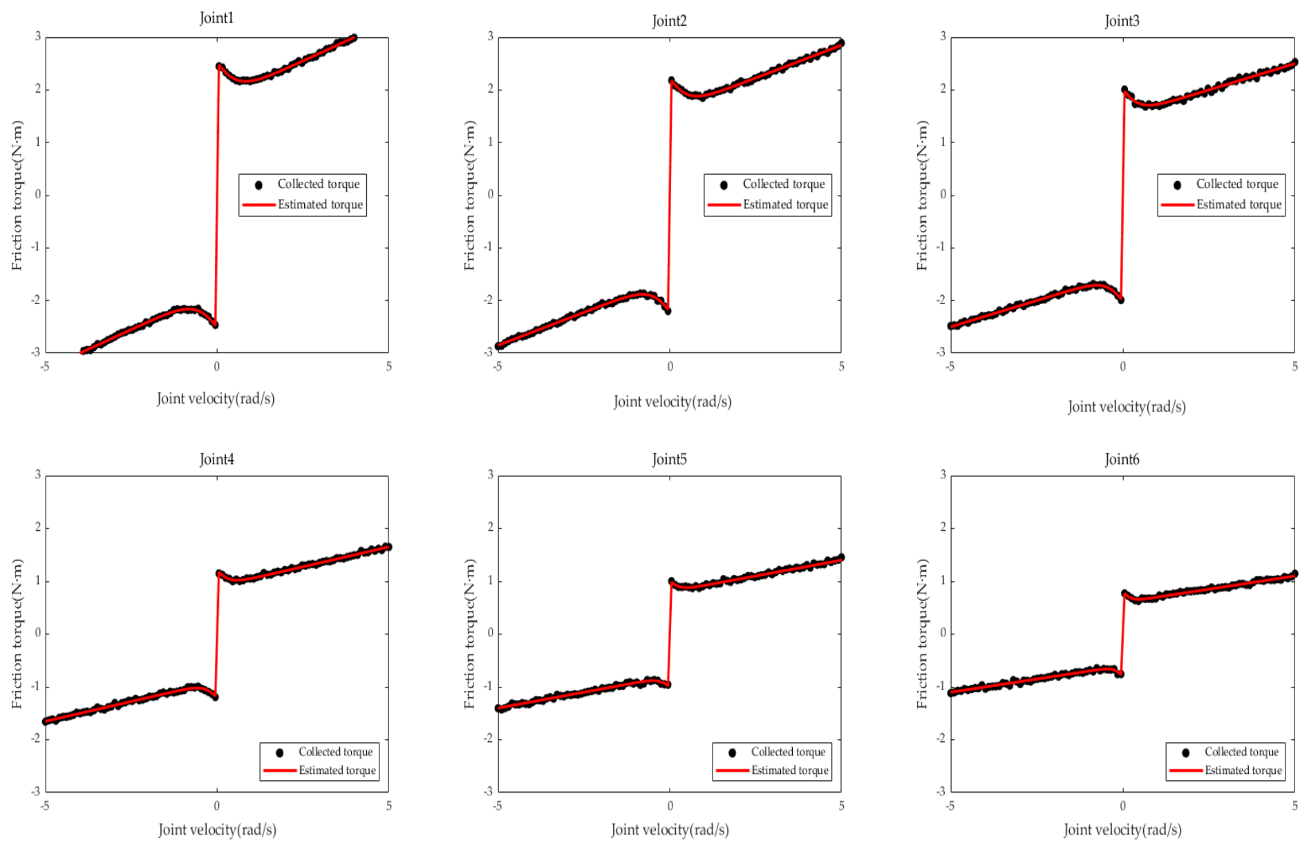
The friction pre-identification trajectory cycle duration is set to 12 s. Only data sampled during steady constant velocity motion phases are retained for friction parameter regression; acceleration and deceleration transient segments are discarded to eliminate interference from inertial and Coriolis torque components. Accurate friction torque calculation requires paired sampling points with identical joint angular position and equal-magnitude, opposite-direction joint velocity. Qualified paired measurement points are averaged to reduce random sampling errors. After data acquisition and preprocessing, the interior point convex optimization method is deployed to solve the full set of improved Stribeck friction parameters. The friction model fitting results are visualized in
Figure 7, and the complete solved friction coefficient values for all six joints are summarized in
Table 3.
To quantitatively validate that the proposed improved Stribeck friction model outperforms the nonlinear Coulomb–viscous model and standard discontinuous Stribeck model, total six-joint friction fitting RMSE values for all candidate models are computed and listed in
Table 4. The cumulative RMSE of the linear Coulomb–viscous friction model equals 3.149, the standard discontinuous Stribeck model yields a total RMSE of 3.284, the arctangent-smoothed standard Stribeck model achieves 2.552, and the fully improved Stribeck model proposed in this paper attains a minimum cumulative RMSE of 2.179. The proposed improved Stribeck friction model delivers superior fitting performance and aligns most closely with the actual nonlinear friction behavior of manipulator joints. Based on these verified friction parameter results, the hierarchical iterative dynamic parameter identification workflow is executed to solve full inertial base parameters.
4.5. Parameter Identification Results
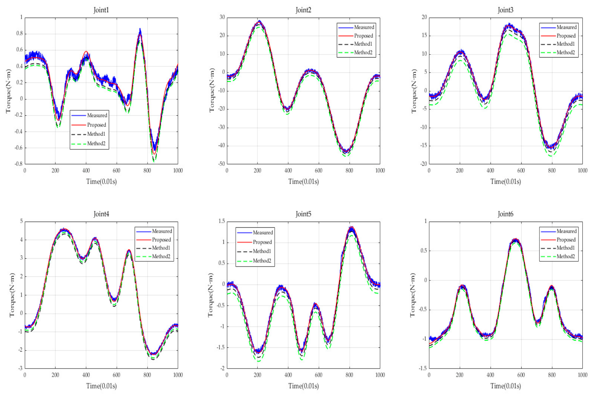
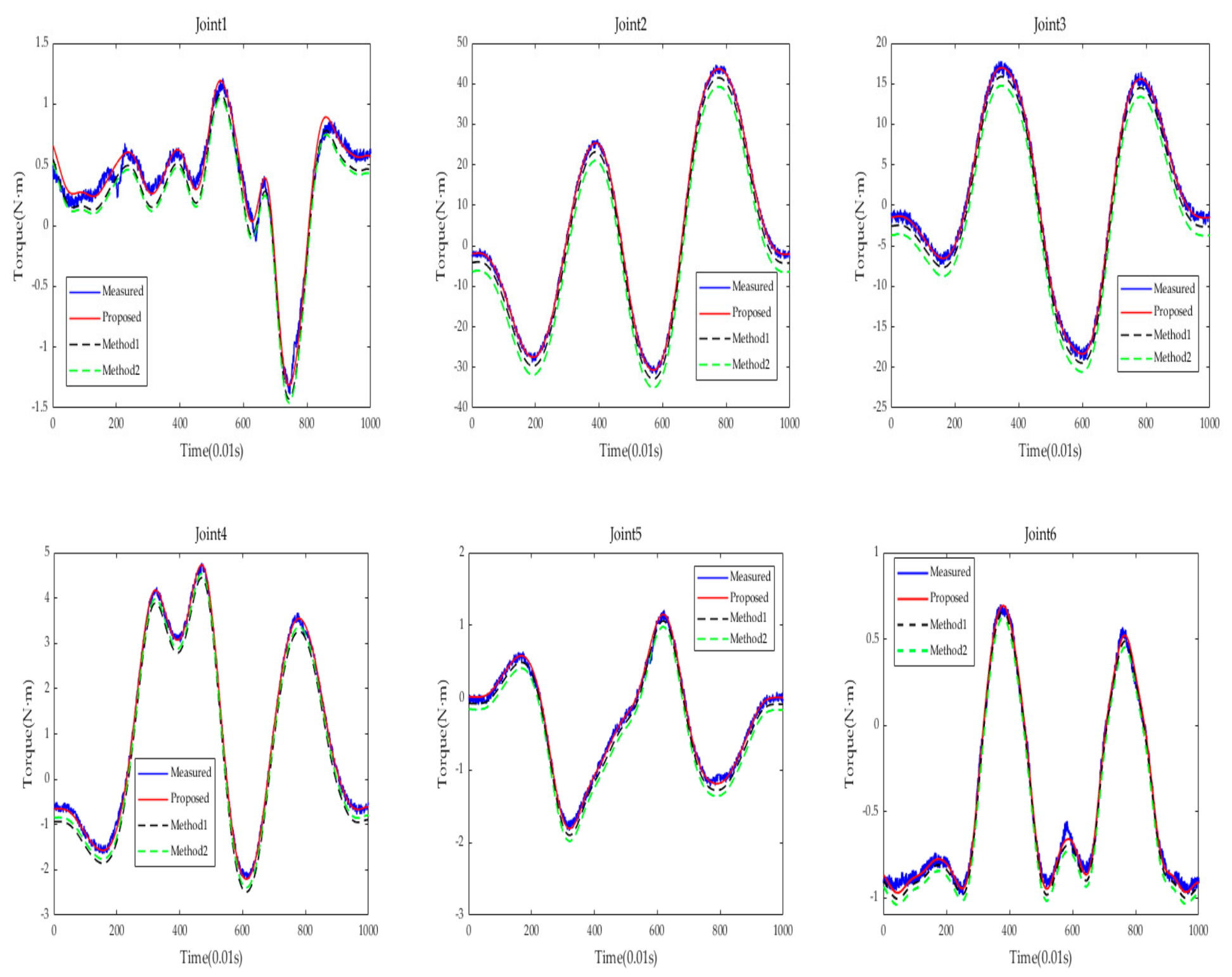
Figure 8 visually compares torque fitting curves generated by competing identification algorithms. Blue solid curves represent measured raw joint torque data; red curves denote torque predictions from the proposed hierarchical iterative constrained algorithm (Proposed-FBPE). Compared with Method 1 (WLS-FBPE, black curves) and Method 2 (LS-FBPE, green curves), the Proposed-FBPE torque predictions exhibit the tightest alignment with measured torque waveforms and superior overall fitting performance. Under high-torque operating conditions, Method 1 and Method 2 display obvious trajectory deviation and pronounced accuracy degradation, while the proposed algorithm maintains consistent fitting precision across the full torque operating range.
To quantitatively evaluate the identification performance of the hierarchical iterative optimization algorithm proposed in this paper, we deploy the aforementioned nonlinear friction identification scheme together with the two-layer iterative optimization framework to calibrate the complete dynamic parameters of the manipulator. Following the layered identification logic, we first extract friction components from joint torque measurements for nonlinear friction parameter estimation and then conduct constrained regression on inertial parameters with iterative residual correction. After the iteration process meets the preset convergence thresholds, we obtain a full set of calibrated dynamic parameters. All detailed numerical results of the identified inertial and friction coefficients are collated and presented in the table below for subsequent quantitative comparison with benchmark algorithms. The specific identification results are shown in
Table 5.
Six mainstream identification strategies are selected for side-by-side comparative evaluation, namely, LS, WLS, unconstrained Proposed, LS-FBPE, WLS-FBPE, and the proposed Proposed-FBPE algorithm. Among them, LS-FBPE, WLS-FBPE, and Proposed-FBPE incorporate linear matrix inequality physical feasibility (PFC) constraints during regression, while LS, WLS, and the unconstrained Proposed algorithm perform parameter estimation without physical bound restrictions. All six methods utilize identical preprocessed experimental excitation trajectory datasets to guarantee fair comparison, and working condition VT1 is adopted as the benchmark scenario to quantify algorithm performance and validate the superiority of the proposed framework.
Table 6 records the per-joint torque fitting RMSE and cumulative total RMSE of each algorithm. Lower RMSE values indicate smaller discrepancies between model-predicted torque and actual measured torque, which means the identified dynamic model better matches the real physical characteristics of the manipulator. Under working condition VT1, the total RMSE of the unconstrained Proposed algorithm reaches 27.329, whereas the total RMSE values of the standard least squares and weighted least squares methods are 39.542 and 35.505, respectively. This evident gap demonstrates that the hierarchical iterative optimization architecture can effectively suppress systematic modeling errors and deliver much higher identification precision. The dual-layer nested iteration design continuously eliminates the offset between theoretical torque outputs and practical robot dynamic responses, enabling the calibrated model to accurately reflect real motion characteristics under diverse operating states.
Identification algorithms satisfying PFC constraints yield remarkably improved results compared with unconstrained ones. Under the VT1 condition, the total RMSE of LS-FBPE drops by 6.516 against LS, WLS-FBPE decreases by 6.029 versus WLS, and Proposed-FBPE falls by 2.431 relative to Proposed. PFC constraints standardize parameter estimation, making identified parameters conform better to actual robotic dynamic properties and boosting identification accuracy and reliability.
To further verify the universal compatibility of the Proposed-FBPE algorithm with various friction models and quantitatively prove the advantages of nonlinear friction modeling over linear counterparts, a series of comparative experiments are carried out. For the sake of experimental fairness, the identical Proposed-FBPE identification framework is adopted for all four friction models. Traditional LS and WLS methods show prominent defects when combined with nonlinear friction expressions, as they cannot decouple nonlinear friction residuals from inertial parameter bias. The four friction models adopted in the contrast tests are the linear Coulomb–viscous model (Equation (2)), the nonlinear Coulomb–viscous model (Equation (13)), the standard Stribeck model (Equation (14)), and the improved Stribeck model proposed in this paper (Equation (15)).
The cumulative six-joint RMSE results under trajectory VT1 are listed in
Table 7. The comparison results clearly reveal that all nonlinear friction models achieve lower total torque error than the linear Coulomb–viscous model under the same identification framework. Throughout the whole iterative calibration process, the hierarchical iterative correction logic remains consistent for all four friction models. The superior capacity of nonlinear friction models to describe low-speed Stribeck hysteresis and velocity-dependent viscous nonlinearity greatly reduces identification residuals, which is the core source of accuracy elevation.
4.6. Model Verification
To further validate the generalization ability and practical reliability of the dynamic model calibrated via the Proposed-FBPE algorithm, an independent set of verification trajectories separate from the excitation trajectories is designed, as shown in
Figure 9. The data acquisition sampling frequency remains consistent with that used during parameter identification. The dynamic model solved from excitation trajectory data is employed to predict joint torque under the new verification motion profile, and predicted torque curves from different algorithms are contrasted against measured torque signals. The torque curve of the proposed Proposed-FBPE method exhibits far better coincidence with measured values than the curves of WLS-FBPE and LS-FBPE, which intuitively confirms the stable practical performance of the identified dynamic model on unseen motion trajectories. Detailed torque comparison curves for all joints are presented in
Figure 9.
Table 8 quantifies the per-joint and cumulative RMSE of each identification algorithm under the independent verification working condition VT2. After introducing PFC constraints, the total RMSE of Proposed-FBPE is 22.324, while the total RMSE of LS and WLS reach 31.272 and 28.628, respectively. The repeated closed-loop residual correction in the hierarchical iteration framework continuously diminishes the mismatch between model calculation and real robot dynamics, granting the calibrated model strong generalization performance on unknown motion trajectories.