Operation Monitoring of Axial Flow Fans Based on Physics-Guided Support Vector Regression and Alarm Delay Timers

Abstract

Axial flow fans play a critical role in the safety and efficiency of industrial processes. This paper proposes an operation monitoring approach for axial flow fans based on physics-guided support vector regression and alarm delay timer. The physical model of the axial flow fan is established based on aerodynamics to guide variable selection and feature construction. The physically augmented features are then used to train the support vector regression model for fan pressure prediction. The model residuals serve as the monitoring indicator for operation monitoring of the axial flow fan. The alarm delay timer is introduced to reduce false alarms caused by transient disturbances. The physically augmented features enhance the interpretability and generalization of the support vector regression model. The alarm delay timer improves the operation monitoring performance for the axial flow fan. Industrial case studies illustrate the effectiveness of the proposed approach.

1. Introduction

Axial flow fans are widely employed in various industrial applications, including thermal power generation, petrochemical engineering, and mining ventilation [1,2,3]. The reliable operation of axial flow fans is essential to the safety of industrial processes. However, axial flow fans often operate in harsh environments, such as gas with abrasive fly ash particles, significant airflow disturbances in complex ductwork networks. These conditions can degrade the aerodynamic performance of axial flow fans and trigger abnormal operation conditions such as stall or surge [4,5]. Without timely intervention, these abnormalities may lead to severe accidents and substantial economic losses. Hence, the development of operation monitoring for axial flow fans is of great practical significance.

Industrial axial flow fans often operate under varying load conditions. The operating parameters of fans, including the rotation speed, the flow rate, and the blade angle, change frequently with process demands. The distribution of key process variables drifts across different operating conditions [6]. This distribution drift leads to difficulties for fan modeling and monitoring. Data-driven models can learn nonlinear relationships for axial flow fans from historical data. However, these models typically adopt raw process variables as inputs without embedding physical knowledge. As a result, they may exhibit poor fitting performance when the fan moves to a new operating condition outside the training data range. The poor fitting performance may produce misleading residuals and further increase the unreliability of the monitoring results. In addition, false alarms caused by transient disturbances also commonly exist in industrial fan monitoring. Hence, the underlying challenge is how to achieve reliable axial flow fan modeling and monitoring under varying load conditions.

To address the above-mentioned challenge, this paper proposes an operation monitoring approach of axial flow fans based on physics-guided support vector regression and alarm delay timers. The overall framework is motivated by practical industrial constraints. The main contributions of this work are twofold. First, a physics-guided feature construction method is proposed to improve the generalization capability of data-driven modeling under varying operating conditions. Since fan operating conditions vary with process demands, data-driven models may degrade in performance when data distributions shift. The features are constructed based on the structural form of a physical model derived from fan aerodynamics to address this issue. These physically augmented features reflect the underlying physical relationships of the axial flow fan, enabling the data-driven model to generalize reliably across different operating conditions. Second, a residual-based alarm delay timer is introduced to reduce false alarms caused by transient disturbances in industrial environments. The alarm delay timer prevents short-term fluctuations of the residual from triggering nusiance alarms. Furthermore, the residual-based monitoring strategy requires only normal condition data for training, making it suitable for industrial applications where fault samples are scarce. The physics-guided features and the alarm delay timer form a coherent framework for reliable residual generation and alarm triggering under varying operating conditions.

The remainder of this paper is organized as follows. Section 2 reviews the relate work on fan modeling and monitoring, with particular attention to present the research gap that motivates this study. Section 3 describes the overall scheme design based on the analysis of process characteristics. Section 4 elaborates the methodology in detail, including physics-guided feature construction, support vector regression and alarm delay timer. These methods collectively address the challenge articulated in the introduction. Section 5 presents the experimental setup and discusses the experiment results. The modeling and monitoring performance are evaluated to illustrate the effectiveness of the proposed method. Section 6 concludes this paper by revisiting and responding the the research challenge, and also outlines direction for future work.

2. State of the Art

Scholars and engineers have been dedicated to research on the modeling and monitoring of fans for decades [7,8,9]. These research efforts can mainly be divided into two categories, model-based and data-driven approaches. Model-based approaches establish physical models to describe fan behaviors based on first principles [10]. The model residuals are utilized to illustrate the differences between the actual measured values and the output values of the physical model. The identification of abnormal conditions is based on the comparison between the model residual and the alarm threshold. A polynomial model of fan pressure was established in [11] and utilized for surge warning [12]. A nonlinear model of fan was developed based on blade aerodynamics, and the standard deviation of the model prediction error served as the monitoring indicator for online monitoring [13]. Model-based methods are highly interpretable, but an accurate physical model of fans is usually difficult to establish in complicated industrial environments.

In contrast, data-driven approaches do not require explicit physical models and have gained increasing attention in recent years [14,15,16]. Data-driven approaches utilize neural networks or other machine learning models to capture the characteristics of fans for operation monitoring. A radial basis function neural network model was constructed to diagnose fan faults based on vibration data [17]. The windowed Fourier analysis was performed on the fan pressure data to determine the statistical features for model training, and a neural network model was trained based on these statistical features to identify and predict the operation region of the fan [18]. Features from the current, voltage, and vibration data were extracted to construct an acoustic fingerprint model, and the Transformer model and the gated recurrent unit model were combined for fault diagnosis [19]. The Pearson correlation coefficient was used for feature screening, and the convolutional neural network and the long short-term memory network were integrated for online monitoring of the fan [20]. Data-driven approaches can discover valuable information from historical data. However, most data-driven models are black box models with poor interpretability, making them difficult for field operators to understand.

Physics-based feature engineering is an effective strategy to integrate physical knowledge into data-driven models to enhance interpretability. These physical feature augmentation approaches have been successfully applied across various engineering fields [21,22,23]. The physical models of elastic wave propagation and seismic sources were built to extract features, and the deep learning model trained with the augmented features showed better performance on the discrimination of explosions and earthquakes [24]. A physical system model of aero-engine was established to obtain the physics-augmented features as the input to the deep neural network. And the deep learning model fused with physics-based features had a better prediction accuracy for the remaining useful lifetime [25]. The physically augmented features were constructed based on the concepts of contrast ration and differential absorption radiometers. And the linear discriminant analysis was utilized to identify the gasses and vapors from the infrared remote sensing [26]. The physical model is constructed based on fundamental physical laws, leading to generalization capability for varying operating conditions. The features constructed under the guidance of the physical model inherit this generalization capability. In the field of domain generalization, the invariant representations across different operating domains are learned to improve generalization under changing load distributions [27]. The physically augmented features in the proposed method achieve a conceptually equivalent objective through explicit physical construction rather than data-driven disentanglement. However, this physics-guided feature construction approach has not been explored for fan modeling and monitoring. To bridge this gap, this paper proposes an operation monitoring approach for axial flow fans based on physics-guided data-driven models and alarm delay timers.

3. Scheme Design

This section demonstrates the overall operation monitoring framework for axial flow fans based on the analysis of process characteristics.

3.1. Process Analysis

The related process variables of an axial flow fan in a 300 MW coal-fired thermal power plant are presented in

Table 1. The process variables related to an axial flow fan in a 300 MW thermal power plant.

Variable	Tag Name	Description	Unit
$P_{\mathrm{unit}}$	A-MW	Unit power	MW
$Q_{\mathrm{fan}}$	A-SABF	Air flow rate of the fan	t/h
${\alpha }_{\mathrm{fan}}$	20F02FB	Blade position feedback of the fan	%
$T_{\mathrm{air}}$	1T0022	Air temperature	°C
$I_{\mathrm{fan}}$	3EAI039	Motor current of the fan	A
$P_{\mathrm{fan}}$	1P0020	Output pressure of the fan	kPa

. The data of these process variables were collected with the sampling period 1 s from the distributed control system (DCS) of the power plant. The unit power $P_{\mathrm{unit}}$ of the thermal power plant is adjusted according to the load demand of the power grid. The axial flow fan is controlled based on the adjustment of the unit power $P_{\mathrm{unit}}$. The control of the blades is the main control way for the axial flow fan with adjustable blades. The blade position feedback ${\alpha }_{\mathrm{fan}}$ reflects the blade angle of the axial flow fan. The current $I_{\mathrm{fan}}$ indicates the operating state of the motor in the fan. The air temperature $T_{\mathrm{air}}$, the air flow rate $Q_{\mathrm{fan}}$, and the output pressure $P_{\mathrm{fan}}$ reflect the air flow characteristics of the axial flow fan. Without the guidance of physics knowledge, it is difficult to determine which variables or features are suitable for modeling, resulting in the lack of interpretability of data-driven models. The conservative approach is to include all the process variables that appear to be related as input for the data-driven model. Some data-driven models can automatically extract features from input process variables through their internal mechanisms, such as the kernel function in the support vector regression.

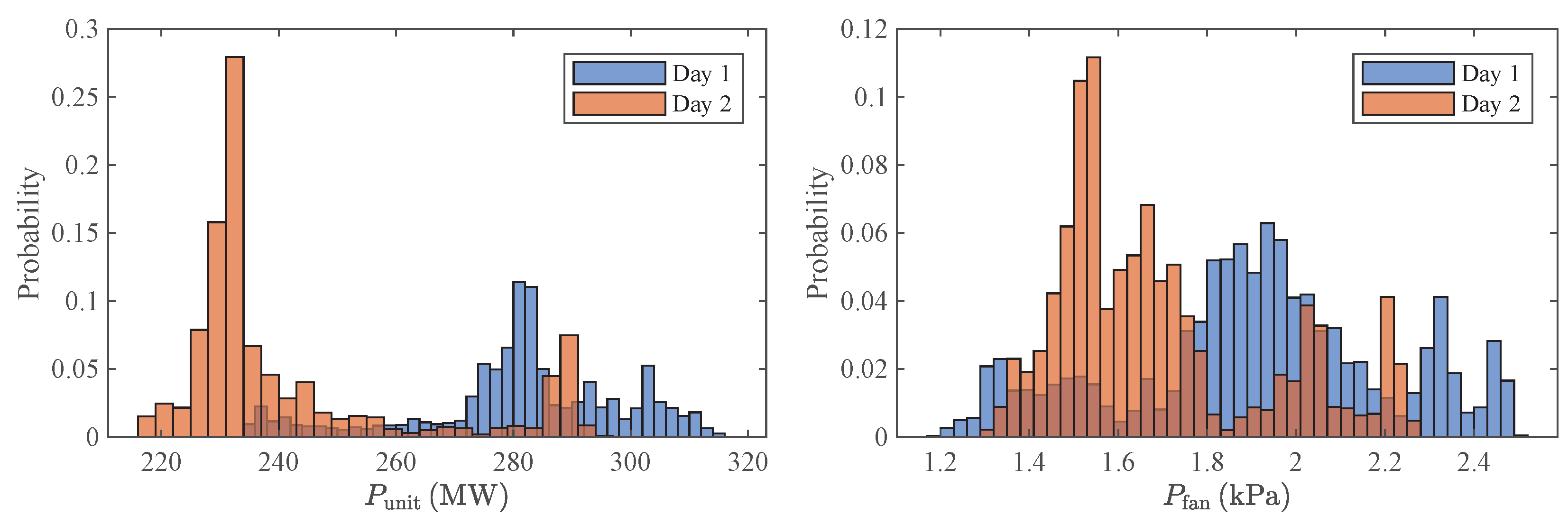
The data from two different day are extracted to illustrate the distribution shift under varying operating conditions. The histogram of the unit power $P_{\mathrm{unit}}$ and the output pressure $P_{\mathrm{fan}}$ is generated using MATLAB R2023a and presented in Figure 1. There are obviously significant differences in the data distribution between these two days. Traditional data-driven approaches can maintain good performance when the training dataset and the test dataset have the same or similar data distribution. However, for the data shown in Figure 1, the model built based on the data on Day 1 may not perform well on Day 2. If a data-driven model exhibits poor fitting performance, model residual-based operation monitoring methods are likely to fail. Consequently, the monitoring indicator may persistently exceed the alarm threshold even under normal operation conditions, leading to frequent false alarms. Even though a data-driven model exhibits good fitting performance, transient disturbances or sensor noise may also cause false alarms. A post-processing mechanism is required to reduce these false alarms.

3.2. Overall Framework

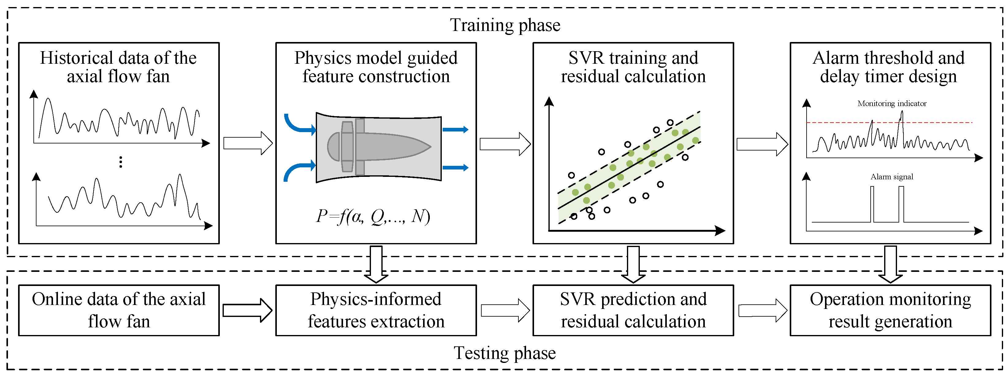
An operation monitoring method for axial flow fans based on physics-guided support vector regression and alarm delay timer is proposed. The overall framework of the proposed method is prepared using Microsoft Visio and depicted in Figure 2. The framework consists of an offline training phase and an online monitoring phase. The historical and online data used in the proposed framework are acquired from the same DCS system described in Section 3.1. In the offline phase, historical data of raw process variables are collected. The physical model of the axial flow fan is developed based on blade aerodynamics. The physically augmented features are constructed under the guidance of the physical model. The support vector regression model is trained on the basis of physically augmented features for fan pressure prediction. Model residuals are computed as the monitoring indicator on the training dataset to determine the alarm threshold. The alarm duration is calculated to discover the characteristics of false alarm events. The delay factor of the alarm delay timer is designed through the analysis of the alarm duration.

In the online phase, real-time measurements of process variables are processed through the same physical feature augmentation. The fan pressure is predicted by the trained support vector regression model. The model output is compared with the actual fan pressure to compute the model residual. The change in the model residual indicates the operating condition of the axial flow fan. If the model residual exceeds the designed alarm threshold and lasts longer than the delay factor of the alarm delay timer, then an alarm is triggered. The proposed operation monitoring framework has two advantages. First, the proposed physics-guided feature construction method integrates physical knowledge of the axial flow fan into the data-driven model. The physics-guided support vector regression model shows better interpretability and generalization. Second, the alarm duration is introduced to mine the characteristics of false alarm events caused by transient disturbances. The designed alarm delay timer effectively reduces false alarms while maintaining high sensitivity to abnormal conditions.

4. Methodology

This section presents the proposed method in detail, including the physics-guided feature construction, the support vector regression, and the alarm delay timer.

4.1. Physics-Guided Feature Construction

Raw process variables and derived features form the foundation of data-driven models. The proposed physical feature augmentation method selects raw process variables and extracts physically augmented features guided by the physical model of axial flow fans. The augmented features carry explicit physical meanings. Consequently, the data-driven model established with augmented features offers enhanced interpretability compared with models established with raw process variables. The physical model is the core of the physics-based feature augmentation method. The physical model of axial flow fans can be derived from the Euler equation [28]. The theoretical head per unit mass of fluid, denoted as $H_0$ (in meters), for the axial flow fan is

$$H_0={\displaystyle \frac{1}{g}}u{c}_2,$$

(1)

where g (in m/s²) is the acceleration of gravity, u (in m/s) is the circular velocity of the impeller, and $c_2$ (in m/s) is the circumferential component of the absolute velocity at the impeller outlet. The theoretical total pressure $P_0$ (in Pa) of the axial flow fan under ideal assumptions of inviscid, incompressible, and steady flow is expressed as

$$P_0=\rho g{H}_0=\rho u{c}_2,$$

(2)

where $\rho$ (in kg/m³) is the fluid density. The circumferential component of the absolute velocity $c_2$ can be obtained by velocity vector decomposition

$$c_2=u-v\cot \beta ,$$

(3)

where $\beta$ (in degrees) is the blade angle, which can be derived from the fan blade position feedback ${\alpha }_{\mathrm{fan}}$ measured in the industrial field. And v (in m/s) is the axial component of the absolute velocity. The axial velocity v is expressed as

$$v={\displaystyle \frac{Q}{A}},$$

(4)

where Q (in m³/s) is the flow rate, and A (in m²) is the cross-sectional flow area. The theoretical total pressure $P_0$ can be obtained by substituting Equation (3) into Equation (2),

$$P_0=\rho u^2-\rho u{\displaystyle \frac{Q}{A}}\cot \beta .$$

(5)

The circular velocity of the impeller u is given by

$$u={\displaystyle \frac{2\pi N}{60}}r,$$

(6)

where r (in m) is the impeller radius, and N (in r/min) is the rotational speed. For an axial flow fan with adjustable blades, the rotation speed N is typically treated as a constant value. In axial flow fans, pressure losses such as frictional loss $\Delta P_{\mathrm{f}}$ (in Pa) and incidence loss $\Delta P_{\mathrm{i}}$ (in Pa) are present. The actual fan pressure P (in Pa) is equal to the theoretical total pressure $P_0$ minus these pressure losses:

$$P=P_0-\Delta P_{\mathrm{f}}-\Delta P_{\mathrm{i}},$$

(7)

where $\Delta P_{\mathrm{f}}$ is roughly proportional to the square of the flow rate

$$\Delta P_{\mathrm{f}}=K_{\mathrm{f}}\left(\beta \right)Q^2.$$

(8)

The frictional loss coefficient $K_{\mathrm{f}}\left(\beta \right)$ is a function of the blade angle $\beta$. The incidence loss $\Delta P_{\mathrm{i}}$ is expressed as

$$\Delta P_{\mathrm{i}}=K_{\mathrm{i}}\left(\beta \right){(Q-Q_{\mathrm{d}}\left(\beta \right))}^2,$$

(9)

where $Q_{\mathrm{d}}\left(\beta \right)$ is the designed flow rate under the blade angle $\beta$. The incidence loss coefficient $K_{\mathrm{i}}\left(\beta \right)$ is also a function of the blade angle $\beta$. Considering the process variables available in industrial fields, the physical model of the axial flow fan can be simplified as

$$P=k_1\left(\beta \right)-k_2\left(\beta Q\right)-k_3\left(\beta Q^2\right),$$

(10)

where

$$k_1\left(\beta \right)=\rho u^2-K_{\mathrm{i}}\left(\beta \right)Q_{\mathrm{d}}{\left(\beta \right)}^2,$$

(11)

$$k_2\left(\beta Q\right)=2K_{\mathrm{i}}\left(\beta \right)Q_{\mathrm{d}}\left(\beta \right)Q-{\displaystyle \frac{\rho uQ\cot \beta }{A}},$$

(12)

$$k_3\left(\beta Q^2\right)=-K_{\mathrm{f}}\left(\beta \right)Q^2-K_{\mathrm{i}}\left(\beta \right)Q^2.$$

(13)

Some model parameters, such as the rotational speed N and flow area A, can be derived from operating procedures. In contrast, other parameters, such as frictional loss coefficient $K_{\mathrm{f}}\left(\beta \right)$ and incidence loss coefficient $K_{\mathrm{i}}\left(\beta \right)$, are not available in practice. The availability of these model parameters is not a prerequisite. The proposed method utilizes their structural forms to guide the construction of augmented features. Data-driven models are then utilized to approximate these known or unknown model parameters. Based on Equation (10), the augmented features such as $\beta$, $\beta Q$, and $\beta Q^2$, can be constructed for data-driven modeling. The physical model of axial flow fan is derived from fundamental laws of conservation. The physical model naturally possesses inherent generalization capability across varying operating conditions. This inherent generalization capability is the key to addressing the distribution shifts across operating days. The features constructed under the guidance of the physical model inherit this generalization capability. The idea of physics-guided feature construction is conceptually related to invariant representation learning across different domains in domain generalization. The physically augmented features in the proposed method fulfill the same objective through explicit physics-based construction instead of data-driven representation learning.

4.2. Support Vector Regression

The support vector regression is kernel-based learning method with a solid scientific foundation in statistical learning theory. The core principle is structural risk minimization, which balances empirical error and model complexity to achieve good generalization. The support vector regression employs the kernel trick to implicitly constructs high-dimensional features from the input space. The choice of kernel function is based on the established physical model of the axial flow fan. With these physically augmented features constructed in Section 4.1, the support vector regression is established for fan pressure modeling. The input feature vector is defined as $x=[\beta ,\beta Q,\beta Q^2]$, and the output is the actual fan pressure P. The support vector regression model aims to find the optimal regression hyperplane for the data samples to make the model output as close as possible to the actual values

$$g\left(x\right)={\phi }^{\top }x+b,$$

(14)

where $g\left(x\right)$ is the output of the support vector regression, $\phi$ is the weight, and b is the bias. The support vector regression allows for a certain degree of deviation between the model output and the actual values [29,30]. The calculation of the model loss only begins when the absolute value of the error exceeds $\tau$. The optimization problem can be obtained

$$\begin{array}{c}\underset{\phi ,b}{min}{\displaystyle \frac{1}{2}}{\phi }^2+\Psi {\displaystyle \sum _{i=1}^L}{\xi }_i,\hfill \\ s.t.\left\{\begin{array}{c}{y}_i-{\phi }^{\top }{x}_i-b\le \tau +{\xi }_i\\ {\phi }^{\top }{x}_i+b-y_i\le \tau +{{\xi }^{*}}_i\\ {\xi }_i\ge 0,{{\xi }^{*}}_i\ge 0\end{array}\right.,\hfill \end{array}$$

(15)

where $\Psi$ is the penalty coefficient, ${\xi }_i$ and ${{\xi }^{*}}_i$ are slack variables. The loss function is transformed into

$$l\left(\vartheta \right)=\left\{\begin{array}{cc}0,& \left|\vartheta \right|\le \tau \\ \left|\vartheta \right|-\tau ,& \left|\vartheta \right|>\tau \end{array}\right..$$

(16)

The model output error will not be included in the loss function when the training data falls within the range of $[-\tau ,\tau ]$. If the training data falls outside the range, the model output error after subtracting will be included in the loss function. The optimization problem can be solved by introducing the Lagrange term

$$g\left(x\right)={\displaystyle \sum _{i=1}^L}\left({\lambda }_i-{\lambda }_i^{*}\right)\left(x·x_i\right)+b.$$

(17)

The support vector regression introduces the kernel function for nonlinear problem. The training data is mapped into a high-dimensional feature space,

$$g\left(x\right)={\displaystyle \sum _{i=1}^L}\left({\lambda }_i-{\lambda }_i^{*}\right)\psi \left(x_i,x\right)+b,$$

(18)

where $\psi \left(·\right)$ is the kernel function. Two kernel functions are used for the support vector regression, including the linear kernel and the polynomial kernel

$${\psi }_{\mathrm{lin}}\left(x_i,x_j\right)={x_i}^{\top }{x}_j,$$

(19)

$${\psi }_{\mathrm{poly}}\left(x_i,x_j\right)={({x_i}^{\top }{x}_j+c)}^d,$$

(20)

where d is the polynomial order of the polynomial kernel. The choice of kernel functions is guided by the physical model structure developed in Section 4.1. The physical model presented in Equation (10) indicates an approximately linear or low-order polynomial relationship between the fan pressure and the constructed features. The linear kernel naturally aligns with the approximately linear structure of the physical model. The low-degree polynomial kernel is also considered to account for potential mild nonlinearities that may arise from simplifications in the physical model. The radial basis function kernel is excluded because it introduces excessive complexity without physical justification. The physical model already provides a underlying physical structure. The application of the radial basis function kernel would lack consistency with the known physical structure, and may impair the generalization capability that the physics-guided features can provide.

4.3. Alarm Delay Timer

The model residual is adopted as the monitoring indicator for detecting the abnormal condition of axial flow fans. The principle of model residual-based monitoring is that when an abnormality such as stall or surge occurs, the aerodynamics of axial flow fans deviate from the normal condition, leading to a significant increase in the model residual. The model residual-based monitoring strategy has two advantages. First, the measured fan pressure by a sensor alone is not a reliable indicator for operation monitoring. The fan pressure varies significantly with the change of operating conditions. A fixed threshold on the fan pressure is unable to discriminate between normal load changes and abnormal conditions. Unlike the conventional monitoring strategy, the residual-based monitoring strategy uses the residual to depict the deviation from expected behavior under the current operating conditions. The residual provides a more reliable indicator for operation monitoring by removing the influence of normal condition variations. Second, abnormal events such as stall or surge are rare in industrial practice, and the collection of sufficient fault data is often impractical [31]. The residual-based monitoring strategy develops a model to capture the fan behavior under normal conditions. The training process of the model only requires normal data. This makes the residual-based monitoring strategy particularly suitable for industrial applications where fault data are scarce.

The model residual is defined as the Euclidean distance between the actual fan pressures and predicted fan pressures

$$h=|P-\widehat{P}|,$$

(21)

where h is the monitoring indicator of the axial flow fan, P is the actual fan pressure, and $\widehat{P}$ is the predicted fan pressure by the support vector regression model. Under normal conditions, the monitoring indicator h is supposed to be small. When an abnormal condition occurs, h increases significantly to indicate a potential fault. The alarm threshold $h_{\mathrm{th}}$ is determined systematically from the residual distribution under normal operating conditions. The procedure consist of two steps. In the first step, the probability density function $p\left(h\right)$ of the residual h is obtained from historical normal data using kernel density estimation as

$$\widehat{p}\left(h\right)={\displaystyle \frac{1}{n}}{\displaystyle \sum _{i=1}^n}{K}_{\sigma }(h-h_i),$$

(22)

where $h_i$’s are the residual samples under normal conditions, $K_{\sigma }(·)$ is a Gaussian kernel function, and $\sigma$ is the bandwidth parameter. In the second step, given a preset confidence level $\eta$, the alarm threshold $h_{\mathrm{th}}$ is computed as the $(1-\eta )\times 100\%$ quantile of the estimated cumulative distribution function,

$${\int }_0^{h_{\mathrm{th}}}\widehat{p}\left(h\right)\mathrm{d}h=\eta .$$

(23)

A higher $\eta$ yields a higher threshold and thus a lower false alarm rate, while a lower $\eta$ results in a more sensitive but more easily triggered alarm threshold. If the monitoring indicator h exceeds the alarm threshold $h_{\mathrm{th}}$, the alarm signal will be triggered, and the axial flow fan is considered to be in the abnormal condition. However, transient disturbances or sensor noise may cause transient residual peaks, leading to frequent false alarms. A post-processing mechanism is required to reduce these false alarms. To reduce false alarms caused by transient residual spikes, the alarm delay timer is designed as a post-processing module. The alarm delay timer is a powerful tool that has been applied in various industrial fields. The principle of the alarm delay timer is that an alarm signal only raises when the monitoring indicator h exceeds the alarm threshold $h_{\mathrm{th}}$ and lasts for a period of time [32]. The design of the alarm delay timer is as follows. Let y denote the original alarm signal that can be derived from the comparison between the monitoring indicator and the alarm threshold

$$y\left(t\right)=\left\{\begin{array}{c}1,\mathrm{if}h\left(t\right)\ge h_{\mathrm{th}}\hfill \\ 0,\mathrm{otherwise},\hfill \end{array}\right.$$

(24)

where $y\left(t\right)$ is the value of the original alarm signal at time t, and $h\left(t\right)$ is the value of the monitoring indicator at time t. The form of the alarm delay timer can be expressed as

$$\begin{array}{cc}\hfill y_{\mathrm{d}}\left(t\right)& =\left\{\begin{array}{cc}1,\hfill & \begin{array}{cc}\mathrm{if}\hfill & y_{\mathrm{d}}(t-1)=0\hfill \\ \hfill & \&{\sum }_{i=t-m+1}^{t}y\left(t\right)=m\hfill \end{array}\hfill \\ 0,\hfill & \begin{array}{cc}\mathrm{if}\hfill & y_{\mathrm{d}}(t-1)=1\hfill \\ \hfill & \&{\sum }_{i=t-m+1}^{t}y\left(t\right)=0\hfill \end{array}\hfill \\ y_{\mathrm{d}}(t-1),\hfill & \mathrm{otherwise},\hfill \end{array}\right.\hfill \end{array}$$

(25)

where $y_{\mathrm{d}}\left(t\right)$ is the value of the alarm signal processed by the alarm delay timer at time t, and m is the delay factor of the alarm delay timer. The delay factor of the alarm delay timer can be determined based on the alarm duration of alarm events. The alarm duration is the duration time from the trigger of an alarm to the clearance of the alarm in an alarm event. The alarm delay timer with a delay factor m can eliminate false alarms with the alarm duration less than m. The false alarm ratio $\chi \left(m\right)$ is defined as the ratio of remaining false alarms $F\left(m\right)$ to the total number of false alarms $F_0$ with the use of the alarm delay timer with a delay factor m,

$$\chi \left(m\right)={\displaystyle \frac{F\left(m\right)}{F_0}},$$

(26)

where $F_0$ is the total number of false alarms. Given a desired false alarm ratio ${\chi }_0$, the design of the delay factor can be regarded as an optimization problem

$$m_{\mathrm{opt}}=arg\underset{m}{min}|\chi \left(m\right)-{\chi }_0|.$$

(27)

The solution of this optimization problem can be derived from the probability distribution of alarm durations [33]. The alarm duration $T\left(j\right)$ is defined as the time duration of the j-th alarm event

$$T\left(j\right)=t_{\mathrm{c}}\left(j\right)-t_{\mathrm{o}}\left(j\right)+1,$$

(28)

where $t_{\mathrm{o}}\left(j\right)$ is the time instant of alarm occurrence for the j-th alarm event, and $t_{\mathrm{c}}\left(j\right)$ is the time instant of alarm clearance for the j-th alarm event. The Bayesian approach is applied to obtain a reliable estimate of the probability density function of alarm duration. The prior probability density function of the alarm duration is treated as a continuous uniform distribution

$$p_{{\Gamma }_k}\left({\gamma }_k\right)=\left\{\begin{array}{cc}1,\hfill & 0<{\gamma }_k<1\hfill \\ 0,\hfill & \mathrm{otherwise}\hfill \end{array}\right..$$

(29)

Let $M_K$ be a discrete random variable taking a sample $M_k$, which is the number of alarm events that satisfy $T\left(j\right)=k$ in the dataset. Since each alarm duration is associated with an independent alarm event, $M_K$ follows a binominal distribution

$$p_{M_K\mid {\Gamma }_k}(M_k\mid {\gamma }_k)={\displaystyle \frac{M!}{M_k!(M-M_k)!}}·{\gamma }_k^{M_k}·{(1-{\gamma }_k)}^{M-M_k}.$$

(30)

The joint probability distribution of $M_k$ and ${\Gamma }_k$ can be calculated as

$$p_{M_K,{\Gamma }_k}(M_k,{\gamma }_k)=p_{M_k\mid {\Gamma }_k}(M_k\mid {\gamma }_k)·p_{{\Gamma }_k}\left({\gamma }_k\right).$$

(31)

The posterior probability distribution of ${\Gamma }_k$ is

$$p_{{\Gamma }_k\mid M_K}({\gamma }_k\mid M_k)={\displaystyle \frac{p_{M_K,{\Gamma }_k}(M_k,{\gamma }_k)}{p_{M_K}\left(M_k\right)}}={\displaystyle \frac{p_{M_K,{\Gamma }_k}(M_k,{\gamma }_k)}{\int p_{M_K,{\gamma }_k}(M_k,{\gamma }_k)\mathrm{d}{\gamma }_k}}.$$

(32)

The Bayesian estimate is regarded as the conditional mean of ${\Gamma }_k$ is

$${\widehat{\gamma }}_k=\int {\gamma }_k·p_{{\Gamma }_k\mid M_K}({\gamma }_k\mid M_k)\mathrm{d}{\gamma }_k.$$

(33)

If the conditional mean ${\widehat{\gamma }}_k$ is large with respect to the confidence interval, then ${\widehat{\gamma }}_k$ can be taken as a reliable estimate of ${\Gamma }_k$. Once the delay factor $m_{\mathrm{opt}}$ is determined, the alarm threshold $h_{\mathrm{th}}$ and the alarm delay timer are utilized for operation monitoring.

5. Experiment and Discussions

This section describes the experimental setup and presents the results in detail to illustrate the effectiveness of the proposed method.

5.1. Experimental Setup

The data used for experiments are acquired from the DCS system of a 300 MW coal-fired thermal power plant. The data processing and visualization are performed in MATLAB R2023a to prepare all tables and figures in Section 5. The data are collected from an axial flow fan in a 300 MW thermal power plant in Shandong Province for experiments. The type of the axial flow fan is FAF25-12.5-1, which is made by the Shanghai Electric Blower Works Co., Ltd, Shanghai, China. The sampling interval of the data is 1 s. The process variables related to the axial flow fan are listed in Table 1. The training dataset and four test datasets are collected on different days to evaluate the fitting performance of the regression models. The training dataset contains 40,000 samples, and each test dataset contains 20,000 samples. In addition, a separate fan stall case is utilized to illustrate the effectiveness of the alarm delay timer and the monitoring performance.

Two types of input features are considered. The first type consists of the raw process variables. The second type comprises the augmented features derived from the physical model presented in Section 4.1. Four regression models are trained and compared for fan pressure prediction. The support vector regression with a linear kernel using raw process variables is denoted as SVR-L, while the version using augmented features is denoted as SVR-L-A. Similarly, the support vector regression with a polynomial kernel trained with raw process variables is denoted as SVR-P, and its counterpart trained with augmented features is denoted as SVR-P-A. Considering the physical model presented in Equation (10), the polynomial order d for the polynomial kernel is set to 2. The grid search is used to determine the hyperparameters for training these four support vector regression models. The search range of the hyperparamters in the grid research is $\Psi , \tau \in \{{10}^{-3},{10}^{-2},{10}^{-1},1,10,{10}^2,{10}^3\}$. The maximum number of iterations is set to ${10}^5$. The confidence level $\eta$ is set to 0.99 to determine the alarm threshold $h_{\mathrm{th}}$. The desired false alarm ratio ${\chi }_0$ is set to 0.05 to determine the delay factor m of the alarm delay timer. The coefficient of determination ${\mathrm{R}}^2$ and root mean square error $\mathrm{RMSE}$ are adopted to evaluate the fitting performance of regression models. The number of false alarms $N_{\mathrm{F}}$ and missed alarms $N_{\mathrm{M}}$ are computed to evaluate the overall monitoring performance.

5.2. Result Analysis

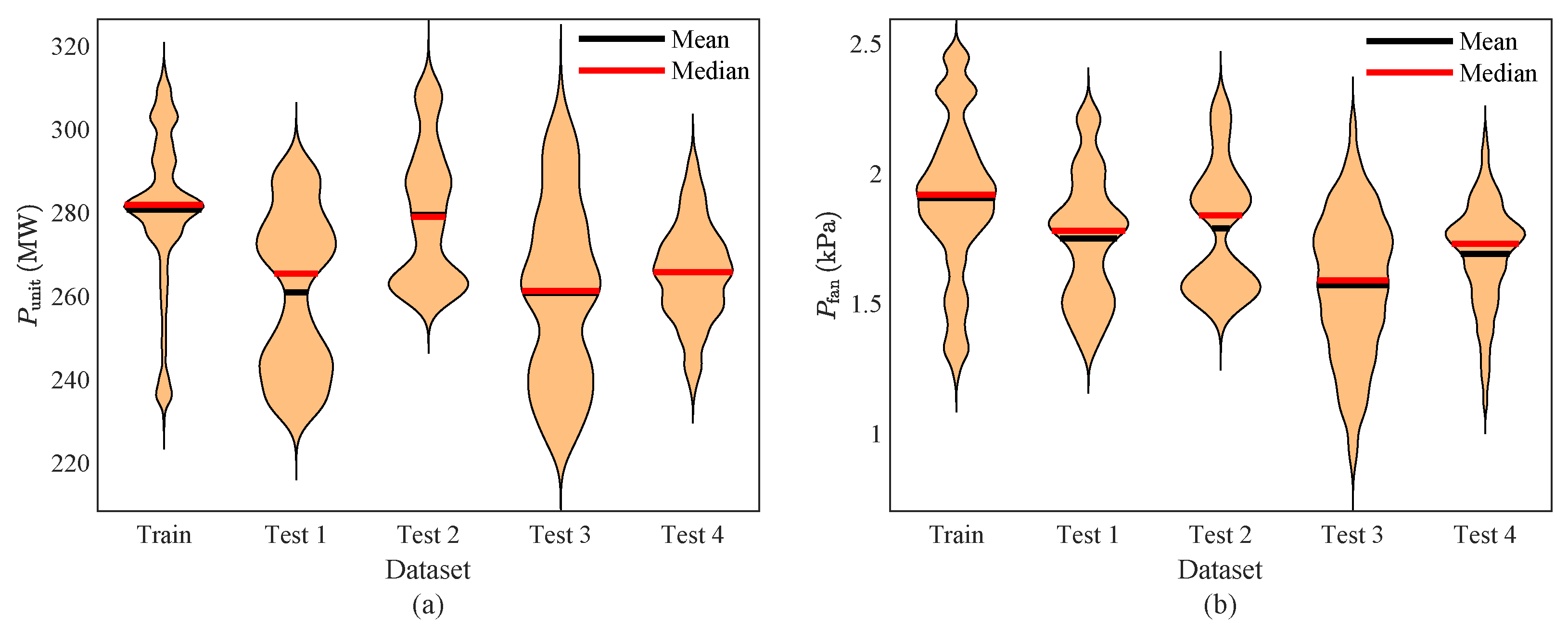
The violin plot presented in Figure 3 reveals the distribution of $P_{\mathrm{unit}}$ and $P_{\mathrm{fan}}$ across the training dataset and four test datasets. As shown in Figure 3a, the training dataset exhibits a relatively concentrated distribution with a median value around 280 MW for $P_{\mathrm{unit}}$. The four test datasets show varying degrees of dispersion in $P_{\mathrm{unit}}$. It reveals the natural variability of operating conditions across different days for the thermal power unit. Both the training dataset and four test datasets are collected under normal operation conditions. These distribution shifts are not due to equipment faults but reflect normal day-to-day variations in load demand and ambient conditions. The variations of $P_{\mathrm{unit}}$ result in the variations of $P_{\mathrm{fan}}$, like shown in Figure 3b. Consequently, the test datasets contain operating conditions not fully covered by the training dataset. These training and test datasets represent a realistic and challenging scenario for evaluating model generalization.

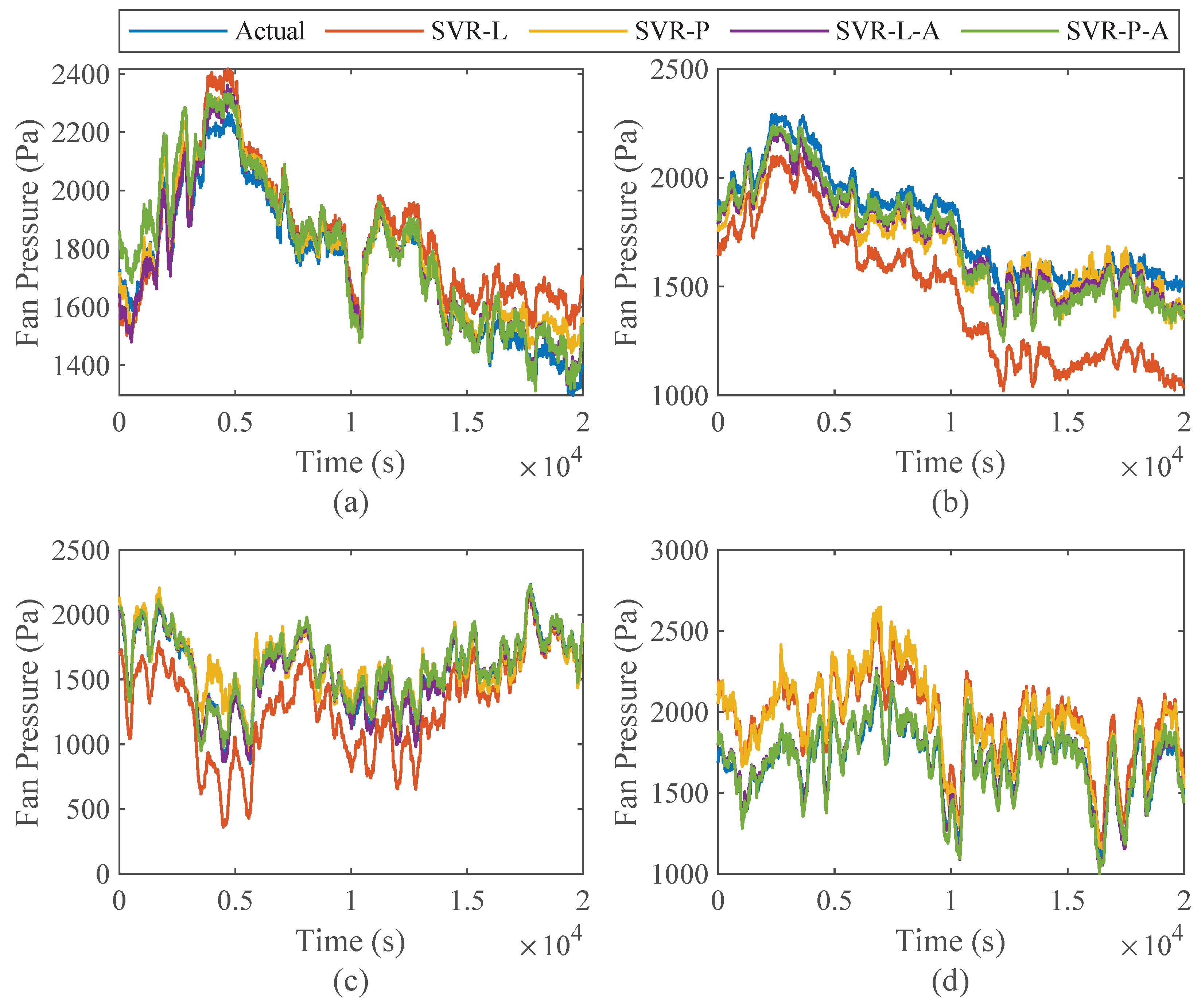
The fitting performance of the four SVR models on the training and four test datasets are summarized in

Table 2. Fitting performance of four SVR models on training and test datasets.

Model	Metric	Train	Test 1	Test 2	Test 3	Test 4
SVR-P	RMSE	21.4880	65.9434	101.6189	111.3588	280.5623
	${\mathrm{R}}^2$	0.9948	0.9257	0.8178	0.8348	−0.9772
SVR-L	RMSE	42.9684	122.5639	334.1309	303.4651	272.6947
	${\mathrm{R}}^2$	0.9794	0.7432	−0.9696	−0.2272	−0.8679
SVR-P-A	RMSE	40.2398	73.3162	92.7318	66.8220	53.7517
	${\mathrm{R}}^2$	0.9819	0.9081	0.8483	0.9405	0.9274
SVR-L-A	RMSE	45.8317	53.0947	88.7582	43.4324	50.2274
	${\mathrm{R}}^2$	0.9766	0.9518	0.8610	0.9749	0.9366

. On the training dataset, all models achieve high accuracy, with ${\mathrm{R}}^2$ values ranging from 0.9766 to 0.9948 and $\mathrm{RMSE}$ values from 21.4880 to 45.8317. However, the performance varies significantly across models on the test datasets. SVR-L and SVR-P, which use raw process variables, exhibit severe performance degradation on test datasets. For instance, SVR-L yields an ${\mathrm{R}}^2$ of −0.9696 and an $\mathrm{RMSE}$ of 334.13 on the Test 2 dataset. And SVR-P gives an ${\mathrm{R}}^2$ of −0.9772 and an $\mathrm{RMSE}$ of 280.56 on the Test 4 dataset. These negative ${\mathrm{R}}^2$ values indicate that the models fail to capture the underlying data patterns. As shown in Figure 4b, the output values of SVR-L (orange line) evidently deviate the actual values of the fan pressure (blue line). In contrast, the models using augmented features, SVR-L-A and SVR-P-A, show better generalization. SVR-L-A achieves the best overall fitting performance, with ${\mathrm{R}}^2$ values of 0.9518 on Test 1, 0.8610 on Test 2, 0.9749 on Test 3, and 0.9366 on Test 4, accompanied by relatively low $\mathrm{RMSE}$ values. SVR-P-A also maintains stable performance across all test datasets, with ${\mathrm{R}}^2$ values consistently above 0.84. Among all models, SVR-L-A is the most robust model and is selected for further operation monitoring.

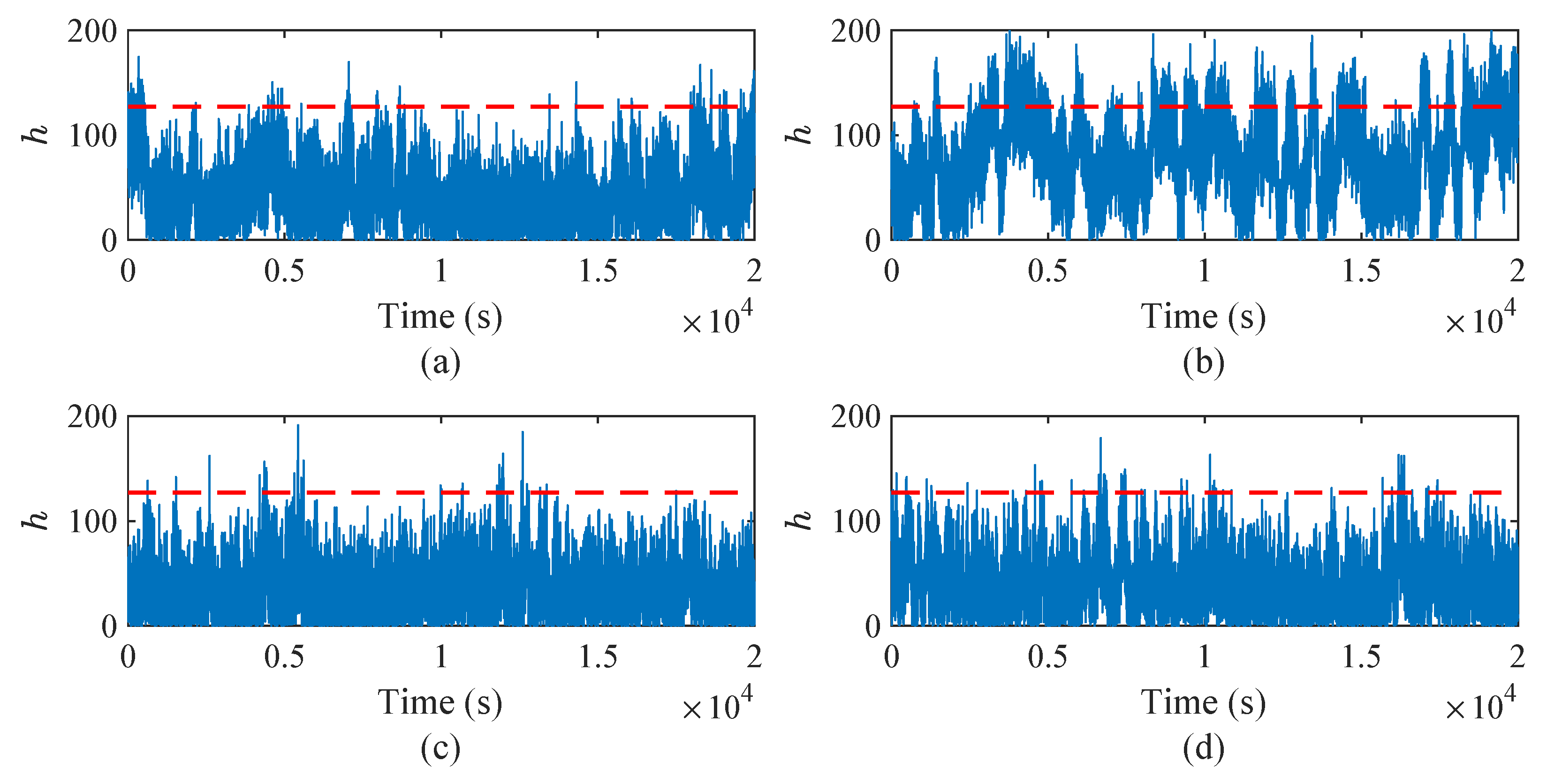
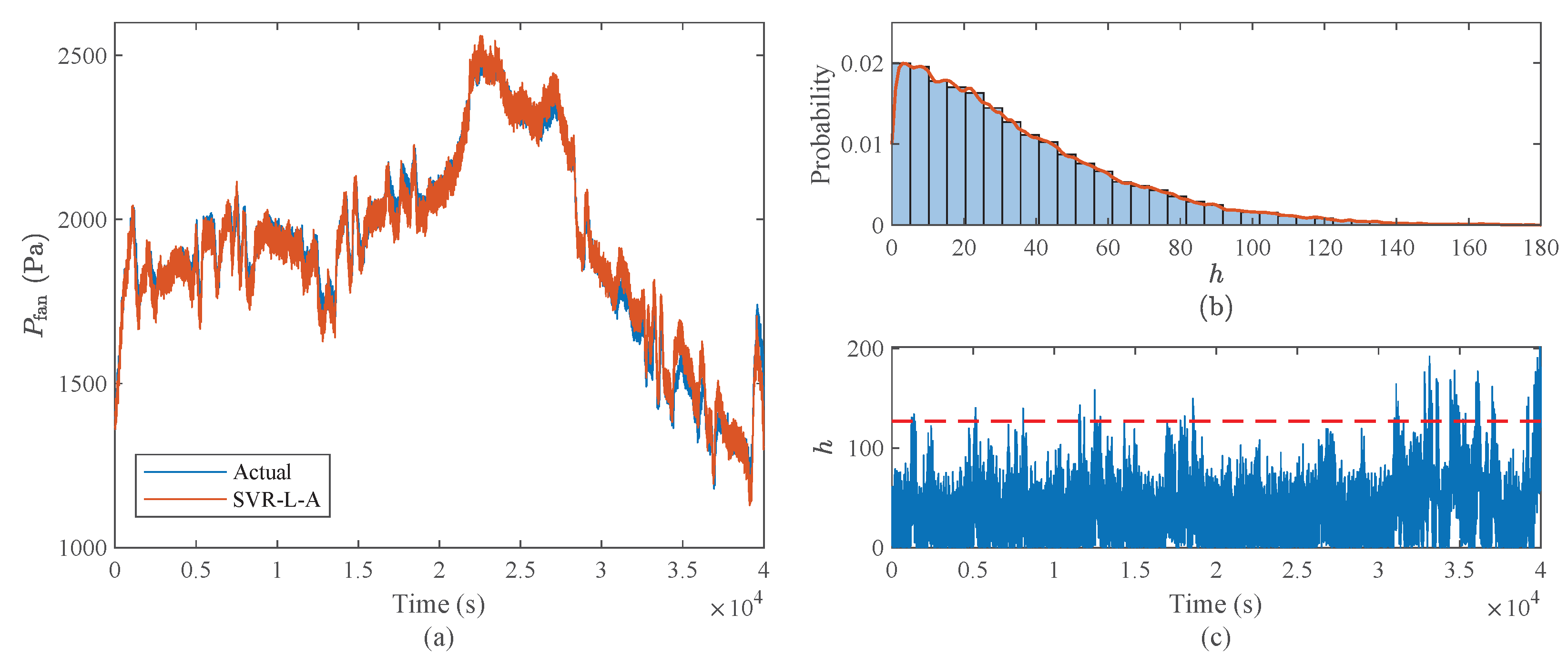
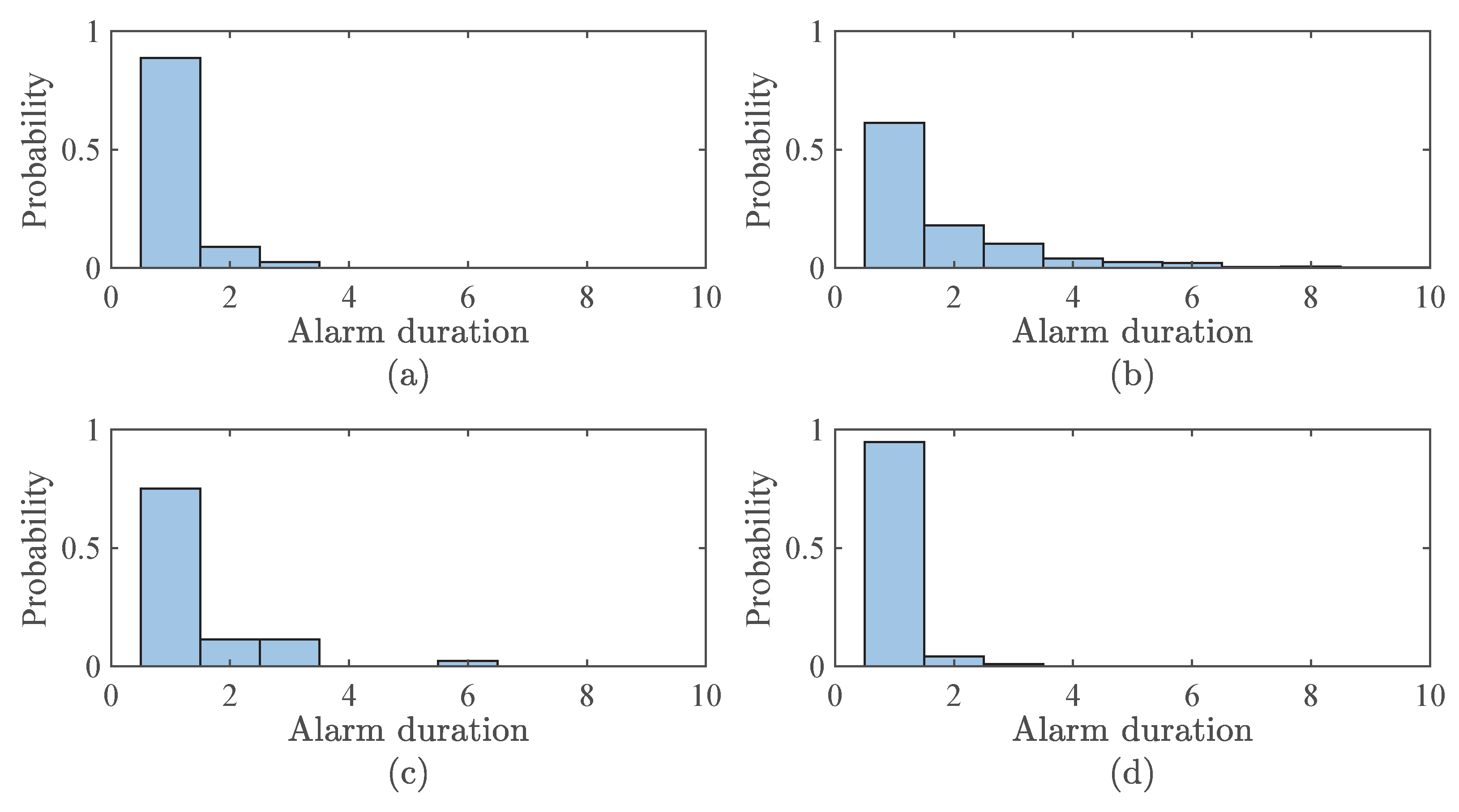
The fitting results of SVR-L-A on the training dataset is presented in Figure 5a. The Euclidean distance between the actual values of fan pressures and the outputs of SVR-L-A is calculated as the monitoring indicator. The histogram of the monitoring indicator on the training dataset is depicted in Figure 5b. The alarm threshold is designed as $h_{\mathrm{th}}=127.0597$ based on the confidence level $\eta$. The change of the monitoring indicator on the training dataset is shown in Figure 5c. Although SVR-L-A has good fitting performance on the training dataset, there still exist 271 false alarms caused by transient disturbances. The changes in the monitoring indicator on the four test datasets are demonstrated in Figure 6. There are also varying degrees of false alarms in the four test datasets. The number of false alarms in the four test datasets are 123, 1314, 44, and 95 respectively. The alarm delay timer is designed to reduce false alarms. The alarm duration is computed to describe the characteristics of these false alarm events. The histogram of the alarm duration on the four test datasets is presented in Figure 7. The alarm durations of all false alarm events in Test 1 and Test 4 dataset persist within 3 s. In Test 2 dataset, over 95% of false alarm events last less than 5 s. And over 95% false alarm events in Test 3 dataset remain within 3 s. It is evident that the alarm duration of these false alarm events are short. The alarm delay timer is appropriate for the reduction of false alarms. The alarm durations of all false alarm events on the four test datasets are summarized, and the delay factor of the alarm delay timer is designed as $m_{\mathrm{opt}}=5$. The alarm threshold and the alarm delay timer are utilized for operation monitoring for the axial flow fan.

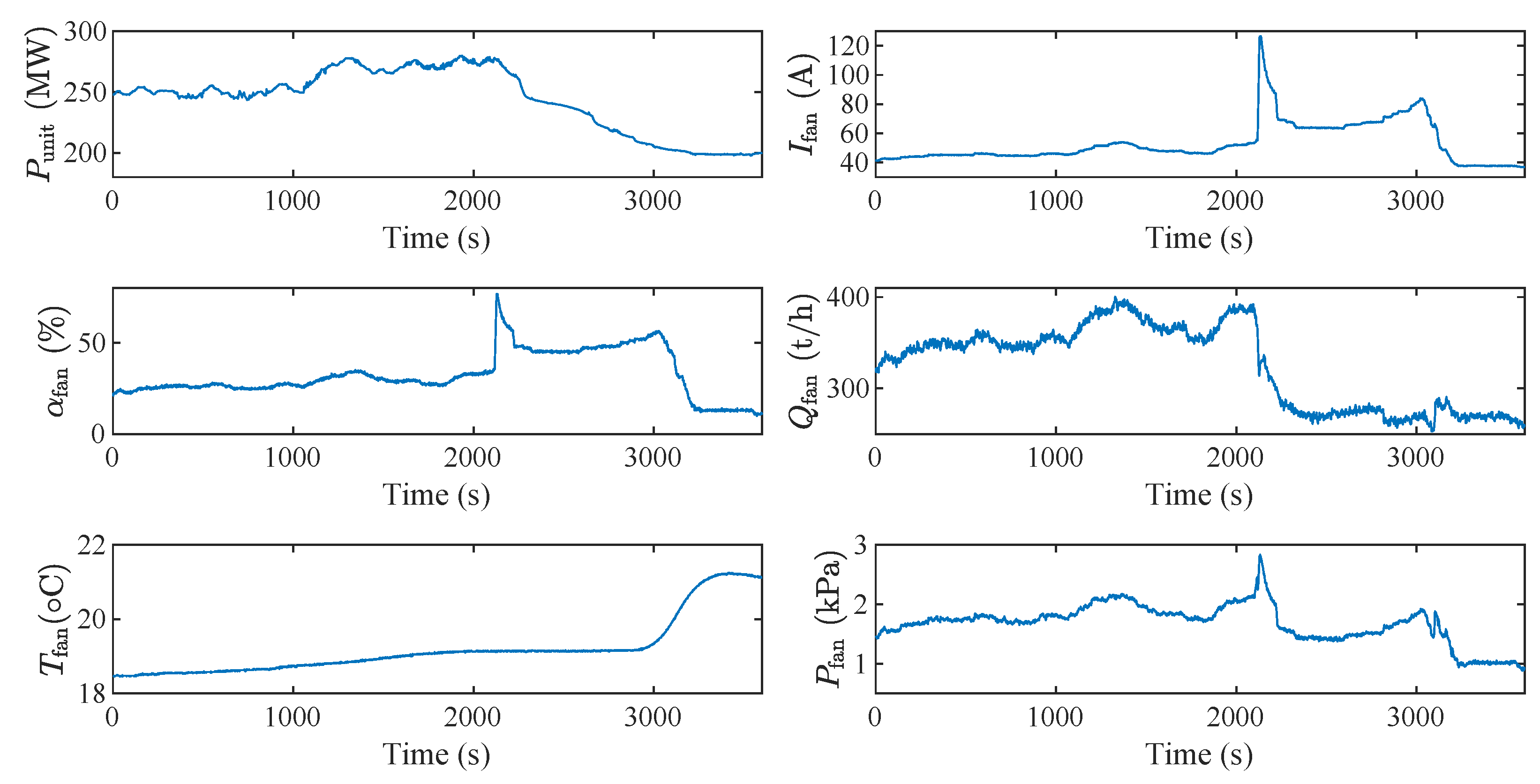
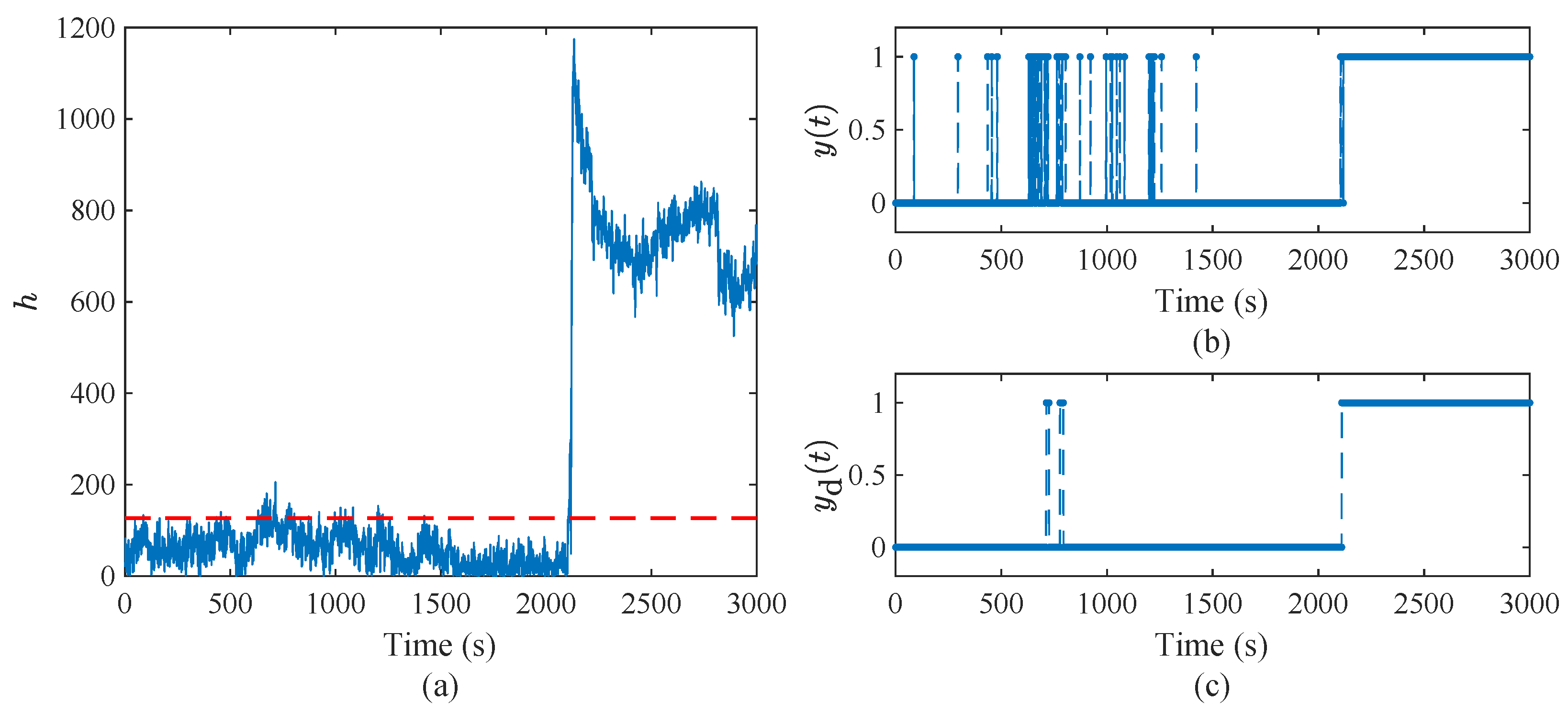
A separate fan stall case is used to support the proposed method. The changes in related process variables in the fan stall case are shown in Figure 8. Some process variables, such as the blade position feedback and output pressure, show abnormal fluctuations at about 2103 s during the fan stall condition. The change in the monitoring indicator for the fan stall case is demonstrated in Figure 9a. The monitoring indicator significantly exceeds the alarm threshold at about 2107 s, and the alarm signal is triggered. The operating condition of the axial flow fan is identified as abnormal. However, the monitoring indicator has transient peaks under normal condition caused by noises and disturbances, leading to exceed the alarm threshold and false alarms. The original alarm signal $y\left(t\right)$ for the fan stall case are illustrated in Figure 9b. It is apparent that the original alarm signal has a lot of false alarms in normal operating condition. The alarm signal $y_{\mathrm{d}}\left(t\right)$ processed by the alarm delay timer is depicted in Figure 9c. With the use of the designed alarm delay timer, the number of false alarms is reduced from 43 to 2, and missed alarms decrease from 2 to 0. The detection delay increased from 4 s to 8 s since the alarm delay timer introduces a time window to confirm that the monitoring indicator persistently exceeds the alarm threshold. The detection delay remains within an acceptable range for practical industrial applications. The substantial reduction in false alarms significantly improves system reliability. The monitoring performance of different models for this fan stall case is illustrated in

Table 3. Performance comparison of different models in terms of $N_{\mathrm{F}}$ and $N_{\mathrm{M}}$ for the fan stall case.

	SVR-P	SVR-L	SVR-P-A	SVR-L-A	SVR-L-A + Delay Timer
$N_{\mathrm{F}}$	93	136	53	43	2
$N_{\mathrm{M}}$	0	1	0	2	0

. The SVR-P yields 93 false alarms without missed alarms. The SVR-L produces 136 false alarms and 1 missed alarm. With the physics-guided features, the SVR-P-A generates 53 false alarms without missed alarms, while the SVR-L-A shows 43 false alarms and 2 missed alarms. The SVR-L-A with the alarm delay timer achieves 2 false alarms without missed alarms. The use of the alarm delay timer can effectively reduce false alarms and maintain the detection ability of abnormal conditions.

5.3. Discussion

The training dataset and four test datasets in this study were collected across different operating days. The violin plots presented in Figure 3 indicate that the unit power $P_{\mathrm{unit}}$ and fan pressure $P_{\mathrm{fan}}$ vary considerably from day to day. This day-to-day variation reflects the distribution shift caused by changing load conditions in industrial practice, which is the central challenge addressed in this study. The proposed method is designed to achieve reliable fan modeling and monitoring performance under varying load conditions. The experiment results across these datasets from distinct operating days provide direct evidence of its effectiveness. Table 2 compares the fitting performance of four models on the training and four test datasets. The results demonstrate the effectiveness of physics-guided features in improving model generalization. The SVR-L exhibits poor generalization on unseen operating conditions, with negative ${\mathrm{R}}^2$ values on Test 2, Test 3, and Test 4. In contrast, the SVR-L-A incorporates the physics-guided features instead of raw process variables and achieves significantly better performance across all four test datasets.

The SVR-P-A also benefits from the physics-guided features, but the improvement is less substantial than the linear kernel. This may be attributed to the structure of the simplified physical model. The simplified structure tends to be more naturally aligned with a linear kernel. The polynomial kernel introduces additional squared and cross-product terms that are not present in the physical model, and may impair the generalization capability of SVR. It is also worth noting that the prediction performance on Test 2 is worse than on the other test datasets for all models. This can be attributed to the fact that Test 2 was collected several days prior to the fan stall event. The axial flow fan may have already exhibited early-stage performance degradation or subtle aerodynamic deviation during this period. It had not yet reached the severity to be regarded as an abnormal event but was sufficient to induce a noticeable drift in the data distribution. Consequently, the model trained on normal data exhibits degraded performance on Test 2. Nevertheless, SVR-L-A still maintains an ${\mathrm{R}}^2$ of 0.8610 on this dataset. This fitting performance remains acceptable for practical monitoring purposes and further confirms the robustness of the physics-guided features.

The monitoring performance of different models for the fan stall case is presented in Table 3. The SVR-L-A yields substantially fewer false alarms than SVR-L, while missed alarms increase marginally from 1 to 2. This trade-off is effectively resolved by the alarm delay timer, which reduces false alarms to 2 and eliminates missed alarms entirely. The effectiveness of the delay timer is supported by the regularity of the alarm durations shown in Figure 7. False alarm events exhibit consistently short durations across four test datasets. Despite the degraded prediction performance on Test 2, over 95% of false alarms on this dataset still fall within 5 s. This temporal regularity makes an alarm delay timer applicable. False alarms caused by transient disturbances can be effectively filtered out within the delay window.

The simplified physical model used in this study is derived from axial flow fan aerodynamics. Several parameters are not available in practice, and are absorbed in the training of SVR. Nevertheless, the dominant aerodynamic structure is preserved in the simplified model. The results suggest that this simplification does not substantially affect the monitoring reliability. The fitting results in Table 2 show that SVR-L-A consistently achieves the best performance among all models across the four test datasets. This indicates that the physics-guided features derived from the simplified physical model are helpful in improving generalization capability. The monitoring result shown in Figure 9a further supports this interpretation. The residual remains below the alarm threshold during normal operation and increases sharply at the onset of stall, and thus generates a sustained alarm. The preserved aerodynamic structure therefore appears sufficient for the residual to remain sensitive to stall events.

6. Conclusions

This paper proposed an operation monitoring framework for axial flow fans based on physics-guided support vector regression and alarm delay timers. The core challenge addressed is how to achieve reliable modeling and monitoring under varying load conditions, where data distributions shift and false alarms are prevalent. To address this challenge, a physical model of the axial flow fan was first established based on fan aerodynamics to reveal the underlying physical relationships. The physics-guided features were constructed based on the structural form of this physical model. These features inherit the generalization capability of the underlying physical model. The support vector regression model with these physically augmented features thus generalized reliably under varying operating conditions. The model residual served as the monitoring indicator, reflecting the deviation from expected normal behavior. The alarm threshold was determined using kernel density estimation at a given confidence level. The alarm delay timer was then incorporated to suppress false alarms induced by transient disturbances. The proposed method was evaluated on industrial data from a coal-fired thermal power plant. Experimental results showed that the physics-guided features improve generalization performance, and the alarm delay timer effectively reduces false alarms under varying load conditions. The overall added value of this research lies in the integration of physical knowledge with data-driven modeling. This integration enhances both interpretability and generalization, offering a practical solution for fan operation monitoring under varying load conditions. The main difficulty in implementation lay in constructing the physical model of the axial flow fan from the limited process variables available in the industrial field, while preserving the essential aerodynamic relationships. Future work will focus on adaptive alarm threshold updating to accommodate variations in residual distributions across different operating conditions.

References

1. Wang, Y.; Ma, Z.; Shen, Y.; Tang, Y.; Ni, M.; Chi, Y.; Yan, J.; Cen, K. A power-saving control strategy for reducing the total pressure applied by the primary air fan of a coal-fired power plant. Appl. Energy 2016, 175, 380–388. [Google Scholar] [CrossRef] [Scilit]
2. Liang, Z.; Wang, J.; Wang, W.; Jiang, B.; Ding, Y.; Qin, W. Numerical and Experimental Investigations of Axial Flow Fan with Bionic Forked Trailing Edge. Machines 2023, 11, 155. [Google Scholar] [CrossRef] [Scilit]
3. Fakhari, S.M.; Mrad, H. Optimization of an axial-flow mine ventilation fan based on effects of design parameters. Results Eng. 2024, 21, 101662. [Google Scholar] [CrossRef] [Scilit]
4. Fike, M.; Bombek, G.; Hriberšek, M.; Hribernik, A. Visualisation of rotating stall in an axial flow fan. Exp. Therm. Fluid Sci. 2014, 53, 269–276. [Google Scholar] [CrossRef] [Scilit]
5. Guo, C.; Wang, M.; Tang, Z. A Study on surge and stall under the interaction of parallel axial flow fan in tunnel. Noise Vib. Worldw. 2011, 42, 9–14. [Google Scholar] [CrossRef] [Scilit]
6. Chen, Z.; Wu, J.; Huang, H.Z. Prompt-Guided Disentanglement and Fusion Framework for Cross-Domain Fault Diagnosis With Class Mismatch. IEEE Trans. Ind. Inform. 2026. [Google Scholar] [CrossRef] [Scilit]
7. Bianchi, S.; Corsini, A.; Sheard, A.G.; Tortora, C. A critical review of stall control techniques in industrial fans. Int. Sch. Res. Not. 2013, 2013, 526192. [Google Scholar] [CrossRef] [Scilit]
8. Zhao, Y.; Wen, J.; Xiao, F.; Yang, X.; Wang, S. Diagnostic Bayesian networks for diagnosing air handling units faults–part I: Faults in dampers, fans, filters and sensors. Appl. Therm. Eng. 2017, 111, 1272–1286. [Google Scholar] [CrossRef] [Scilit]
9. Polymeropoulos, I.; Bezyrgiannidis, S.; Vrochidou, E.; Papakostas, G.A. Bridging AI and Maintenance: Fault Diagnosis in Industrial Air-Cooling Systems Using Deep Learning and Sensor Data. Machines 2025, 13, 909. [Google Scholar] [CrossRef] [Scilit]
10. Liu, X.; Liu, J.; Wang, D.; Zhao, L. Experimental and numerical simulation investigations of an axial flow fan performance in high-altitude environments. Energy 2021, 234, 121281. [Google Scholar] [CrossRef] [Scilit]
11. Ma, L.Y.; Duan, W.; Wang, B.S. General-purpose mathematical model for an axial-flow fan. J. Eng. Therm. Energy Power 2001, 16, 195–198. [Google Scholar]
12. Ma, L.Y.; An, L.S.; Wang, S.l.; Duan, W. Forecasting method of surge trouble for axial fan based on high accuracy performance model. Chin. J. Turbomach. 2003, 52–56. [Google Scholar]
13. Peng, C.C.; Su, C.Y. Modeling and parameter identification of a cooling fan for online monitoring. IEEE Trans. Instrum. Meas. 2021, 70, 3522914. [Google Scholar] [CrossRef] [Scilit]
14. Jiang, Q.; Yan, X.; Huang, B. Review and perspectives of data-driven distributed monitoring for industrial plant-wide processes. Ind. Eng. Chem. Res. 2019, 58, 12899–12912. [Google Scholar] [CrossRef] [Scilit]
15. Dini, P.; Nardi, D.; Saponara, S. Overview on Predictive Maintenance Techniques for Turbomachinery. Machines 2026, 14, 396. [Google Scholar] [CrossRef] [Scilit]
16. Ma, H.; Fan, C.; Zhang, Y.; Wang, Q.; Yu, K.; Ma, Z. Digital twin-inspired methods for rotating machinery intelligent fault diagnosis and remaining useful life prediction: A state-of-the-art review and future challenges. Mech. Syst. Signal Process. 2025, 232, 112770. [Google Scholar] [CrossRef] [Scilit]
17. Lowes, S.; Shippen, J. A diagnostic system for industrial fans. Meas. Control 1997, 30, 9–13. [Google Scholar] [CrossRef] [Scilit]
18. Kumar, A.; Manas, M.; Pradeep, A. Identification and classification of operating flow regimes and prediction of stall in a contra-rotating axial fan using machine learning. Aeronaut. J. 2022, 126, 1351–1369. [Google Scholar] [CrossRef] [Scilit]
19. Li, Z.; Wang, F.; Dai, X.; Lei, Z.; Hu, W.; Zhou, H. Uncertainty-aware multi-modal axial fan fault diagnosis: Fusion of acoustic fingerprinting with transformer-BiGRU-Bayesian architecture. Measurement 2025, 258, 119522. [Google Scholar]
20. Xie, T.; Zhang, Q.; Chen, H.; He, N.; Zhang, H.; Zhu, H. Automatic monitoring of induced draft fans of coal-fired units based on a PCLA model. Meas. Sci. Technol. 2025, 36, 106213. [Google Scholar] [CrossRef] [Scilit]
21. Jin, X.; Zhang, X.; Cheng, X.; Jiang, G.; Masisi, L.; Huang, W. A physics-based and data-driven feature extraction model for blades icing detection of wind turbines. IEEE Sens. J. 2023, 23, 3944–3954. [Google Scholar] [CrossRef] [Scilit]
22. Shimada, I.; Osada, M.; Fukunaga, H.; Koyama, M. Interpretable Machine Learning with Physics-Based Feature Engineering: Application to the Catalytic Cracking Reaction of Polycyclic Aromatic Hydrocarbons. Ind. Eng. Chem. Res. 2023, 62, 21087–21099. [Google Scholar] [CrossRef] [Scilit]
23. Toda, D.H.; Bressane, A.; Negri, R.G.; Formiga, J.K.; dos Reis, A.G.; Bankole, A.O.; Bankole, A.R.; Sharifi, S.; Moruzzi, R. Physics-based feature engineering for machine learning in terminal velocity prediction of fractal aggregates formed during flocculation. Chem. Eng. Sci. 2025, 321, 122925. [Google Scholar] [CrossRef] [Scilit]
24. Kong, Q.; Wang, R.; Walter, W.R.; Pyle, M.; Koper, K.; Schmandt, B. Combining deep learning with physics based features in explosion-earthquake discrimination. Geophys. Res. Lett. 2022, 49, e2022GL098645. [Google Scholar] [CrossRef] [Scilit]
25. Chao, M.A.; Kulkarni, C.; Goebel, K.; Fink, O. Fusing physics-based and deep learning models for prognostics. Reliab. Eng. Syst. Saf. 2022, 217, 107961. [Google Scholar] [CrossRef] [Scilit]
26. Davidson, C.E.; Ben-David, A.; Samuels, A.C. Physically Based Feature Augmentation to Improve Classification Algorithm Performance. Eng. Rep. 2025, 7, e70418. [Google Scholar] [CrossRef] [Scilit]
27. Chen, Z.; Wu, J.; Deng, Z.; Huang, H.Z. Learning Category-Invariant Disentangled Features for Domain Generalization in Machine Fault Diagnosis. IEEE/ASME Trans. Mechatron. 2026. [Google Scholar] [CrossRef] [Scilit]
28. Lin, S.; Tsai, M. An integrated study of the design method for small axial-flow fans, based on the airfoil theory. Proc. Inst. Mech. Eng. Part C J. Mech. Eng. Sci. 2011, 225, 885–895. [Google Scholar] [CrossRef] [Scilit]
29. Cheng, K.; Lu, Z.; Wei, Y.; Shi, Y.; Zhou, Y. Mixed kernel function support vector regression for global sensitivity analysis. Mech. Syst. Signal Process. 2017, 96, 201–214. [Google Scholar] [CrossRef] [Scilit]
30. Golkarnarenji, G.; Naebe, M.; Badii, K.; Milani, A.S.; Jazar, R.N.; Khayyam, H. Support vector regression modelling and optimization of energy consumption in carbon fiber production line. Comput. Chem. Eng. 2018, 109, 276–288. [Google Scholar] [CrossRef] [Scilit]
31. Chen, Z.; Huang, H.Z.; Deng, Z.; Wu, J. Shrinkage mamba relation network with out-of-distribution data augmentation for rotating machinery fault detection and localization under zero-faulty data. Mech. Syst. Signal Process. 2025, 224, 112145. [Google Scholar] [CrossRef] [Scilit]
32. Zhang, Z.; Wang, J.; Qi, Y. Selection of alarm deadbands and delay timers with their connections based on risk indicators for removing nuisance alarms. Control Eng. Pract. 2024, 153, 106113. [Google Scholar] [CrossRef] [Scilit]
33. Wang, J.; Wang, Z.; Zhou, X.; Yang, F. Design of delay timers based on estimated probability mass functions of alarm durations. J. Process Control 2022, 110, 154–165. [Google Scholar] [CrossRef] [Scilit]
Figure 1. The histograms of the unit power P unit (left) and the output pressure of the fan P fan (right) from a 300 MW thermal power plant. The orange and blue bars represent the probability distribution for Day 1 and Day 2, respectively.
Machines 14 00770 g001
Figure 2. The overall framework for operation monitoring of axial flow fans based on physics-guided support vector regression and alarm delay timers.
Machines 14 00770 g002
Figure 3. The violin plot of (a) P unit and (b) P fan across the training dataset and four test datasets.
Machines 14 00770 g003
Figure 4. The fitting results of four regression models on the test datasets, (ad) represents Test 1–4.
Machines 14 00770 g004
Figure 5. The monitoring performance of the SVR-L-A model on the training dataset, (a) the fitting results for the fan pressure P fan ; (b) the histogram of the monitoring indicator h; (c) the changes of the monitoring indicator h, where the red dash line represents the alarm threshold h th .
Machines 14 00770 g005
Figure 6. The changes of the monitoring indicator h on the four test datasets, where the red dash line represents the alarm threshold h th , (ad) represents Test 1–4.
Machines 14 00770 g006
Figure 7. The histograms of the alarm duration on the four test datasets, (ad) represents Test 1–4.
Machines 14 00770 g007
Figure 8. The changes of related process variables in the fan stall case.
Machines 14 00770 g008
Figure 9. The monitoring performance of the proposed method for the fan stall case, (a) the changes of the monitoring indicator h, where the red dash line represents the alarm threshold h th ; (b) the original alarm signal; (c) the alarm signal the designed alarm delay timer.
Machines 14 00770 g009