LIVE Digital Twin Using Integrated Modal and Transient Low-Fidelity Simulations for Condition Monitoring and Fault Diagnosis in Rotary Machines

Abstract

The Digital Twin (DT) technology has emerged as one of the most prominent technologies for different applications including the machine condition monitoring, fault diagnosis, and predictive maintenance over the past decade. However, a major challenge in its widespread adoption is the development of comprehensive and generalized Digital Twin solutions. To address this, the LIVE Digital Twin framework has been introduced as a structural framework to develop and operate Digital Twins. LIVE stands for the main four stages of the framework: Learn, Identify, Verify, and Extend. A crucial aspect of LIVE Digital Twins is the integration of both Low-Fidelity (LF) and High-Fidelity (HF) simulations to manage various stages of Digital Twins’ life span. This paper uses the LIVE Digital Twin philosophy for predictive maintenance of rotary machines and focuses on the creation and application of an integrated dynamic Low-Fidelity simulation required as a main feature of this system. As part of this effort, a Simple Structural Dynamics (SSD) model was developed based on Finite Element Analysis (FEA) and Newmark’s time integration method. The Simple Structural Dynamics model was applied to a case study involving a rotary machine, where fundamental frequencies, mode shapes, and transient responses were analyzed for both healthy and faulty conditions. The results obtained using Simple Structural Dynamics were compared with those generated by a High-Fidelity simulation, demonstrating that Simple Structural Dynamics effectively predicts the system behavior while remaining computationally efficient enough to perform real-time simulations using the sensor data collected. The Simple Structural Dynamics proved to be computationally efficient, and it is highly scalable. Furthermore, the study thoroughly examined the impact of different defects, including cracks, unbalance, and bearing faults.

1. Introduction

In recent years, Digital Twins have emerged as a key area of interest. Within the realm of industrial maintenance and operational efficiency, DT technology has become a game-changer, redefining predictive maintenance strategies across various sectors. By creating virtual counterparts of physical assets and systems, the Digital Twin approach enable real-time monitoring, accurate predictive modelling, and proactive maintenance. These capabilities contribute to minimizing downtime and improving overall efficiency.

Digital Twin technology fundamentally revolves around creating a virtual representation of a physical asset, system, or process. This digital model goes beyond mirroring physical characteristics by incorporating the operational and behavioral data. Through real-time analysis, simulations, and anomaly detection, Digital Twins enable predictive insights and performance optimization. Over time, sectors like manufacturing, energy, healthcare, and transportation have increasingly implemented Digital Twins to improve system management.

Predictive maintenance (PdM) stands out as one of the primary applications of DT technology [1]. Traditionally, PdM relied on data-driven and physics-based methods. Through the analysis of operational data, potential failures can be anticipated in advance, helping reduce downtime and improve the allocation of maintenance resources [2,3]. Y. You et al. [4] investigated recent developments in predictive maintenance using DT technology and analyzed its role in Industry 4.0. They highlighted how DT utilizes digital replicas to improve performance and briefly discussed its historical background.

The primary emphasis of their study was on the PdM capabilities of DT, categorizing PdM methods into three main types: (1) data-driven approaches, (2) physical models, and (3) hybrid techniques. Additionally, they noted the absence of a standardized and comprehensive DT framework, as existing models tend to be either overly broad or highly specialized.

Recognizing the limitations of single-method approaches in predictive maintenance for CNC machines, W. Luo et al. [5] proposed a hybrid DT strategy to enhance both accuracy and speed. Their approach combined data-driven techniques with model-based methods to improve performance. Additionally, the study introduced a framework for categorizing PdM techniques into three distinct groups.

Further, W. Luo et al. [5] conducted a case study aimed at predicting the Remaining Useful Life (RUL) of a cutting tool. The results showed that the hybrid approach led to improved prediction accuracy.

P. Aivaliotis et al. [6], with their proposed hybrid methodology for calculating Remaining Useful Life (RUL), contributed directly to the hybrid category. This method combined real-world machine data with output from simulations. Data from the actual system was used when available while missing data was supplied by the digital model. To ensure the accuracy of predictions, synchronous simulation tuning was performed. The efficiency of this approach was tested on a six-axis welding robot, using torque signal deviations as a failure criterion. By minimizing the difference between the real and predicted signals through synchronous tuning, the method attempted to forecast a 6-month RUL for the robotic welding system.

M. Liu et al. [7] explored key concepts and recent developments in the Digital Twin (DT) field. Their paper addressed various facets of technology, including the advancements that have contributed to the evolution of DT, its historical background, and its wide-ranging applications. The authors also emphasized the importance of multi-physics simulation as a core element of DT.

In the application section, M. Liu et al. [7] concentrated on three main phases: design, manufacturing, and service. Within these phases, they highlighted several applications, such as PdM, fault detection and diagnosis, state monitoring, performance prediction, and the execution of virtual tests.

Building on the previous paper’s emphasis on multi-physics simulations, D.R. Gunasegaram et al. [8] focus specifically on the critical role of these simulations in DT applications for Additive Manufacturing. They investigate the technical challenges involved in integrating multi-physics approaches into this context.

Further, Mahmoodian et al. [9] aimed to address inefficiencies in current maintenance management systems by proposing the application of data-driven analytical methods and digital twins in infrastructure monitoring.

Yakhni et al. [10] applied a DT approach to monitor the condition of ventilation systems. The physical system was modelled using a hybrid DT method. First, the equations of motion were derived for the equipment. Later, to improve model accuracy, selected frequency components were tuned in to the DT, while a data-driven procedure was also introduced to support a complete diagnostic protocol.

To achieve this, they first examine existing maintenance processes to identify weaknesses. The study then compares physics-based and data-driven approaches for analysing infrastructure health data. Their methodology is illustrated through examples such as using tilt sensors, strain gauges, and vibrometers for real-time monitoring of an offshore jetty conveyor, alongside simulation models to assess maintenance strategies. Ultimately, their findings highlight the advantages of data-driven analytics and digital twins in civil infrastructure maintenance.

Some studies have concentrated on exploring digital twin applications for continuous infrastructure health monitoring, driven by increased usage and aging assets while others have prioritized establishing standard frameworks.

In their pursuit of a more generalized approach to DT, F. Tao et al. [11] developed an innovative DT method for complex systems, establishing a comprehensive three-stage framework for PdM. Building on Grieves’ [12] general DT framework, which is based on three primary physical entities—the physical entity, virtual entity, and connection—F. Tao et al. [11] extended it into a five-dimensional model. Wind turbines were chosen as the focus for the case study, specifically examining fault detection in the gearbox using both traditional and DT methods. Vibration data from the gearboxes were collected using various sensors, and the methods were tested on data from 40 different wind turbines. The results showed that the DT approach outperformed traditional methods, achieving an average accuracy improvement of 20%.

The 5D DT model was leveraged by Z. Liu et al. [13] to create a more efficient framework for data-driven Digital Twins. Their paper mainly focuses on strategies for collecting and processing data. A three-layer network, grounded in the 5D Digital Twin framework, was developed through the super-network model.

Designed to manage large, complex datasets, the super-network model uses a multi-layer network structure for efficient data handling. A. Nagurney and T. Wakolbinger [14] highlight its superiority over other conventional networks, as reflected in its name. Building on this, Z. Liu et al. [13] combine the strengths of both Digital Twin and super-network models to introduce a new method for data-driven DT, which was tested in a case study on shaft bearings. The comparison of results from traditional and super-network 5D DT models showed that the new model significantly outperformed the traditional one in predicting bearing faults.

M. G. Juarez et al. [15] further explored the challenges of Digital Twin integration, noting that the lack of a standardized framework remains a major obstacle. They emphasized that AI integration is essential for enabling effective decision-making and failure prevention.

Similarly, M. Xiong et al. [16] propose a predictive maintenance framework for aeroengines that leverages digital twin technology. By integrating historical operational data and maintenance records, they develop an implicit digital twin (IDT) model that combines data-driven and deep learning techniques for precise maintenance forecasting. This digital twin effectively replicates the behaviour of an actual aero-engine, enabling accurate predictions of potential failures. Consequently, M. Xiong et al. [16] conclude that their model enhances predictive maintenance, ensuring safety, lowering maintenance costs, and improving operational efficiency.

Another example of the applications of DT technology for diagnosis and prognosis purposes is presented by W. Booyse et al. [17]. The primary objective of the paper is to propose a strategy, based on unsupervised deep learning, to construct a Deep Digital Twin (DDT) of a real-world asset from sensor data.

Furthermore, the literature on machine learning applications for PdM in industrial equipment was thoroughly reviewed by Z.M. Çınar et al. [18]. Their study aims to guide researchers and practitioners in selecting the most appropriate machine learning methods, data size, and data type, thereby facilitating the effective implementation of ML applications for PdM in industrial environments.

While there has been significant attention given to DT, a universal definition remains elusive in the literature [7]. Additionally, no standardized procedure or algorithm exists that can be universally applied across different fields. All efforts fall short of providing the necessary clarity, general applicability, and ease of use. In addition, most current DT techniques are designed with a focus on specific applications.

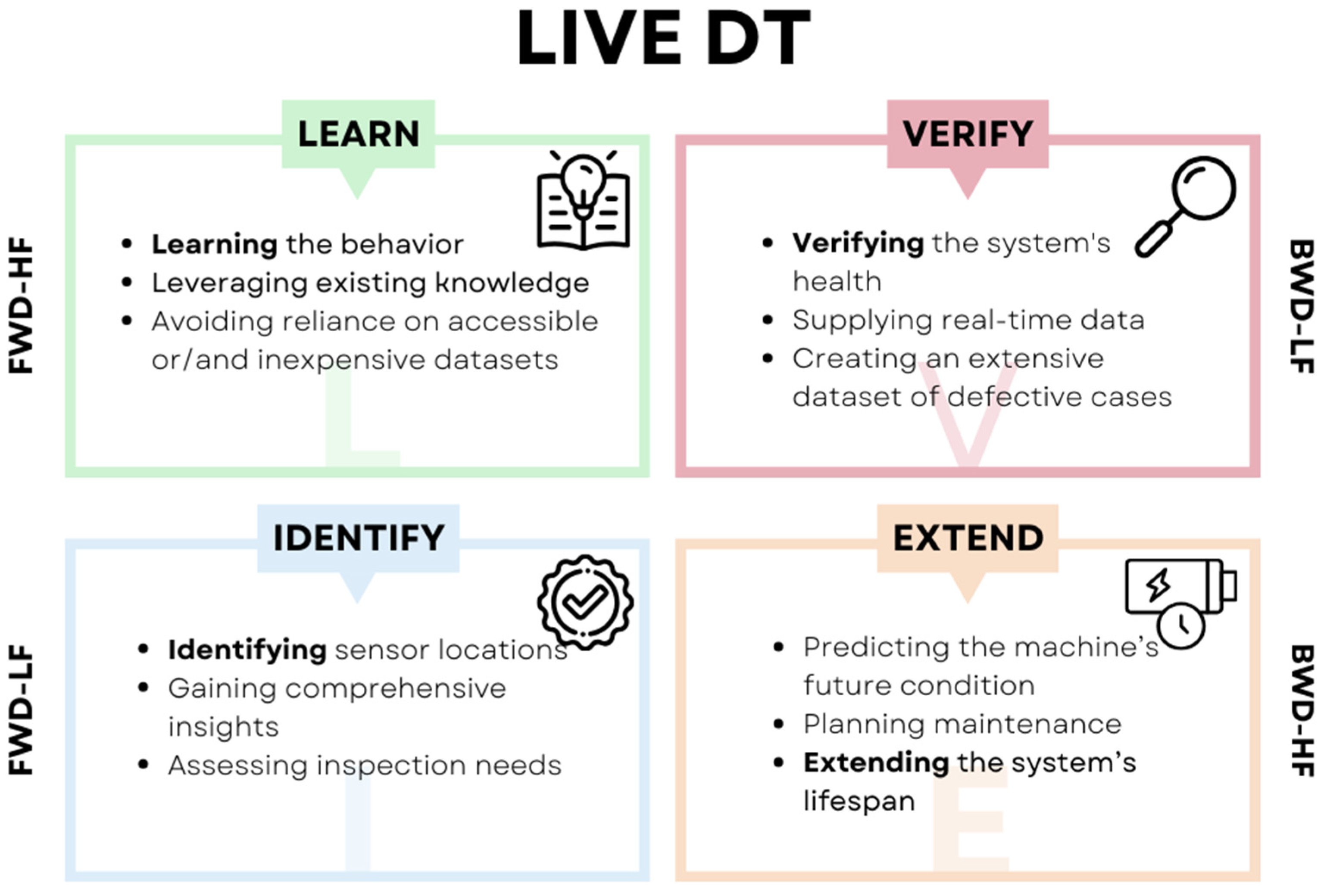
To tackle these challenges, AD2M Labs developed an innovative approach. N.G. Malek et al. [19] introduced this method, named LIVE DT, where “LIVE” represents the four primary stages: Learning, Identifying, Verifying, and Extending.

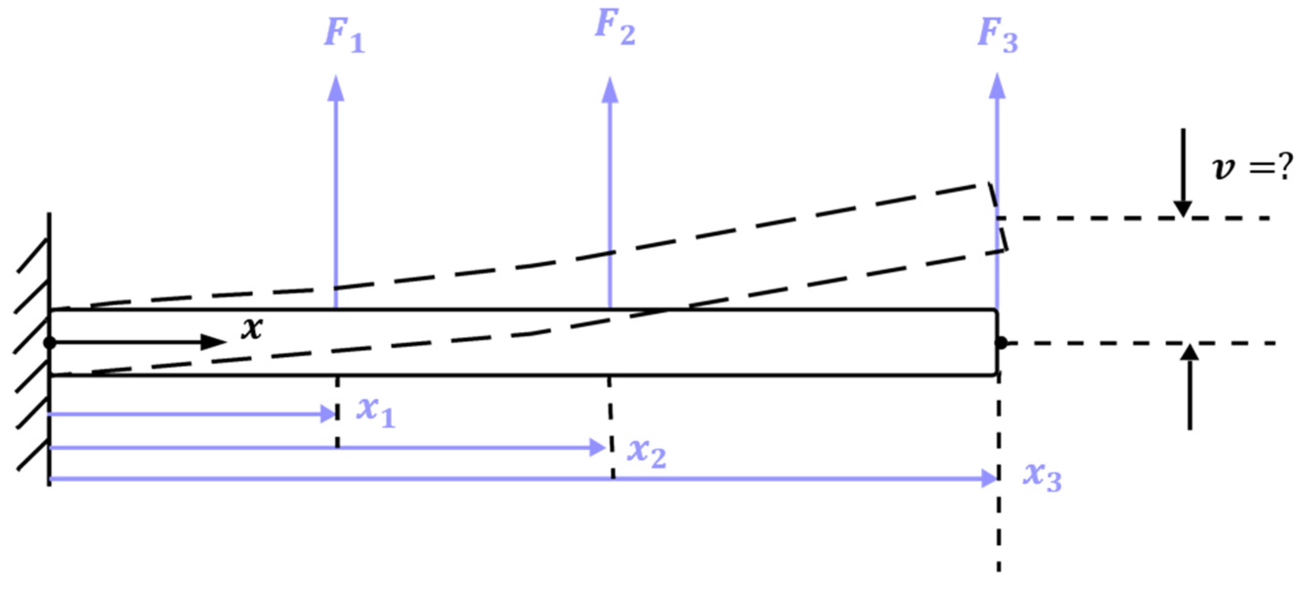
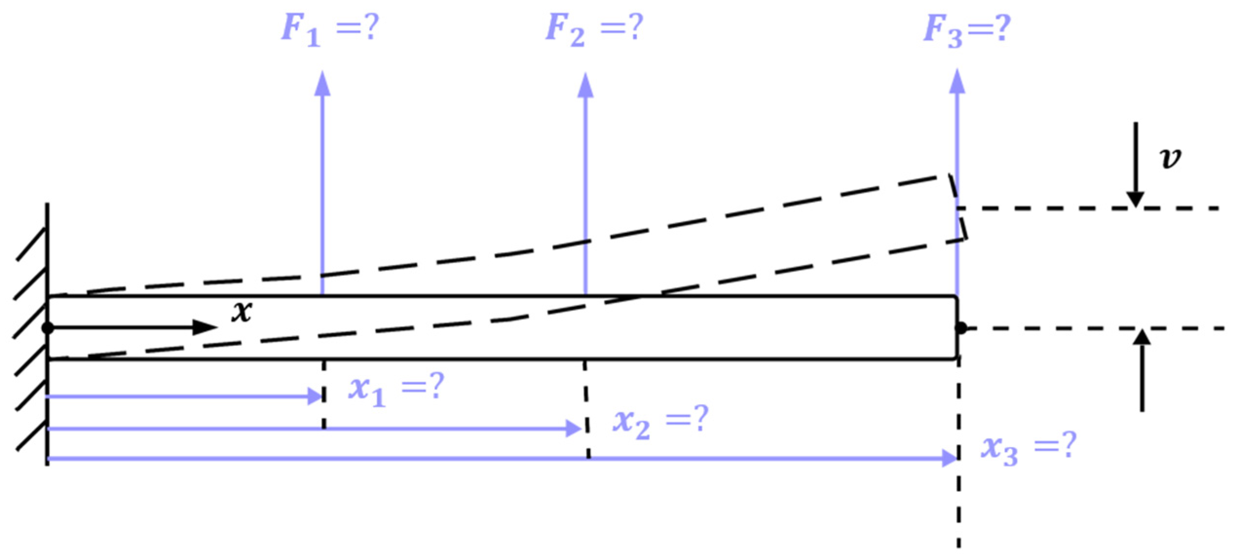
LIVE DT consists of two distinct modes: Forward (FWD) simulation and Backward (BWD) simulation. FWD simulation is typically used to determine a system’s response, often through a physics-based approach, while BWD simulation relies on a data-driven method to identify all potential external influences. Figure 1 and Figure 2 demonstrate these two different types of simulation.

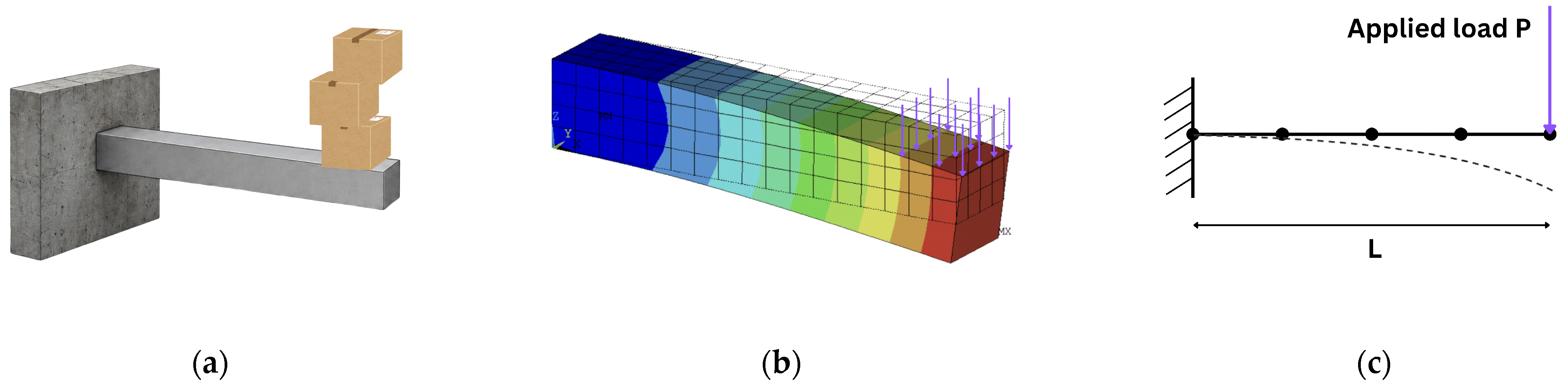
Additionally, LIVE DT employs two other types of simulations. High-Fidelity (HF) simulations provide detailed and complex analyses whereas Low-Fidelity (LF) models offer simplified representations of the physical entity (Figure 3).

The four stages of LIVE DT are shown in Figure 4. This approach has proven successful in applications such as piping systems [19] and railing systems [20]. A significant advantage of LIVE DT is its emphasis on LF simulations which allow for rapid yet fairly accurate assessments.

Low-Fidelity modelling plays a significant role in the automotive industry, particularly during the initial stages of design. At this phase, employing rapid and efficient analysis techniques is essential, as it helps streamline the process and reduces time consumption in later development stages [21]. To address this need, S. Tebby et al. [21] proposed the Simple Structural Beam (SSB) method, which is based on Finite Element Analysis. This approach simplifies intricate systems by representing them with equivalent beam structures that are carefully calibrated to ensure accuracy, aligning with experimental data from the original model. Typically, optimization techniques are applied to fine-tune the SSB model for precise results.

SSB serves as a valuable tool for the initial stages of design and the development of the LF model within the LIVE DT framework. However, its application is limited to static and modal analysis. On the other hand, existing commercial software solutions tend to be slow, inefficient, and prone to integration issues, lacking the flexibility necessary for LIVE DT. Therefore, a new LF simulation tool is required to support dynamic analysis [22].

This study aims to develop a fast and efficient LF model using beam finite elements. Given its relevance to structural dynamics, it is named Simple Structural Dynamics (SSD). Designed for high-speed performance, SSD will be compatible with weaker processors and computing units while enabling real-time data acquisition, analysis, diagnosis, and corrective actions.

The primary focus of this paper is on rotary machinery. To validate the results, SSD models will be compared with those generated by commercial Finite Element Method (FEM) software and experimental data. The data generated by SSD will be instrumental in analyzing system behavior and training machine learning algorithms.

2. Methods

This project introduces the SSD method, which utilizes basic beam elements to model rotary systems for both modal and transient dynamic simulations. Built on finite element methods and Newmark’s time integration scheme, SSD provides an efficient approach to analyzing such systems.

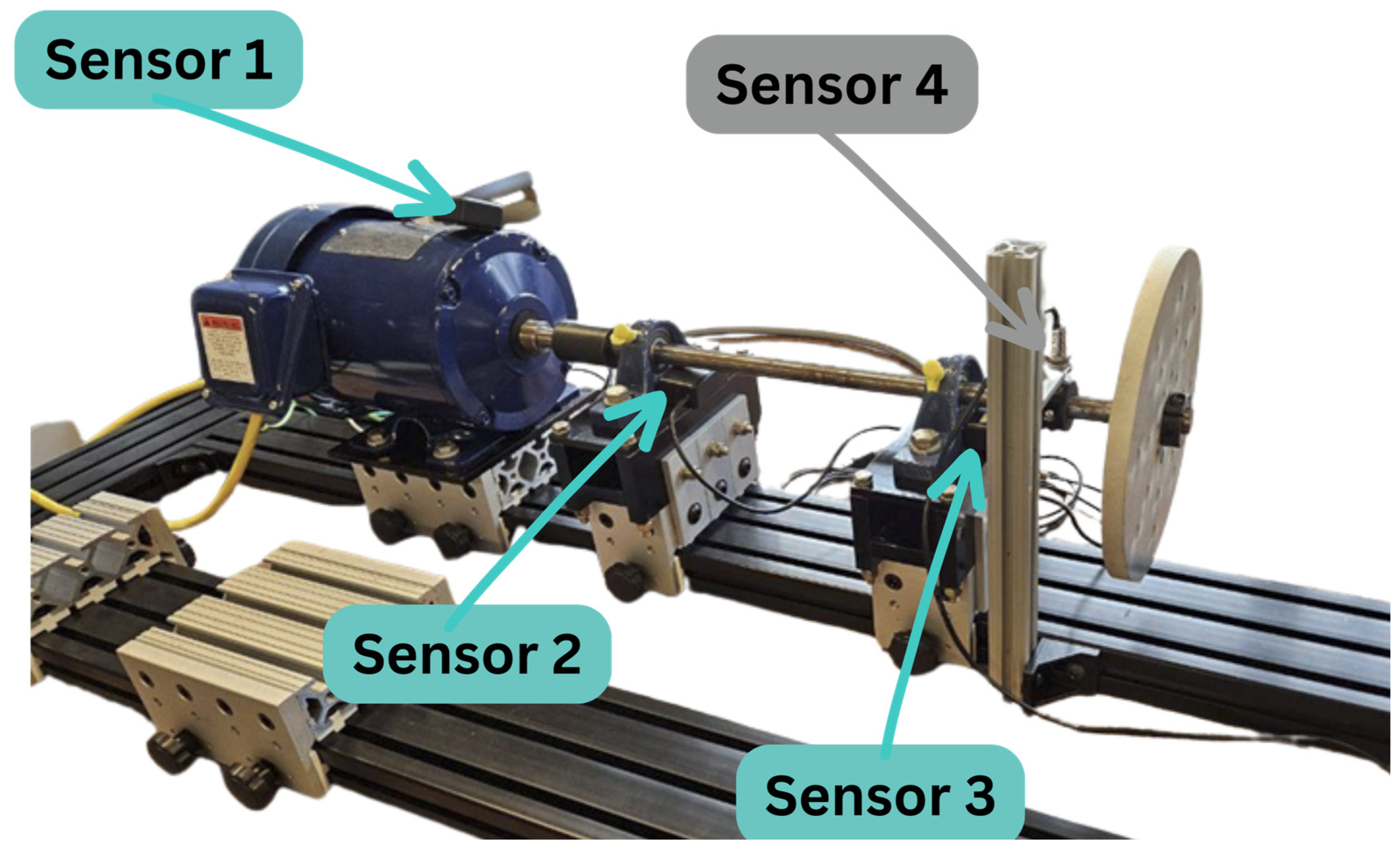
Figure 5 shows the experimental setup that was built to validate LF and HF data and investigate the accuracy and efficiency of these simulations. The setup used four sensors: three accelerometers (Sensors 1–3) and one RPM sensor (Sensor 4). The accelerometers record motor acceleration, while the RPM sensor verifies that the motor operates at the target speed.

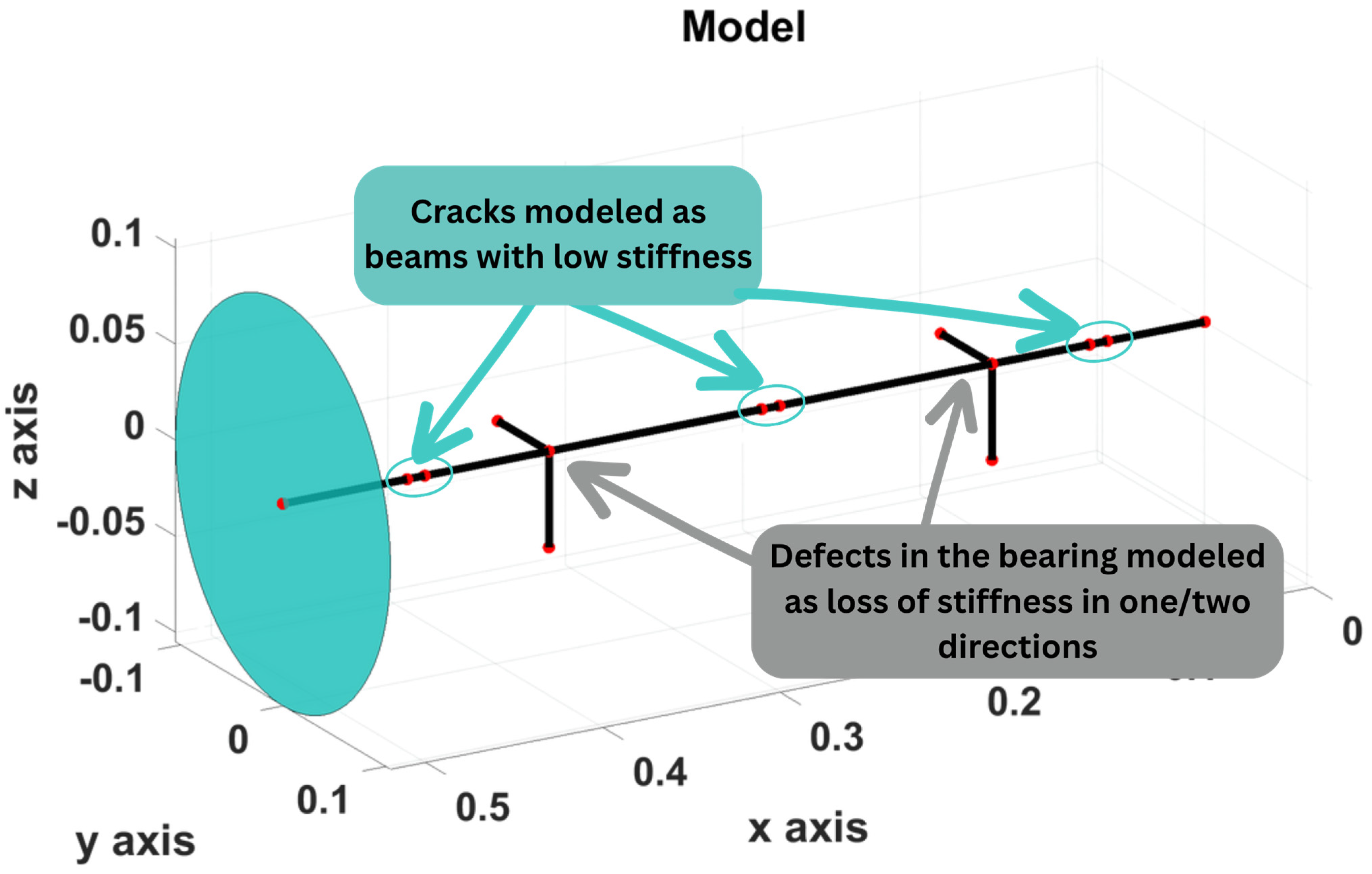
In the SSD, elements are modelled as a beam assembly. Different components in the original test setup can be simplified as beam and spring assemblies (Figure 6). For example, the bearings, shafts, and flywheel are modelled as two perpendicular springs and beam elements. In addition, the flywheel is represented by the flywheel’s weight alongside the unbalanced forces in the $y$ and $z$ directions.

Furthermore, various faulty parts can be incorporated into the SSD model. Cracks in shafts, different bearing faults (including inner and outer line defects and spalls), and unbalance in the flywheel are some of the most occurring imperfections that can affect the machine’s performance and ultimately lead to system failure.

In the SSD, cracks appearing in a shaft can be represented by small beams with reduced stiffness (Figure 6). A similar concept was applied to the faulty bearings by reducing the bearing stiffness in one or two directions [22].

2.1. Dynamic Version of Finite Element Method

FEM is applicable to both static and dynamic analyses. In the static analysis, only stiffness matrices are required. However, in the dynamic FEM, constructing mass matrices is equally essential. Additionally, after determining the mass and stiffness matrices, the dynamic equation of motion must be solved to obtain the corresponding displacements.

2.1.1. Stiffness Matrices

The LF model is composed of n nodes and p beam elements, where each node experiences six Degrees of Freedom (DOF). Each beam element has a corresponding stiffness and mass matrix, $k^e$ and $m^e$ respectively. The local stiffness matrix, $k^e$, for an element is given by the following matrix [23]:

$${[k}^e]=\left[\begin{array}{cccccccccccc}{\displaystyle \frac{A_e{E}_e}{l_e}}& 0& 0& 0& 0& 0& -{\displaystyle \frac{A_e{E}_e}{l_e}}& 0& 0& 0& 0& 0\\ 0& {\displaystyle \frac{12E_e{I}_z}{{l_e}^3}}& 0& 0& 0& {\displaystyle \frac{6E_e{I}_z}{l_e^2}}& 0& -{\displaystyle \frac{12E_e{I}_z}{l_e^3}}& 0& 0& 0& {\displaystyle \frac{6E_e{I}_z}{l_e^2}}\\ 0& 0& {\displaystyle \frac{12E_e{I}_y}{l_e^3}}& 0& -{\displaystyle \frac{6E_e{I}_y}{l_e^2}}& 0& 0& 0& -{\displaystyle \frac{12E_e{I}_y}{l_e^3}}& 0& -{\displaystyle \frac{6E_e{I}_y}{l_e^2}}& 0\\ 0& 0& 0& {\displaystyle \frac{G_e{J}_e}{l_e}}& 0& 0& 0& 0& 0& -{\displaystyle \frac{G_e{J}_e}{l_e}}& 0& 0\\ 0& 0& -{\displaystyle \frac{6E_e{I}_y}{l_e^2}}& 0& {\displaystyle \frac{4E_e{I}_z}{l_e}}& 0& 0& 0& {\displaystyle \frac{6E_e{I}_y}{l_e^2}}& 0& {\displaystyle \frac{2E_e{I}_y}{l_e}}& 0\\ 0& {\displaystyle \frac{6E_e{I}_z}{{l_e}^2}}& 0& 0& 0& {\displaystyle \frac{4E_e{I}_z}{l_e}}& 0& -{\displaystyle \frac{6E_e{I}_z}{l_e^2}}& 0& 0& 0& {\displaystyle \frac{2E_e{I}_z}{l_e}}\\ -{\displaystyle \frac{A_e{E}_e}{l_e}}& 0& 0& 0& 0& 0& {\displaystyle \frac{A_e{E}_e}{l_e}}& 0& 0& 0& 0& 0\\ 0& -{\displaystyle \frac{12E_e{I}_z}{{l_e}^3}}& 0& 0& 0& -{\displaystyle \frac{6E_e{I}_z}{l_e^2}}& 0& {\displaystyle \frac{12E_e{I}_z}{l_e^3}}& 0& 0& 0& -{\displaystyle \frac{6E_e{I}_z}{l_e^2}}\\ 0& 0& -{\displaystyle \frac{12E_e{I}_y}{l_e^3}}& 0& {\displaystyle \frac{6E_e{I}_y}{l_e^2}}& 0& 0& 0& {\displaystyle \frac{12E_e{I}_y}{l_e^3}}& 0& {\displaystyle \frac{6E_e{I}_y}{l_e^2}}& 0\\ 0& 0& 0& -{\displaystyle \frac{G_e{J}_e}{l_e}}& 0& 0& 0& 0& 0& {\displaystyle \frac{G_e{J}_e}{l_e}}& 0& 0\\ 0& 0& -{\displaystyle \frac{6E_e{I}_y}{l_e^2}}& 0& {\displaystyle \frac{2E_e{I}_y}{l_e}}& 0& 0& 0& {\displaystyle \frac{6E_e{I}_y}{l_e^2}}& 0& {\displaystyle \frac{4E_e{I}_y}{l_e}}& 0\\ 0& {\displaystyle \frac{6E_e{I}_z}{l_e^2}}& 0& 0& 0& {\displaystyle \frac{2E_e{I}_z}{l_e}}& 0& -{\displaystyle \frac{6E_e{I}_z}{l_e^2}}& 0& 0& 0& {\displaystyle \frac{4E_e{I}_z}{l_e}}\end{array}\right]$$

(1)

where $A_e$ is the cross-sectional area, $I_y$ and $I_z$ are the moments of inertia about the $y$ and $z$ axis, $J_e$ is the polar moment of inertia, $E_e$ is Young’s Modulus, $G_e$ is the Shear Modulus, and $l_e$ is the length of the beam element.

2.1.2. Mass Matrices

This section outlines the step-by-step procedure for conducting dynamic analysis using FEM. The initial step involves choosing the appropriate type of element, with beam elements being used in SSD simulations. The second step is selecting the displacement function, typically expressed in terms of shape functions ($N$). The strain ($\epsilon$)–nodal displacement ($q$) and stress ($\sigma$)–displacement relationships must be defined. The $\epsilon -q$ relationship can be expressed as [23]:

$$\left\{\epsilon \right\}=\left[B\right]\left\{q\right\}$$

(2)

where $\left[B\right]$ is the element strain—displacement matrix.

In this case, as the element is assumed to be of the beam type, Hooke’s law [24] applies. The third step in the process involves expressing stress in the following matrix form

$$\left\{\sigma \right\}=\left[D\right]\left\{\epsilon \right\}=\left[D\right]\left[B\right]\left\{q\right\}$$

(3)

where $\left[D\right]$ in this case is equal to $E$ based on the Hooke’s law.

The process of deriving the element stiffness and mass matrices constitutes the fourth step. When it comes to expressing the mass matrices, two methods are available. The first and simplest method assumes that the masses are equally distributed and lumped at the two ends of the bar. As a result, the mass matrix obtained through this approach is referred to as the lumped-mass matrix.

The lumped-mass method has certain advantages, such as the simplicity of the lumped-mass matrix, which makes it more convenient for manual calculations. Despite this, its accuracy is relatively low. To overcome this drawback, consistent-mass matrices were introduced as a more precise alternative, eventually replacing lumped-mass matrices.

Consistent-mass matrices are generally derived using the virtual work principle [24]. Nevertheless, it is more convenient to use D’ Alembert’s principle [24]. To use, D’ Alembert’s approach effective body forces are defined using Newton’s second law according to the assumption that acceleration creates forces on the opposite direction of acceleration. The effective body forces, therefore, can be written as

$${\{X}^e\}=-\rho \{\ddot{u}\}$$

(4)

where ${\{X}^e\}$ is the vector of body forces and $\left\{\ddot{u}\right\}$ is the acceleration vector. The negative sign in the equation above is since the produced forces are in the opposite direction of the acceleration.

Nodal body forces of the element can be derived as follows using the energy method [24]:

$$\left\{f_b\right\}={\iiint }_V{\left[N\right]}^T{\{X}^e\}dV$$

(5)

Substituting the acceleration from equation and using $\left\{\ddot{u}\right\}=\left[N\right]\left\{\ddot{d}\right\}$:

$$\left\{f_b\right\}=-{\iiint }_V{\left[N\right]}^T\ddot{u}dV=-{\iiint }_V{\left[N\right]}^T\left[N\right]\ddot{q}dV=-\left[m_e\right]\left\{\ddot{q}\right\}$$

(6)

$\left[m^e\right]$ in the equation above is the consistent mass matrix as:

$$\left[m^e\right]=-{\iiint }_V\rho {\left[N\right]}^T\left[N\right]dV$$

(7)

As an example, using this method and transforming the resulting matrix the following consistent-mass matrix for a 6-DOF frame element can be obtained [23]:

$${[m}^e]={\rho }_e{A}_e{l}_e\left[\begin{array}{cccccccccccc}{\displaystyle \frac{1}{3}}& 0& 0& 0& 0& 0& {\displaystyle \frac{1}{6}}& 0& 0& 0& 0& 0\\ 0& {\displaystyle \frac{13}{35}}& 0& 0& 0& {\displaystyle \frac{11l_e}{210}}& 0& {\displaystyle \frac{9}{70}}& 0& 0& 0& -{\displaystyle \frac{13l_e}{420}}\\ 0& 0& {\displaystyle \frac{13}{35}}& 0& -{\displaystyle \frac{11l_e}{210}}& 0& 0& 0& {\displaystyle \frac{9}{70}}& 0& {\displaystyle \frac{13l_e}{420}}& 0\\ 0& 0& 0& {\displaystyle \frac{I_y+I_z}{3A_e}}& 0& 0& 0& 0& 0& {\displaystyle \frac{I_y+I_z}{6A_e}}& 0& 0\\ 0& 0& -{\displaystyle \frac{11l_e}{210}}& 0& {\displaystyle \frac{{l_e}^2}{105}}& 0& 0& 0& -{\displaystyle \frac{13l_e}{420}}& 0& {\displaystyle \frac{-{l_e}^2}{140}}& 0\\ 0& {\displaystyle \frac{11l_e}{210}}& 0& 0& 0& {\displaystyle \frac{{l_e}^2}{105}}& 0& {\displaystyle \frac{13l_e}{420}}& 0& 0& 0& -{\displaystyle \frac{{l_e}^2}{140}}\\ {\displaystyle \frac{1}{6}}& 0& 0& 0& 0& 0& {\displaystyle \frac{1}{3}}& 0& 0& 0& 0& 0\\ 0& {\displaystyle \frac{9}{70}}& 0& 0& 0& {\displaystyle \frac{13l_e}{420}}& 0& {\displaystyle \frac{13}{35}}& 0& 0& 0& -{\displaystyle \frac{11l_e}{210}}\\ 0& 0& {\displaystyle \frac{9}{70}}& 0& -{\displaystyle \frac{13l_e}{420}}& 0& 0& 0& {\displaystyle \frac{13}{35}}& 0& {\displaystyle \frac{11l_e}{210}}& 0\\ 0& 0& 0& {\displaystyle \frac{I_y+I_z}{6A_e}}& 0& 0& 0& 0& 0& {\displaystyle \frac{I_y+I_z}{3A_e}}& 0& 0\\ 0& 0& {\displaystyle \frac{13l_e}{420}}& 0& {\displaystyle \frac{-{l_e}^2}{140}}& 0& 0& 0& {\displaystyle \frac{11l_e}{210}}& 0& {\displaystyle \frac{{l_e}^2}{105}}& 0\\ 0& -{\displaystyle \frac{13l_e}{420}}& 0& 0& 0& {\displaystyle \frac{-{l_e}^2}{140}}& 0& -{\displaystyle \frac{11l_e}{210}}& 0& 0& 0& {\displaystyle \frac{{l_e}^2}{105}}\end{array}\right]$$

(8)

where $\rho$ is density of the beam element.

Global stiffness, $\left[K\right]$, and global mass, $\left[M\right]$, matrices can be constructed using the following equations:

$$[K]= {\displaystyle \sum _{i=1}^p}\left[k_i^e\right]$$

(9)

$$[M]={\displaystyle \sum _{i=1}^p}{[m}_i^e]$$

(10)

where the global stiffness and mass matrix, $\left[K\right]$ and $\left[M\right]$, are the summation of the local matrices $\left[k_i^e\right]$ and ${[m}_i^e]$ and, $p$ is the total number of elements in the LF model.

And the general form of the motion equation is

$$\left\{f\left(t\right)\right\}=\left[K\right]\left\{q\right\}+\left[M\right]\left\{\ddot{q}\right\}$$

(11)

2.1.3. Rigid Body Motion

When using the Finite Element Method to model a dynamic problem, one potential challenge is the rigid body motion. This occurs because rigid body motion causes the system’s stiffness matrix to become singular, making it impossible to solve the equations of motion using standard methods. A common example is a rotating shaft that maintains a constant speed without experiencing substantial resistance in its rotational direction.

To address this issue, it is necessary to impose appropriate boundary conditions, also known as constraints. The number of required boundary conditions corresponds to the number of rigid body modes present in the system. These constraints, referred to as nonhomogeneous boundary conditions, involve prescribed displacements.

The solution process for handling rigid body motion involves the following steps:

Step (1)—Applying a prescribed displacement: For instance, in the case of a shaft rotating at a constant speed, an incremental rotational displacement can be introduced as a nonhomogeneous boundary condition.

Step (2)—Matrix partitioning: In this step, Equation (11) must be partitioned accordingly to facilitate the solution

$$\left[\begin{array}{cc}{[m}_{11}]& {[m}_{12}]\\ {[m}_{21}]& {[m}_{22}]\end{array}\right]\left\{\begin{array}{c}{\displaystyle \frac{{\mathsf{\partial }}^2{\overrightarrow{Q}}_1}{\mathsf{\partial }{t}^2}}\\ {\displaystyle \frac{{\mathsf{\partial }}^2{\overrightarrow{Q}}_2}{\mathsf{\partial }{t}^2}}\end{array}\right\}+\left[\begin{array}{cc}{[k}_{11}]& {[k}_{12}]\\ {[k}_{21}]& {[k}_{22}]\end{array}\right]\left\{\begin{array}{c}{\overrightarrow{Q}}_1\\ {\overrightarrow{Q}}_2\end{array}\right\}=\left\{\begin{array}{c}{\overrightarrow{F}}_1\\ {\overrightarrow{F}}_2\end{array}\right\}$$

(12)

where

$$\left\{f\left(t\right)\right\}=\left\{\begin{array}{c}{\overrightarrow{F}}_1\\ {\overrightarrow{F}}_2\end{array}\right\}$$

(13)

$$\left[K\right]=\left[\begin{array}{cc}{[k}_{11}]& {[k}_{12}]\\ {[k}_{21}]& {[k}_{22}]\end{array}\right]$$

(14)

$$\left[M\right]=\left[\begin{array}{cc}{[m}_{11}]& {[m}_{12}]\\ {[m}_{21}]& {[m}_{22}]\end{array}\right]$$

(15)

and ${\overrightarrow{Q}}_1$ is the vector of unconstrained displacements while ${\overrightarrow{Q}}_2$ is the vector of constrained displacements.

Step (3)—Once the vector partitioning is complete, the next step is to derive the active stiffness matrix, mass matrix, and force vectors. This process is governed by Equation (12):

$${[m}_{11}]{\overrightarrow{\ddot{Q}}}_1+{[k}_{11}]{\overrightarrow{Q}}_1={\overrightarrow{F}}_1-\left[k_{12}\right]{\overrightarrow{Q}}_2-[m_{12}]{\overrightarrow{\ddot{Q}}}_2$$

(16)

In our applications, we primarily analyze the system’s behavior in a steady-state condition, where the rotational speed remains constant. Under this assumption, the ${\overrightarrow{\ddot{Q}}}_2$ term on the right-hand side of the equation can be neglected. As a result, the active matrices and force vectors are defined as:

$$\left[k_{act}\right]={[k}_{11}]$$

(17)

$$\left[m_{act}\right]={[m}_{11}]$$

(18)

$${\overrightarrow{F}}_{act}={\overrightarrow{F}}_1-\left[k_{12}\right]{\overrightarrow{Q}}_2$$

(19)

Here, $\left[k_{act}\right]$, $\left[m_{act}\right]$, and ${\overrightarrow{F}}_{act}$ represent the active stiffness matrix, mass matrix, and force vector, respectively.

2.2. Frequency-Dependent Dynamic Analysis

Once the local stiffness and mass matrices are obtained for different element types, they must be assembled to construct the global stiffness and mass matrices. Before conducting a time-dependent analysis, it is essential to first perform a modal analysis (i.e., a frequency-dependent dynamic analysis). This step is crucial because both free and forced vibration responses can be expressed as a superposition of modes [25]. Modal analysis is widely applied in various applications, including early-stage design in the early design phases [26], FEA calibration [27], and sensor optimization [28].

For an undamped system subject to external loading, the governing equation of motion is presented in Equation (11). However, under the assumption of undamped free vibration, this equation becomes:

$$\left[K\right]\left\{q\right\}+\left[M\right]\left\{\ddot{q}\right\}=0$$

(20)

The structure can be analyzed under the conditions of a modal analysis and extract various vibrational characteristics. To achieve this, Equation (21) can be rearranged as:

$$\left|\left[K\right]- {\omega }^2\left[M\right]\right|=0$$

(21)

where the beam-model’s natural frequencies of vibration, $\omega$, can be calculated using global stiffness. Applying the following equation to the structure will extract the pairing mode shapes:

$$\left|\left[K\right]- {\omega }_m^2\left[M\right]\right|{\phi }_m=0$$

(22)

This is a classical eigen-value problem with many previous methods used to solve the eigen-values and eigen-vectors. Where $\omega$ are the natural frequencies (eigen-values) and $\phi$ are the mode shapes (eigen-vectors). In Equation (22) the mth natural frequency, ${\omega }_m$, has a corresponding mode shape, ${\phi }_m$.

The calculated eigenvalues correspond to the system’s natural frequencies, while the associated eigenvectors represent the mode shapes. Among the computed natural frequencies, the fundamental natural frequency holds the greatest significance [29].

2.3. Time-Dependent Dynamic Analysis

Numerical integration in the time domain is essential for performing time-dependent dynamic simulations. The most widely used approach for this purpose is the use of direct integration methods, of which several variations exist in the literature. One example is the central difference method, which follows an explicit integration approach [30]. The central difference method is quite simple to apply and is one of the earliest methods used for direct integration [24]. Nonetheless, implicit integration techniques are more common today. Implicit integration methods have become more prevalent due to their stability and accuracy. Different implicit techniques are available, including Newmark’s method [31], Wilson’s method [32], and Houbolt’s method [33]. Among these, Newmark’s method is one of the most widely used approaches. Therefore, Newmark’s method is utilized in this paper for time integration.

Newmark’s Method

Newmark’s equation for displacement and velocity can be derived as [31]:

$${\dot{d}}_{i+1}={\dot{d}}_i+\left[\left(1-\gamma \right){\ddot{d}}_i+{\gamma \ddot{d}}_{i+1}\right]∆t$$

(23)

$$d_{i+1}=d_i+{\dot{d}}_i∆t+\left[\left({\displaystyle \frac{1}{2}}-\beta \right){\ddot{d}}_i+{\beta \ddot{d}}_{i+1}\right]$$

(24)

In the equations above, $d_i$ represents the displacement vector at the $i$th step. $\gamma$ and $\beta$ are parameters that need to be defined by the user. Typically, $\gamma$ is ${\displaystyle \frac{1}{2}}$ and $\beta$ should have a value between 0 and ${\displaystyle \frac{1}{4}}$ [24]. Notably, the central difference method is a special case of Newmark’s method, where $\beta =0$.

3. Results and Discussion

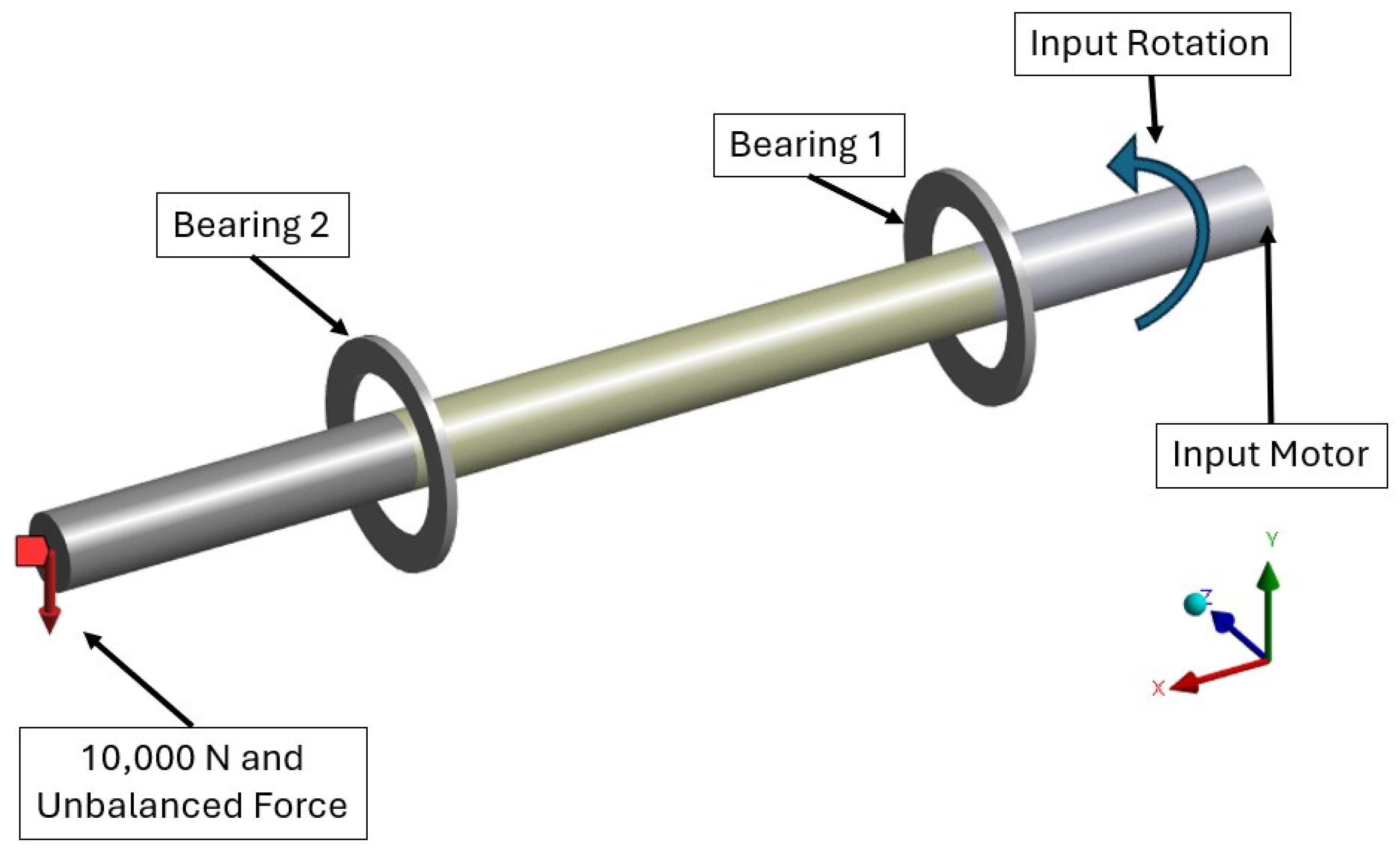
The LF results were derived and confirmed through both modal and transient analyses. This study focused on a rotary machine composed of two bearings, a shaft connected to a motor on one end, and a flywheel on the opposite end. The system was modelled as a shaft anchored at the motor end, while an unbalanced mass was applied to the flywheel, generating unbalanced forces. This setup is illustrated in Figure 7.

An HF model of the setup, without any defects (i.e., healthy system), was subjected to a 10,000 N linearly increasing force, and an unbalanced force was applied to the shaft tip. First, modal analysis was performed to acquire the natural frequencies, mode shapes, and the frequency-dependent behavior of the system.

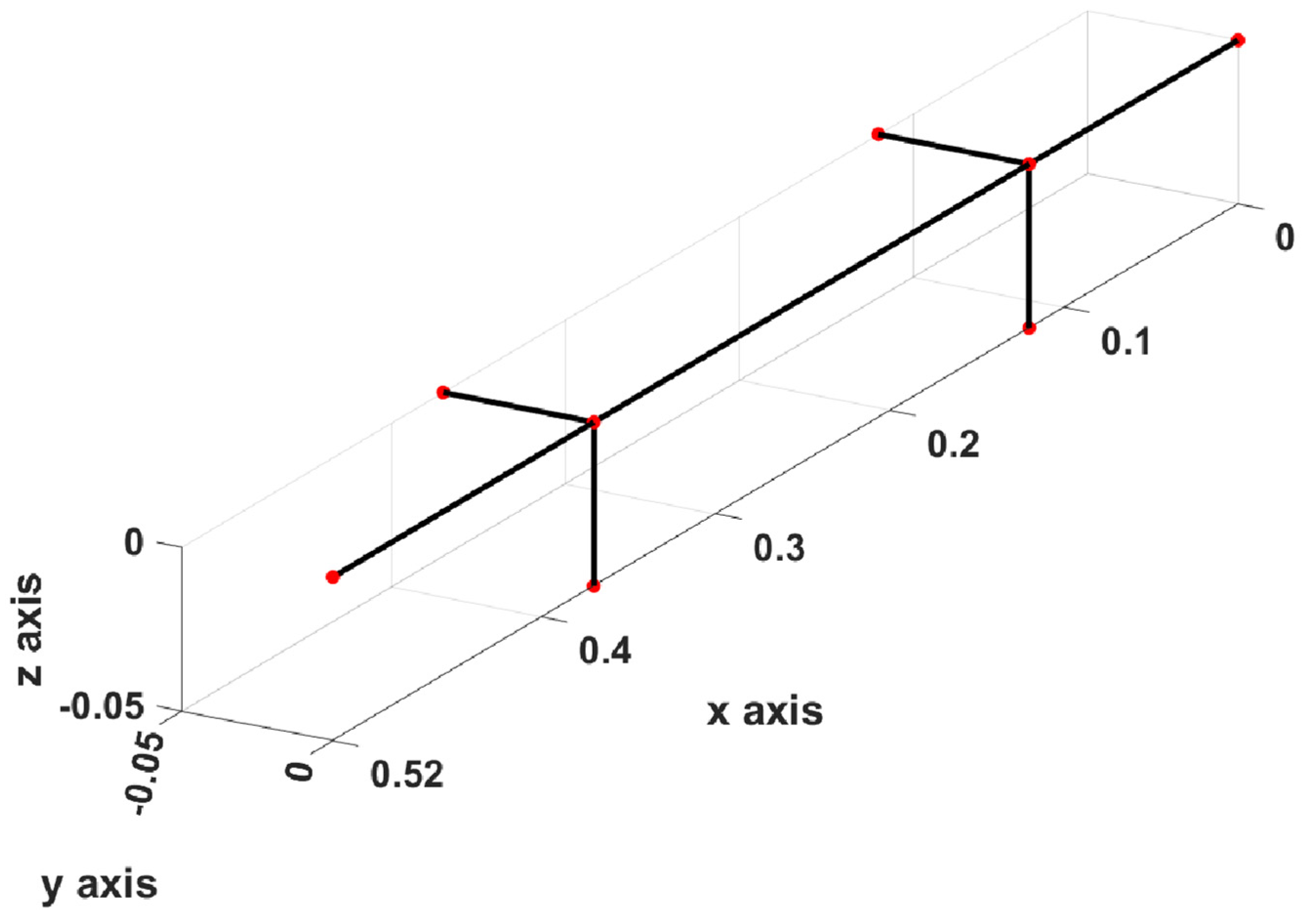
The SSD version of the system is shown in Figure 8. The shafts are modelled as simple beam elements, and the bearings are replaced by two spring elements with equivalent stiffness.

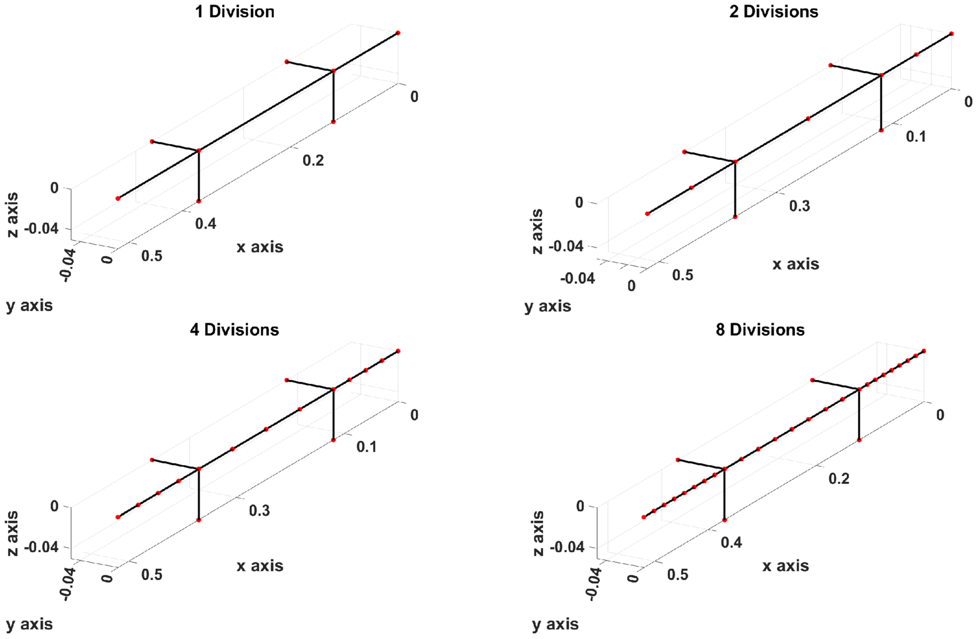
Simulations were conducted using both HF and LF methods. A commercial FEA software package was used for HF analysis. The first ten natural frequencies of the system are presented in

Table 1. Natural frequencies of the healthy system.

Mode Number	SSD (Hz)	FEA Software (Hz)	Difference (%)
1	87	87	0.0
2	87	87	0.0
3	528	512	3.0
4	528	512	3.0
5	1479	1405	5.0
6	1479	1405	5.0
7	1527	1505	1.5
8	2463	2427	1.5
9	3544	2679	24.4
10	3544	2679	24.4

. The second column shows the natural frequencies corresponding to the SSD simulation, whereas the third column contains the values obtained using commercial software. Calculated frequencies are relatively close except for the last two modes. However, this discrepancy can be reduced by increasing the number of elements in the LF model. Figure 9 illustrates how the node interpolation technique was utilized to improve the results.

The primary source of discrepancy is the difference in model fidelity between the SSD and the commercial finite element model. SSD represents the rotary system using simplified one-dimensional beam and spring elements, whereas the high-fidelity model uses detailed three-dimensional solid elements and a more complete representation of the geometry, mass distribution, stiffness distribution, and component interactions. These modelling simplifications introduce a model-form error that becomes more pronounced for higher vibration modes.

Table 2. The 10th natural frequency of the system for different numbers of divisions.

Number of Divisions	SSD (Hz)	Difference (%)
1	3544	24.4
2	2870	6.7
3	2859	6.3
4	2854	6.1
5	2852	6.1
6	2852	6.1
7	2852	6.1
8	2851	6.1
9	2851	6.1
10	2851	6.1

shows that the difference between LF and HF simulations can be reduced to 6.1% by increasing the number of divisions. This can be further reduced by calibrating the SSD model. Also, it can be observed that the results converge when at least seven nodes are inserted between the original nodes.

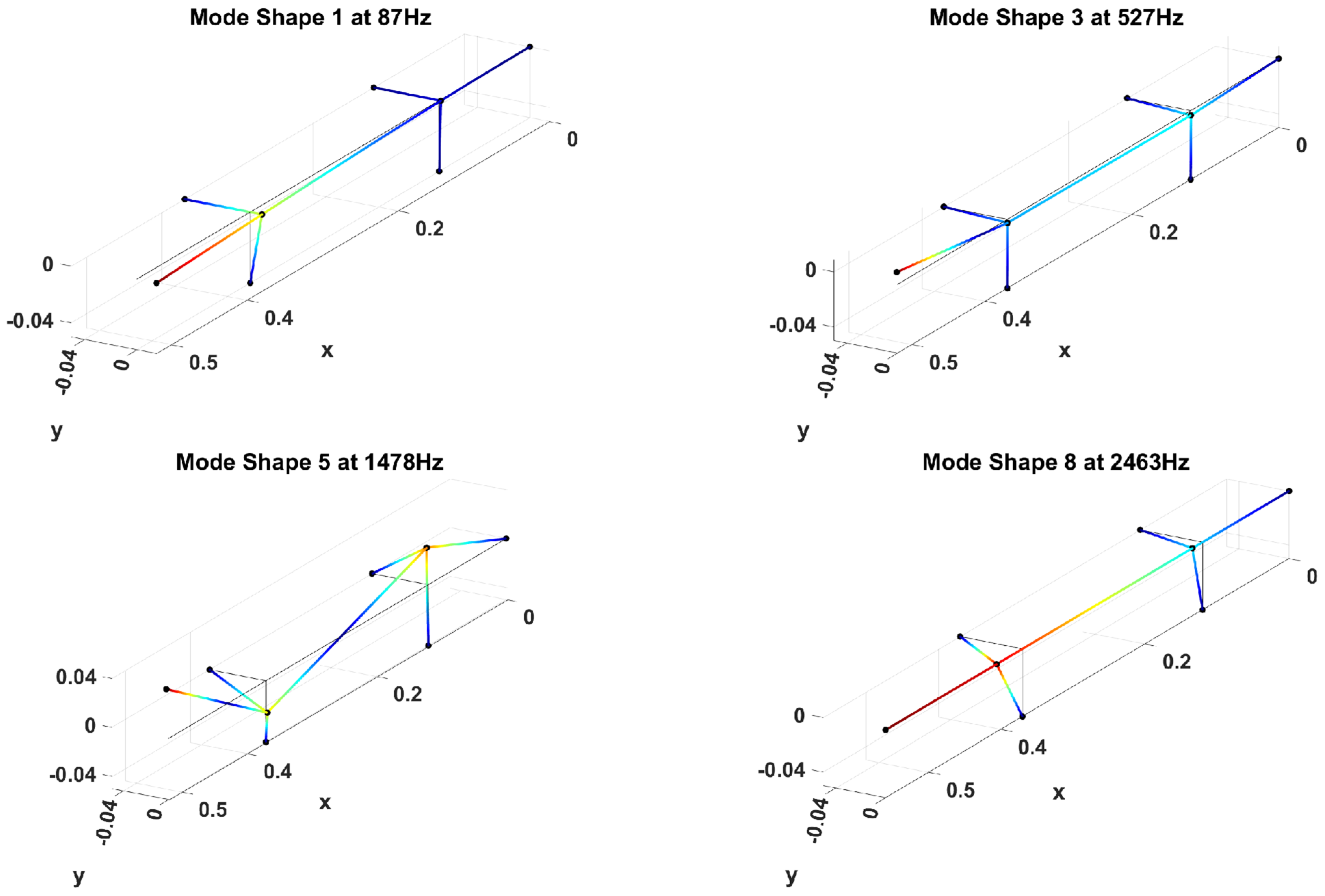
SSD can also offer insights into various mode shapes, some of which are shown in Figure 10. This means that SSD not only delivers results comparable to those of commercial FEM programs but also enhances our understanding of the system’s behavior through visualization.

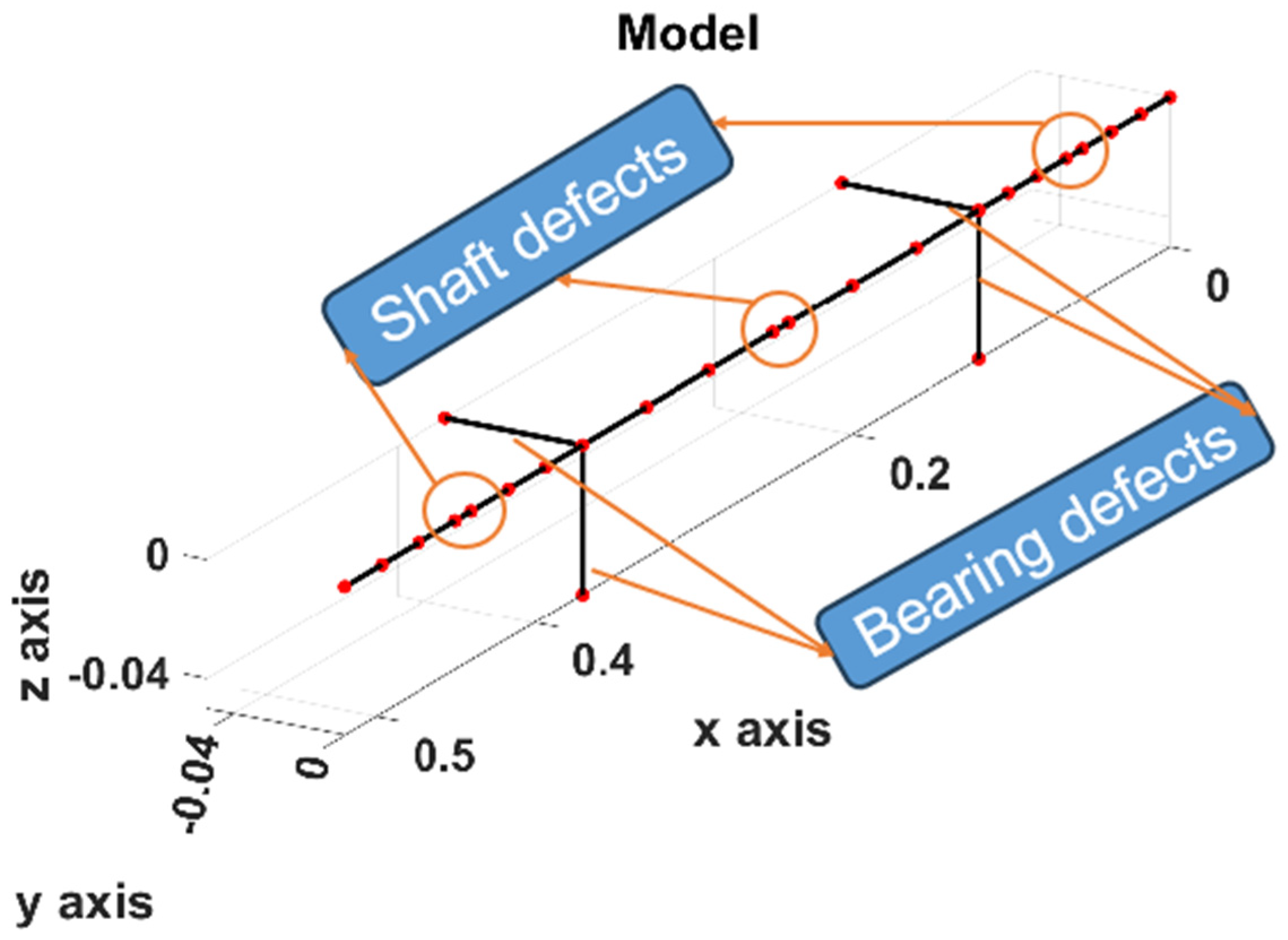
With further adjustment, the SSD model can be utilized for defective systems. These modifications are illustrated in Figure 11. Any faults in the shaft are introduced into the model using small beam element with reduced stiffness. Furthermore, the bearing elements with lowered stiffness were implemented to emulate defective bearings.

After implementing the necessary adjustments, the natural frequencies of the faulty system can be determined. These results are presented in

Table 3. A comparison between natural frequencies of healthy and defective systems.

Mode Number	SSD (Hz)-Unhealthy	SSD (Hz)-Healthy
1	79	87
2	80	87
3	493	520
4	493	520
5	1432	1455
6	1432	1455
7	1505	1505
8	2295	2427
9	2680	2851
10	2680	2851

. As anticipated, the natural frequencies of the healthy system are consistently higher due to the reduction in component stiffness. Variations in the system’s natural frequencies can serve as indicators for detecting faults in the rotary system. Furthermore, the magnitude of these changes may provide insight into the severity of the defects.

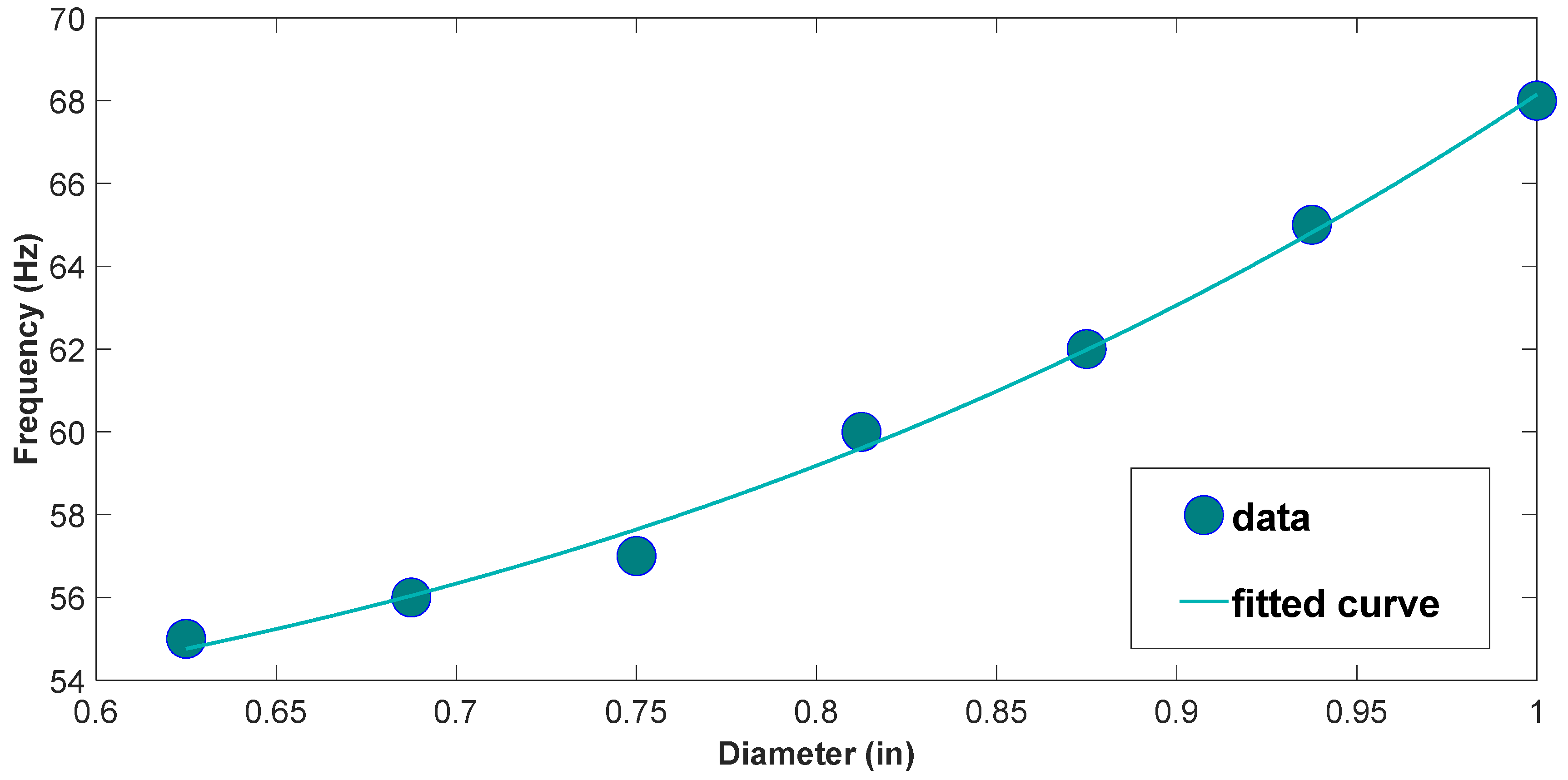
Adjustments to the input parameters can be made to analyze their effects on the system. One significant factor influencing natural frequencies is the shaft diameter. Figure 12 demonstrates how variations in shaft diameter affect the fundamental frequency of the system. The data corresponds to a defective system with a health value of 0.50, meaning that the faulty element retains only 50% of its original stiffness. The results indicate that an increase in shaft diameter leads to an increase in natural frequency. This occurs because, at larger shaft diameters, the system becomes stiffer. Since frequency is proportional to the stiffness of the system, this naturally leads to higher frequencies.

As shown so far, modal analysis can provide some insight into the state of the rotary machines. Nevertheless, it does not provide us with the whole picture. The transient analysis can be implemented as an alternative to the modal analysis. While transient analysis is more computationally expensive compared to modal analysis, it is more comprehensive. The SSD is an integrated package that can perform both modal and time-dependent simulations.

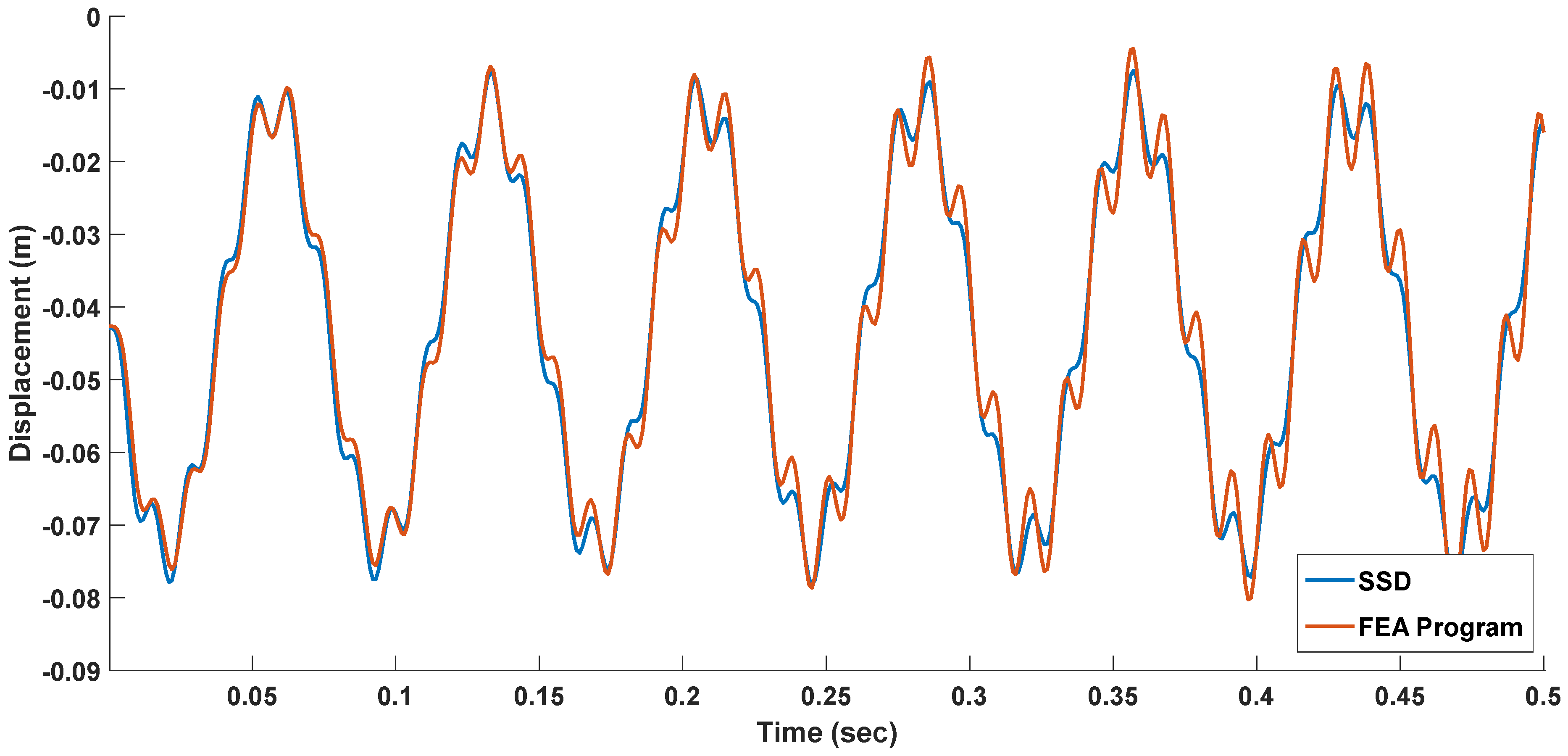
The transient analysis of the system was conducted to produce time-dependent results. The results were compared for both SSD and the commercial software package. The comparison between the transient output of both approaches is shown in Figure 13. This figure illustrates the Y-displacement of the tip of the shaft over time. It can be observed that the produced outputs are very close. However, a statistical analysis is required to confirm this observation.

Mean, variance, and kurtosis are the prevalent parameters used to compare the time-dependent data. In both methods, the mean and variance values differ by only about 1%, indicating that the datasets exhibit similar overall behavior. However, kurtosis analysis provides deeper insights into the key differences between the two output sets.

To better understand these variations, the kurtosis values for both methods were obtained. Like variance, kurtosis places greater emphasis on larger deviations while assigning less importance to smaller ones. For a normally distributed dataset, the expected kurtosis is 3 [34], but in this study, values around 1.5 were observed. Additionally, the displacement results obtained from the commercial software package were only 5.07% higher than those from SSD, further reinforcing the strong agreement between the two datasets.

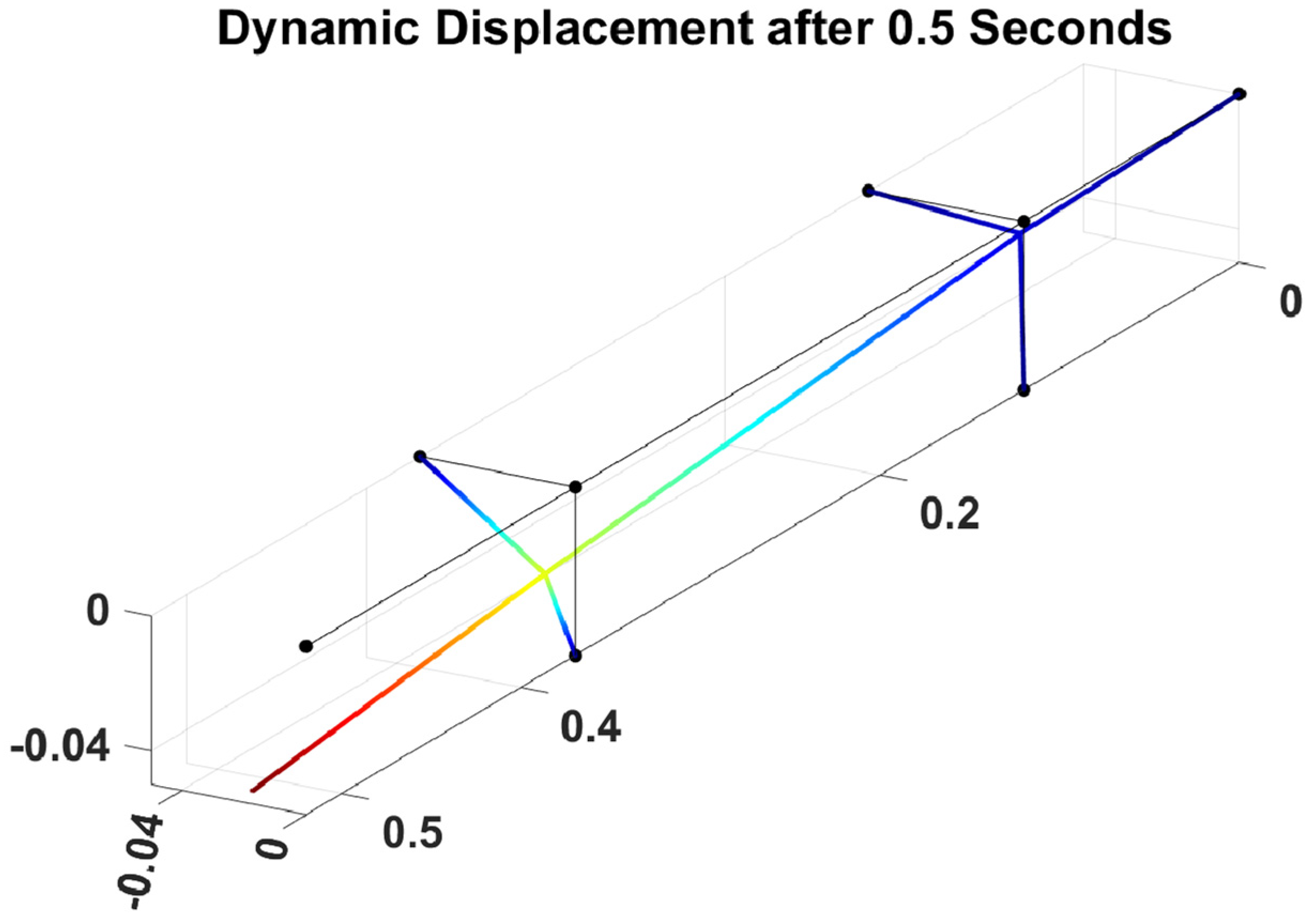
SSD also produces visual outputs that offer further insights. For instance, Figure 14. illustrates the shaft’s displacement under the influence of an unbalanced force and a constant motor rotational speed. These displacements were obtained after 0.5 s.

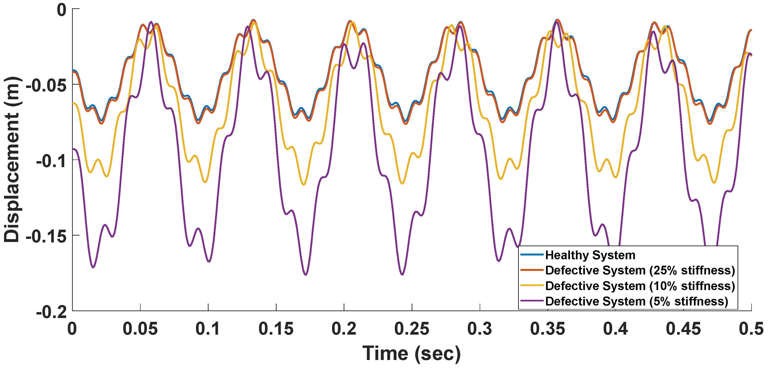
Like modal analysis, the transient analysis can also be used to model defective systems. For example, Figure 15 illustrates the impact of stiffness loss caused by defects in various system components. The results indicate that reducing the stiffness of defective parts to around 25% has minimal effect on transient outputs. However, a further decrease in stiffness leads to significant changes in the displacement response. Systems with more severe defects (i.e., greater stiffness reduction) are expected to exhibit higher amplitude responses.

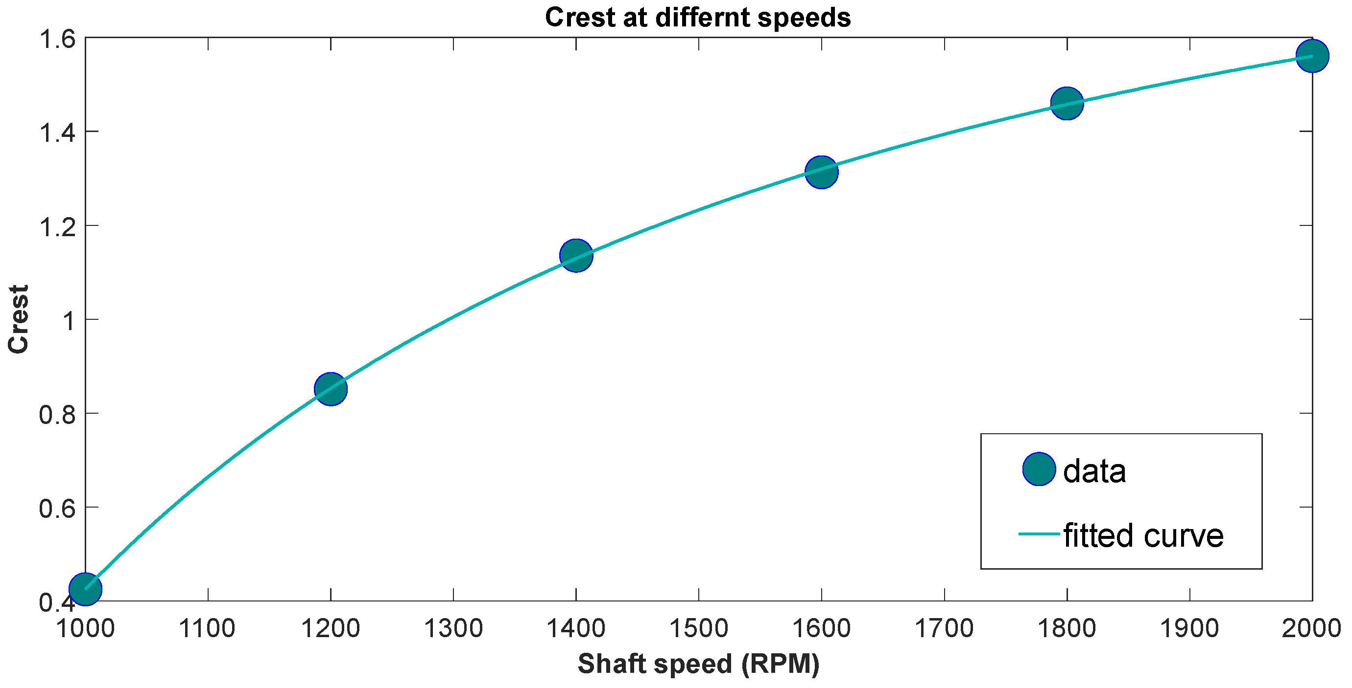
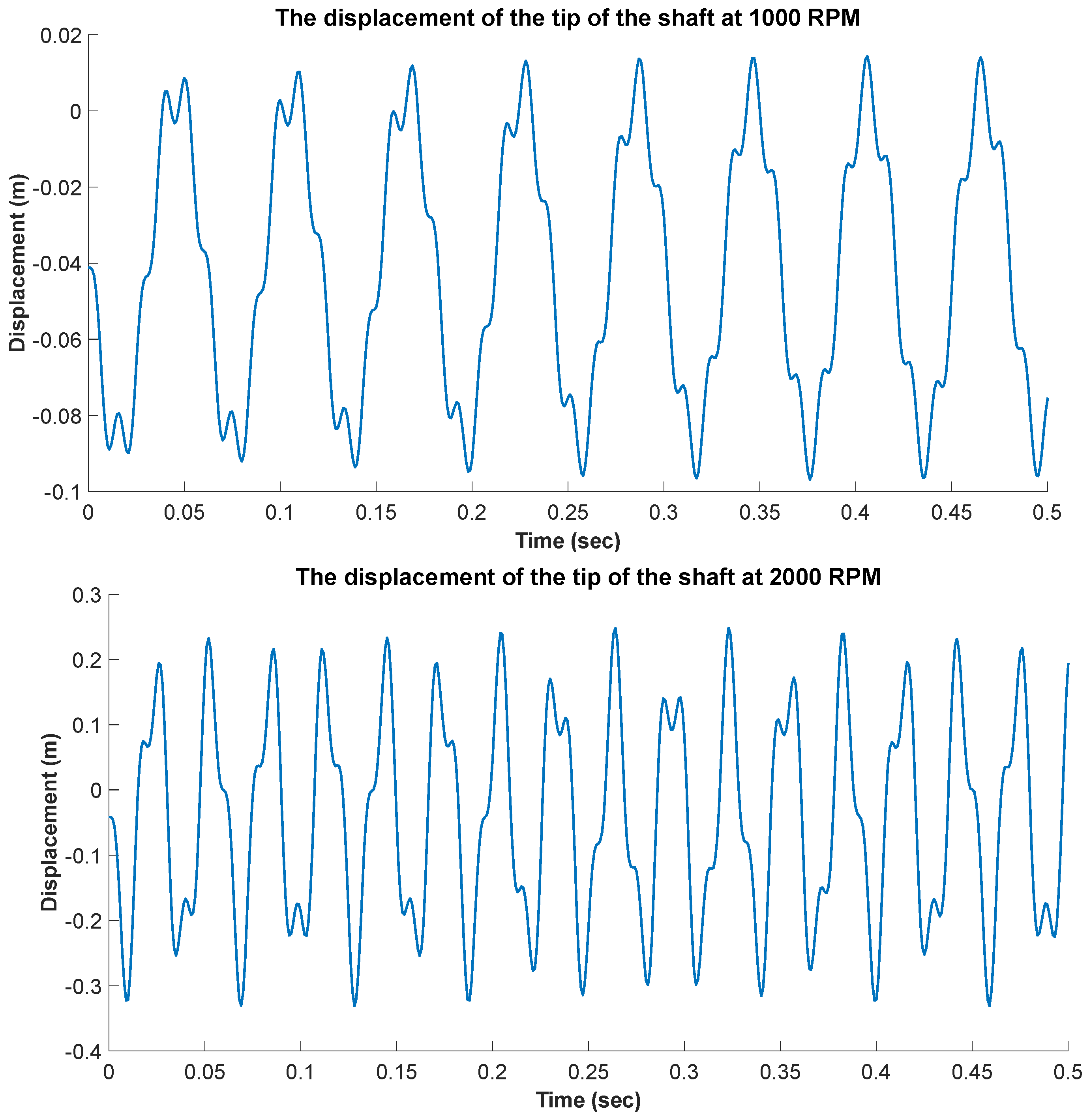
Multiple analyses were conducted to examine how certain key parameters influence the results of the transient simulations. One of these parameters is the shaft speed. As illustrated in Figure 16, the system’s dynamic response varies with changes in speed. An increase in shaft speed results in a greater number of peaks and oscillations. A similar trend is evident in Figure 17, where the crest of the data rises as the speed of the shaft increases. This outcome was anticipated, as the crest serves as an indicator of signal peakiness.

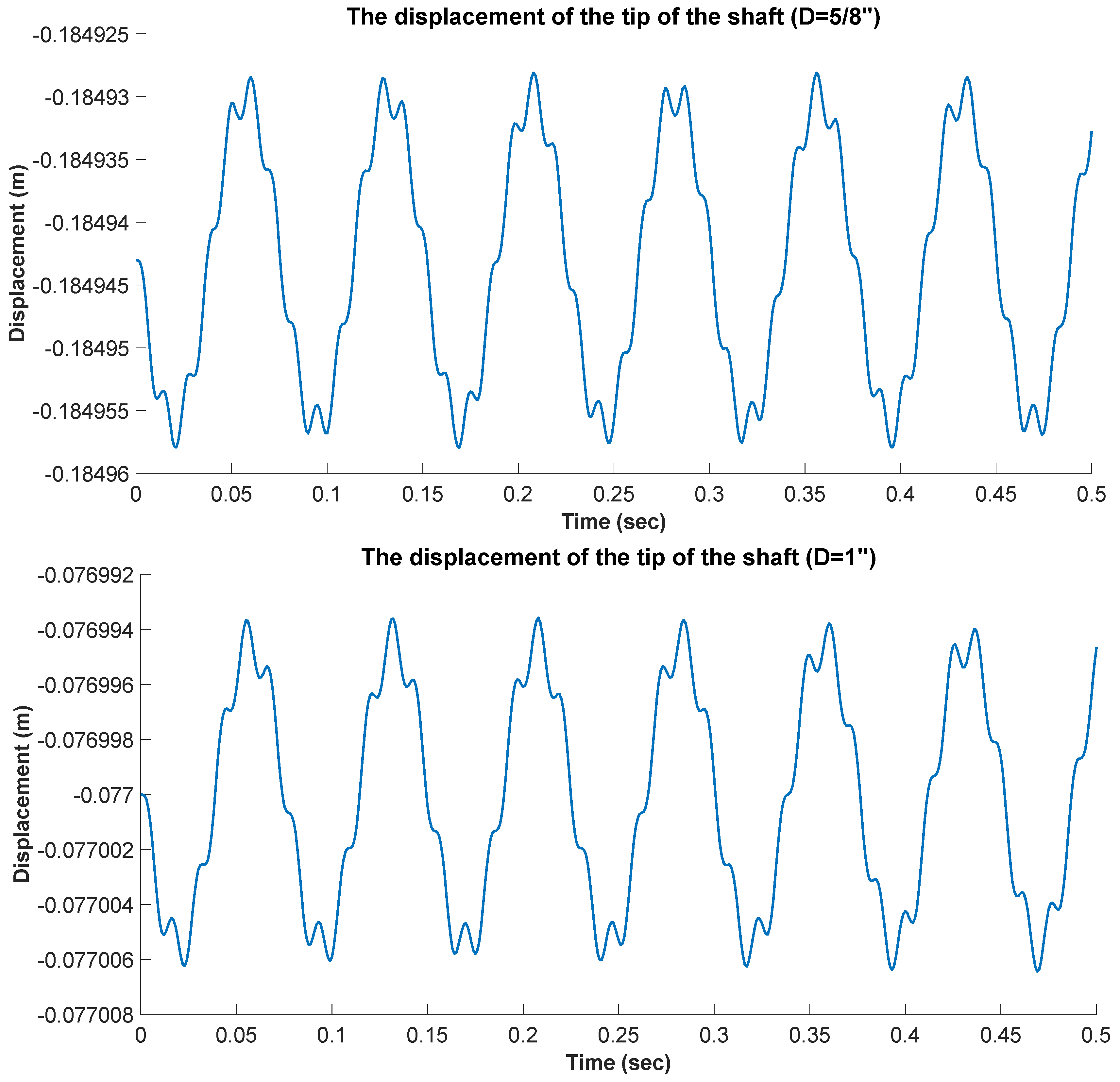
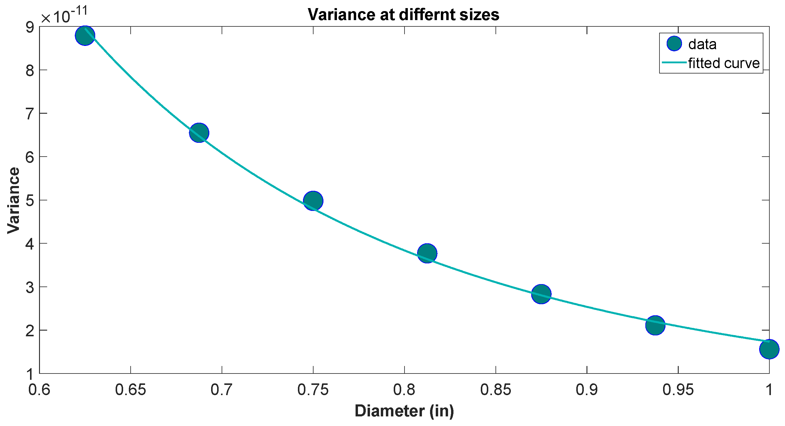
Another factor that can be examined is the shaft diameter. As shown in Figure 18, altering the shaft diameter affects the displacement amplitude. The results indicate that as the shaft diameter increases, the output amplitude also rises, a pattern that is further supported by statistical analysis. Figure 19 demonstrates that a larger shaft diameter leads to a reduction in data variance, which is consistent with the observed increase in response amplitude.

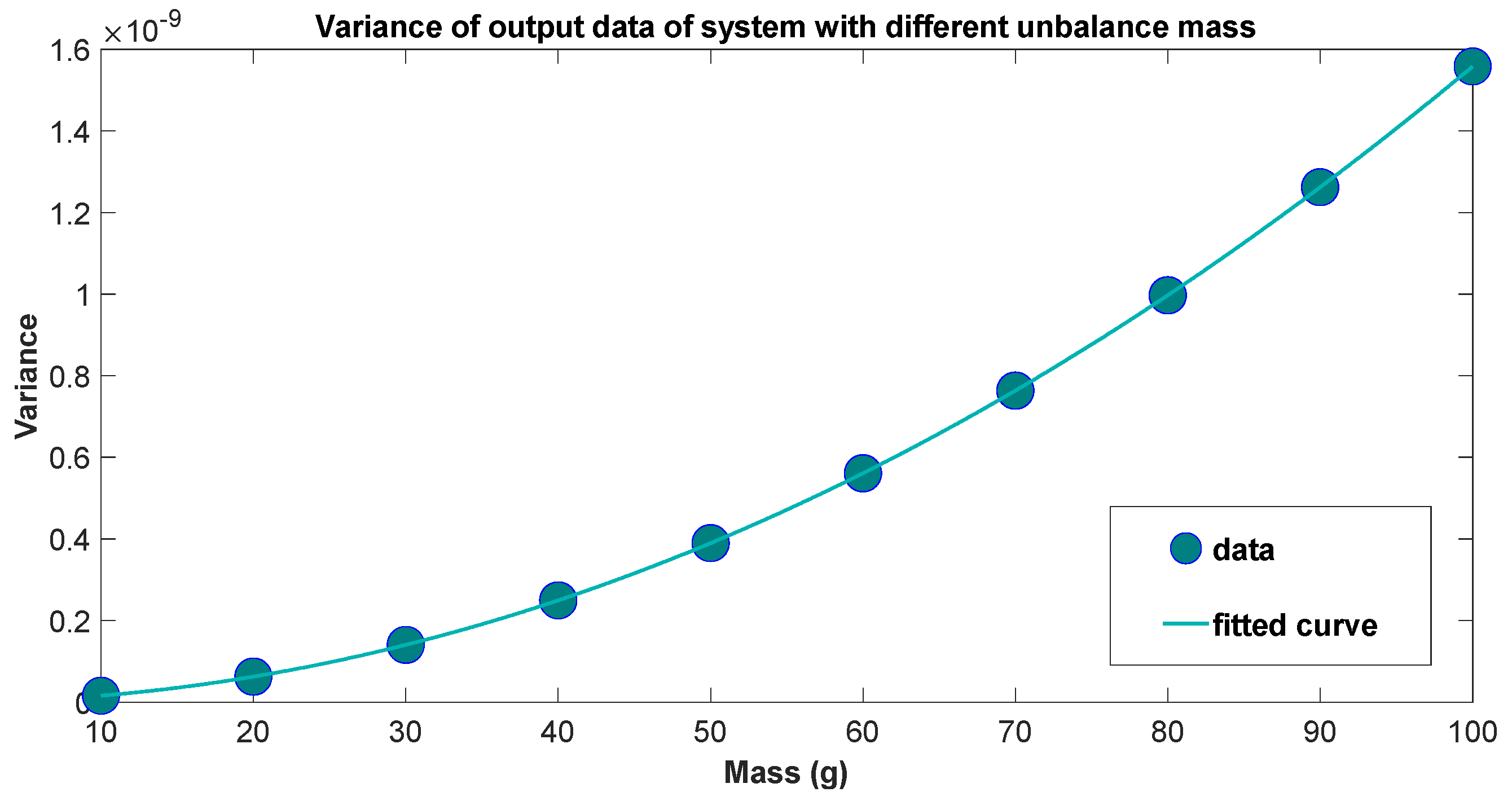
Finally, the last parameter considered was the magnitude of unbalance, i.e., the mass and radial distance. In this case, the mass was changed, and the radial distance was kept at 10 mm. The results obtained are presented in Figure 20. Variance rises as unbalance increases.

So far, it has been established that the SSD delivers modal and transient results that are on par with those generated by existing commercial software packages. While the SSD simulations may not achieve the same level of detail as FEA programs, accuracy is not their primary strength. Instead, the key advantage of SSD lies in its ability to quickly generate extensive datasets of defective cases with sufficient accuracy. This capability is particularly valuable for the implementation of LIVE DT.

The LF software operates at a much higher speed compared to traditional FEA tools. For instance, simulating the rotary machine examined in this study required around 3 min using standard commercial programs, whereas SSD processed each scenario in under a second. Although this time difference might seem negligible initially, it becomes indispensable when constructing extensive datasets for training machine learning models.

During the verification stage of the LIVE DT methodology, a critical task involves generating a vast collection of different samples. These samples could represent rotary systems with components experiencing varying levels of damage (i.e., reductions in stiffness). By considering just five defect types, as shown in Figure 11, and assuming stiffness losses of 0%, 25%, 50%, and 75%, a substantial number of fault scenarios can be created (4⁷ = 16,384). This comprehensive dataset can then be utilized to train an algorithm capable of evaluating a system’s condition based on its dynamic response or forecasting its future state and performance. Creating such a large dataset using conventional FEA tools is computationally intensive; generating 16,384 scenarios would take approximately 34 days (more than one month), whereas SSD can accomplish the same task in under five hours.

The speed of LF simulations also supports real-time and instantaneous analysis of a machine’s condition. This allows for continuous online monitoring, enabling timely corrective actions when required.

Furthermore, the LF method is highly versatile and customizable, enabling adjustments to key parameters to better replicate the behavior of high-fidelity models or real-world systems. Machine learning techniques can also be applied to refine the SSD program, enhancing its ability to deliver more precise and reliable outcomes. In contrast, commercial software packages often function as black boxes, offering limited customization options.

4. Conclusions

This paper presented the development of Simple Structural Dynamics (SSD), a computationally efficient Low-Fidelity (LF) simulation designed for integration into the LIVE Digital Twin methodology for rotary machinery. The principal contribution of Simple Structural Dynamics is its ability to combine modal and transient analyses. In contrast to earlier low-fidelity approaches, such as Simple Structural Beams, which were primarily limited to static and modal analysis, Simple Structural Dynamics incorporates consistent mass and stiffness formulations together with Newmark’s time-integration method to generate both frequency-domain and time-domain responses.

The proposed framework was evaluated using a rotor–bearing–flywheel case study under healthy and unhealthy operating conditions. The results showed that Simple Structural Dynamics can reproduce the principal dynamic characteristics of the system, including natural frequencies, mode shapes, and transient displacement responses, with reasonable agreement relative (less than 6% difference in first 10 natural frequencies and less than 1% difference in mean and variance of the displacement data) to a commercial high-fidelity finite element model. Mesh refinement substantially reduced the differences in the higher natural frequencies, while the remaining discrepancy was attributed mainly to the inherent model-form differences between the simplified beam-and-spring representation and the detailed three-dimensional High-Fidelity (HF) model.

The study also demonstrated the ability of Simple Structural Dynamics to represent common rotary-machine faults. Shaft cracks and bearing defects were introduced through localized stiffness reductions, while flywheel unbalance was represented by eccentric dynamic loading. The results showed that stiffness degradation generally reduced the natural frequencies and altered the transient response, whereas increasing unbalance, shaft speed, and selected geometric parameters produced measurable changes in displacement and statistical indicators. These findings confirm that Simple Structural Dynamics outputs can provide useful information for condition monitoring and fault diagnosis.

A key advantage of Simple Structural Dynamics is its computational efficiency. While a comparable commercial finite element simulation required several minutes, Simple Structural Dynamics completed each case in less than one second. This speed makes it practical to generate the large datasets required for machine-learning-based fault diagnosis and for real-time applications within the Verify stage of LIVE Digital Twin. The open and customizable structure of Simple Structural Dynamics also allows model parameters to be calibrated against High-Fidelity or experimental data, improving its representation of the physical system.

This study represents the first stage of a broader research program aimed at developing Digital Twins for rotary machinery. The present rotor–bearing–flywheel assembly serves as an initial case study for establishing and validating the Simple Structural Dynamics methodology. Future research will extend the framework to more complex rotary systems, additional machine components such as couplings and gear assemblies, a broader range of fault modes, experimental calibration, and machine-learning-based diagnosis and prognosis. These developments will further support the integration of Simple Structural Dynamics into a complete LIVE Digital Twin capable of real-time health monitoring, Remaining Useful Life (RUL) estimation, and predictive maintenance decision-making.

References

1. Singh, R.R.; Bhatti, G.; Kalel, D.; Vairavasundaram, I.; Alsaif, F. Building a Digital Twin Powered Intelligent Predictive Maintenance System for Industrial AC Machines. Machines 2023, 11, 796. [Google Scholar] [CrossRef]
2. Nozari, H.; Szmelter-Jarosz, A. A Predictive Maintenance Approach for Composting Plants Based on ERP and Digital Twin Integration. Machines 2025, 13, 1123. [Google Scholar] [CrossRef]
3. Dini, P.; Nardi, D.; Saponara, S. Overview on Predictive Maintenance Techniques for Turbomachinery. Machines 2026, 14, 396. [Google Scholar] [CrossRef]
4. You, Y.; Chen, C.; Hu, F.; Liu, Y.; Ji, Z. Advances of digital twins for predictive maintenance. Procedia Comput. Sci. 2022, 200, 1471–1480. [Google Scholar] [CrossRef]
5. Luo, W.; Hu, T.; Ye, Y.; Zhang, C.; Wei, Y. A hybrid predictive maintenance approach for CNC machine tool driven by Digital Twin. Robot. Comput.-Integr. Manuf. 2020, 65, 101974. [Google Scholar] [CrossRef]
6. Aivaliotis, P.; Georgoulias, K.; Chryssolouris, G. The use of Digital Twin for predictive maintenance in manufacturing. Int. J. Comput. Integr. Manuf. 2019, 11, 1067–1080. [Google Scholar] [CrossRef]
7. Liu, M.; Fang, S.; Dong, H.; Xu, C. Review of digital twin about concepts, technologies, and industrial applications. J. Manuf. Syst. 2021, 58, 346–361. [Google Scholar] [CrossRef]
8. Gunasegaram, D.R.; Murphy, A.B.; Barnard, A.; DebRoy, T.; Matthews, M.J.; Ladani, L.; Gu, D. Towards developing multiscale-multiphysics models and their surrogates for digital twins of metal additive manufacturing. Addit. Manuf. 2021, 46, 102089. [Google Scholar] [CrossRef]
9. Mahmoodian, M.; Shahrivar, F.; Setunge, S.; Mazaheri, S. Development of digital twin for intelligent maintenance of civil infrastructure. Sustainability 2022, 14, 8664. [Google Scholar] [CrossRef]
10. Yakhni, M.F.; Hosni, H.; Cauet, S.; Sakout, A.; Etien, E.; Rambault, L.; Assoum, H.; El-Gohary, M. Design of a digital twin for an industrial vacuum process: A predictive maintenance approach. Machines 2022, 10, 686. [Google Scholar] [CrossRef]
11. Tao, F.; Zhang, M.; Liu, Y.; Nee, A.Y. Digital twin driven prognostics and health management for complex equipment. Cirp Ann. 2018, 1, 169–172. [Google Scholar] [CrossRef]
12. Grieves, M. Digital twin: Manufacturing excellence through virtual factory replication. White Pap. 2014, 1, 1–7. [Google Scholar]
13. Liu, Z.; Chen, W.; Zhang, C.; Yang, C.; Chu, H. Data super-network fault prediction model and maintenance strategy for mechanical product based on digital twin. IEEE Access 2019, 7, 177284–177296. [Google Scholar] [CrossRef]
14. Nagurney, A.; Wakolbinger, T. Supernetworks: An introduction to the concept and its applications with a specific focus on knowledge supernetworks. Int. J. Knowl. Cult. Change Manag. 2005, 4, 1–16. [Google Scholar] [CrossRef]
15. Juarez, M.G.; Botti, V.J.; Giret, A.S. Digital twins: Review and challenges. J. Comput. Inf. Sci. Eng. 2021, 21, 030802. [Google Scholar] [CrossRef]
16. Xiong, M.; Wang, H.; Fu, Q.; Xu, Y. Digital twin–driven aero-engine intelligent predictive maintenance. Int. J. Adv. Manuf. Technol. 2021, 114, 3751–3761. [Google Scholar]
17. Booyse, W.; Wilke, D.N.; Heyns, S. Deep digital twins for detection, diagnostics and prognostics. Mech. Syst. Signal Process. 2020, 140, 106612. [Google Scholar] [CrossRef]
18. Çınar, Z.M.; Abdussalam Nuhu, A.; Zeeshan, Q.; Korhan, O.; Asmael, M.; Safaei, B. Machine learning in predictive maintenance towards sustainable smart manufacturing in industry 4.0. Sustainability 2020, 12, 8211. [Google Scholar] [CrossRef]
19. Malek, N.G.; Tayefeh, M.; Bender, D.; Barari, A. Live digital twin for smart maintenance in structural systems. IFAC-PapersOnLine 2021, 1, 1047–1052. [Google Scholar] [CrossRef]
20. Bondoc, A.E.; Tayefeh, M.; Barari, A. Employing LIVE digital twin in prognostic and health management: Identifying location of the sensors. IFAC-PapersOnLine 2022, 2, 138–143. [Google Scholar] [CrossRef]
21. Tebby, S.; Barari, A.; Esmailzadeh, E. Development of optimized preliminary vehicle structural model using simple structural beams-frames (ssb) and sub-structural analysis. Comput.-Aided Des. Appl. 2014, 5, 544–551. [Google Scholar] [CrossRef]
22. Asbaghian Namin, S.F.; Barari, A. Low Fidelity Simulation in LIVE Digital Twin to Detect Rotational Errors in Production Machinery. IFAC-PapersOnLine 2026, 59, 149–154. [Google Scholar]
23. Chandrupatla, T.R.; Belegundu, A.D.; Ramesh, T.; Ray, C. Introduction to Finite Elements in Engineering; Pearson: London, UK, 2012. [Google Scholar]
24. Logan, D.L. A First Course in the Finite Element Method; Thomson: Belmont, CA, USA, 2011; Volume 4. [Google Scholar]
25. Rao, S.S. Vibration of Continuous Systems; John Wiley & Sons: Hoboken, NJ, USA, 2019. [Google Scholar]
26. Ellman, A.; Pajunen, S.; Laine, I.; Coatanea, E. Engineering Design Analysis Tool for Early Design Phase With Low-Fidelity Models: A Case of Hydraulic Crane. In International Design Engineering Technical Conferences and Computers and Information in Engineering Conference; American Society of Mechanical Engineers: New York, NY, USA, 2017; p. V001T002A017. [Google Scholar]
27. Wood, I.; Barari, A.; Esmailzadeh, E. Using the simple structural beam model to optimize and analyze automotive structures for torsion stiffness and fundamental natural frequency. In Canadian Society for Mechanical Engineering International Congress; American Society of Mechanical Engineers: New York, NY, USA, 2014. [Google Scholar]
28. Gomes, G.F.; de Almeida, F.A.; da Silva Lopes Alexandrino, P.; da Cunha, S.S.; de Sousa, B.S.; Ancelotti, A.C. A multiobjective sensor placement optimization for SHM systems considering Fisher information matrix and mode shape interpolation. Eng. Comput. 2019, 35, 519–535. [Google Scholar]
29. Tygesen, U.T.; Jepsen, M.S.; Vestermark, J.; Dollerup, N.; Pedersen, A. The true digital twin concept for fatigue re-assessment of marine structures. In International Conference on Offshore Mechanics and Arctic Engineering; American Society of Mechanical Engineers: New York, NY, USA, 2018; Volume 51203, p. V001T01A021. [Google Scholar]
30. James, M.L.; Smith, G.M.; Wolford, J.C. Applied Numerical Methods for Digital Computation; Addison-Wesley Longman Publishing Co., Inc.: Boston, MA, USA, 1984. [Google Scholar]
31. Newmark, N.M. A method of computation for structural dynamics. J. Eng. Mech. Div. 1959, 85, 67–94. [Google Scholar] [CrossRef]
32. Bathe, K.J.; Wilson, E.L. Numerical Methods in Finite Element Analysis; Prentice-Hall: Englewood Cliffs, NJ, USA, 1976. [Google Scholar]
33. Houbolt, J.C. A recurrence matrix solution for the dynamic response of elastic aircraft. J. Aeronaut. Sci. 1950, 17, 540–550. [Google Scholar] [CrossRef]
34. Brandt, A. Noise and Vibration Analysis: Signal Analysis and Experimental Procedures; John Wiley & Sons: Hoboken, NJ, USA, 2023. [Google Scholar]
Figure 1. An illustrative example of FWD simulation.
Machines 14 00737 g001
Figure 2. Visualization of BWD simulation in a clamped beam.
Machines 14 00737 g002
Figure 3. Comparison of HF and LF simulations: (a) the physical system represented by a clamped beam loaded at one end; (b) the corresponding high-fidelity model; and (c) the simplified low-fidelity model.
Machines 14 00737 g003
Figure 4. Four main steps of Live DT approach [19].
Machines 14 00737 g004
Figure 5. The experimental setup.
Machines 14 00737 g005
Figure 6. The SSD counterpart of the experimental setup.
Machines 14 00737 g006
Figure 7. The configuration of rotary system in the commercial FEM program.
Machines 14 00737 g007
Figure 8. The equivalent SSD model of the rotary machine.
Machines 14 00737 g008
Figure 9. Node interpolation.
Machines 14 00737 g009
Figure 10. Healthy system mode shapes at various frequencies.
Machines 14 00737 g010
Figure 11. SSD model of the defective rotary machine.
Machines 14 00737 g011
Figure 12. The effect of shaft diameter on fundamental frequency.
Machines 14 00737 g012
Figure 13. A comparison of displacement results produced by the SSD and FEA software.
Machines 14 00737 g013
Figure 14. The graphical representation of the shaft after 0.5 s.
Machines 14 00737 g014
Figure 15. Depicting the impact of faulty components on the displacement.
Machines 14 00737 g015
Figure 16. The displacement of the tip of the shaft at different speeds.
Machines 14 00737 g016
Figure 17. The effect of rotational speed of the shaft on the crest of the collected transient data.
Machines 14 00737 g017
Figure 18. The displacement of the tip of the shaft with different diameters.
Machines 14 00737 g018
Figure 19. The effect of shaft diameter on the variance of collected transient data.
Machines 14 00737 g019
Figure 20. The effect of unbalance mass on the variance of collected transient data.
Machines 14 00737 g020