A Short-Circuit Fault Diagnosis Method for Three-Phase Current-Source Inverters Using Normalized Phase Current Variation Trends

Abstract

This paper presents a fast diagnosis and localization method for switch short-circuit faults (shoot-through faults) in three-phase current-source inverters (CSIs) based on the polarity and variation trends of normalized phase currents. Under short-circuit fault conditions, the variation trends of the two same-polarity phase currents change from opposite (normal) to identical. To capture this feature, an adaptive magnitude-normalization method is proposed, which adaptively distinguishes normal load variations from fault conditions and selects the corresponding normalization strategy, yielding constant-amplitude three-phase currents while retaining polarities and trends. The theoretical operating sector is determined from the current polarities, and the faulty switch is localized using the signs of the variation trends of the two same-polarity currents. The method applies to both single- and multiple-switch faults. Experiments on a 3 A, 50 Hz CSI prototype show an average localization time of 15 ms (0.75$T_{\mathrm{base}}$), accurate diagnosis under load (10–30 $\Omega$) and frequency (25–50 Hz) variations, and no need for additional hardware, confirming its effectiveness.

1. Introduction

Three-phase current-source inverters (CSIs) are widely used in AC motor drives [1,2,3] and renewable energy generation systems [4,5]. The reliable operation of CSIs is critical to the safe operation of the aforementioned systems. Performing fault diagnosis and localization followed by fault-tolerant system control can significantly enhance the operational reliability of the inverters [6]. Therefore, it is necessary to conduct in-depth research on fault diagnosis methods for switching devices in CSIs.

At present, switching-device faults of inverters are classified into open-circuit faults (OCFs) and short-circuit faults (SCFs). SCFs in voltage-source inverters (VSIs) and OCFs in CSIs exhibit obvious characteristics and present severe hazards, requiring immediate isolation. In contrast, OCFs in VSIs and SCFs in CSIs show indistinct features, yet their long-term existence tends to induce secondary faults. Therefore, it is necessary to extract fault characteristics beyond overcurrent and overvoltage to achieve fault diagnosis and localization [7].

Existing research mainly focuses on OCFs in VSIs, while studies on diagnostic methods for SCFs of switching devices in CSIs are relatively limited [8]. However, VSIs and CSIs share similar topological constraints. This enables diagnostic methods for OCFs of switching devices in VSIs to provide references for the development of fault diagnosis methods for SCFs of switching devices in CSIs [9].

At present, fault diagnosis methods for inverters can be categorized into two types: methods based on switching-device fault characteristics and methods based on circuit topology constraints. Methods based on switching-device fault characteristics can achieve fast diagnosis. For example, Ref. [10] proposes a diagnostic algorithm that detects IGBT open-circuit faults by measuring only the gate voltage. In [11], a diagnostic algorithm based on the internal gate state of a MOSFET is proposed to detect short-circuit faults. Ref. [12] proposes a diagnostic algorithm for MOSFET short-circuit faults based on indirect power level. These algorithms have very short diagnosis times and are not affected by load conditions; however, they require additional sampling circuits for the switching devices, which increases diagnostic cost and introduces new potential failure points.

Methods based on fault characteristics derived from circuit topology constraints are mainly are divided into two types: voltage-based methods and current-based methods. At present, diagnostic methods based on voltage signals mainly focus on OCFs of VSIs. Ref. [13] proposes an OCF diagnostic method based on zero-sequence voltage components. An adjacent-trend-line method was proposed in [14] for inverter open-circuit fault diagnosis. An OCF diagnostic method for the output line voltage model is presented in [15]. Ref. [16] proposed a normalization-based OC fault diagnosis method using a sliding window, DFT, and PCA. Regarding current diagnostic methods for SCFs in CSI switching devices, a hybrid diagnostic method based on capacitor voltage and equivalent duty cycle logic derivation is proposed in [17]. These methods are efficient and accurate, enabling rapid fault localization within less than one fundamental cycle. However, these methods inevitably require additional voltage sampling circuits, which also increase the cost and system complexity.

Current fault diagnosis methods based on current signals mainly focus on open-circuit faults of switching devices in voltage-source inverters (VSIs). In [18], the different current vector trajectories caused by different switching devices are used to diagnose and locate the faulty switch. In [19], the main fault characteristics of three-phase current after an open-circuit fault are identified as being concentrated in the low-frequency band, enabling fault location. In [20], fault characteristics of abnormal current patterns caused by open-circuit faults are extracted to locate the faulty switch. In [21], fault characteristics of phase angle signal anomalies caused by open-circuit faults are extracted to locate the faulty switch. To date, studies on switching-device SCFs diagnosis for CSIs based on current signals remain limited. In [22], a diagnostic variable is derived by calculating the ratio between the average feedback current over one power-frequency cycle and the average absolute value of the current reference signal, thereby identifying the faulty switching device. In [23], the current modulus following Clarke transformation of three-phase currents is evaluated. Fault localization is then achieved by combining the characteristic-zero current modulus induced by a short-circuit fault with phase angle signal information. Although these methods eliminate the need for additional sampling circuits, their diagnostic response time is relatively slow.

Currently, diagnostic methods based on current signals for SCFs of switching devices in CSIs have relatively long diagnosis times [22,23]. Methods that enable fast diagnosis and localization require additional voltage sampling circuits [17]. Therefore, this paper proposes a diagnostic method that does not require additional sampling circuits and can quickly diagnose and locate the faulty switching device. The method is based on the polarity and variation trends of phase currents as fault characteristics for diagnosing and locating a single faulty switch in a CSI. The main contributions of this paper are as follows:

• The variation trends and polarities of three-phase currents under normal and abnormal conditions are qualitatively analyzed to identify a fault characteristic: for an SCF, two phase currents with the same polarity exhibit identical variation trends.
• An adaptive normalization method for variable-load conditions is proposed. Through mode switching, the proposed method suppresses the amplitude variation caused by load changes while preserving the structural abnormality associated with the fault, thereby providing a stable input for subsequent fault diagnosis.
• A fault diagnosis method based on three-phase current polarity and current variation trends is proposed. The proposed fault diagnosis method can accurately locate the faulty switch and maintains high robustness under operating conditions with continuously varying output-current magnitude and frequency.

The remainder of this paper is organized as follows. Section 2 introduces the three-phase current-source inverter system and the polarity and variation trends of three-phase currents under normal operating conditions. Section 3 analyzes the influence of single-switch faults on the polarity and variation trends of three-phase currents. An algorithm based on current polarity and variation trends is proposed to suppress current ripple and noise interference, and a fault diagnosis and localization method using these fault characteristics is presented. Section 4 verifies the proposed method through experiments. Section 5 concludes this paper. Section 6 discusses the limitations of this method and directions for further research.

2. Analysis of SCFs in a CSI

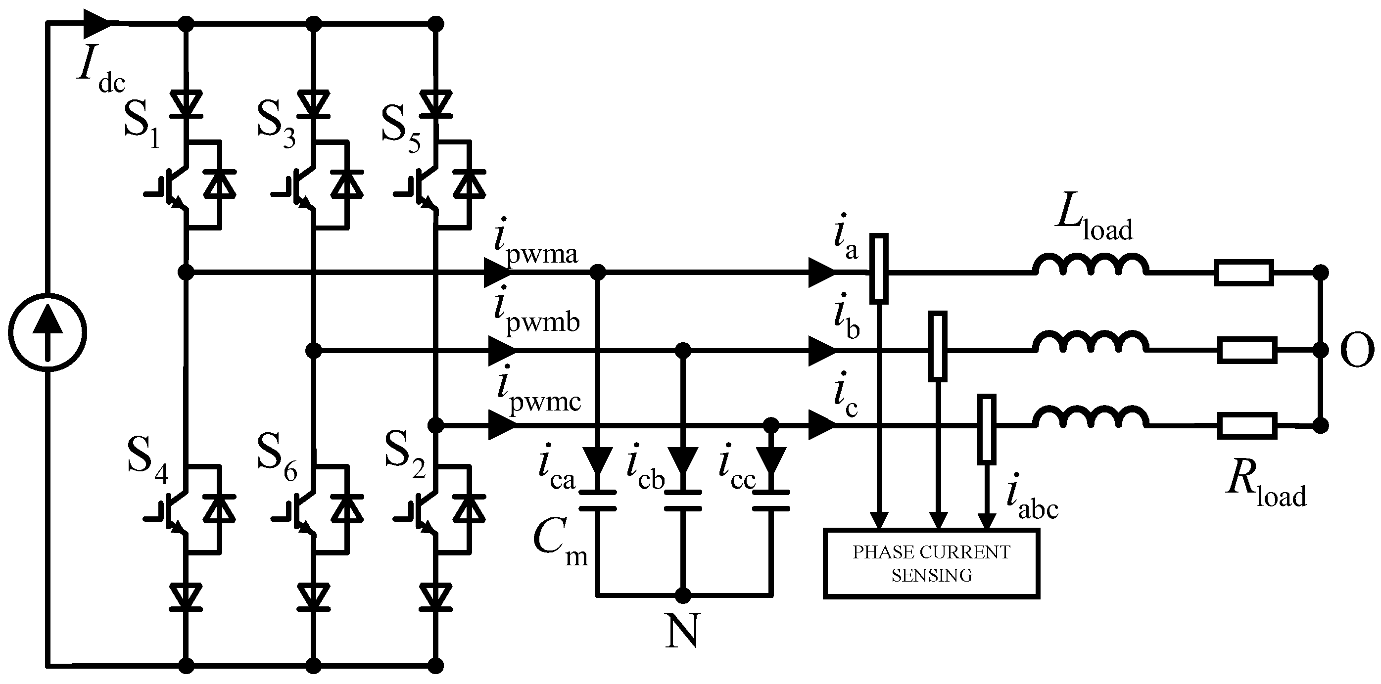
Figure 1 shows the topology of a three-phase current-source inverter. The DC side outputs a constant current $I_{dc}$. Its core consists of six IGBT switching devices connected in series with diodes (${\mathrm{S}}_1$–${\mathrm{S}}_6$). High-frequency pulse current is supplied to the load via specific switching operations. The capacitor $C_m$ acts as a filter to provide a sinusoidal current for the load ($R_{load}$ and $L_{load}$).

Space vector pulse width modulation (SVPWM) controls the IGBT switches. The relationship between the load current vector and the three-phase load current can be stated as

$$I\left(t\right)={\displaystyle \frac{2}{3}}\left[i_{\mathrm{a}}+i_{\mathrm{b}}{e}^{j{\displaystyle \frac{2}{3}}\pi }+i_{\mathrm{c}}{e}^{j{\displaystyle \frac{4}{3}}\pi }\right]$$

(1)

The PWM switching mode for the CSI requires only two switches to conduct simultaneously at any given time: one in the top half of the CSI bridge and the other in the bottom half. Three-phase CSIs have nine switching states, and the corresponding state table is

Table 1. Normal-state correspondence between switching states and three-phase currents.

Space Vector	Switching States	${\mathbf{i}}_{\mathit{a}}$	${\mathbf{i}}_{\mathit{b}}$	${\mathbf{i}}_{\mathit{c}}$
${\mathit{I}}_1$	${\mathrm{S}}_6$ and ${\mathrm{S}}_1$	${\mathrm{I}}_{dc}$	−${\mathrm{I}}_{dc}$	0
${\mathit{I}}_2$	${\mathrm{S}}_1$ and ${\mathrm{S}}_2$	${\mathrm{I}}_{dc}$	0	−${\mathrm{I}}_{dc}$
${\mathit{I}}_3$	${\mathrm{S}}_2$ and ${\mathrm{S}}_3$	0	${\mathrm{I}}_{dc}$	−${\mathrm{I}}_{dc}$
${\mathit{I}}_4$	${\mathrm{S}}_3$ and ${\mathrm{S}}_4$	−${\mathrm{I}}_{dc}$	${\mathrm{I}}_{dc}$	0
${\mathit{I}}_5$	${\mathrm{S}}_4$ and ${\mathrm{S}}_5$	−${\mathrm{I}}_{dc}$	0	${\mathrm{I}}_{dc}$
${\mathit{I}}_6$	${\mathrm{S}}_5$ and ${\mathrm{S}}_6$	0	−${\mathrm{I}}_{dc}$	${\mathrm{I}}_{dc}$
${\mathit{I}}_7$	${\mathrm{S}}_1$ and ${\mathrm{S}}_4$	0	0	0
${\mathit{I}}_8$	${\mathrm{S}}_3$ and ${\mathrm{S}}_6$	0	0	0
${\mathit{I}}_9$	${\mathrm{S}}_5$ and ${\mathrm{S}}_2$	0	0	0

:

By substituting the three-phase current relationships corresponding to the switching states into (1), the load space current vector diagram under normal switching states can be obtained.

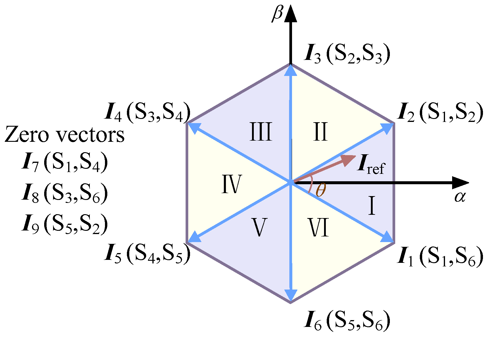
For example, when ${\mathrm{S}}_1$ and ${\mathrm{S}}_6$ are conducting, $i_a=I_{dc}$, $i_b=-I_{dc}$, and $i_c=0$. Substituting these into (1) yields ${\mathit{I}}_1=2/\sqrt{3}{I}_{dc}{e}^{-j\pi /6}$. By repeating the above calculation process, all active vectors ${\mathit{I}}_1$–${\mathit{I}}_6$ and zero vectors ${\mathit{I}}_7$–${\mathit{I}}_9$ in normal working conditions can be obtained in Figure 2. The reference current vector ${\mathit{I}}_{\mathrm{ref}}$ is obtained by controlling the on/off time of two adjacent active current vectors and one zero current vector through SVPWM. $\theta$ is the angle between the reference vector and the starting boundary of the sector.

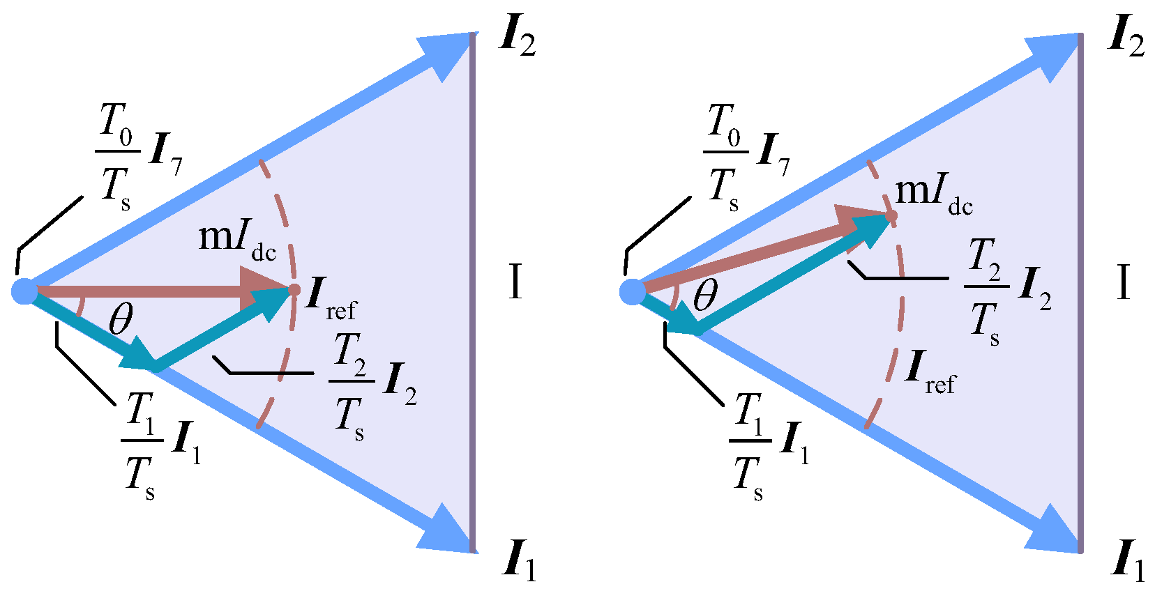
When the reference vector ${\mathit{I}}_{ref}$ rotates into Sector I, the active vectors are ${\mathit{I}}_1$ and ${\mathit{I}}_2$, and the zero vector is ${\mathit{I}}_7$. According to the ampere-second balance principle, the dwell times of the corresponding vectors are $T_1$, $T_2$, and $T_0$.

$${\mathit{I}}_{\mathrm{ref}}={\mathit{I}}_1{\displaystyle \frac{T_1}{T_{\mathrm{s}}}}+{\mathit{I}}_2{\displaystyle \frac{T_2}{T_{\mathrm{s}}}}+{\mathit{I}}_7{\displaystyle \frac{T_0}{T_{\mathrm{s}}}}$$

(2)

where $T_s$ is the switching period.

$$\left\{\begin{array}{c}{T}_1=T_{\mathrm{s}}·m_s·\sin \left(\pi /3-\theta \right)\hfill \\ T_2=T_{\mathrm{s}}·m_s·\sin \left(\theta \right)\hfill \\ T_0=T_{\mathrm{s}}-T_1-T_2\hfill \end{array}\right.0<\theta \le \pi /3$$

(3)

Owing to sector symmetry, the dwell times of the corresponding vectors in all sectors satisfy the same relationship.

The dwell times of the two active vectors affect the equivalent area of the high-frequency PWM output and, thus, the magnitudes of the three-phase currents at the corresponding instants. Under normal operation, the dwell times are related to the rotational speed of the reference vector, which equals the load-side operating frequency. The frequency of three-phase load currents can be utilized to qualitatively indicate the dynamic variation in voltage vector dwell time during operation.

$$0<\theta =2\pi ft\le \pi /3$$

(4)

where f is the load-side current frequency and t is the operating time of the reference vector within the corresponding sector.

Combined with the switching states of active vectors in the sector of the reference vector, both the polarity and the variation trend in three-phase load currents can be qualitatively analyzed. Taking Sector I as an example, the dwell time of vector ${\mathit{I}}_1$ gradually decreases while that of vector ${\mathit{I}}_2$ increases, as shown in Figure 3.

The expressions for the three-phase currents in Sector I can be derived from the conduction states of ${\mathit{I}}_1$, ${\mathit{I}}_2$ and the variation in their dwell times.

$$\left\{\begin{array}{c}{i}_a=m{I}_{dc}\sin (\pi /3+2\pi ft)\hfill \\ i_b=-m{I}_{dc}\sin (\pi /3-2\pi ft)\hfill \\ i_c=-m{I}_{dc}\sin \left(2\pi ft\right)\hfill \end{array}\right.$$

(5)

Thus, in Sector I, $i_a$ is always positive and has the largest magnitude, while $i_b$ and $i_c$ are opposite in polarity to $i_a$.

The variation trends of the three-phase currents can be obtained by differentiating the three-phase currents.

$$\left\{\begin{array}{c}{\displaystyle \frac{d{i}_a}{dt}}=2\pi fm{I}_{dc}\cos (\pi /3+2\pi ft)\hfill \\ {\displaystyle \frac{d{i}_b}{dt}}=2\pi fm{I}_{dc}\cos (\pi /3-2\pi ft)\hfill \\ {\displaystyle \frac{d{i}_c}{dt}}=-2\pi fm{I}_{dc}\cos \left(2\pi ft\right)\hfill \end{array}\right.$$

(6)

In Sector I, the variation trend of $i_a$ is first positive and then negative. $i_b$ is negative, but its variation trend is positive. $i_c$ is negative, and its variation trend is negative.

Repeating the above analysis yields the polarity and variation trend of three-phase currents at all instants under normal operation in

Table 2. Current polarities and variation trends in different sectors under normal conditions.

Origin Sector	${\mathbf{i}}_{\mathit{a}}$ Trend	${\mathbf{i}}_{\mathit{b}}$ Trend	${\mathbf{i}}_{\mathit{c}}$ Trend	Max-Phase Current Polarity
I		>0	<0	${\mathrm{i}}_a$ +Max
II	<0	>0		${\mathrm{i}}_c$ −Max
III	<0		>0	${\mathrm{i}}_b$ +Max
IV		<0	>0	${\mathrm{i}}_a$ −Max
V	>0	<0		${\mathrm{i}}_c$ +Max
VI	>0		<0	${\mathrm{i}}_b$ −Max

. Here, Max represents the phase current with the largest magnitude, and its sign indicates the current polarity. As derived previously, the maximum-magnitude phase current is opposite in polarity to the other two phases during sector operation, and so its polarity is denoted by $\pm Max$. In a normal sector, the same-polarity currents (i.e., the two phase currents with identical signs) exhibit opposite variation trends, where the variation trend is defined as the change in a current value from the previous moment to the current moment.

The combination of active vectors and the distribution of their conduction times during operation determine the polarity and variation trend of the three-phase currents.

3. Proposed Fault Diagnosis Algorithm

3.1. Analysis of Vector Angle Signal Characteristics Under Single-Switch SCFs

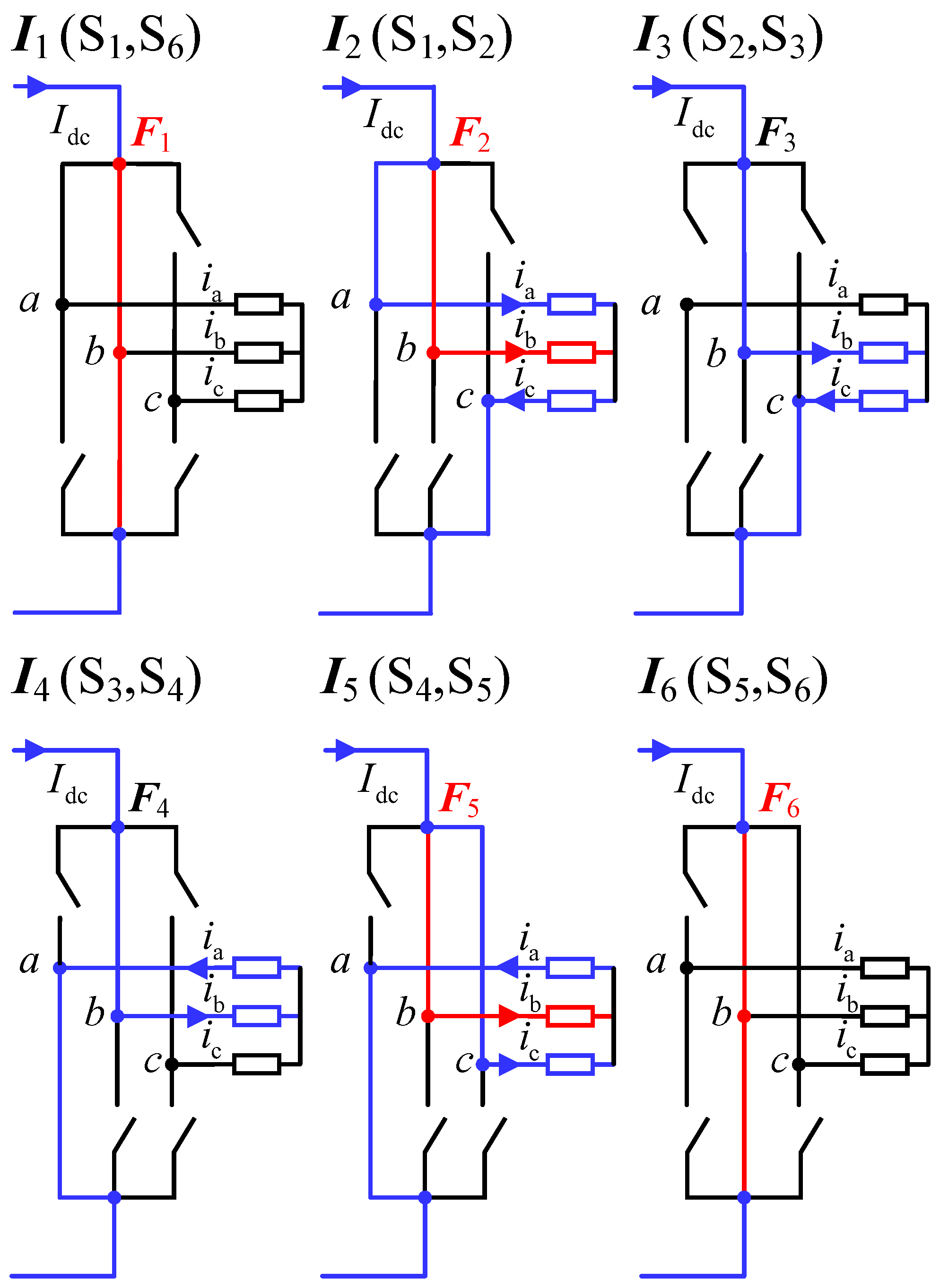
When ${\mathrm{S}}_3$ undergoes an SCF, the changes in the current corresponding to different current vectors are as shown in Figure 4. The output currents corresponding to the switching states after an SCF are shown in

Table 3. Faulty-state correspondence between switching states and three-phase currents when an SCF occurs in ${\mathrm{S}}_3$.

Space Vector	Faulty Switch	Switching States	${\mathbf{i}}_{\mathit{a}}$	${\mathbf{i}}_{\mathit{b}}$	${\mathbf{i}}_{\mathit{c}}$
${\mathit{I}}_1$	${\mathrm{S}}_3$	${\mathrm{S}}_6$ and ${\mathrm{S}}_1$	0	0	0
${\mathit{I}}_2$	${\mathrm{S}}_3$	${\mathrm{S}}_1$ and ${\mathrm{S}}_2$	1/2${\mathrm{I}}_{dc}$	1/2${\mathrm{I}}_{dc}$	−${\mathrm{I}}_{dc}$
${\mathit{I}}_3$	${\mathrm{S}}_3$	${\mathrm{S}}_2$ and ${\mathrm{S}}_3$	0	${\mathrm{I}}_{dc}$	−${\mathrm{I}}_{dc}$
${\mathit{I}}_4$	${\mathrm{S}}_3$	${\mathrm{S}}_3$ and ${\mathrm{S}}_4$	−${\mathrm{I}}_{dc}$	${\mathrm{I}}_{dc}$	0
${\mathit{I}}_5$	${\mathrm{S}}_3$	${\mathrm{S}}_4$ and ${\mathrm{S}}_5$	−${\mathrm{I}}_{dc}$	1/2${\mathrm{I}}_{dc}$	1/2${\mathrm{I}}_{dc}$
${\mathit{I}}_6$	${\mathrm{S}}_3$	${\mathrm{S}}_5$ and ${\mathrm{S}}_6$	0	0	0
${\mathit{I}}_7$	${\mathrm{S}}_3$	${\mathrm{S}}_1$ and ${\mathrm{S}}_4$	0	0	0
${\mathit{I}}_8$	${\mathrm{S}}_3$	${\mathrm{S}}_3$ and ${\mathrm{S}}_6$	0	0	0
${\mathit{I}}_9$	${\mathrm{S}}_3$	${\mathrm{S}}_5$ and ${\mathrm{S}}_2$	0	0	0

.

After an SCF of ${\mathrm{S}}_3$, the faulty switch creates a DC bypass via ${\mathit{I}}_1$ and ${\mathit{I}}_6$. In this switching state, all three phases’ load-side currents are zero. The faulty switch ${\mathrm{S}}_3$ also causes ${\mathit{I}}_2$ and ${\mathit{I}}_4$ to produce a state with all three phases conducting and two phases in parallel.

Consider Sector IV as an example. The expressions for the three phase currents in Sector IV can be derived from the conduction states of ${\mathit{I}}_6$ and ${\mathit{I}}_1$ and the variation in their dwell times. Thus, in Sector IV, $i_a=i_b=i_c=0$. At this time, the relative variation trend in the three phase currents is zero.

The expressions for the three phase currents in Sector I can be derived from the conduction states of ${\mathit{I}}_1$, ${\mathit{I}}_2$ and the variation in their dwell times.

$$\left\{\begin{array}{c}{i}_a=0.5m{I}_{dc}\sin \left(2\pi ft\right)\hfill \\ i_b=0.5m{I}_{dc}\sin \left(2\pi ft\right)\hfill \\ i_c=-m{I}_{dc}\sin \left(2\pi ft\right)\hfill \end{array}\right.$$

(7)

At this time, the three phase currents have a fixed proportional relationship. In Sector I, $i_c$ is always negative and has the largest magnitude, while $i_a$ and $i_b$ are opposite to $i_c$ in polarity. This is inconsistent with the polarity behavior of the three phase currents in normal Sector I.

The variation trends in the three phase currents can be obtained by differentiating these currents.

$$\left\{\begin{array}{c}{\displaystyle \frac{d{i}_a}{dt}}=\pi fm{I}_{dc}\cos \left(2\pi ft\right)\hfill \\ {\displaystyle \frac{d{i}_b}{dt}}=\pi fm{I}_{dc}\cos \left(2\pi ft\right)\hfill \\ {\displaystyle \frac{d{i}_c}{dt}}=-2\pi fm{I}_{dc}\cos \left(2\pi ft\right)\hfill \end{array}\right.$$

(8)

In Sector I, $i_a$ and $i_b$ are positive. The variation trends in $i_a$ and $i_b$ are positive. At this time, the variation trends in the two phase currents with the same polarity are no longer opposite but identical.

In Sector II, the expressions for the three phase currents can be derived from the conduction states of ${\mathit{I}}_2$ and ${\mathit{I}}_3$ and the variation in their dwell times.

$$\left\{\begin{array}{c}{i}_a=0.5m{I}_{dc}\sin (\pi /3-2\pi ft)\hfill \\ i_b={\displaystyle \frac{\sqrt{3}}{2}}m{I}_{dc}\sin (\pi /6+2\pi ft)\hfill \\ i_c=-m{I}_{dc}\sin (\pi /3+2\pi ft)\hfill \end{array}\right.$$

(9)

Thus, in Sector II, $i_c$ is always negative and has the largest magnitude, while $i_a$ and $i_b$ are opposite to $i_c$ in polarity. This is consistent with the polarity behavior of the three phase currents in normal Sector II.

The variation trends in the three phase currents can be obtained by differentiating these currents.

$$\left\{\begin{array}{c}{\displaystyle \frac{d{i}_a}{dt}}=-\pi fm{I}_{dc}\cos (\pi /3-2\pi ft)\hfill \\ {\displaystyle \frac{d{i}_b}{dt}}=\sqrt{3}\pi fm{I}_{dc}\cos (\pi /6+2\pi ft)\hfill \\ {\displaystyle \frac{d{i}_c}{dt}}=-2\pi fm{I}_{dc}\cos (\pi /3+2\pi ft)\hfill \end{array}\right.$$

(10)

In Sector II, the variation trend in $i_a$ is negative. However, the variation trend of $i_b$ is positive or zero.This is consistent with the variation trend behavior of the three phase currents in normal Sector II.

Repeating the above analysis process, when an SCF occurs in ${\mathrm{S}}_3$, the current polarities and variation trends for all sectors are as shown in

Table 4. Current polarities and variation trends in different sectors when an SCF occurs in ${\mathrm{S}}_3$.

Origin Sector	${\mathbf{i}}_{\mathit{a}}$ Trend	${\mathbf{i}}_{\mathit{b}}$ Trend	${\mathbf{i}}_{\mathit{c}}$ Trend	Max-Phase Current Polarity
I	>0	>0		${\mathrm{i}}_c$ − Max
II	<0	>0		${\mathrm{i}}_c$ −Max
III	<0		>0	${\mathrm{i}}_b$ +Max
IV		<0	>0	${\mathrm{i}}_a$ −Max
V		<0	<0	${\mathrm{i}}_a$ −Max
VI	=0	=0	=0	0

.

In summary, when an SCF occurs on a single switching device, the current polarities and variation trends in three sectors become abnormal.

$i_a=i_b=i_c=0$ is a common fault characteristic when an SCF occurs on a single switching device. For different short-circuit faults on a single switching device, the corresponding same-polarity, same-trend sectors are different. The corresponding current polarities and variation trends for the same-polarity, same-trend sectors are shown in

Table 5. Current polarities and variation trends in different SCF cases.

Faulty Tubes	DS	${\mathbf{i}}_{\mathit{a}}$ Trend	${\mathbf{i}}_{\mathit{b}}$ Trend	${\mathbf{i}}_{\mathit{c}}$ Trend	Max-Phase Current Polarity	Faulty Sector Output
S1	III	<0	<0		ic −Max	II
	V	>0		>0	ib −Max	VI
S2	IV	>0		>0	ib +Max	III
	VI		<0	<0	ia +Max	I
S3	I	>0	>0		ic −Max	II
	V		<0	<0	ia −Max	IV
S4	II	<0		<0	ib +Max	III
	VI	>0	>0		ic +Max	V
S5	I	<0		<0	ib −Max	VI
	III		>0	>0	ia −Max	IV
S6	II		>0	>0	ia +Max	I
	IV	<0	<0		ic +Max	V

.

3.2. Sliding-Window Sampling and Adaptive Magnitude-Normalization Mode Management

Normal load increase and load reduction cause significant variations in the overall amplitude of the three phase currents, which may interfere with the extraction of subsequent current-trend features. To reduce this influence, a method combining sliding-window sampling and adaptive magnitude normalization is adopted.

Let $f_s$ denote the sampling frequency and T denote the fundamental period. Then, the sliding-window length is defined as

$$N={\displaystyle \frac{1}{6}}{f}_{s}T.$$

(11)

At instant k, the three phase current windows are defined as

$$\begin{array}{cc}\hfill {\overrightarrow{I}}_a\left(k\right)& =\left[i_a(k-N+1),i_a(k-N+2),\dots ,i_a\left(k\right)\right],\hfill \\ \hfill {\overrightarrow{I}}_b\left(k\right)& =\left[i_b(k-N+1),i_b(k-N+2),\dots ,i_b\left(k\right)\right],\hfill \\ \hfill {\overrightarrow{I}}_c\left(k\right)& =\left[i_c(k-N+1),i_c(k-N+2),\dots ,i_c\left(k\right)\right].\hfill \end{array}$$

(12)

Accordingly, the three-phase sampled dataset at instant k is written as

$$\overrightarrow{I}\left(k\right)=\left[{\overrightarrow{I}}_a\left(k\right),{\overrightarrow{I}}_b\left(k\right),{\overline{I}}_c\left(k\right)\right].$$

(13)

On the basis of the three phase currents as sampled, the Clarke transformation yields

$$\left[\begin{array}{c}{i}_{\alpha }\left(k\right)\\ i_{\beta }\left(k\right)\end{array}\right]={\displaystyle \frac{2}{3}}\left[\begin{array}{ccc}1& -{\displaystyle \frac{1}{2}}& -{\displaystyle \frac{1}{2}}\\ 0& {\displaystyle \frac{\sqrt{3}}{2}}& -{\displaystyle \frac{\sqrt{3}}{2}}\end{array}\right]\left[\begin{array}{c}{i}_a\left(k\right)\\ i_b\left(k\right)\\ i_c\left(k\right)\end{array}\right],$$

(14)

The magnitude quantity and the local ratio quantity are further defined as

$$\mu \left(k\right)=\sqrt{i_{\alpha }^2\left(k\right)+i_{\beta }^2\left(k\right)},$$

(15)

$$q_{ab}\left(k\right)={\displaystyle \frac{|i_a\left(k\right)|}{|i_a\left(k\right)|+|i_b\left(k\right)|+\epsilon }}.$$

(16)

Here, $\epsilon$ is a small positive constant ($\epsilon =0.0001$) introduced to avoid division by zero.

Then, the corresponding magnitude window and ratio window are constructed as

$$\overrightarrow{M}\left(k\right)=\left[\mu (k-N+1),\mu (k-N+2),\dots ,\mu \left(k\right)\right].$$

(17)

$$\overrightarrow{Q}\left(k\right)=\left[q_{ab}(k-N+1),q_{ab}(k-N+2),\dots ,q_{ab}\left(k\right)\right].$$

(18)

$M\left(k\right)$ describes the temporal variation in the overall current magnitude, whereas $Q\left(k\right)$ describes the temporal variation in the local fixed-ratio relationship. The magnitude-related criterion and the structural criterion are subsequently constructed from $M\left(k\right)$ and $Q\left(k\right)$, respectively.

First, the last $L_p$ elements of $M\left(k\right)$ are used for short-term peak referencing, and the short-term peak reference is defined as

$${\mu }_{pk}\left(k\right)=\max \left[\mu (k-L_p+1),\dots ,\mu \left(k\right)\right].$$

(19)

Then, the magnitude-depth index and the variation-rate index are defined as

$$r\left(k\right)={\displaystyle \frac{\mu \left(k\right)}{{\mu }_{pk}\left(k\right)+\epsilon }},$$

(20)

$$d\left(k\right)={\displaystyle \frac{\left|\mu \right(k)-\mu (k-1\left)\right|}{{\mu }_{pk}\left(k\right)+\epsilon }}.$$

(21)

$r\left(k\right)$ reflects the reduction depth of the magnitude relative to the recent normal level, whereas $d\left(k\right)$ reflects the variation rate of the magnitude. Accordingly, the magnitude-related high-risk event is defined as

$$F_{\mu }\left(k\right)=\left\{\begin{array}{cc}1,\hfill & r\left(k\right)\le \gamma \mathrm{or}d\left(k\right)\ge \sigma ,\hfill \\ 0,\hfill & \mathrm{otherwise},\hfill \end{array}\right.$$

(22)

where $\gamma$ is the magnitude-depth threshold and $\sigma$ is the variation-rate threshold.

Second, within the last $L_f$ samples of $Q\left(k\right)$, the maximum and minimum values of the local ratio are defined as

$$q_{ab}^{\max }\left(k\right)=\max q_{ab}\left[\mu (k-L_p+1),\dots ,\mu \left(k\right)\right],$$

(23)

$$q_{ab}^{\min }\left(k\right)=\min q_{ab}\left[\mu (k-L_p+1),\dots ,\mu \left(k\right)\right],$$

(24)

$$V_{ab}\left(k\right)=q_{ab}^{\max }\left(k\right)-q_{ab}^{\min }\left(k\right).$$

(25)

Accordingly, the fixed-ratio structural high-risk event is defined as

$$F_p\left(k\right)=\left\{\begin{array}{cc}1,\hfill & F_{\mu }\left(k\right)=1\mathrm{and}{V}_{ab}\left(k\right)<\eta ,\hfill \\ 0,\hfill & \mathrm{otherwise},\hfill \end{array}\right.$$

(26)

where $\eta$ is the unified structural threshold. The near-zero counting variable is defined as

$$N_z\left(k\right)={\displaystyle \sum _{j=k-L_p+1}^k}\mathbf{1}\left({\displaystyle \frac{\mu \left(j\right)}{{\mu }_{pk}\left(k\right)+\epsilon }}<\eta \right),$$

(27)

where $\mathbf{1}(·)$ denotes the indicator function.

The near-zero collapse high-risk event is defined as

$$F_z\left(k\right)=\left\{\begin{array}{cc}1,\hfill & N_z\left(k\right)\ge {\displaystyle \frac{3}{5}}{L}_p,\hfill \\ 0,\hfill & \mathrm{otherwise}.\hfill \end{array}\right.$$

(28)

By combining the magnitude-related and structural high-risk events, the overall high-risk condition is obtained as

$$F_{\mathrm{risk}}\left(k\right)=F_{\mu }\left(k\right)\vee F_p\left(k\right)\vee F_z\left(k\right).$$

(29)

When $F_{\mathrm{risk}}\left(k\right)$ changes from 0 to 1 for the first time, $\overrightarrow{\mu }\left(k\right)$ is used for held-value capture, and the held reference is defined as

$${\mu }_{hold}=\max \left[\mu (k-N+1),\dots ,\mu \left(k\right)\right].$$

(30)

The normalization denominator is then defined as

$${\mu }_n\left(k\right)=\left\{\begin{array}{cc}\mu \left(k\right),\hfill & F_{\mathrm{risk}}\left(k\right)=0,\hfill \\ {\mu }_{hold},\hfill & F_{\mathrm{risk}}\left(k\right)=1,\hfill \end{array}\right.$$

(31)

so that the normalized three-phase currents are obtained as

$$i_m^{*}\left(k\right)={\displaystyle \frac{i_x\left(k\right)}{{\mu }_n\left(k\right)+\epsilon }},m\in \{a,b,c\}.$$

(32)

For mode recovery, the total structural high-risk indicator is defined as

$$F_{\mathrm{str}}\left(k\right)=F_p\left(k\right)\vee F_z\left(k\right).$$

(33)

The recovery condition is given by

$$F_{rec}\left(k\right)=\left\{\begin{array}{cc}1,\hfill & F_{\mathrm{str}}\left(k\right)=0,\hfill \\ 0,\hfill & \mathrm{otherwise}.\hfill \end{array}\right.$$

(34)

If $F_{rec}\left(k\right)=1$ holds for $L_p$ consecutive samples, the normalization mode is switched back from the held-value mode to the instantaneous-magnitude mode.

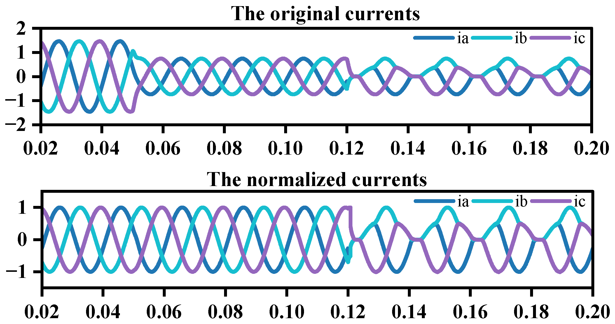
As shown in Figure 5, the three original phase currents are simultaneously affected by operating-condition variation and the ${\mathrm{S}}_3$ SCF, resulting in evident changes in both the overall amplitude and the interphase relationship. After the proposed normalization strategy is applied, the amplitude variation caused by operating-condition changes is effectively suppressed, while the structural abnormality associated with the ${\mathrm{S}}_3$ SCF is preserved, thus providing a more consistent input for subsequent fault-feature extraction.

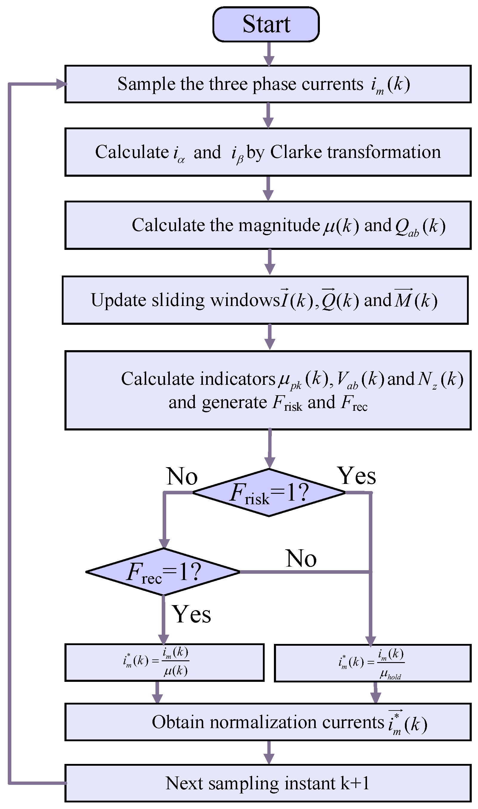
The normalization flowchart is shown in Figure 6. On the basis of the extracted magnitude and local structural information, the proposed method generates the risk and recovery conditions and then adaptively switches between the instantaneous normalization mode and the held-value normalization mode.

3.3. Fault Diagnosis Method

The fault detection and localization method is adopted: first, determine the theoretical operating sector by identifying the phase with the largest current and its polarity; then, calculate the variation trends in the same-polarity currents.

Define $P_m$ as the polarity variable.

$${\mathrm{P}}_{\mathrm{m}}\left(k\right)=\left\{\begin{array}{cc}1& i_m^{*}\left(k\right)>{\epsilon }_1\hfill \\ -1& i_m^{*}\left(k\right)<-{\epsilon }_1\hfill \\ {\mathrm{P}}_{\mathrm{m}}(k-1)& |i_m^{*}\left(k\right)|<{\epsilon }_1\hfill \end{array}\right.$$

(35)

where ${\epsilon }_1$ is a threshold is used to reduce noise interference when one phase current approaches zero. When all three phase currents are less than ${\epsilon }_1$, $P_a=P_b=P_c=0$.

$$S\left(k\right)=\left\{\begin{array}{cc}1\hfill & (P_a,P_b,P_c)=(1,-1,-1)\hfill \\ 2\hfill & (P_a,P_b,P_c)=(1,1,-1)\hfill \\ 3\hfill & (P_a,P_b,P_c)=(-1,1,-1)\hfill \\ 4\hfill & (P_a,P_b,P_c)=(-1,1,1)\hfill \\ 5\hfill & (P_a,P_b,P_c)=(-1,-1,1)\hfill \\ 6\hfill & (P_a,P_b,P_c)=(1,-1,1)\hfill \\ 0\hfill & (P_a,P_b,P_c)=(0,0,0)\hfill \end{array}\right.$$

(36)

When normalization is complete, the amplitude scale of the three phase currents has been unified, which facilitates subsequent construction of discrete trend features. To extract the phase-current variation trend, the normalized phase-current signals are staircase-quantized, and a memory-based trend variable is further defined.

The interval $[0°,90°]$ is equally divided into 18 segments, and the corresponding angular resolution is

$$\Delta \theta ={\displaystyle \frac{90°}{18}}=5°.$$

(37)

Accordingly, the staircase index signal of the phase current is defined as

$$S_m\left(k\right)=\left\{\begin{array}{cc}n,\hfill & \sin \left((n-1)\Delta \theta \right)\le i_m^{*}\left(k\right)<\sin \left(n\Delta \theta \right),\hfill \\ -n,\hfill & \sin \left((n-1)\Delta \theta \right)<-i_m^{*}\left(k\right)\le \sin \left(n\Delta \theta \right).\hfill \end{array}\right.$$

(38)

As shown in (38), the normalized phase current is quantized into 18 symmetric staircase intervals on the positive and negative half-axes, respectively, so that the continuous phase-current signal is converted into a discrete staircase representation.

To suppress fluctuations near staircase boundaries, a staircase confirmation mechanism is introduced. Let $S_x\left(k\right)$ denote the original staircase signal from (38), and let ${\overline{S}}_x\left(k\right)$ denote the effective staircase signal for trend extraction. The latter is updated only when the new staircase value persists for three consecutive samples. Thus, ${\overline{S}}_x\left(k\right)$ is defined as

$$\Delta {\overline{S}}_m\left(k\right)={\overline{S}}_m\left(k\right)-{\overline{S}}_m(k-1),m\in \{a,b,c\}.$$

(39)

Since two adjacent samples may fall into the same staircase interval, $\Delta S_x\left(k\right)=0$ does not necessarily imply that the actual trend has vanished; rather, it usually indicates that the signal has not crossed the neighboring staircase boundary at the current sampling instant. To avoid frequent resets of the trend signal caused by quantization, a memory-based trend definition is adopted.

$$d_m\left(k\right)=\left\{\begin{array}{cc}0,\hfill & S\left(t\right)=0,\hfill \\ \Delta {\overline{S}}_m\left(k\right),\hfill & S\left(k\right)\ne 0\mathrm{and}\Delta {\overline{S}}_m\left(k\right)\ne 0,\hfill \\ d_m(k-1),\hfill & S\left(k\right)\ne 0\mathrm{and}\Delta {\overline{S}}_m\left(k\right)=0.\hfill \end{array}\right.$$

(40)

In (40), the zero trend appears only when all three phase currents simultaneously remain in the zero-current state; when the staircase difference is zero, the trend variable keeps its previous value.

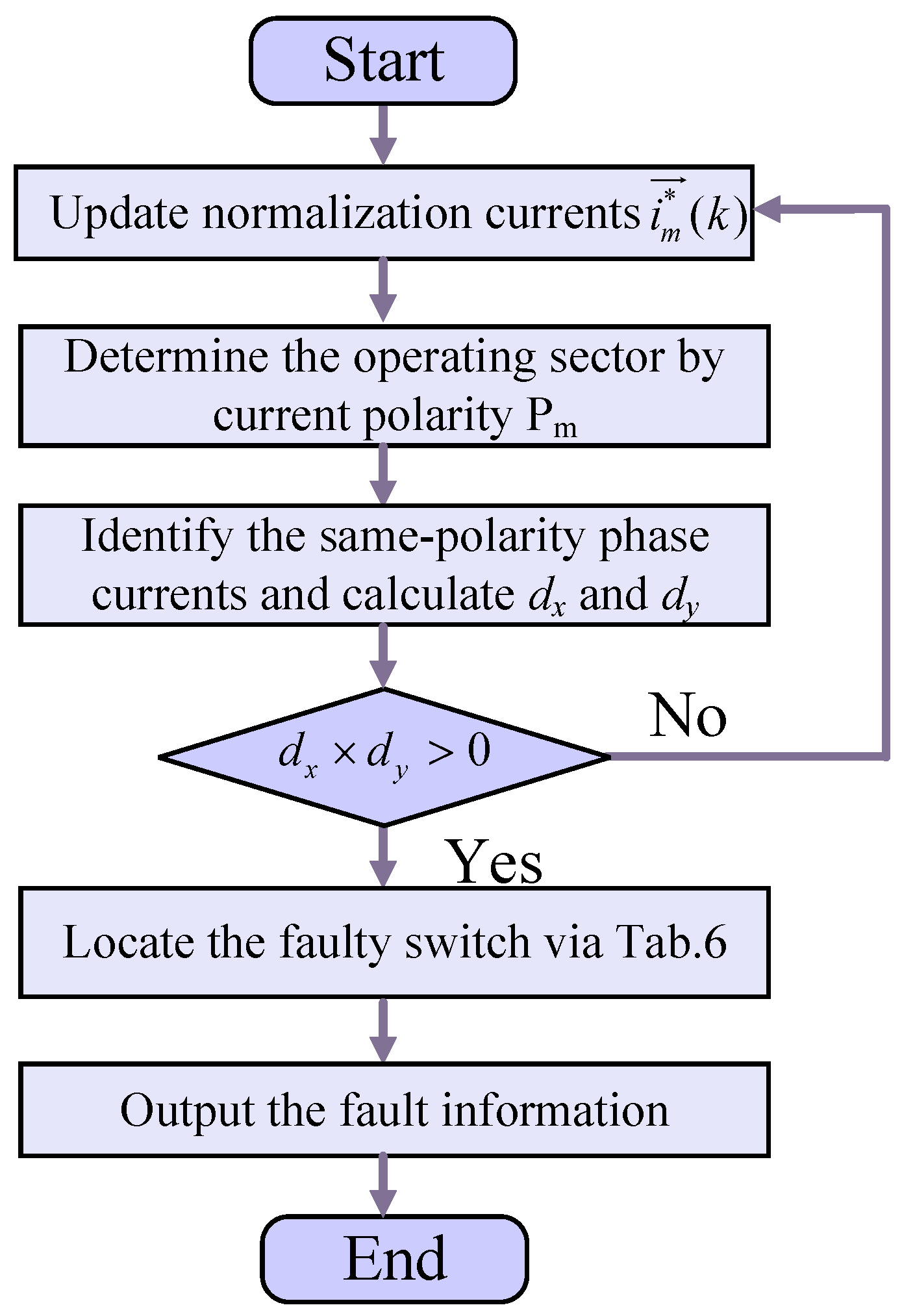
In the sector where two phase currents have the same polarity, let $d_x$ and $d_y$ denote the corresponding current-trend quantities. When their product satisfies $d_x{d}_y>0$, the two same-polarity currents are considered to exhibit the same variation trend, indicating the presence of a short-circuit fault feature. Then, by combining the current operating sector with the sign information of $d_x$ and $d_y$, the faulty switch can be further identified. The corresponding fault-location table is given in

Table 6. Fault location table for SCFs in a CSI.

Faulty Switch	Sector Output	${\mathit{d}}_{\mathit{a}}$	${\mathit{d}}_{\mathit{b}}$	${\mathit{d}}_{\mathit{c}}$
S1 SCF	2	<0	<0
	6	>0		>0
S2 SCF	1	<0	<0
	3	>0		>0
S3 SCF	2	>0	>0
	4		<0	<0
S4 SCF	3	<0		<0
	5	>0	>0
S5 SCF	4		>0	>0
	6	<0		<0
S6 SCF	1		>0	>0
	5	<0	<0

.

On the basis of the preceding analysis, Figure 7 provides a flowchart of the proposed fault diagnosis method.

Single-switch SCF features form the basis for multi-switch fault localization. A single-switch fault produces the same feature in two associated sectors; for example, an ${\mathrm{S}}_1$ short-circuit yields identical ${\mathrm{S}}_1$-related features in Sectors II and IV. In contrast, a multi-switch fault appears as a combination of single-switch fault features. Hence, the simultaneous detection of one ${\mathrm{S}}_1$-related feature and one ${\mathrm{S}}_2$-related feature indicates an ${\mathrm{S}}_1$ and ${\mathrm{S}}_2$ SCF.

4. Analysis of Experimental Results

4.1. Experimental Waveform Analysis

The experimental results confirm the effectiveness of the proposed method. The relevant parameters of the experiment are shown in

Table 7. Parameters of the experimental platform.

Parameter	Name	Value
$U_{\mathrm{dc}}$	Buck input voltage	40 V
$I_{\mathrm{dc}}$	Buck output current	3 A
$L_{\mathrm{dc}}$	DC-side inductor	5 mH
$C_{\mathrm{m}}$	Filter capacitor	9.4 $\mathrm{\mu }\mathrm{F}$
$R_{\mathrm{load}}$	Load resistance	20 $\Omega$
$L_{\mathrm{load}}$	Load inductor	2.5 mH
$\gamma$	Magnitude-depth threshold	0.9
$\sigma$	Variation-rate threshold	0.1
$\eta$	Unified structural threshold	0.05
${\epsilon }_1$	Near-zero threshold	0.1
N	Total number of samples in sliding window	15
$L_p$	Number of samples used for decision	5

.

The threshold values reported in this paper, $\gamma =0.9$, $\sigma =0.1$, $\eta =0.05$…, were selected on the basis of the specific experimental platform. For general application to other current-source inverters, these parameters may need to be recalibrated. Specifically, $\gamma$ and $\sigma$ can be tuned during commissioning under rapid magnitude-variation conditions, while ${\epsilon }_1$ and $\eta$ should be adjusted according to the noise and ripple levels of the current measurements to ensure reliable polarity and sector determination.

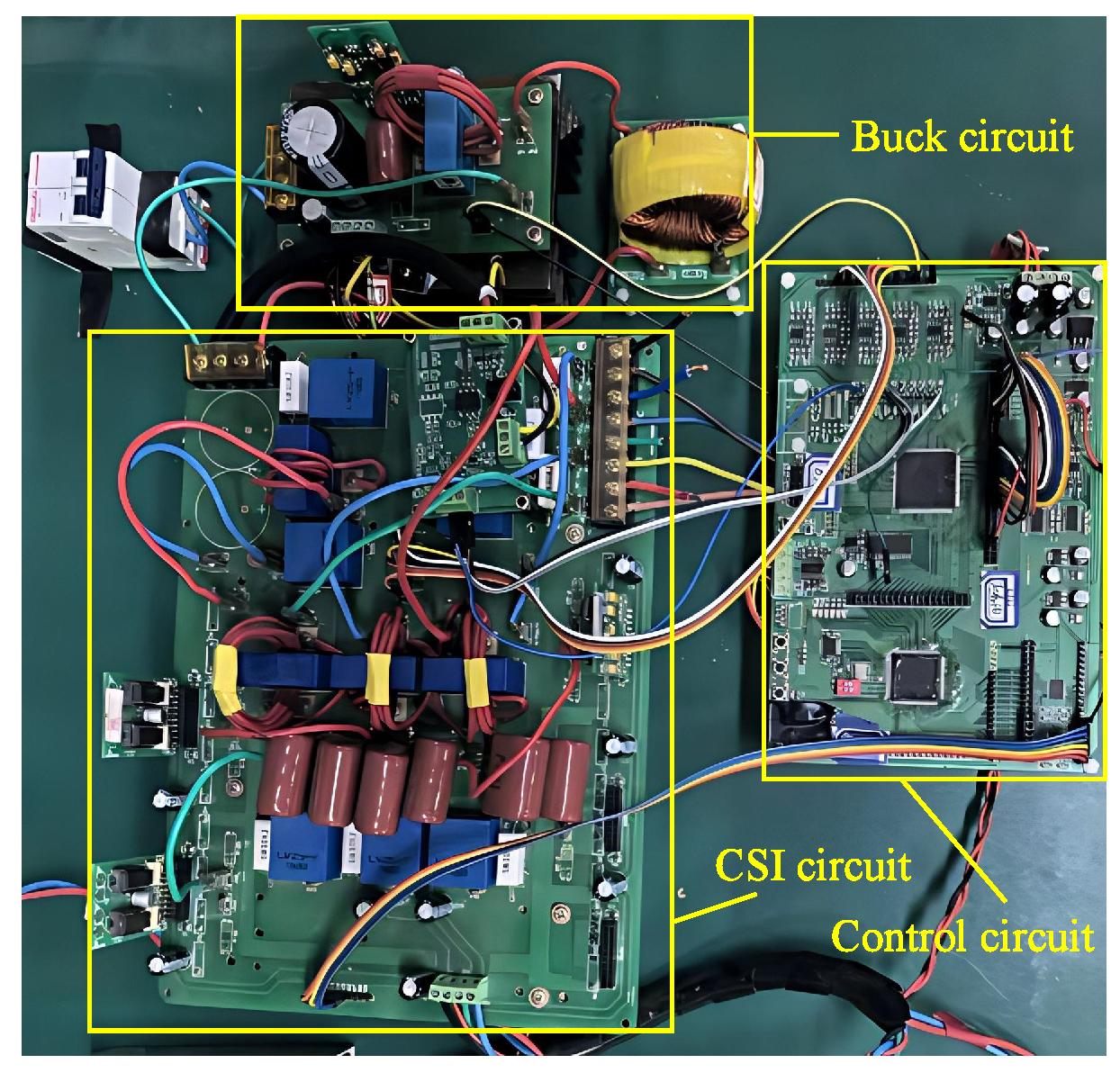
Figure 8 illustrates the experimental setup. A buck converter is employed to generate the input current, while the output current is generated by the CSI on the basis of the SVPWM scheme. The control system is implemented using a DSP (TMS320F28335) and an FPGA (XC6SLX92TQG144C), and the detection results are output via the DSP D/A port.

4.1.1. Diagnosis Results for Single-Switch Faults

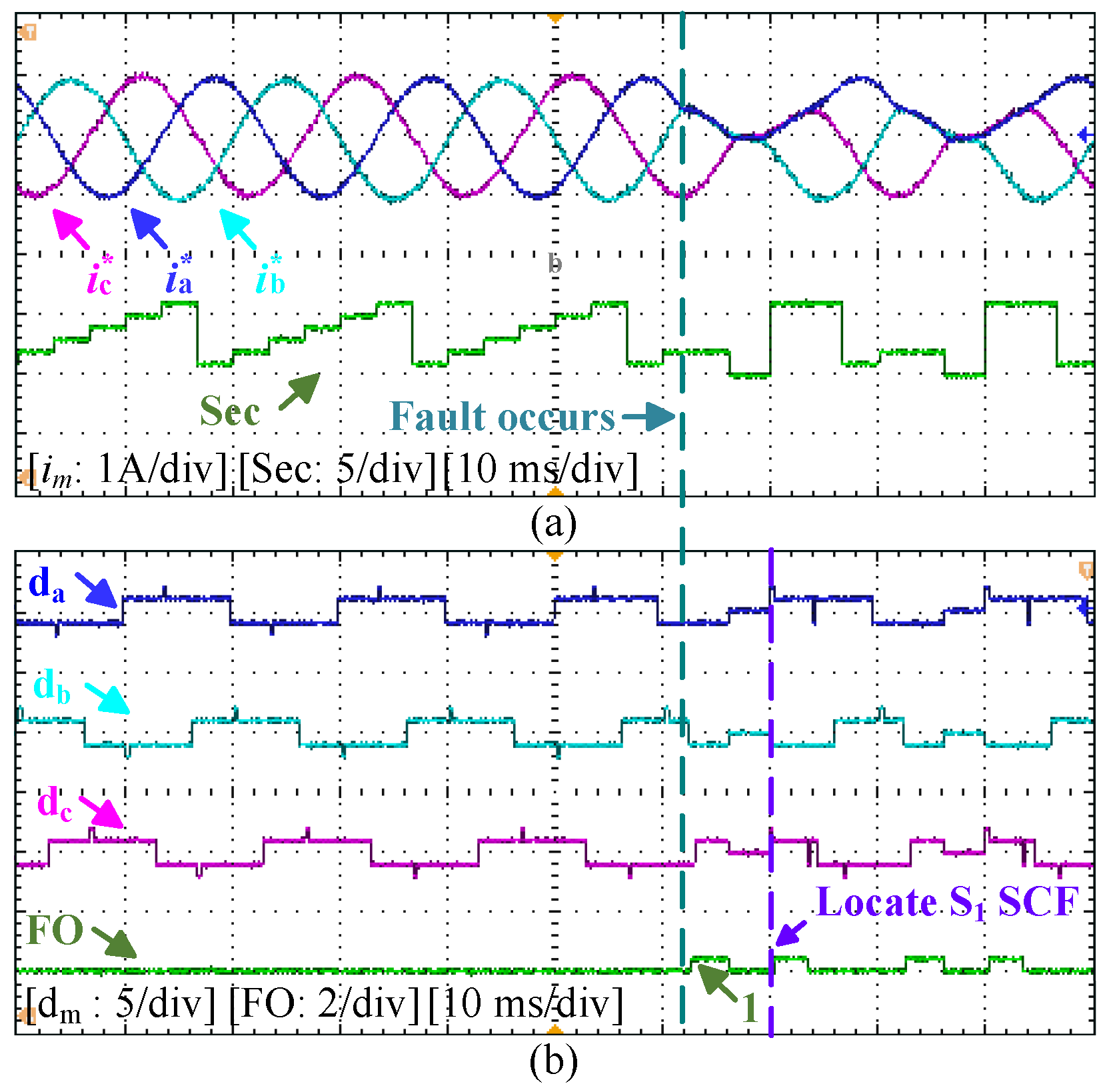
As shown in Figure 9a, when an ${\mathrm{S}}_1$ short-circuit fault occurs, the three phase currents and the corresponding sector signal $S\left(t\right)$ change accordingly after the instant of the fault. As shown in Figure 9b, the proposed method further extracts the current-trend signals $d_a$, $d_b$, and $d_c$, and generates the fault output $FO$. According to the sector information and the polarity of the same-polarity current-trend signals, the fault is successfully localized as an ${\mathrm{S}}_1$ SCF.

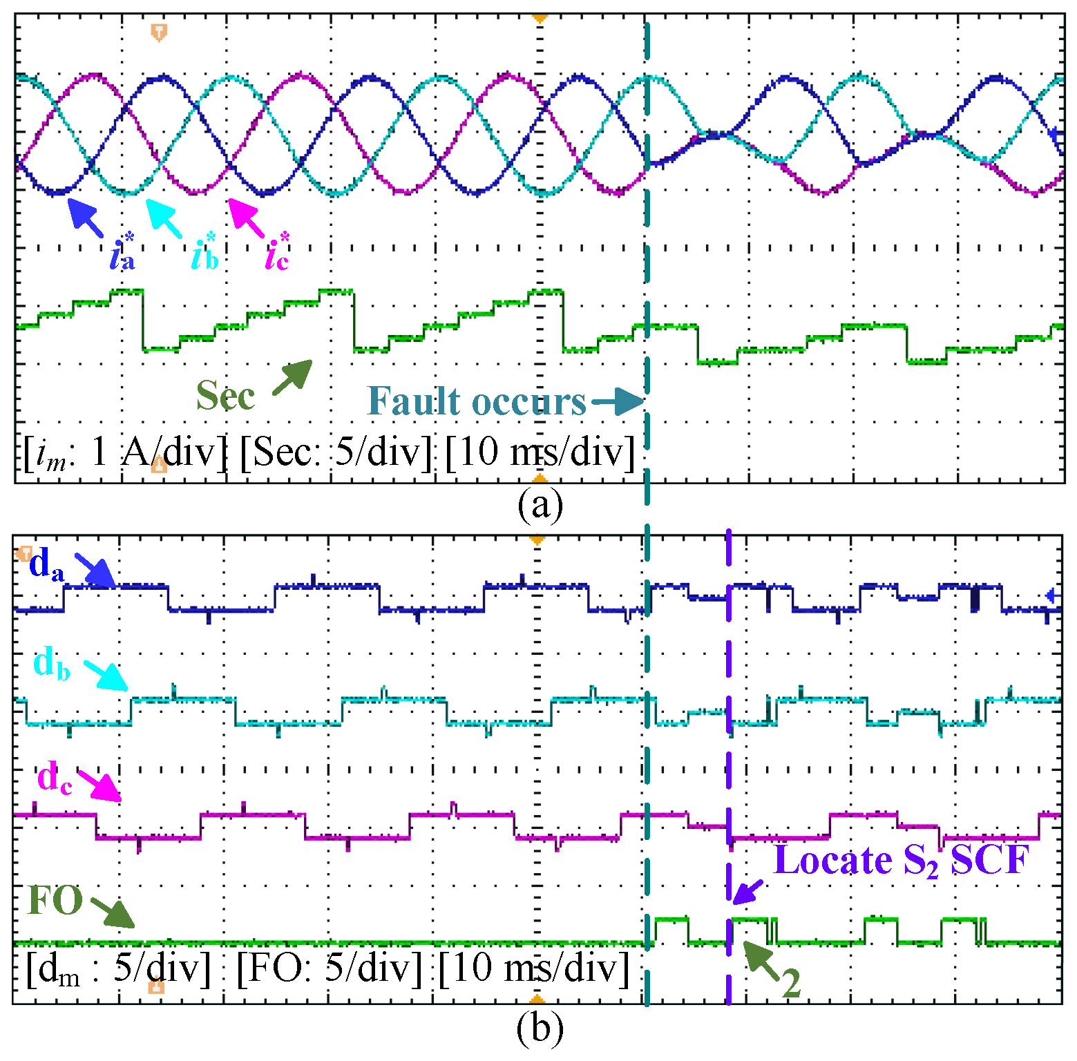
Figure 10 illustrates the waveform response under an ${\mathrm{S}}_2$ SCF. In Figure 10a, the three phase currents together with the sector signal $S\left(t\right)$ are shown, where the fault occurs at the marked instant. After the fault is introduced, the current waveforms exhibit evident structural variation. In Figure 10b, the corresponding current-trend signals $d_a$, $d_b$, and $d_c$ are obtained, and the fault output $FO$ is generated accordingly. On the basis of the operating sector and the sign combination of the same-polarity current-trend signals, the proposed method correctly identifies the faulty switch as ${\mathrm{S}}_2$.

4.1.2. Multi-Switch Fault Diagnosis Test

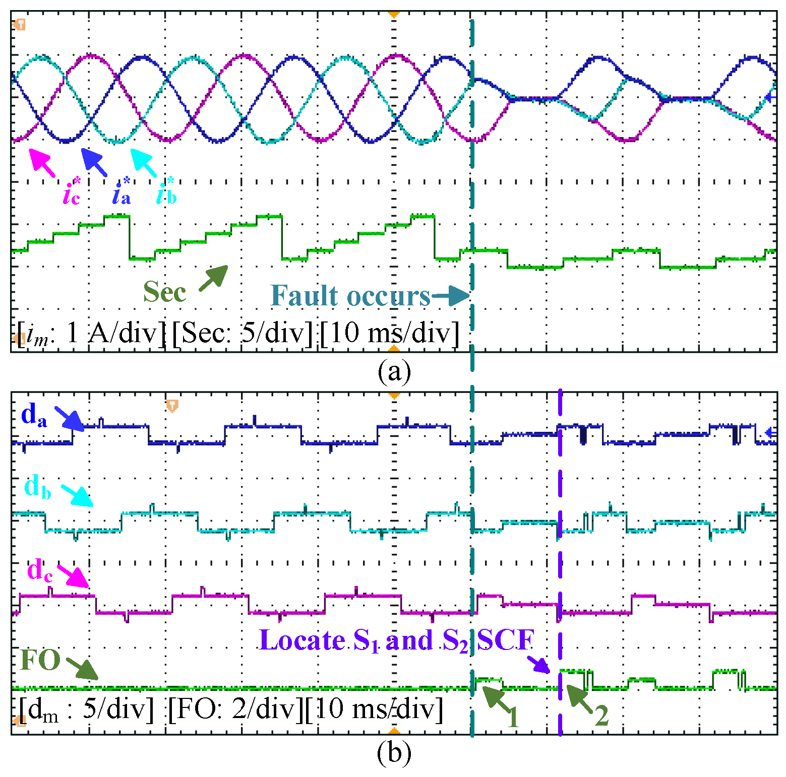
Figure 11 shows the diagnosis result for a simultaneous short-circuit fault of S1 and S2. As shown in Figure 11a, after the marked instant of the fault, the three phase currents and the corresponding sector signal $S\left(t\right)$ exhibit evident abnormal changes. As shown in Figure 11b, the proposed method further extracts the current-trend signals $d_a$, $d_b$, and $d_c$ and generates the fault output $FO$.

EAfter the fault occurs, two distinct fault features are first extracted by combining the operating sector information with the sign combination of the same-polarity current-trend signals. Then, according to the correspondence between these two extracted features and the single-switch short-circuit fault signatures, they are identified as the fault features of S1 and S2, respectively. Therefore, the proposed method can accurately diagnose a simultaneous SCF of ${\mathrm{S}}_1$ and ${\mathrm{S}}_2$.

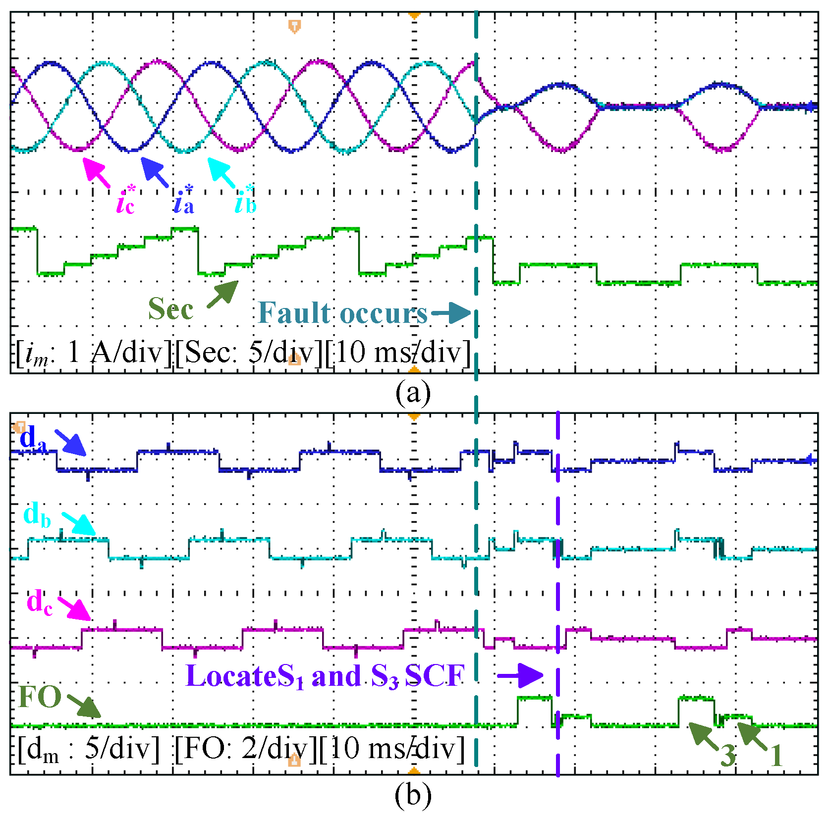
Figure 12 presents the diagnosis result for a simultaneous short-circuit fault of S1 and S3. As shown in Figure 12a, once the fault is introduced at the marked instant, the three phase currents and the corresponding sector signal $S_i\left(t\right)$ exhibit noticeable abnormal variations. In Figure 12b, the proposed method extracts the current-trend signals $d_a$, $d_b$, and $d_c$ and generates the fault output $FO$. By combining the operating sector information with the sign pattern of the same-polarity current-trend signals, two fault features are identified after the fault occurrence. By their correspondence to the single-switch short-circuit fault signatures, these two features are further recognized as the fault characteristics of S1 and S3, respectively. Hence, the proposed method successfully diagnoses a simultaneous short-circuit fault of S1 and S3.

4.1.3. Dynamic Performance Testing

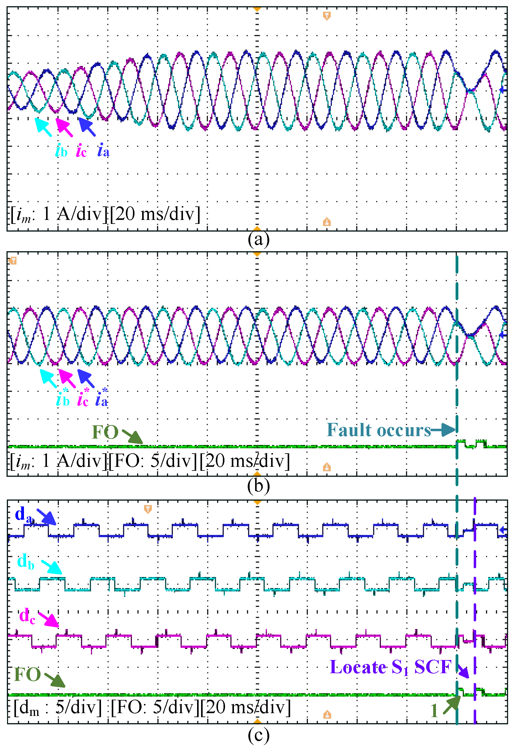
Figure 13 presents the results of online detection and location of the S1 SCF under variable-load conditions. During the load variation, the amplitudes of the three phase currents change noticeably, while their normal phase relationship and periodic structure are still preserved; therefore, no false response appears in $FO$. After the fault occurs at the marked instant, both the current waveforms and the trend signals $d_a$, $d_b$, and $d_c$ exhibit clear abnormal features, and $FO$ responds accordingly. By combining the operating sector information with the sign relationship of the same-polarity current-trend signals, the proposed method can effectively distinguish the fault from load variation and accurately identify ${\mathrm{S}}_1$ as the faulty switch.

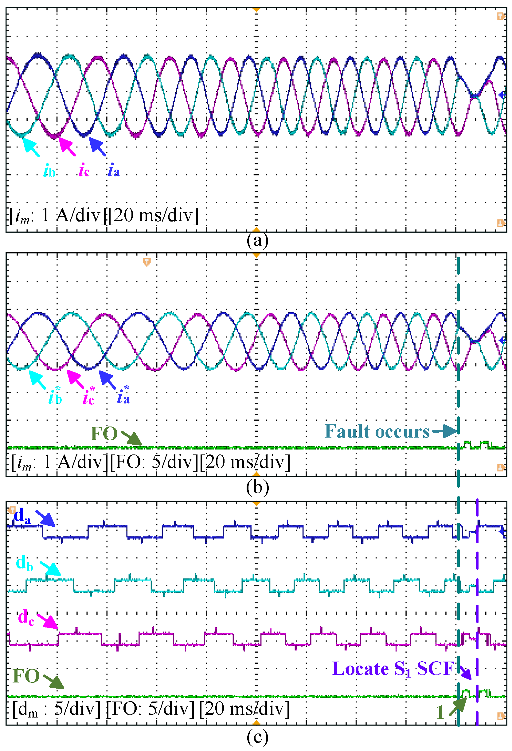
As shown in Figure 14a, the operating frequency of the inverter continuously varies between 25 Hz and 50 Hz, and the amplitude of the original three phase currents changes dynamically. In Figure 14b, the proposed normalization method outputs normalized currents with constant amplitude while preserving the frequency variation characteristics. In Figure 14c, the variation trends of the three phase currents also change with frequency. Nevertheless, the proposed fault localization method can still accurately and quickly locate the faulty switch.

The experimental results indicate that the observed output currents and diagnostic results are consistent with the theoretical analysis in Section 3 and Table 6. Thus, the effectiveness of the proposed method is experimentally confirmed.

4.2. Comparison with Other Methods

Compared with conventional current normalization methods (e.g., fixed-window peak or RMS normalization), the proposed method adaptively distinguishes normal load-induced amplitude variations from fault-induced structural abnormalities by evaluating risk conditions (magnitude depth, fixed-ratio structure, and near-zero collapse). It switches between instantaneous normalization and held-value normalization, thereby preserving fault-induced relative changes while suppressing load-driven fluctuations.

To further evaluate the performance of the proposed algorithm, the comparative results were tabulated, as presented in

Table 8. Performance comparison of different fault diagnosis methods.

Relevant Method	Additional Circuit	Load Variation	Frequency Variation	Multi-Tube Faults	Diagnosis Principle	Localization Time
[17]	Yes	Yes	Yes	No	Capacitor voltage	<$0.25T_{\mathrm{base}}$
[22]	No	Yes	No	Yes	Current ratio	≈$1.25T_{\mathrm{base}}$
[23]	No	Yes	Yes	Yes	Current phase angle	≈$T_{\mathrm{base}}$
Proposed method	No	Yes	Yes	Yes	Current trend	≈$0.75T_{\mathrm{base}}$

and

Table 9. Summary of experimental cases and diagnostic results.

Fault Case	Load Condition	Frequency (Hz)	Localization Time (ms)	Correct Diagnosis
S1 SCF	R-L	50	9	Yes
S2 SCF	R-L	50	10	Yes
S1 and S2 SCF	R-L	50	11	Yes
S1 and S3 SCF	R-L	50	12	Yes
S1 SCF	R-L ($0.6$ → 1.5 A)	50	10	Yes
S1 SCF	R-L	25→50	12	Yes

.

Table 8 compares the proposed method with existing CSI switch short-circuit fault diagnosis methods. In contrast to [17], the proposed method requires no additional sampling circuit and is applicable to multiple-switch faults. Compared with [22], it further considers frequency variation and reduces the localization time to approximately $0.75T_{\mathrm{base}}$. Compared with [23], the proposed method retains the advantages of no additional sampling circuit, adaptability to load and frequency variations, and applicability to multiple-switch faults, while achieving an average localization time of approximately $0.75T_{\mathrm{base}}$. Thus, the proposed method is 25–50% faster than [22] and 15–20% faster than [23] while retaining the same advantage of requiring no additional circuits.

Therefore, the proposed method provides a good balance among hardware simplicity, operating-condition adaptability, fault coverage, and localization speed.

5. Conclusions

In this paper, a fault-locating method based on the polarity and variation trends in normalized phase currents is proposed. The method is derived from the circuit topology constraints of CSIs in general. It is shown that, after an SCF occurs, the variation trends in the two same-polarity phase currents exhibit consistent sign characteristics in specific operating sectors. On the basis of this fault feature, the proposed diagnosis method has good interpretability. The method requires no additional sampling circuit, and thus has low implementation cost. For multi-switch SCFs, it also provides a faster diagnostic response than conventional methods. Experimental results demonstrate that the proposed method can accurately locate the faulty switch. Moreover, it maintains high robustness under operating conditions with continuously varying output-current magnitude and frequency. Therefore, the proposed method has good potential for practical engineering applications.

6. Discussion

A limitation of the proposed method is observed under single-phase overload conditions. In such cases, one phase current becomes significantly smaller than the other two. As a result, the normalized current of that phase changes slowly, which may reduce the accuracy of the relative variation trend estimation and potentially delay fault diagnosis. Addressing this limitation will be a focus of our future work. Moreover, it should be acknowledged that the present experiments, despite showing the robustness of the method under load/frequency variations, have not addressed more severe non-ideal conditions (e.g., extreme noise or sensor offsets). Such realistic hardware validation is left for future work.

References

1. Teng, Y.; Wei, Y.; Li, Y.; Guo, X.; Li, Y. An Overview of Current Source Converters: State-of-the-Art and Future Trends. IEEE Trans. Power Electron. 2026, 41, 9959–9984. [Google Scholar]
2. Yang, S.; Yin, Z.; Tong, C.; Sui, Y.; Zheng, P. Active Damping Current Control for Current-Source Inverter-Based PMSM Drives. IEEE Trans. Ind. Electron. 2023, 70, 3549–3560. [Google Scholar]
3. Gundogmus, O.; Harasis, S.; Chowdhury, S.M.; Vadamodala, L.; Das, S.; Haque, E.; Sozer, Y.; Venegas, F.; Colavincenzo, D. Comparison of failure modes, effect analysis and reliability of electric machine drives. In 2019 IEEE International Electric Machines & Drives Conference (IEMDC); IEEE: Piscataway, NJ, USA, 2019; pp. 916–921. [Google Scholar]
4. Xing, L.; Wei, Q.; Li, Y. A PWM Current-Source Converter-Based Wind Energy Conversion System. IEEE Trans. Power Electron. 2024, 39, 2787–2797. [Google Scholar] [CrossRef]
5. Xing, L.; Wei, Q.; Li, R. An Improved Current-Source-Converter-Based Series-Connected Wind Energy Conversion System. IEEE Trans. Ind. Electron. 2024, 71, 4818–4829. [Google Scholar] [CrossRef]
6. Xia, Y.; Xu, Y. A Robust Data-Driven Method for Open-Circuit Fault Diagnosis of Power Switches in Three-Phase Inverters With Low-Quality Data. IEEE Trans. Power Electron. 2025, 40, 5949–5958. [Google Scholar]
7. Wu, R.; Blaabjerg, F.; Wang, H.; Liserre, M.; Iannuzzo, F. Catastrophic Failure and Fault-Tolerant Design of IGBT Power Electronic Converters—An Overview. In Proceedings of the IECON 2013—39th Annual Conference of the IEEE Industrial Electronics Society, Vienna, Austria, 10–13 November 2013; IEEE: Piscataway, NJ, USA, 2013; pp. 507–513. [Google Scholar]
8. Ajra, Y.; Hoblos, G.; Al Sheikh, H.; Moubayed, N. A Literature Review of Fault Detection and Diagnostic Methods in Three-Phase Voltage-Source Inverters. Machines 2024, 12, 631. [Google Scholar] [CrossRef]
9. Lee, S.; Chen, F.; Jahns, T.M.; Sarlioglu, B. Topological Equivalence of VSI and CSI Commutation Cells and Its Application to Switching Resonance Analysis and Damper Design. IEEE Trans. Transp. Electrif. 2024, 10, 1363–1376. [Google Scholar] [CrossRef]
10. Song, W.; Xu, P.; Chen, J.; Tan, H.; Yang, K.; Tang, T. A Chip Open-Circuit Failure Monitoring Method in Multichip IGBT Modules Based on the Fall Time of Gate Voltage. IEEE Trans. Transp. Electrif. 2024, 10, 8224–8234. [Google Scholar] [CrossRef]
11. Yu, S.; Wang, Z.; Tan, L.; Qin, J.; Zhou, D.; Wu, Y.; Zhou, Y.; Xin, G.; Shi, X. A Gate Open-Circuit Failure Detection Method of SiC MOSFETs Based on Internal Gate State Extraction. IEEE Trans. Power Electron. 2024, 39, 16638–16650. [Google Scholar] [CrossRef]
12. Ouyang, W.; Sun, P.; Xie, M.; Luo, Q.; Du, X. A Fast Short-Circuit Protection Method for SiC MOSFET Based on Indirect Power Dissipation Level. IEEE Trans. Power Electron. 2022, 37, 8825–8829. [Google Scholar] [CrossRef]
13. Lei, X.; Wu, F.; Liu, Y. An Online Convolutional Neural Network Based Method for Open-Circuit Fault Diagnosis in Three-Phase Inverters Under Extremely Unbalanced Loading Condition. IEEE Trans. Power Electron. 2026, 1–14. [Google Scholar] [CrossRef]
14. Sun, X.; Diao, N.; Song, C.; Qiu, Y.; Zhao, X. An Open-Circuit Fault Diagnosis Method Based on Adjacent Trend Line Relationship of Current Vector Trajectory for Motor Drive Inverter. Machines 2023, 11, 928. [Google Scholar] [CrossRef]
15. Shu, C.; Chen, Y.-T.; Yang, T.-J.; Wang, X. A Novel Diagnostic Technique for Open-Circuited Faults of Inverters Based on Output Line-to-Line Voltage Model. IEEE Trans. Ind. Electron. 2016, 63, 4412–4421. [Google Scholar] [CrossRef]
16. Sun, X.; Song, C.; Zhang, Y.; Sha, X.; Diao, N. An Open-Circuit Fault Diagnosis Algorithm Based on Signal Normalization Preprocessing for Motor Drive Inverter. IEEE Trans. Instrum. Meas. 2023, 72, 3513712. [Google Scholar] [CrossRef]
17. Chen, B.; Sun, Y.; Xie, S.; Liu, Y.; Dan, H.; Yu, B.; Su, M. A Hybrid Short-Circuit Fault Diagnosis Method for Current Source Inverters. IEEE Trans. Ind. Electron. 2026, 73, 3426–3436. [Google Scholar] [CrossRef]
18. Zhang, X.; Gauthier, J.-Y.; Lin-Shi, X. Cost-Efficient Fault-Tolerant Scheme for Three-Phase Surface-Mounted Permanent Magnet Synchronous Machines Fed by Multifunctional Converter System Under Open-Phase Faults. IEEE Trans. Ind. Electron. 2022, 69, 5502–5513. [Google Scholar] [CrossRef]
19. Huang, Z.; Wang, Z.; Zhang, H. A Diagnosis Algorithm for Multiple Open-Circuited Faults of Microgrid Inverters Based on Main Fault Component Analysis. IEEE Trans. Energy Convers. 2018, 33, 925–937. [Google Scholar] [CrossRef]
20. Luo, Y.; Zhang, L.; Chen, C.; Li, K.; Li, K. Real-Time Diagnosis of Open Circuit Faults in Three-Phase Voltage Source Inverters. IEEE Trans. Power Electron. 2024, 39, 7572–7585. [Google Scholar] [CrossRef]
21. Zhang, Y.; Liu, Y.; Kang, S.; Wang, P. Current Vector Phase Based Weak Open-Circuit Fault Diagnosis of Voltage-Source Inverters. IEEE Trans. Power Electron. 2026, 41, 9502–9512. [Google Scholar] [CrossRef]
22. Guo, X.; Sui, S.; Wang, B.; Zhang, W. A Current-Based Approach for Short-Circuit Fault Diagnosis in Closed-Loop Current Source Inverter. IEEE Trans. Ind. Electron. 2020, 67, 7941–7950. [Google Scholar] [CrossRef]
23. Teng, Y.; Guo, X.; Wei, Y.; Zhao, J.; Zhang, P. A Novel Short-Circuit Fault Diagnosis Method for Three-Phase Current Source Converter. IEEE Trans. Power Electron. 2024, 39, 16792–16802. [Google Scholar]
Figure 1. The typical topology of a three-phase CSI.
Machines 14 00710 g001
Figure 2. Space vector diagram of a CSI.
Machines 14 00710 g002
Figure 3. Correspondence between active vector conduction times and inverter operating conditions.
Machines 14 00710 g003
Figure 4. Actual current flow diagram when an SCF occurs in S 3 .
Machines 14 00710 g004
Figure 5. Comparison between the original and normalized current waveform diagrams.
Machines 14 00710 g005
Figure 6. Flowchart of the proposed normalization method.
Machines 14 00710 g006
Figure 7. Flowchart of the proposed fault diagnosis and localization method.
Machines 14 00710 g007
Figure 8. Experimental platform.
Machines 14 00710 g008
Figure 9. Experimental results for an SCF occurring in S 1 . (a) Waveforms of the three normalized phase current signals and Sec. (b) Three-phase current variation trends and fault result output.
Machines 14 00710 g009
Figure 10. Experimental results for an SCF occurring in S 2 . (a) Waveforms of the three normalized phase current signals and Sec. (b) Three-phase current variation trends and fault result output.
Machines 14 00710 g010
Figure 11. Experimental results for an SCF occurring in S 1 and S 2 . (a) Waveforms of the three normalized phase current signals and Sec. (b) Three-phase current variation trends and fault result output.
Machines 14 00710 g011
Figure 12. Experimental results for an SCF occurring in S 1 and S 3 . (a) Waveforms of the three normalized phase current signals and Sec. (b) Three-phase current variation trends and fault result output.
Machines 14 00710 g012
Figure 13. Experimental results of an S 1 SCF under variable-frequency conditions. (a) Waveforms of the three original phase current signals. (b) Waveforms of the three normalized phase current signals and fault result output. (c) Three-phase current variation trend and fault result output.
Machines 14 00710 g013
Figure 14. Experimental results of an S 1 SCF under variable-load conditions. (a) Waveforms of the three original phase current signals. (b) Waveforms of the three normalized phase current signals and fault result output. (c) Three-phase current variation trend and fault result output.
Machines 14 00710 g014