Article

A Multi-Class Predictive Maintenance Framework for Jet Engines Using the C-MAPSS Dataset

1
School of Electrical Automation and Information Engineering, Tianjin University, Tianjin 300072, China
2
Department of Computer Science, Rochester Institute of Technology, Rochester, NY 14623, USA
3
Department of Computer Science, Rutgers University, New Brunswick, NJ 08901, USA
4
Department of Computer Science and Engineering, Santa Clara University, Santa Clara, CA 95053, USA
5
Meta Platforms Inc., Menlo Park, CA 94025, USA
6
Graduate School of Arts and Science, Yale University, New Haven, CT 06520, USA
*
Author to whom correspondence should be addressed.
Machines 2026, 14(6), 695; https://doi.org/10.3390/machines14060695
Submission received: 6 May 2026 / Revised: 7 June 2026 / Accepted: 15 June 2026 / Published: 17 June 2026

Abstract

Aero-engine predictive maintenance is challenged by heterogeneous operating conditions, complex degradation patterns, and the need for interpretable maintenance alerts rather than solely numerical life estimates. This study investigates a condition-aware data-driven framework for jet engine health assessment using the NASA C-MAPSS dataset, which contains four benchmark subsets (FD001–FD004) with different operating conditions and fault modes. Instead of formulating the task as conventional remaining useful life regression, this study reformulates degradation assessment as a three-class health state classification problem, including Normal, Warning, and Fault. A unified preprocessing pipeline is developed, incorporating condition-wise normalization, first-order differential feature construction, and per-unit sliding window segmentation to reduce operating-condition bias, capture degradation dynamics, and prevent data leakage. Five representative models are evaluated under the same framework, including XGBoost, LightGBM, Random Forest, a context-aware multi-scale temporal attention convolutional neural network, and a bidirectional long short-term memory network. The results show that the proposed framework achieves consistently high classification accuracy across all four subsets, with the best results of 0.9841 on FD001, 0.9764 on FD002, 0.9891 on FD003, and 0.9832 on FD004. In addition, Bi-LSTM outperforms MSTA-CNN on all subsets, for example improving accuracy from 0.9614 to 0.9747 on FD002 and from 0.9773 to 0.9806 on FD004, which is consistent with the importance of long-term temporal dependency modeling for this task. These findings suggest that the proposed framework provides an effective and maintenance-decision-aligned solution for C-MAPSS-based health monitoring, where the three-class alert output offers clearer operational meaning than a single numerical life estimate.

1. Introduction

1.1. Research Background and Motivation

Aero-engines are safety-critical and high-value systems whose operational reliability directly affects flight safety, maintenance cost, and fleet availability [1]. In practical engineering applications, conventional maintenance strategies are mainly based on fixed schedules or post-failure repair. Such strategies often result in either excessive maintenance or delayed intervention, making them increasingly unsuitable for modern aviation systems with high requirements for reliability, economy, and operational continuity [2]. Under this background, predictive maintenance has become an important research direction in aero-engine health management because it enables maintenance decisions to be supported by condition monitoring, degradation assessment, and data-driven prediction.
The NASA C-MAPSS dataset has been widely adopted in aero-engine degradation analysis and prognostics research. It contains four subsets, FD001–FD004, with different operating conditions and fault modes, thereby providing a representative benchmark for evaluating degradation modeling methods under different levels of complexity. Compared with simpler settings involving a single operating condition or a single fault mode, more complex subsets impose greater challenges on feature extraction, temporal modeling, and generalization. Therefore, this dataset provides a useful basis for studying predictive maintenance methods for aero-engines.
Most existing studies based on C-MAPSS formulate the task as continuous remaining useful life prediction. Although numerical RUL estimation is valuable for degradation assessment, a purely regression-based output is not always the most practical form for real maintenance operations [3]. In many cases, maintenance personnel are more concerned with whether an engine is still operating normally, has entered an early warning state, or is approaching a fault-critical stage. Compared with a single numerical prediction, such state-oriented outputs are often easier to interpret and more directly connected to maintenance decisions. Therefore, reformulating degradation prediction as a maintenance-oriented health state classification problem is meaningful from both methodological and application perspectives.

1.2. Literature Gap and Problem Statement

This study focuses on predictive maintenance for jet engines using the NASA C-MAPSS dataset. Instead of treating the task as a conventional continuous RUL regression problem, this work reformulates engine degradation assessment as a multi-class health state classification problem. More specifically, the engine degradation process is mapped into three health states, namely Normal, Warning, and Fault, so that the model output can serve directly as a maintenance alert signal. In this way, the prediction result is expressed in a form that is more closely aligned with maintenance decision-making and operational intervention.
To support this task formulation, a structured data preparation pipeline is constructed. First, rather than applying global normalization to all samples, the operating space is divided into multiple operating regimes, and normalization is performed within each regime in order to reduce the bias caused by environmental and operating-condition variation. Second, first-order differential features are introduced to capture the rate of change in sensor signals so that the model can better characterize degradation trends instead of relying only on static measurements. Third, sliding windows with a fixed length are generated strictly within each engine unit, ensuring that temporal samples preserve engine-specific degradation continuity and avoid data leakage across different units. These design choices reflect the idea that the effectiveness of predictive maintenance depends not only on model structure, but also on whether the input representation is consistent with the physical and operational properties of the monitored system.
Based on this framework, the objectives of this study are threefold. The first objective is to establish a maintenance-oriented classification framework that can effectively identify Normal, Warning, and Fault states for jet engines under multiple operating conditions. The second objective is to investigate the influence of condition-aware preprocessing and degradation-sensitive feature construction on health state recognition performance, particularly in more complex subsets with multiple operating regimes and fault modes. The third objective is to compare representative machine learning and deep learning methods within a unified experimental setting, so as to determine which modeling strategies are more suitable for maintenance alert generation in aero-engine applications.

1.3. Main Contributions

The main contributions of this study are summarized as follows.
(1)
A maintenance-oriented task reformulation is proposed for the C-MAPSS benchmark, converting continuous RUL regression into a three-class health state classification problem whose output—Normal, Warning, and Fault—corresponds directly to operational intervention thresholds. This reformulation shifts the prediction target from numerical life estimation to actionable maintenance alert generation, a distinction that is not merely cosmetic but changes how data are prepared, how models are trained, and how results are evaluated.
(2)
A jointly designed, condition-aware data preparation pipeline is developed in which condition-wise normalization, first-order differential feature construction, and per-unit sliding window segmentation are combined into a single coherent workflow. Unlike approaches that adopt each preprocessing step in isolation, the proposed pipeline is designed so that the three components address complementary sources of bias—operating-condition shift, static measurement limitation, and cross-unit data leakage—within a unified representation strategy.
(3)
Systematic empirical evidence is provided showing that the proposed preprocessing pipeline creates a sufficiently discriminative structured feature space for ensemble tree-based models to consistently match or exceed the classification performance of more complex deep temporal architectures across all four C-MAPSS subsets. This finding offers a practically important insight: for maintenance-oriented health state classification, well-designed data representation can be as consequential as model selection.
(4)
A class-level error analysis based on confusion matrices and ROC curves identifies the Warning state as the principal and consistent source of misclassification across all benchmark subsets and operating conditions. This result quantifies the inherent difficulty of transitional degradation stage recognition and pinpoints it as a focused direction for future improvement, independent of which model family is used.

1.4. Organization of the Paper

The remainder of this paper is organized as follows.
Section 2 reviews related work on aero-engine predictive maintenance and C-MAPSS-based degradation modeling.
Section 3 presents the proposed methods, including data description, problem formulation, preprocessing, feature engineering, and model development.
Section 4 reports the experimental settings and comparative results on the FD001–FD004 subsets.
Section 5 concludes the paper and discusses the main findings, limitations, and future research directions.

2. Related Works

2.1. Aero-Engine Prognostics and Predictive Maintenance

Aero-engine prognostics and predictive maintenance have attracted sustained attention because aero-engines operate in highly demanding environments and require strict reliability assurance throughout their service life [4]. Unlike conventional maintenance strategies based on fixed schedules or post-failure repair, predictive maintenance emphasizes the use of historical and real-time operational data to assess health conditions, identify degradation trends, and support timely maintenance intervention [5]. In this context, prognostics and health management has become an important research direction for improving maintenance efficiency, reducing operational risk, and extending equipment availability.
For aero-engine systems, the core objective of predictive maintenance is to extract meaningful degradation information from multivariate monitoring signals and translate it into decision-support outputs. Existing studies have mainly focused on fault diagnosis, health index construction, degradation stage recognition, and remaining useful life prediction. Among these topics, remaining useful life estimation has become the dominant formulation because it provides a direct quantitative description of the degradation process [6]. However, in practical maintenance scenarios, decision makers are often more concerned with whether the system remains in a safe operating region, has entered a warning stage, or requires immediate maintenance attention. Therefore, maintenance-oriented health state identification has clear practical value, particularly when the target is to provide operationally structured alert signals rather than only numerical prognostic outputs.
Another important characteristic of aero-engine predictive maintenance is the strong coupling between degradation behavior and operating conditions [7]. Sensor measurements are affected not only by component health but also by load variation, environmental changes, and operating regimes. As a result, reliable maintenance-oriented modeling requires methods that can distinguish degradation-related information from condition-induced variation. This makes condition adaptation, temporal pattern extraction, and robust health representation central issues in aero-engine prognostics research.

2.2. C-MAPSS-Based Health Assessment and Degradation Modeling

The C-MAPSS dataset has become one of the most widely used benchmark datasets for aero-engine degradation analysis [8]. Its broad adoption is mainly due to three advantages. First, it provides multivariate time-series monitoring data for multiple engine units over their full degradation trajectories [9]. Second, it includes several subsets with different numbers of operating conditions and fault modes, making it possible to evaluate model performance under both relatively simple and more complex scenarios [10]. Third, its benchmark status allows direct comparison across different modeling strategies [11].
Most studies based on C-MAPSS formulate the task as continuous remaining useful life prediction [12]. Under this setting, a large number of methods have been proposed, including statistical learning methods, shallow machine learning models, deep neural networks, and hybrid architectures. Early studies typically relied on manually designed features combined with conventional regressors [13]. With the development of deep learning, convolutional neural networks, recurrent neural networks, and attention-based temporal architectures have gradually become mainstream because of their ability to learn representations directly from sequential sensor data. In particular, recurrent structures are often used to model long-term degradation dependency, while convolutional structures are adopted to capture local temporal patterns and cross-sensor interactions.
Despite these advances, several issues remain evident in existing C-MAPSS-based research. First, many studies primarily optimize numerical regression error, while the maintenance relevance of the output receives less attention [14]. Second, the influence of operating conditions is not always handled explicitly, even though condition heterogeneity can significantly affect feature distributions and model generalization [15]. Third, many deep learning approaches emphasize architectural complexity, but their practical superiority over strong machine learning baselines is not always consistent across all C-MAPSS subsets [16]. These observations suggest that robust predictive maintenance for aero-engines requires not only effective temporal modeling, but also appropriate task formulation and condition-aware data processing.
Recent years have witnessed substantial advances in C-MAPSS-based degradation modeling through increasingly sophisticated architectures and learning paradigms. Transformer-based methods, including those leveraging multi-head self-attention encoders and position-aware temporal attention, have demonstrated competitive performance in capturing global and long-range degradation dependencies, and have been applied to both single-condition and multi-condition C-MAPSS subsets. Graph-based prognostic methods model sensor measurements as nodes in a spatio-temporal graph and explicitly represent inter-sensor dependencies through learned or predefined relational structures, allowing degradation signatures embedded in multi-sensor coupling patterns to be extracted more directly than by independent channel analysis. Domain adaptation approaches have been applied to C-MAPSS settings to reduce distributional shifts across operating conditions or between simulation and real-engine environments, typically through adversarial training, conditional feature alignment, or domain-invariant representation learning. Uncertainty-aware prognostics methods, including Bayesian deep learning models, Monte Carlo dropout networks, and evidential regression frameworks, extend point-estimate RUL prediction to produce confidence intervals or predictive distributions, thereby providing risk-calibrated information for maintenance decisions. Despite these advances, virtually all of these methods are formulated and evaluated under a continuous RUL regression paradigm using metrics such as RMSE, the NASA Scoring function, or MAE. Because the present study adopts a fundamentally different task formulation—multi-class health state classification with discrete maintenance alert outputs—a direct cross-study numerical comparison is not methodologically appropriate, and the contribution of this work is therefore positioned as a complementary reformulation rather than an incremental regression improvement.

2.3. Research Gap and Positioning of This Study

Machine learning models remain important tools for maintenance-oriented health assessment, especially when the input data can be represented through informative engineered features [17]. Ensemble methods such as random forests and gradient boosting are attractive because they can capture nonlinear relationships, tolerate heterogeneous feature distributions, and provide relatively stable performance on structured industrial datasets. In many maintenance applications, these models also offer a practical balance between predictive performance, robustness, and interpretability.
Deep learning methods, in contrast, are designed to learn hierarchical representations directly from raw or lightly processed data. For degradation sequences, convolutional models are often used to capture local temporal patterns and cross-sensor correlations, whereas recurrent models are more suitable for modeling long-term dependencies in degradation trajectories. Since aero-engine degradation is typically progressive and cumulative, recurrent architectures are particularly relevant when long-range temporal evolution plays a central role in distinguishing health states [18].
From a maintenance perspective, the comparison between machine learning and deep learning should not be reduced to a simple preference for more complex models. The actual suitability of a method depends on the characteristics of the data, the form of the target output, and the intended maintenance use. Strong tree-based models may remain highly competitive when the preprocessing pipeline effectively exposes degradation-sensitive information, while temporal neural networks may offer additional benefits when long-term sequence dynamics are dominant [19]. Therefore, systematic comparison under a unified framework is necessary for drawing practically meaningful conclusions.

2.4. Summary and Research Positioning

The existing literature shows that aero-engine predictive maintenance has achieved substantial progress through the use of benchmark datasets and increasingly sophisticated learning models. However, most current studies still treat C-MAPSS primarily as a continuous remaining useful life prediction problem. Although this formulation is valuable for degradation quantification, it does not always provide the most direct support for maintenance intervention, where alert-oriented outputs are often more practical. This indicates the need for task reformulation toward more operationally aligned health state assessment.
Another unresolved issue lies in operating-condition heterogeneity. Because sensor responses are influenced not only by degradation but also by operating regimes, models may capture condition variation rather than genuine degradation behavior if no explicit adaptation strategy is applied. This problem becomes more critical in complex subsets involving multiple operating conditions and fault modes. In addition, the relative advantages of tree-based models and deep temporal models are still not fully clear when evaluated under the same preprocessing and experimental settings.
Based on these observations, this study is positioned as a maintenance-oriented health assessment framework for jet engines using the C-MAPSS dataset. Instead of predicting a continuous life value, the degradation process is reformulated into a three-class classification task involving Normal, Warning, and Fault states. At the same time, condition-wise normalization, differential feature construction, and per-unit sliding window segmentation are introduced to improve health representation under heterogeneous conditions. On this basis, representative tree-based and deep temporal models are evaluated within a unified framework to identify effective and operationally meaningful solutions for predictive maintenance.
It should be noted that discrete health-state classification for predictive maintenance is not a new idea in the PHM literature; prior works have explored fault severity categorization, alarm-state prediction, and degradation-stage recognition on various benchmark datasets. The present work is distinguished from such approaches not by the classification formulation per se, but by three specific aspects that are not routinely combined in existing C-MAPSS classification studies. First, the preprocessing pipeline addresses three complementary sources of bias—operating-condition shift, static feature limitation, and cross-unit data leakage—within a single jointly designed workflow rather than treating each step independently. Second, the controlled cross-family model comparison under strictly identical preprocessing conditions isolates the contribution of data representation quality from that of model selection, which is the central empirical finding of this study. Third, the class-level error analysis quantifies the Warning state as the consistent and principal source of misclassification across all four subsets and all five model families, providing a specific and reproducible characterization of the remaining difficulty in this task.
As shown in Table 1, existing studies on aero-engine predictive maintenance can be broadly grouped into several categories, including degradation/RUL prognostics, maintenance strategy and scheduling, digital-twin/PHM frameworks, and review-oriented investigations. Data-driven prognostic studies have substantially improved degradation modeling capability, while scheduling-oriented works have strengthened the linkage between RUL information and maintenance actions. However, these streams are often developed separately. In particular, some studies emphasize prediction accuracy but provide limited support for actionable maintenance decision-making, whereas others focus on maintenance scheduling yet offer insufficient model transparency or weak interpretability at the engineering level. Therefore, there remains a clear need for a more integrated framework that simultaneously supports prognostic modeling, maintenance-oriented decision support, uncertainty awareness, and engineering-transparent analysis in aero-engine health management.

3. Materials and Methods

3.1. Dataset and Overall Framework

3.1.1. C-MAPSS Dataset and Subset Characteristics

This study is conducted using the NASA Commercial Modular Aero-Propulsion System Simulation dataset, which is a widely used benchmark for aero-engine degradation analysis and predictive maintenance research. The dataset contains multivariate run-to-failure trajectories collected from simulated turbofan engine units. Each trajectory is composed of cycle information, operating setting variables, and multiple sensor measurements, which together describe the progressive degradation process of an engine from a healthy condition to failure. Because it provides complete degradation sequences under controlled yet diverse scenarios, the dataset is well suited for maintenance-oriented health assessment.
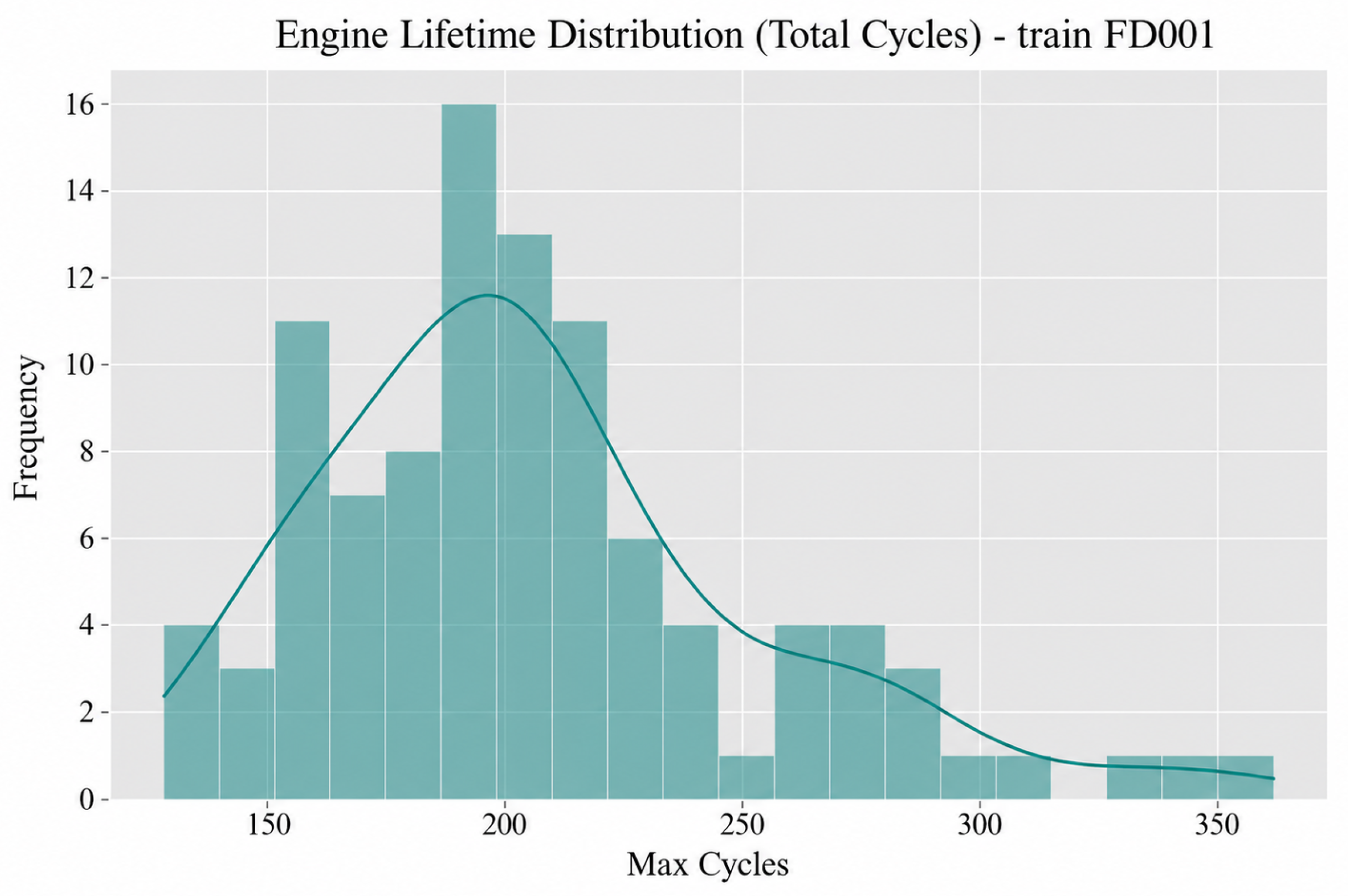
Figure 1 illustrates the distribution of total operating cycles for engine units in the FD001 training subset. It can be observed that engine lifetime is not uniformly distributed, but instead exhibits noticeable variability across different units, with most samples concentrated in the middle lifetime range and a relatively long tail extending toward higher cycle values. This indicates that the run-to-failure trajectories have unequal lengths, which makes direct fixed-size sequence learning infeasible without further sample standardization.
From a modeling perspective, this observation provides direct support for the use of window-based sample construction in this study. Since different engine units do not share the same degradation duration, a sliding-window strategy is needed to transform variable-length trajectories into fixed-length input samples while preserving local temporal continuity. In addition, the non-uniform lifetime distribution also suggests that degradation stages are not equally represented across the full trajectory space, which is relevant to the later maintenance-oriented health state partitioning. However, because the sliding-window segmentation described in Section 3.3.3 is applied strictly within each individual engine unit, engines with different total lifetimes each contribute temporal segments in proportion to their degradation trajectory length, so that engines concentrated in the average lifetime range do not disproportionately dominate the classification sample pool. The resulting window-level class distribution remains consistent and non-extreme across all four subsets, confirming that the labeling strategy produces a feasible class composition even under the observed skewed lifetime distribution. Furthermore, the use of Macro-F1 as the primary class-sensitive evaluation metric ensures that any residual class-frequency differences do not mask per-class recognition performance in the reported results.
To evaluate the proposed framework under different degradation complexities, all four subsets of the dataset, namely FD001, FD002, FD003, and FD004, are considered in this study. These subsets differ in the number of operating conditions and fault modes, thereby forming benchmark scenarios with different levels of difficulty. FD001 and FD003 correspond to single-operating-condition cases, whereas FD002 and FD004 involve multiple operating conditions and therefore exhibit stronger distributional heterogeneity. In addition, FD001 and FD002 contain one fault mode, while FD003 and FD004 contain two fault modes, which makes the latter subsets more challenging in terms of degradation pattern discrimination.
From the perspective of data composition, the four subsets together cover both relatively simple and more complex degradation environments. This design makes it possible to examine whether a predictive maintenance framework can maintain stable performance under different combinations of operating variability and fault diversity. Therefore, the use of FD001–FD004 together provides a comprehensive basis for studying the robustness and adaptability of maintenance-oriented health assessment methods. A summary of key subset characteristics is provided in Appendix A.

3.1.2. Maintenance-Oriented Problem Formulation

Unlike conventional C-MAPSS studies that formulate the task as continuous remaining useful life prediction, this work reformulates aero-engine degradation assessment as a maintenance-oriented health state classification problem. Specifically, each engine trajectory is mapped into three health states, namely Normal, Warning, and Fault, so that the output of the model becomes a maintenance alert label rather than a single numerical life estimate. Under this formulation, the prediction target is more directly connected to maintenance decision-making, since the three classes can naturally correspond to normal operation, early warning, and high-risk fault-prone conditions.
This reformulation is motivated by the practical observation that maintenance decisions are usually stage-oriented rather than purely value-oriented. Although continuous remaining useful life estimates can provide detailed degradation information, they are not always the most intuitive representation for operational use. In many real maintenance scenarios, decision makers are more concerned with whether an engine is operating normally, has entered a warning region, or requires immediate intervention. Therefore, transforming the degradation process into discrete health states improves the operational transparency and practical usefulness of the prediction output.
From a data representation perspective, the task remains based on sequential degradation observations rather than static samples. Each health state label is associated with a temporal segment of an engine trajectory, meaning that the classification decision is still driven by the historical evolution of operating settings and sensor signals. In this way, the task preserves the essential characteristics of degradation modeling while shifting the prediction target toward maintenance-oriented alert generation.

3.1.3. Overall Predictive Maintenance Framework

Based on the above data characteristics and task definition, an overall predictive maintenance framework is developed to convert raw C-MAPSS sequences into maintenance-decision-aligned alert outputs. The framework starts from the original multivariate time-series data and applies condition-aware preprocessing to reduce the interference caused by operating-condition variation. After that, degradation-sensitive features are generated and transformed into fixed-length temporal samples using a per-unit sliding window strategy. These samples are then fed into different predictive models to identify the corresponding health state of the engine. The final output is a three-class maintenance alert indicating whether the current operating condition should be regarded as Normal, Warning, or Fault.
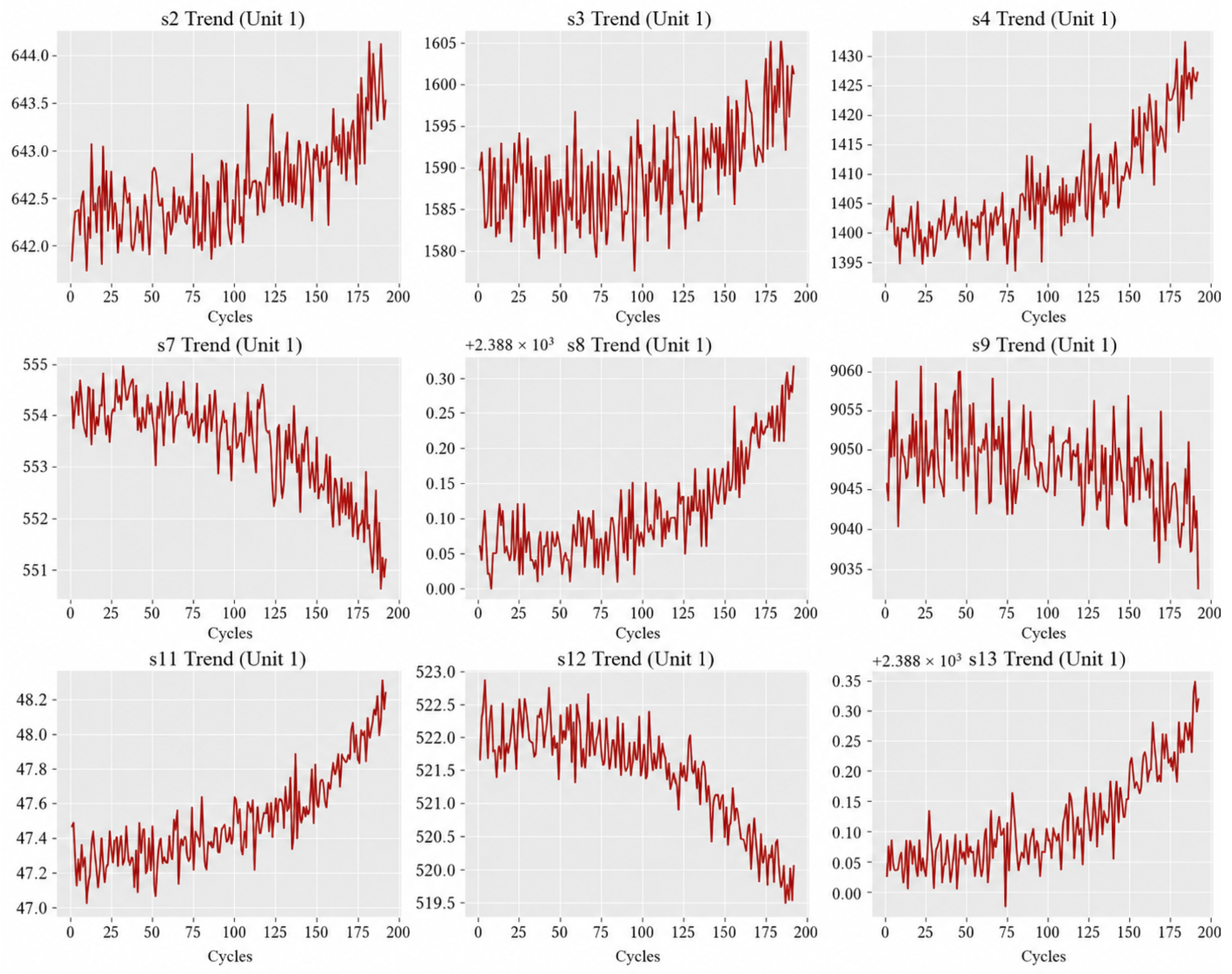
Figure 2 presents the temporal evolution of several representative sensors from a single engine unit. Clear trend differences can be observed across channels: some sensors exhibit progressive upward evolution, whereas others show gradual downward behavior as the number of cycles increases. Although short-term fluctuations are present, many channels still maintain directionally consistent long-term trends, indicating that the degradation process is reflected through multi-sensor temporal evolution rather than isolated instantaneous measurements.
This observation justifies the design of the proposed predictive maintenance framework from two aspects. First, it confirms that the health state of an engine should be modeled as a sequence-dependent process instead of a static classification problem. Second, it supports the introduction of differential features and temporal models in later sections, because the useful degradation information is not only contained in the sensor level itself, but also in the evolution direction and local rate of change over time.
Methodologically, the proposed framework consists of three main stages. The first stage is data preparation, which includes dataset organization, operating-condition adaptation, and temporal sample construction. The second stage is model development, where representative tree-based machine learning models and deep temporal models are established under a unified experimental setting. The third stage is maintenance-oriented output generation, in which the learned degradation patterns are translated into health state predictions for maintenance support. This pipeline forms a complete link from raw monitoring data to actionable maintenance information.
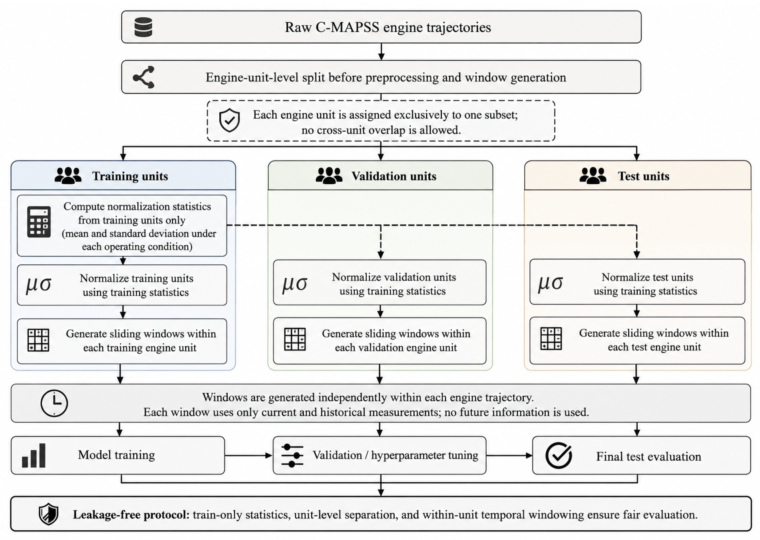
Figure 3 presents the complete data splitting and preprocessing workflow adopted in this study, illustrating how the leakage-free design is enforced at each stage of the pipeline.
As shown in Figure 3, the pipeline enforces a strict separation between training and test data at the engine-unit level, using the pre-partitioned C-MAPSS training and test files directly so that no engine unit appears in both partitions. Condition-regime statistics for normalization are estimated exclusively from the training trajectories and applied without modification to the test data, preventing any test-set influence on training-side preprocessing. Sliding-window segmentation is conducted strictly within each individual engine unit, ensuring that no window spans multiple units and that temporal continuity is not assumed across unit boundaries. These design choices collectively establish a leakage-free evaluation environment that supports reproducible cross-model comparison.
Overall, the framework is designed to preserve the temporal and operational characteristics of the original data while improving the operational transparency of the final prediction output. By integrating data description, maintenance-oriented task reformulation, and unified model evaluation into a single pipeline, the framework provides a systematic basis for condition-aware aero-engine predictive maintenance.

3.2. Health-State Labeling Strategy

The maintenance-oriented task reformulation requires each cycle of an engine trajectory to be assigned a discrete health state label. Because the C-MAPSS dataset provides a ground-truth remaining useful life value for each cycle, label assignment is performed by applying RUL-based thresholds that correspond to recognizable operational stages. Three health states are defined. Cycles with RUL greater than 80 cycles are assigned the Normal state, cycles with RUL in the range from 31 to 80 cycles inclusive are assigned the Warning state, and cycles with RUL of 30 cycles or below are assigned the Fault state. The selection of these boundaries is motivated by two considerations. First, the transition from Normal to Warning at RUL = 80 provides a sufficient lead time for maintenance planning, as engines in the Warning region exhibit observable degradation but are not yet in an immediately critical condition. Second, the Fault boundary at RUL = 30 captures cycles in which the engine is approaching the end of its operational life and requires prioritized intervention. These threshold values are consistent with commonly adopted RUL partitioning conventions in the C-MAPSS literature and are applied as a unified definition across all four benchmark subsets without modification. Table 2 summarizes the three health state labels, their corresponding RUL ranges, and their maintenance interpretations.
The same threshold setting was applied consistently to all four C-MAPSS subsets FD001–FD004 in order to avoid dataset-specific label definitions that could undermine cross-subset comparability. To verify that this unified setting produces a feasible class distribution for model training and evaluation, the number of window-level samples belonging to each health state was examined across all four subsets. Each window inherits the health state label of its last cycle, following the windowing convention described in Section 3.3.3. Table 3 reports the resulting label distribution.
As shown in Table 3, although the total number of windows differs across subsets due to differences in operating conditions and trajectory lengths, the distribution pattern of the three health states remains comparable across all four benchmark scenarios. The Normal class consistently represents approximately 47–50% of total windows, while the Warning and Fault classes account for approximately 30–31% and 20–21%, respectively. This distribution indicates that the proposed labeling strategy does not create an extreme class imbalance, and both the Warning and Fault classes contain sufficient samples for model training and evaluation across all subsets.
To examine whether the proposed framework is sensitive to the specific threshold setting, a sensitivity analysis was conducted by varying both RUL boundaries by ±10 cycles relative to the baseline. Three configurations were evaluated: a conservative setting with boundaries at 90 and 40 cycles, the baseline setting with boundaries at 80 and 30 cycles, and an aggressive setting with boundaries at 70 and 20 cycles. For each configuration, the best-performing model was retrained and evaluated on FD002, which is selected as the representative subset because it presents the highest classification difficulty among the four benchmarks, involving multiple operating conditions. Table 4 summarizes the classification performance under the three threshold settings.
As shown in Table 4, the baseline setting achieves the best overall performance, while the conservative and aggressive settings produce only limited degradation. The Macro-F1 score remains above 0.96 across all three threshold configurations. The Warning-class F1 score is the most sensitive indicator, decreasing by approximately 0.003 under the conservative setting and by approximately 0.006 under the aggressive setting relative to the baseline. Despite these variations, no configuration produces a substantial change in overall classification behavior. These results indicate that the proposed framework is not overly dependent on a specific threshold choice and that the main conclusions regarding model family comparison and preprocessing effectiveness hold robustly across reasonable variations in the health-state boundary definition.

3.3. Data Preprocessing and Feature Engineering

3.3.1. Condition-Wise Normalization Under Multiple Operating Regimes

The raw C-MAPSS data contain both degradation-related information and operating-conditioninduced variation. Since the same health state may produce different sensor responses under different operating regimes, direct global normalization may distort the true degradation patterns and weaken the discriminative ability of the subsequent models. Therefore, a condition-wise normalization strategy is adopted in this study to reduce operating-condition bias before feature learning.
Assume that the multivariate observation of the i-th engine at cycle t is represented as
x i , t = o i , t ( 1 ) , o i , t ( 2 ) , , o i , t ( p ) , s i , t ( 1 ) , s i , t ( 2 ) , , s i , t ( q ) R p + q
where o i , t ( k ) denotes the k-th operating setting and s i , t ( j ) denotes the j-th sensor measurement. Let the operating-condition label associated with cycle t of engine i be denoted by c i , t { 1 , 2 , , C } , where C is the number of identified operating regimes. In this study, the operating space is partitioned into several regimes according to the operating-setting variables, so that samples with similar operating characteristics are grouped together. In the C-MAPSS dataset, each cycle is accompanied by three operating setting variables that directly identify the active operating condition; the regime label c i , t is therefore assigned by matching these recorded setting values to predefined regime intervals, without requiring any unsupervised clustering or on-line condition inference. It should be noted that in a real-world deployment scenario where explicit operating condition labels are not directly available from the monitoring system, the regime assignment step would need to be replaced by an inference procedure based on available sensor telemetry, which constitutes an additional practical requirement not present in the benchmark evaluation.
For each sensor channel j within regime c, the mean and standard deviation are computed as
μ j ( c ) = 1 N c ( i , t ) : c i , t = c s i , t ( j ) σ j ( c ) = 1 N c ( i , t ) : c i , t = c s i , t ( j ) μ j ( c ) 2
where N c denotes the number of samples belonging to regime c. Then, condition-wise normalization is performed as
s ˜ i , t ( j ) = s i , t ( j ) μ j c i , t σ j c i , t + ε
where ε is a small positive constant introduced to avoid numerical instability when the variance is close to zero. Through this transformation, the scale and offset differences caused by operating-condition variation are reduced, making the normalized sensor variables more comparable across different regimes. In the experimental implementation, the regime-specific statistics μ j ( c ) and σ j ( c ) are estimated exclusively from the training trajectories and then applied without recomputation to the test data, ensuring that no test-set information influences the preprocessing of the training features. As a result, the subsequent feature extraction process can focus more on degradation behavior rather than condition-dependent fluctuation.
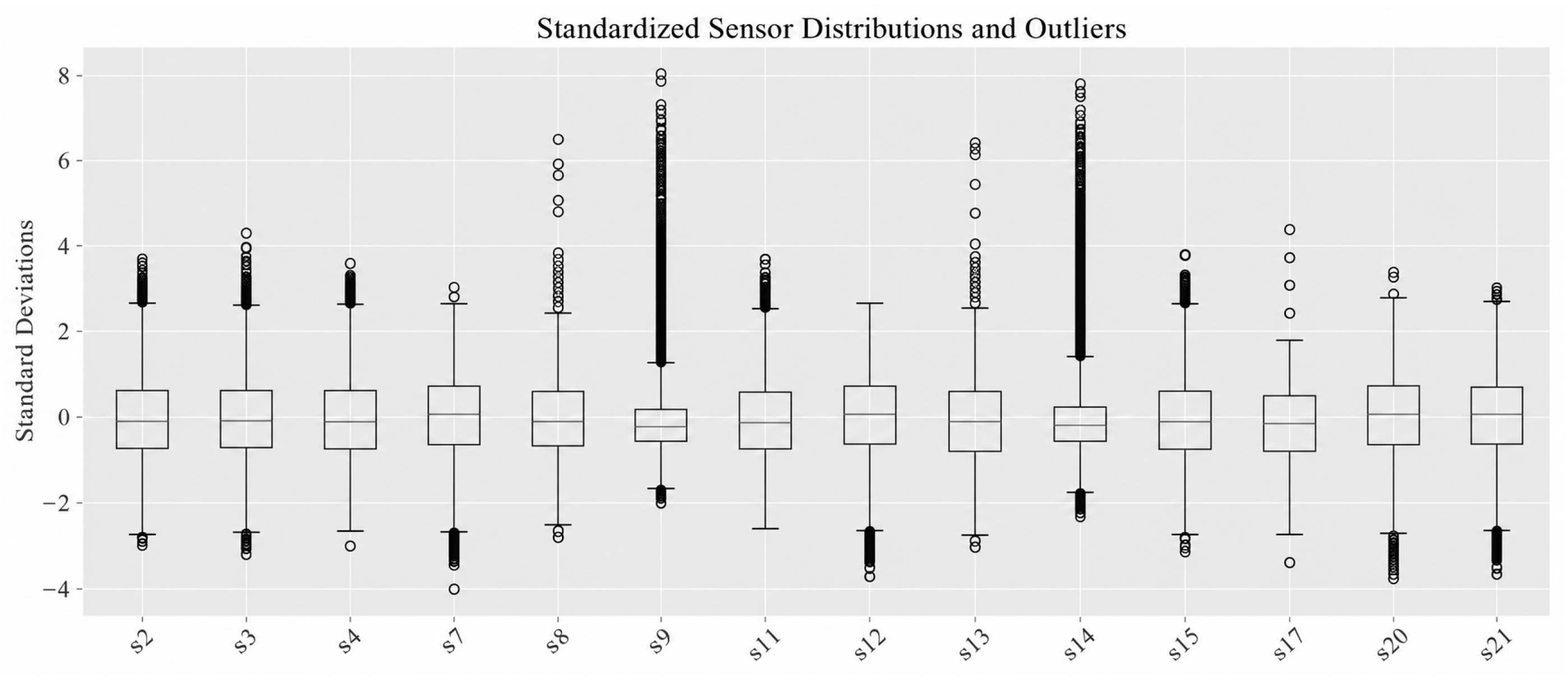
This phenomenon is important for subsequent model development. On the one hand, the improved alignment of sensor scales facilitates joint learning across channels and operating regimes. On the other hand, the remaining outliers suggest that the data still contain abrupt deviations, extreme degradation responses, or regime-sensitive fluctuations that should not be simply discarded. Therefore, the purpose of condition-wise normalization in this study is not to over-smooth the data, but to improve comparability while preserving potentially informative degradation signatures for downstream classification.
Figure 4 presents the standardized distributions of the selected sensor channels after normalization. It can be seen that the central ranges of different sensors become more comparable after scaling, which indicates that normalization effectively reduces the influence of inconsistent original measurement magnitudes. At the same time, noticeable outliers and heavy-tailed behavior remain in several channels, showing that normalization does not eliminate the underlying complexity of degradation-related signal variation.

3.3.2. Differential Feature Construction for Degradation Trend Characterization

Although normalized sensor values reflect the instantaneous operating state of the engine, they do not explicitly describe how the condition evolves over time. However, degradation is inherently a dynamic process, and the rate of change of sensor signals often provides additional information about the health transition of the system.
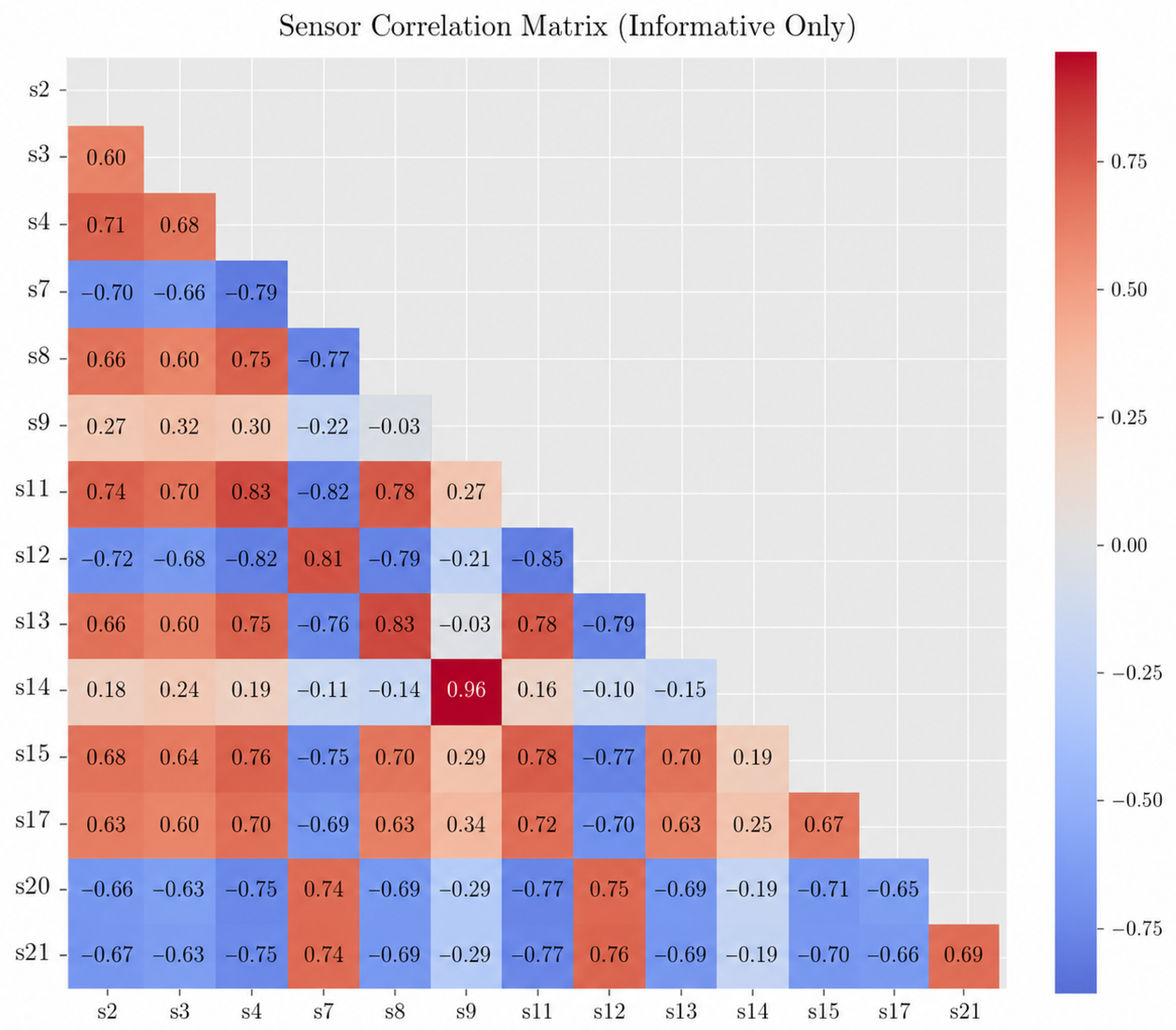
Figure 5 shows the correlation structure among the selected informative sensors. Strong positive and negative dependencies can be observed across multiple sensor pairs, indicating that degradation signatures are embedded in coupled multi-sensor variation rather than independent single-channel responses. In particular, several sensor groups form relatively stable correlation clusters, while others display strong inverse relationships, suggesting that the degradation process simultaneously drives different channels in different directions.
This correlation pattern has two implications for the present study. First, the selected sensors contain complementary yet partially redundant information, which supports joint multi-sensor modeling rather than isolated channel analysis. Second, because degradation is reflected not only in static sensor values but also in how correlated channels evolve together, the use of differential features is further justified. The first-order temporal difference helps expose local trend changes that may not be fully captured by raw normalized values alone, especially when multiple sensors respond synchronously or oppositely to the same degradation process.
To better capture this temporal evolution, first-order differential features are introduced as supplementary degradation descriptors.
For the j-th normalized sensor channel of engine i, the first-order temporal difference at cycle t is defined as
Δ s ˜ i , t ( j ) = s ˜ i , t ( j ) s ˜ i , t 1 ( j ) , t 2
This formulation approximates the local change rate of the sensor signal between two consecutive cycles. If s ˜ i , t ( j ) mainly characterizes the current state, then Δ s ˜ i , t ( j ) characterizes the local trend of degradation. The combination of these two types of information allows the model to distinguish not only whether the engine is currently in a certain state, but also whether it is moving toward a more severe state.
Accordingly, the feature vector at cycle t is augmented as
z i , t = s ˜ i , t , Δ s ˜ i , t R 2 q
where
s ˜ i , t = s ˜ i , t ( 1 ) , s ˜ i , t ( 2 ) , , s ˜ i , t ( q )
and
Δ s ˜ i , t = Δ s ˜ i , t ( 1 ) , Δ s ˜ i , t ( 2 ) , , Δ s ˜ i , t ( q )
This feature augmentation can be understood as enriching the representation from a static observation space to a joint state-trend space. In other words, the resulting features encode both the current degradation-sensitive measurement level and its short-term change direction, which is beneficial for maintenance-oriented health state discrimination.
Although finite differencing can amplify high-frequency noise in raw sensor signals, this effect is mitigated in the present framework by two design properties. First, the differential features are incorporated as part of the fixed-length temporal window rather than used as isolated single-cycle inputs; any cycle-to-cycle fluctuation is therefore contextualized by the surrounding observations within the window and does not independently determine the classification outcome. Second, the C-MAPSS dataset is generated from a controlled engineering simulation, and the sensor signals exhibit relatively smooth and gradual degradation trends with limited high-frequency stochastic variation, which substantially reduces the noise amplification risk compared with unfiltered real sensor streams. For deployment in environments with stronger sensor noise characteristics, a light pre-smoothing step applied prior to differencing may be warranted as an additional preprocessing measure.

3.3.3. Per-Unit Sliding Window Segmentation and Label Representation

The C-MAPSS data are sequential degradation trajectories, and the health state of an engine at a given cycle depends not only on the current observation but also on its recent temporal history. Therefore, instead of using cycle-wise independent samples, this study adopts a per-unit sliding window strategy to construct fixed-length temporal segments. This approach preserves local temporal continuity and enables the models to learn degradation patterns from consecutive observations.
For engine i, let its processed feature sequence be denoted by
Z i = z i , 1 , z i , 2 , , z i , T i
where T i is the total number of cycles of engine i. Given a window length L, the k-th sample generated from engine i is defined as
X i , k = z i , k , z i , k + 1 , , z i , k + L 1 R L × 2 q
with
k = 1 , 2 , , T i L + 1
Because the windowing procedure is conducted strictly within each engine unit, samples from different engines are never concatenated into the same temporal segment. This avoids cross-unit information leakage and ensures that each training sample corresponds to a physically consistent degradation fragment.
The label assigned to each window is determined by the health state associated with the end cycle of the window. Let y i , t     { 0 , 1 , 2 } denote the class label at cycle t, corresponding to Normal, Warning, and Fault, respectively. Then, the label of X i , k is defined as
Y i , k = y i , k + L 1
This strategy is based on the assumption that the most recent cycle in the window provides the target health state to be identified, while the preceding cycles provide temporal context for the prediction. Consequently, the sample-label pair can be written as
X i , k , Y i , k
which forms the basic input-output unit for subsequent classification models.
From a maintenance perspective, this window-based representation is particularly appropriate because maintenance alerts are rarely triggered by a single isolated measurement. Instead, they are typically determined from short-term degradation evolution over a recent operating horizon. By converting the original trajectories into fixed-length temporal segments with end-of-window labels, the proposed preprocessing pipeline establishes a consistent representation for both tree-based models and deep temporal models, thereby enabling a unified comparison of different predictive maintenance strategies.

3.4. Model Development

3.4.1. Tree-Based Machine Learning Models

Tree-based machine learning models are adopted in this study as representative structured-data baselines for maintenance-oriented health state classification. Their inclusion is motivated by two considerations. First, after condition-wise normalization, differential feature construction, and sliding-window segmentation, the original sequential monitoring data can be transformed into informative feature representations that are suitable for tabular learning. Second, tree-based models are well known for their strong nonlinear fitting ability, robustness to heterogeneous feature scales, and competitive performance on small-to-medium-sized industrial datasets. Therefore, they provide an important reference for evaluating whether more complex temporal neural models are necessary for the present task.
Given a window sample X i , k R L × 2 q , a fixed-dimensional vector representation is constructed before being fed into tree-based classifiers. Let the flattened representation of the window be denoted by
v i , k = vec X i , k
where v i , k R 2 qL . The corresponding classification target is the health state label Y i , k { 0 , 1 , 2 } , which represents the Normal, Warning, and Fault classes, respectively. Under this formulation, the tree-based model learns a mapping
f tree : R 2 qL { 0 , 1 , 2 }
so that the predicted class of a sample can be written as
Y ^ i , k = f tree v i , k
In this study, three representative tree-based classifiers are considered, namely Random Forest, XGBoost, and LightGBM. Random Forest serves as a robust ensemble baseline by aggregating the predictions of multiple decision trees constructed from bootstrapped samples and random feature subsets. Its prediction can be expressed as a majority-voting function
Y ^ i , k = mode h 1 v i , k , h 2 v i , k , , h M v i , k
where h m ( · ) denotes the m-th decision tree and M is the total number of trees. In contrast, XGBoost and LightGBM are gradient-boosting frameworks that construct additive tree ensembles in a stage-wise manner. Their predictive function can be written in the general form
F v i , k = m = 1 M f m v i , k
where f m ( · ) denotes the m-th boosted tree. For classification, the final class label is obtained by selecting the category with the highest predicted score
Y ^ i , k = arg max c { 0 , 1 , 2 } F c v i , k
These models are particularly suitable for verifying whether the engineered feature space already contains sufficient degradation-sensitive information for reliable maintenance alert generation.

3.4.2. Deep Temporal Models

Although tree-based models can capture nonlinear relationships in flattened window features, they do not explicitly model the temporal ordering within each degradation segment. However, aeroengine degradation is inherently sequential, and the health state at the current cycle is closely related to the recent temporal evolution of sensor responses. For this reason, deep temporal models are introduced to learn health representations directly from ordered sequence inputs. In this study, two representative neural architectures are considered, namely a context-aware multi-scale temporal attention convolutional neural network and a bidirectional long short-term memory network.
For deep temporal modeling, each sample is directly represented by its window tensor
X i , k = x i , k ( 1 ) , x i , k ( 2 ) , , x i , k ( L )
where x i , k ( t ) R 2 q denotes the feature vector at the t-th position within the window. The deep model learns a nonlinear mapping
f deep : R L × 2 q R 3
which produces a three-dimensional output score vector
o i , k = f deep X i , k
The posterior probability of class c is then obtained through the softmax transformation
P Y i , k = c X i , k = exp o i , k ( c ) r = 0 2 exp o i , k ( r )
and the predicted health state is determined as
Y ^ i , k = arg max c { 0 , 1 , 2 } P Y i , k = c X i , k
The context-aware MSTA-CNN is designed to extract local temporal patterns at multiple receptive scales. Its convolutional branches operate on the input sequence using kernels of different lengths so that short-term fluctuations and medium-range degradation cues can be captured simultaneously. Let ϕ r X i , k denote the feature map extracted by the r-th convolutional branch. The multi-scale representation can be expressed as
H i , k cnn = Concat ϕ 1 X i , k , ϕ 2 X i , k , , ϕ R X i , k
where R is the number of convolutional branches. To improve sensitivity to informative temporal regions, an attention weighting mechanism is further introduced. Let the attention weight at temporal position t be α t , satisfying
t = 1 L α t = 1
Then the aggregated temporal representation is given by
g i , k cnn = t = 1 L α t h i , k , t cnn
where h i , k , t cmn denotes the hidden feature vector at temporal position t. This mechanism allows the model to emphasize degradation stages that are more relevant to maintenance alert prediction.
The Bi-LSTM model is adopted to capture bidirectional temporal dependencies within each degradation segment. Let h t and h t denote the forward and backward hidden states at step t t respectively. Their concatenation forms the bidirectional temporal representation.
h t = Concat h t , h t
The final sequence representation can be obtained either from the last hidden state or from an aggregated hidden representation over the full window. In this study, the temporal representation is further transformed by a fully connected layer to generate the output score vector o i , k . Compared with convolutional structures, Bi-LSTM is better suited to preserving progressive and cumulative degradation information over longer horizons, which is particularly relevant for maintenance oriented health state discrimination.

3.4.3. Training Strategy and Implementation Details

To ensure a fair comparison among different model families, all classifiers are trained under a unified data preparation and evaluation framework. Specifically, the same condition-wise normalization, differential feature construction, and per-unit sliding-window segmentation procedures are applied before model training. All models are trained to predict the same three-class health state target, and their performance is evaluated on the same C-MAPSS subsets. This unified setting allows the observed performance differences to be attributed mainly to modeling capability rather than inconsistent preprocessing conditions.
For the neural models, the optimization objective is the multi-class cross-entropy loss. Let the onehot encoded label of sample (i,k) be denoted by y i , k { 0 , 1 } 3 , and let the predicted class probability vector be p i , k . The loss over a training set containing N samples is defined as
L = 1 N n = 1 N c = 0 2 y n ( c ) log p n ( c )
where y n ( c ) and p n ( c ) denote the ground-truth indicator and predicted probability of class c for the n th sample. The model parameters are optimized by minimizing L over the training data. This loss function is suitable for the present task because it directly promotes correct discrimination among the three maintenance alert states.
Overall, the model development strategy follows a clear comparative logic. Tree-based models are used to assess the effectiveness of the engineered feature space under structured classification, while deep temporal models are used to investigate whether explicit sequential modeling provides additional benefit for the same task. Through this design, the study establishes a complete and consistent modeling framework for comparing different predictive maintenance strategies on the CMAPSS benchmark.

4. Results

4.1. Experimental Settings

All experiments were conducted under the unified leakage-free workflow described in Section 3 and illustrated in Figure 3. The experimental procedure consisted of three consecutive stages. First, the original monitoring data were transformed into condition-adapted and degradation-sensitive samples through the preprocessing pipeline. Second, five representative models, namely XGBoost, LightGBM, Random Forest, MSTA-CNN, and Bi-LSTM, were trained on the preprocessed training windows under the same three-class health state classification setting. Third, the trained models were evaluated on the corresponding test windows using a consistent set of classification metrics. This unified design ensures that the observed performance differences mainly reflect model capability rather than inconsistencies in data processing or target definition.
To assess the statistical stability of the neural network models, Bi-LSTM and MSTA-CNN were each trained under five different random seeds on the FD002 validation partition, which is the same held-out split used in the ablation study. Tree-based models, namely Random Forest, XGBoost, and LightGBM, were evaluated under fixed hyperparameters and a fixed random seed; because their training procedures are deterministic given the same data and configuration, repeated-run variability analysis is directed primarily at the neural network models, whose results are more sensitive to random initialization and stochastic mini-batch optimization. Table 5 reports the mean, standard deviation, and 95% confidence interval of the main classification metrics over the five repeated runs.
As shown in Table 5, both neural network models exhibit small run-to-run variation, with standard deviations in Macro-F1 not exceeding 0.004 and 95% confidence intervals spanning approximately 0.010. These results indicate that the reported neural-network performance is relatively stable under different random initializations. However, because the performance margins among several candidate models in this benchmark remain within a few percentage points, the present study avoids claiming statistically definitive superiority of any single model family, and the comparisons reported in the following sections should be interpreted as indicative of performance trends rather than conclusive rankings.

4.2. Overall Performance Comparison Across Models and Datasets

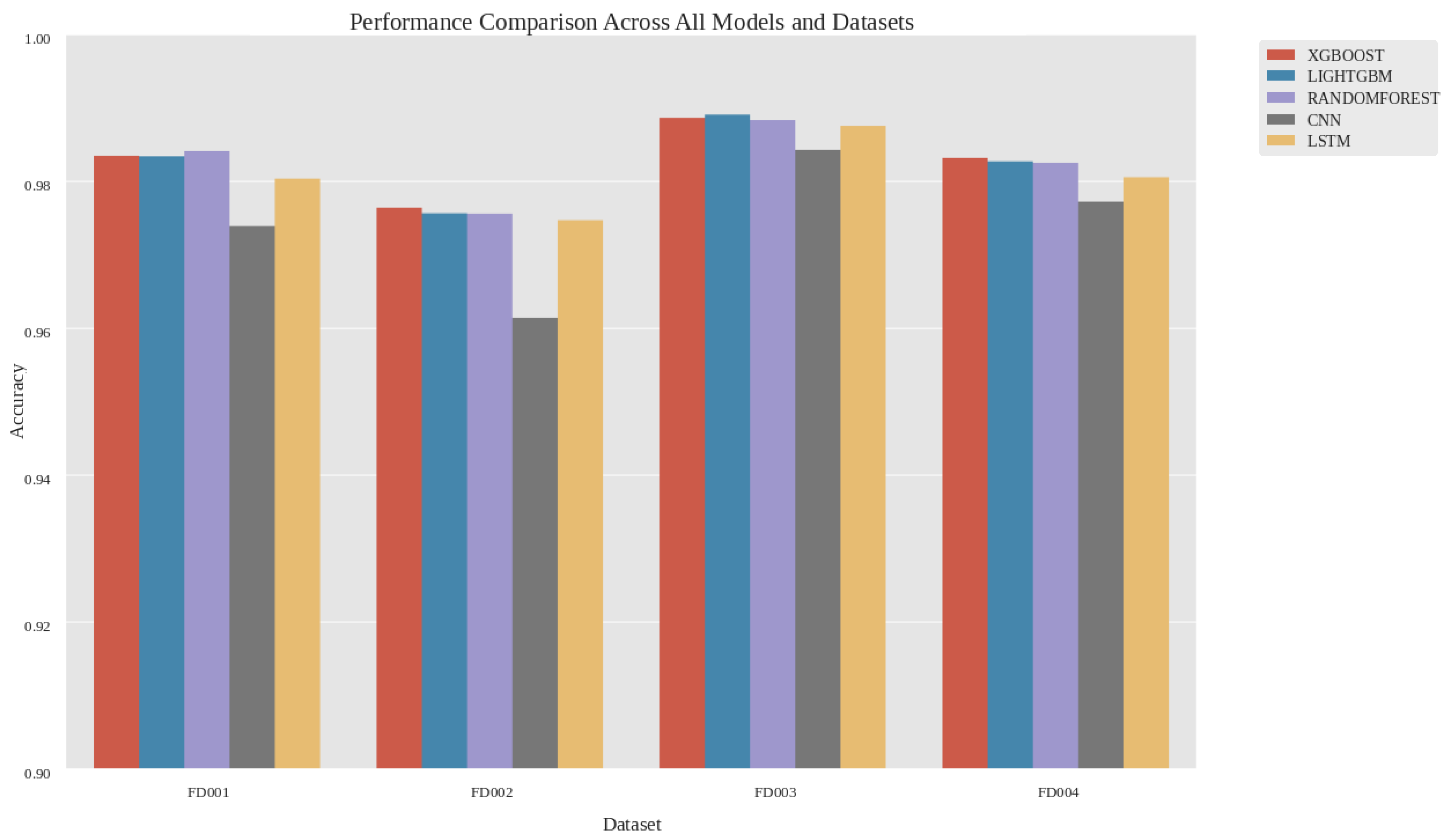
The overall accuracy results show that all five models achieve high classification performance on the four C-MAPSS subsets, indicating that the proposed maintenance-oriented task formulation is feasible for C-MAPSS-based health state assessment. However, clear differences can be observed among model families. Tree-based models generally occupy the leading positions, while the Multi-Scale Temporal Attention CNN (MSTA-CNN) achieves the lowest accuracy among the five evaluated models on all subsets. For clarity, the terms “CNN-based model” and “CNN-based architecture” used in the following figures and family-level comparisons all refer to this same MSTA-CNN model.
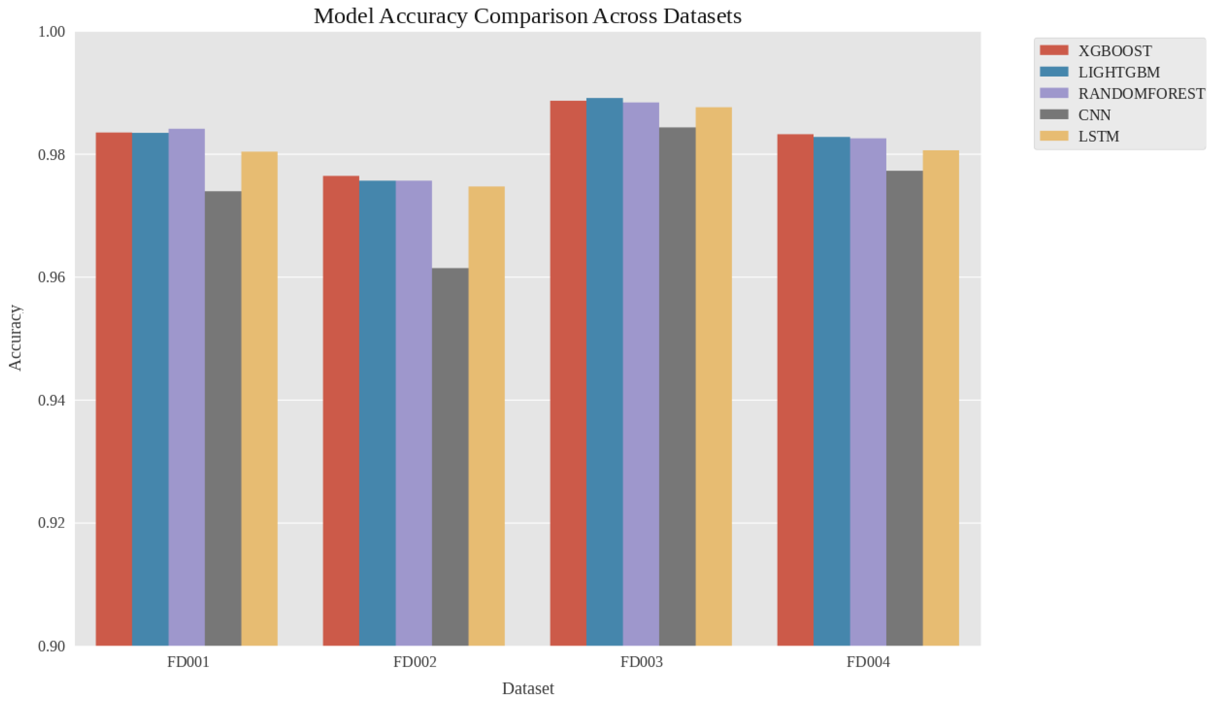
As shown in Table 6, the best results on FD001, FD002, FD003, and FD004 are achieved by Random Forest, XGBoost, LightGBM, and XGBoost, respectively. The corresponding accuracies are 0.9841, 0.9764, 0.9891, and 0.9832. These results indicate that tree-based models generally achieve the highest accuracy in this evaluation, with the best tree-based model outperforming Bi-LSTM by 0.0015 to 0.0037 across the four subsets.
As shown in Figure 6, the accuracy comparison reveals a consistent performance ranking across the four benchmark subsets. Tree-based models, especially XGBoost, LightGBM, and Random Forest, achieve the highest accuracy levels across all subsets, whereas MSTA-CNN achieves the lowest accuracy in all cases. This is consistent with the proposed preprocessing pipeline producing a discriminative structured feature space that particularly benefits ensemble tree models.
From the dataset perspective, FD003 yields the highest accuracy and FD002 the lowest across all five models. This pattern is consistent with the hypothesis that task difficulty is influenced by the complexity of the underlying operating conditions and degradation environment. The relatively lower results on FD002 suggest that multi-condition settings introduce additional classification ambiguity that is not fully resolved by condition-aware preprocessing alone.
The F1-score results exhibit a ranking pattern broadly consistent with the accuracy results, which supports the reliability of the overall conclusion. Tree-based models again occupy the top positions in the comparison, while Bi-LSTM consistently outperforms MSTA-CNN. This cross-metric consistency suggests that the performance differences among the leading models are not caused merely by class-distribution bias, but are also reflected in class-sensitive discrimination behavior.
Table 7 further shows that MSTA-CNN achieves stable multi-metric performance across FD001–FD004, although it remains lower than the best-performing tree-based models and Bi-LSTM on all subsets. Its highest accuracy is observed on FD003, while FD002 remains the most challenging subset.
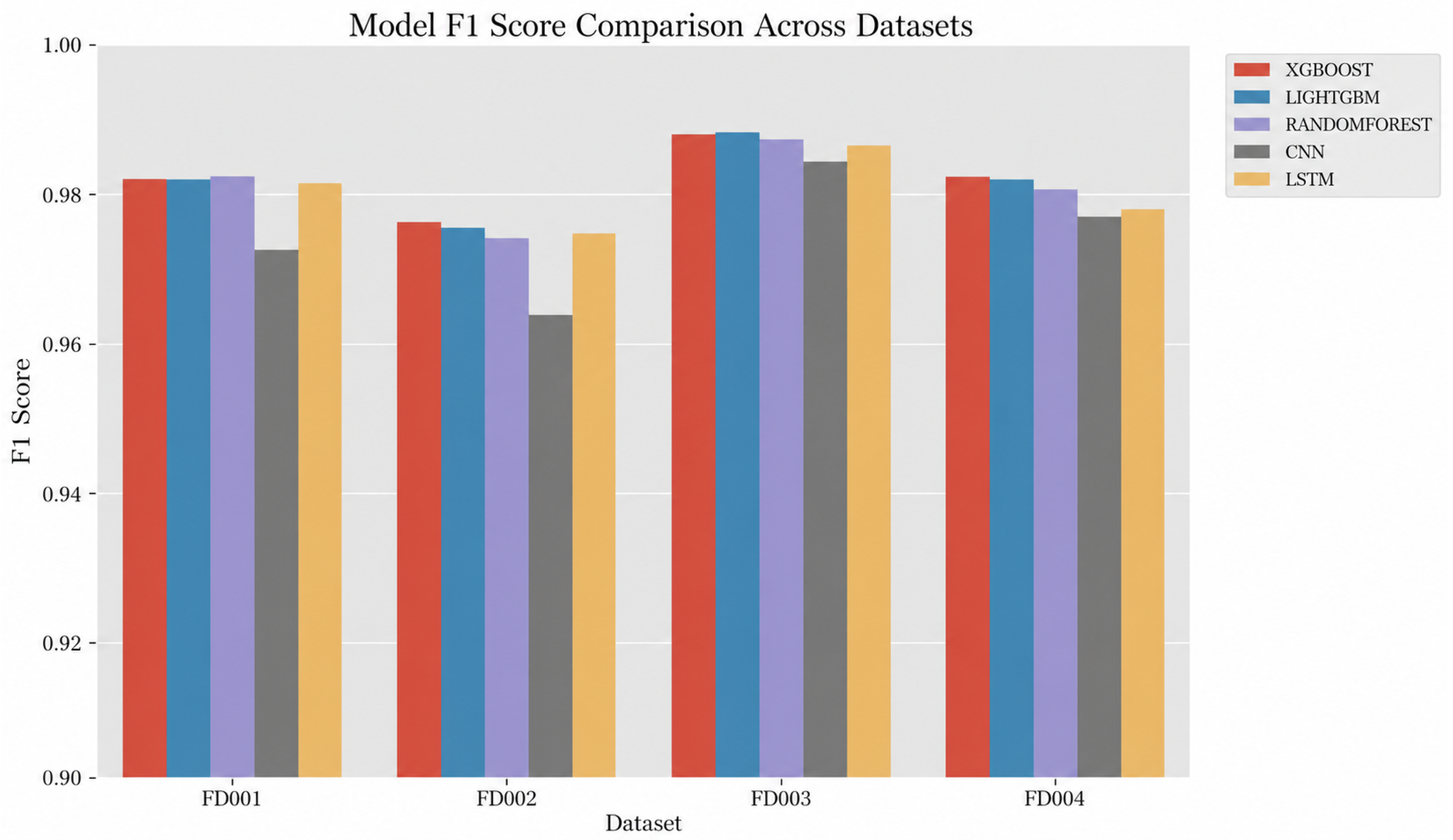
As shown in Figure 7, the F1-score comparison further verifies the performance pattern observed in the accuracy results. The ranking of the five models remains largely unchanged, with tree-based models continuing to occupy the top positions and Bi-LSTM consistently outperforming MSTA-CNN. This cross-metric consistency suggests that the performance differences among the leading models are not primarily attributable to majority-class bias, but are also reflected in balanced discrimination across the three maintenance states.
Compared with accuracy alone, the F1-score provides a more informative view of class-sensitive performance because it reflects the balance between precision and recall. The close agreement between the two metrics suggests that the proposed framework performs reliably not only in terms of overall correctness but also in terms of maintaining relatively balanced recognition ability across Normal, Warning, and Fault classes. This is particularly important for predictive maintenance, where weak recognition of transitional or high-risk classes would reduce practical usefulness even if global accuracy remained high.
Another observation is that the gap between Bi-LSTM and MSTA-CNN is apparent under F1-score evaluation. This is consistent with the view that long-term temporal dependency modeling provides additional benefit over local convolutional pattern extraction for the present task. The F1-score results therefore offer complementary support for the relevance of temporal sequence modeling in maintenance-oriented health assessment.
As shown in Figure 8, the overall benchmark comparison provides a compact summary of the performance relationships among models and datasets. Three key observations can be drawn. First, all five models achieve high classification performance across all benchmark subsets, indicating that the maintenance-oriented reformulation is feasible under the present benchmark conditions. Second, the top-performing models in each subset belong to the tree-based family, which is consistent with condition-aware preprocessing and degradation-sensitive feature construction exposing a discriminative structured feature space that benefits ensemble methods. Third, among the deep learning models, Bi-LSTM shows a consistent advantage over MSTA-CNN, suggesting that long-range temporal dependency provides additional benefit over local convolutional feature extraction for this task.
This benchmark-level view moves the analysis beyond individual subset results and reveals a stable family-level ranking. Rather than relying on a single winning model, the results show that the proposed pipeline supports multiple competitive classifiers, which suggests that the observed performance is attributable not only to model selection but also to the joint design of task formulation, preprocessing, and representation strategy.
From a predictive maintenance perspective, this comparison suggests that the framework supports maintenance-oriented health assessment under different degradation scenarios in this benchmark setting. It also indicates that future improvements are more likely to come from better transitional-state modeling and calibration rather than from simply replacing one model family with another.
These findings suggest that the preprocessing and feature construction steps transform the original degradation sequences into a representation that exposes class-relevant variation in a way that benefits classification. The final performance is therefore not solely attributable to model complexity, but also to the quality of the input representation. This is a practically relevant observation because it implies that performance gains in maintenance-oriented health assessment can be pursued through better data preparation alongside advances in model architecture.

4.3. Ablation Study of Framework Components

To quantify the individual contribution of each preprocessing and modeling component, an ablation study was conducted on the FD002 subset, which represents the most challenging scenario in the benchmark due to its multiple operating conditions. To avoid introducing additional test-set dependency, the ablation experiments were performed on a held-out validation partition drawn from the FD002 training trajectories, using 80% of engine units for model fitting and the remaining 20% for validation. Five ablation variants were evaluated by systematically removing one component at a time from the full framework: Variant A removes condition-wise normalization and replaces it with global standardization; Variant B removes first-order differential features so that the model receives only static normalized sensor values; Variant C removes per-unit sliding window segmentation and replaces it with single-cycle independent samples; Variant D replaces the Bi-LSTM temporal model with a non-sequential classifier that treats the flattened window as an unordered feature vector; and Variant E removes all four components simultaneously to provide a minimal baseline. The Bi-LSTM network serves as the reference architecture for the temporal modeling comparison. Table 8 reports the classification performance of the full framework and the five ablation variants.
As shown in Table 8, all four components provide measurable and consistent contributions to the overall classification performance. Per-unit sliding window segmentation and condition-wise normalization produce the largest individual degradation when removed, with accuracy drops of 0.016 and 0.013, respectively, and proportionally larger decreases in Warning-class F1. This indicates that preserving temporal continuity within engine-specific degradation fragments and eliminating operating-condition-induced distributional bias are both critical for reliable health state discrimination in the multi-condition environment of FD002. The contribution of first-order differential features is more moderate, with an accuracy drop of 0.008 when removed, yet the reduction in Warning F1 remains notable, confirming that explicit local degradation trend information provides meaningful supplementary signal beyond static normalized sensor values alone. The temporal modeling component also shows a consistent positive effect, with a 0.007 accuracy drop when Bi-LSTM is replaced by a non-sequential classifier, reinforcing the value of sequential dependency modeling given the cumulative and order-sensitive nature of aero-engine degradation. Finally, Variant E, which removes all components simultaneously, exhibits the largest overall degradation across all metrics, indicating that the individual contributions are not redundant but instead address complementary aspects of the health representation problem. These ablation results collectively confirm that the effectiveness of the proposed framework arises from the joint design of its preprocessing and modeling components rather than from any single element in isolation.

4.4. Class-Level Error Analysis Based on Confusion Matrices

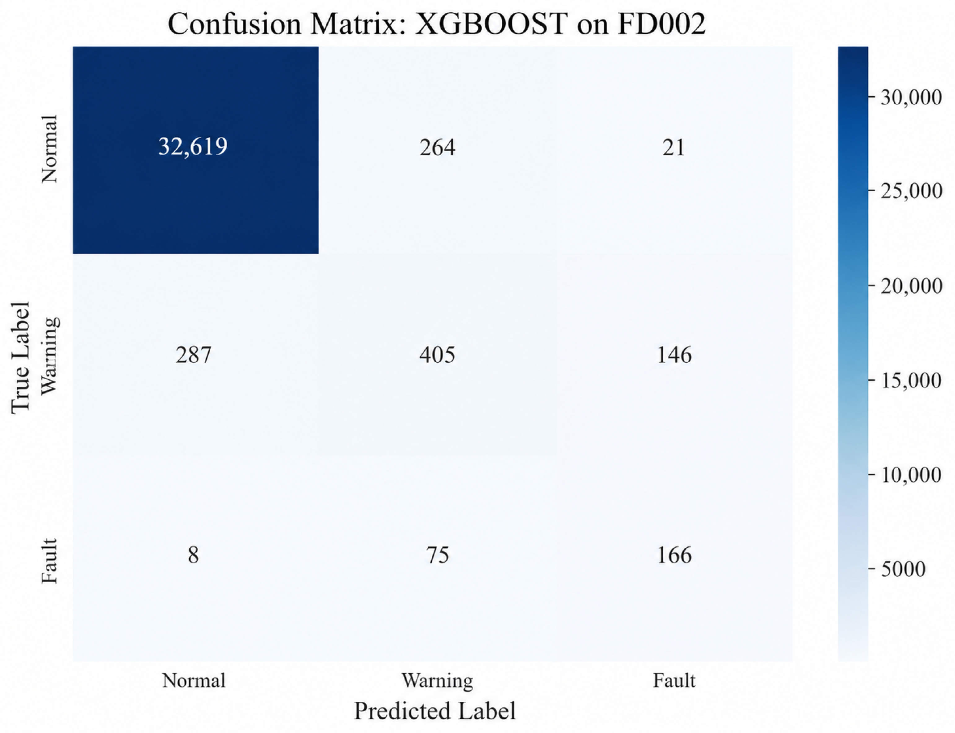
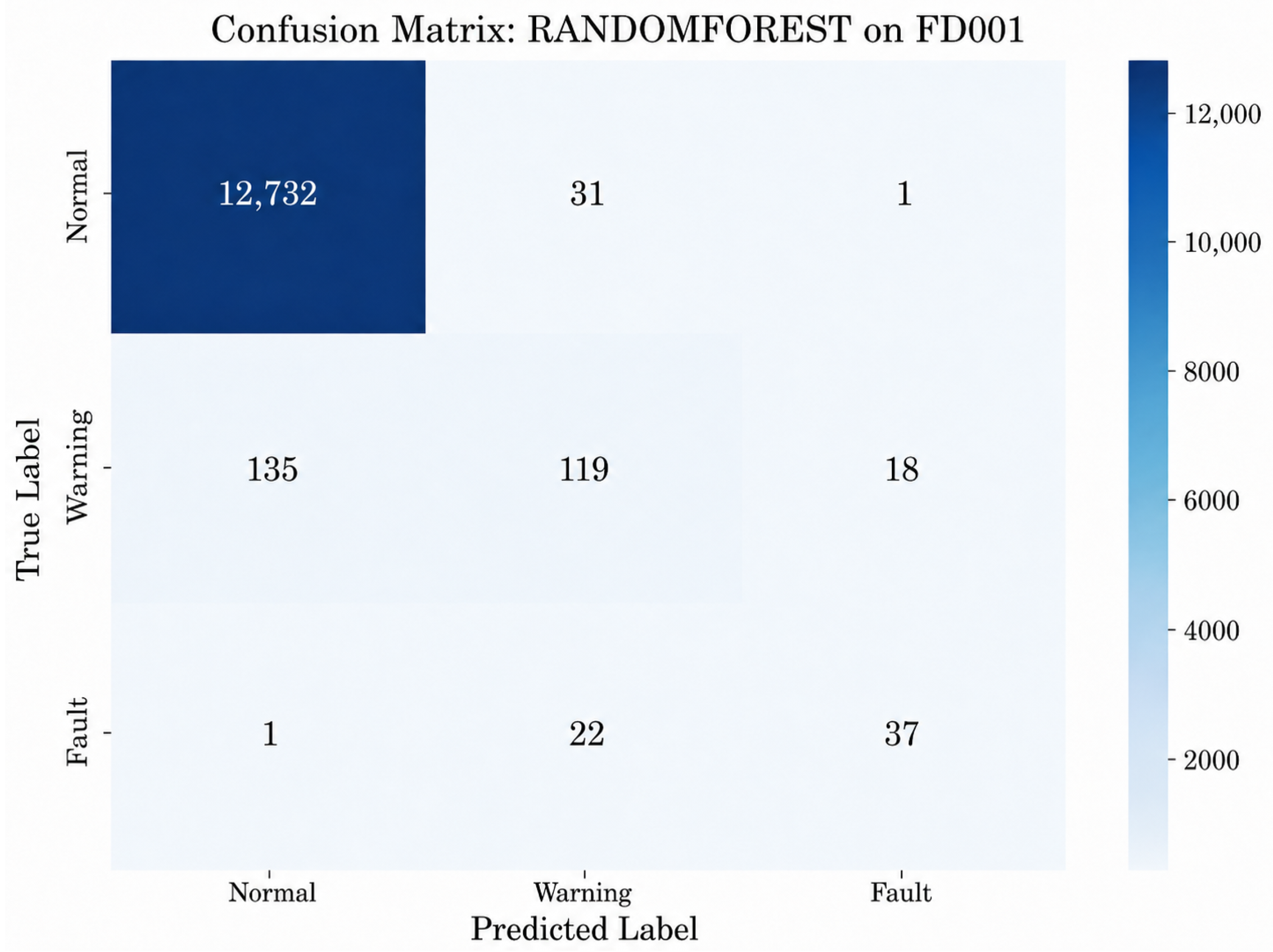
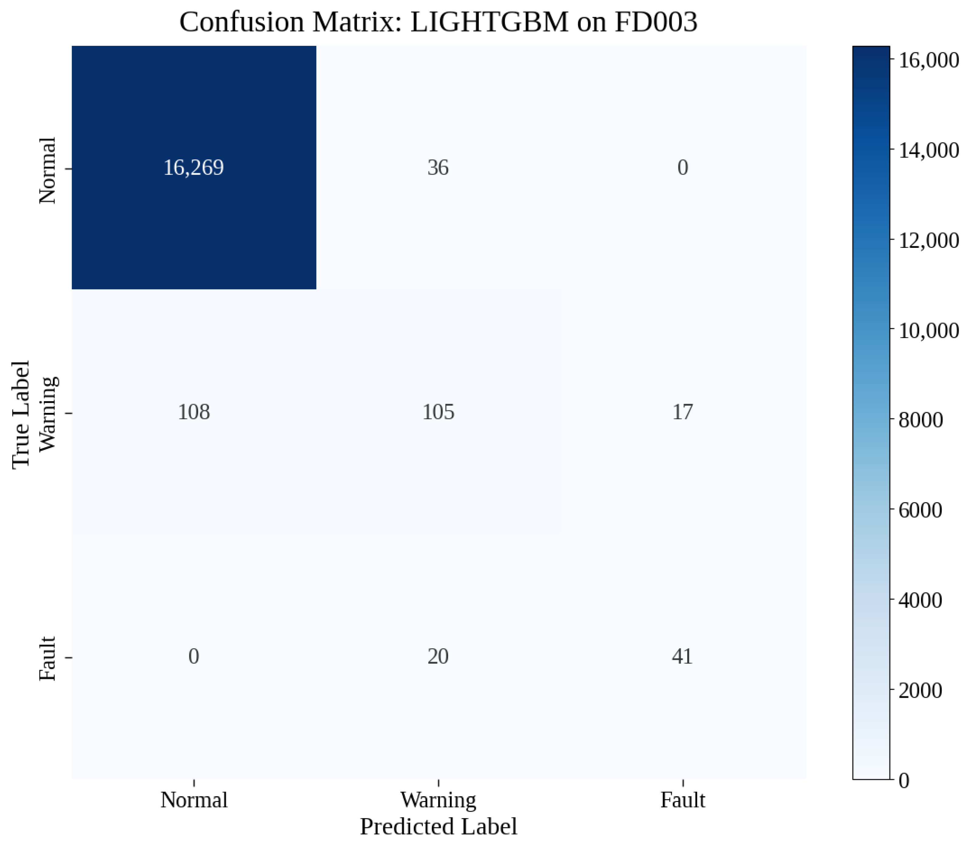
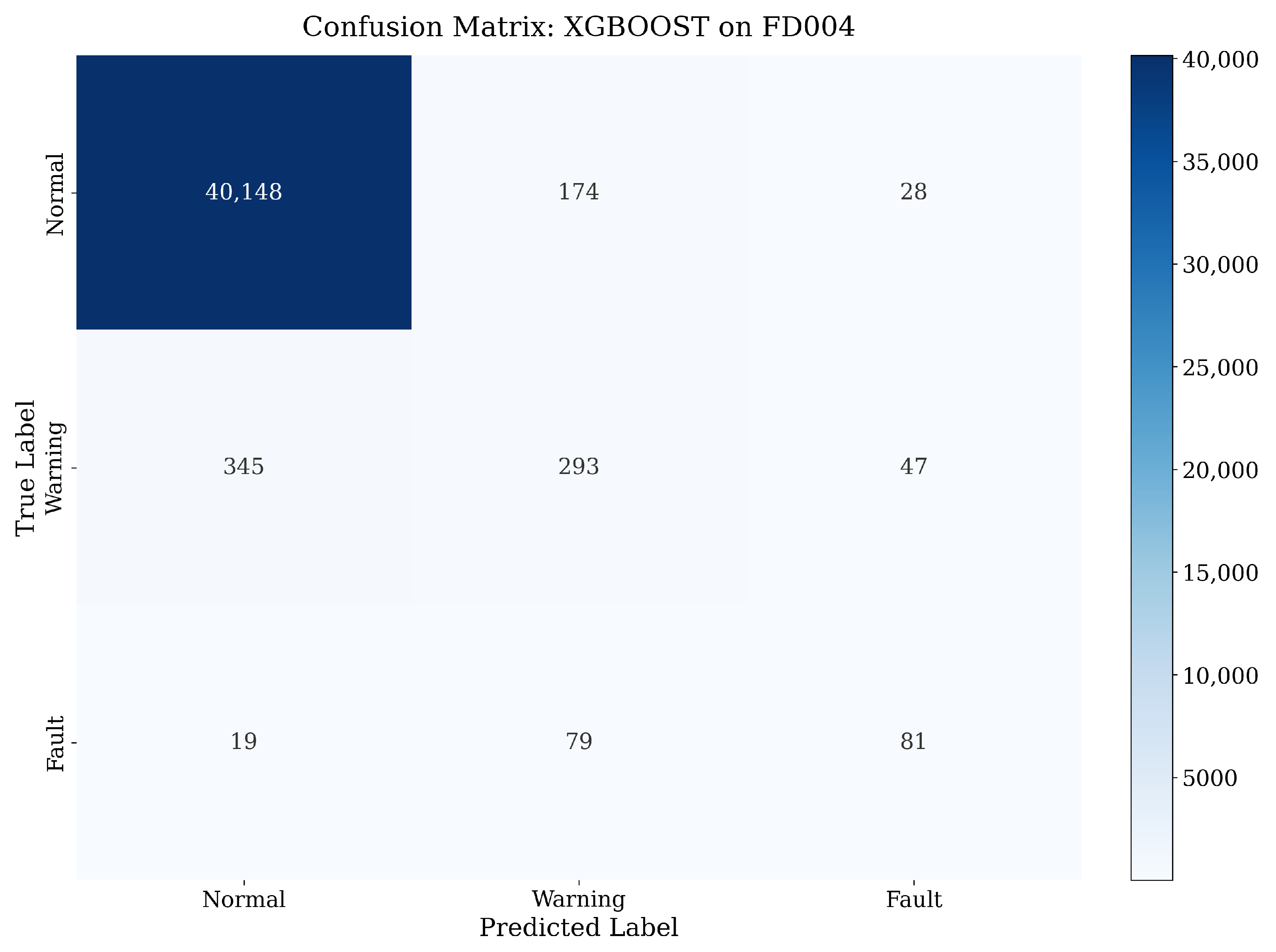
The confusion-matrix analysis of the best-performing model on each subset reveals a common structural pattern across all four datasets. As shown in Figure 9, Figure 10, Figure 11 and Figure 12, the diagonal entries for the Normal class are consistently the largest in each row, reflecting high per-class accuracy. Direct confusion between Normal and Fault is limited in all four subsets, indicating that the framework is effective at distinguishing the two outer health states. The Warning class, by contrast, shows the most off-diagonal entries in each confusion matrix, confirming that the transitional degradation stage is the primary source of classification difficulty.
As shown in Figure 9 and Figure 10, the confusion matrices for FD001 and FD002 show diagonal-dominant patterns for all three classes. In both subsets, the Normal class achieves high diagonal frequency, and Normal-to-Fault and Fault-to-Normal misclassifications are limited. The two outer health states are therefore more separable than the transitional Warning class, which is the expected pattern in maintenance-oriented classification.
At the same time, the two subsets reveal different levels of classification difficulty. Compared with FD001, FD002 shows a more pronounced off-diagonal concentration around the Warning class, reflecting the stronger distributional overlap introduced by multiple operating conditions. These two confusion matrices together illustrate both the general pattern of the framework and the influence of dataset complexity on class-level discrimination.
As shown in Figure 11 and Figure 12, the confusion patterns on FD003 and FD004 further confirm that the Warning state is the most difficult class to distinguish, even when the overall classification performance remains high. In FD003, the diagonal dominance is particularly strong, indicating relatively clear class separation, yet the remaining off-diagonal entries still concentrate mainly around the Warning class. In FD004, the overlap between Warning and its neighboring states becomes more noticeable, reflecting the increased challenge of maintenance-oriented classification under more complex degradation conditions.
These two confusion matrices further confirm that the principal difficulty of the task lies in identifying the transitional Warning region rather than separating Normal from Fault. The framework performs more reliably for the two outer health states than for the Warning class, and the main room for improvement lies in better characterization of borderline warning conditions.
In contrast, the most substantial misclassification occurs in the Warning class. Across all four subsets, Warning samples are more frequently confused with both Normal and Fault than either of the two outer states are confused with each other. This pattern is particularly evident in FD002 and FD004, where a noticeable proportion of Warning samples is predicted as Normal, and a smaller but still meaningful portion is predicted as Fault. Such behavior is consistent with the role of Warning as an intermediate degradation stage located near the decision boundary between health and failure-prone conditions.

4.5. Class-Wise Discriminative Ability Based on ROC Curves

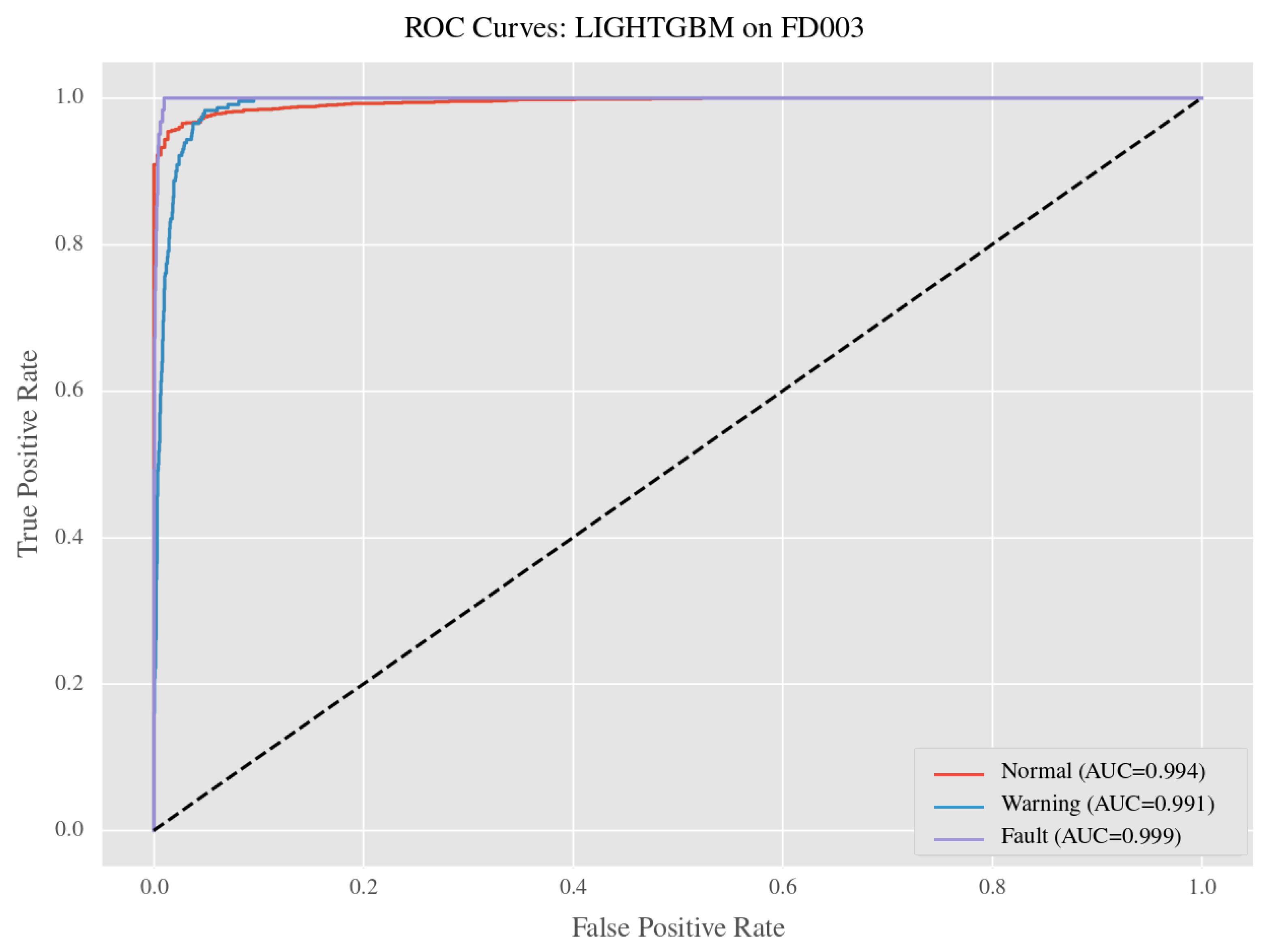
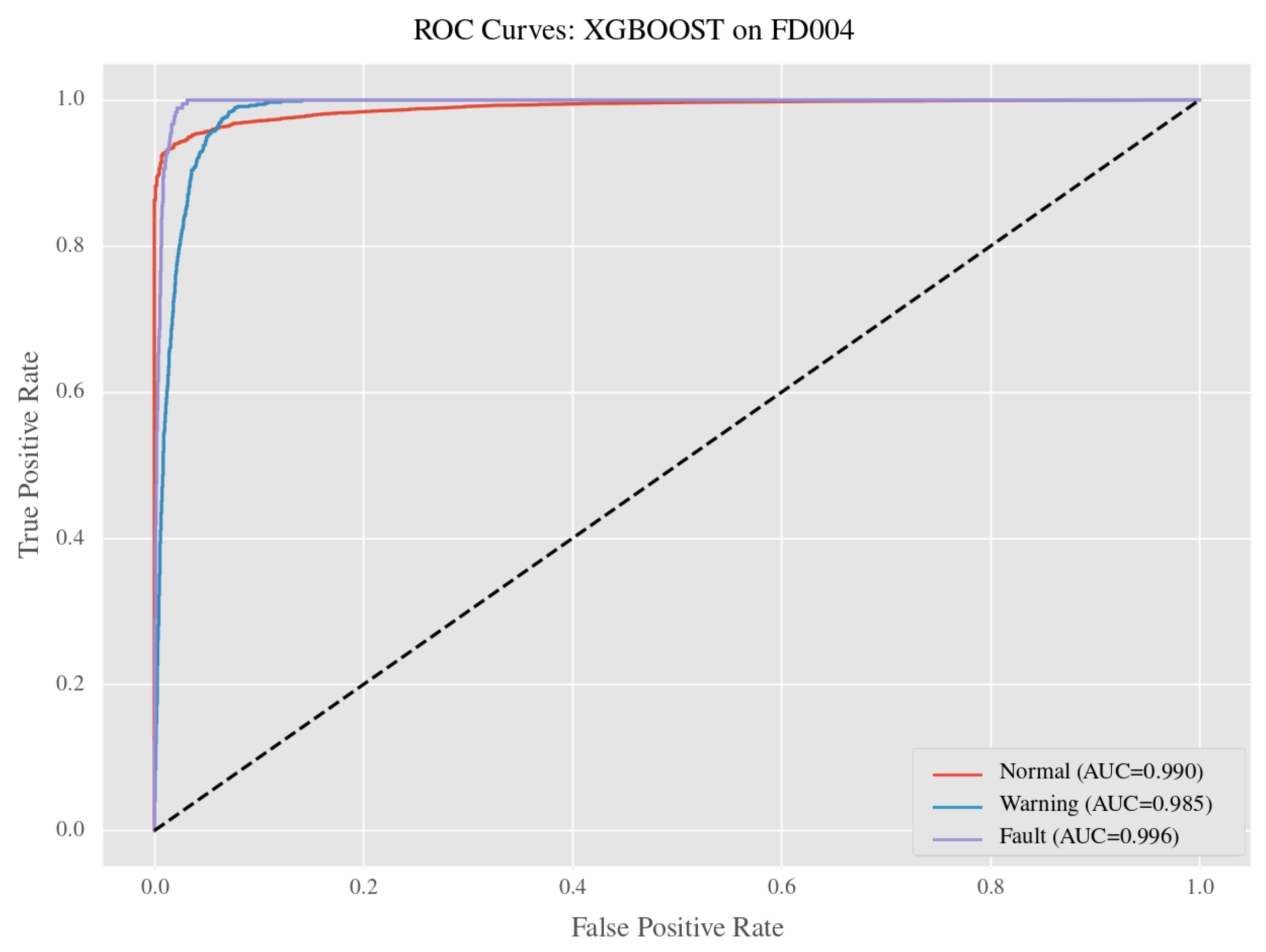
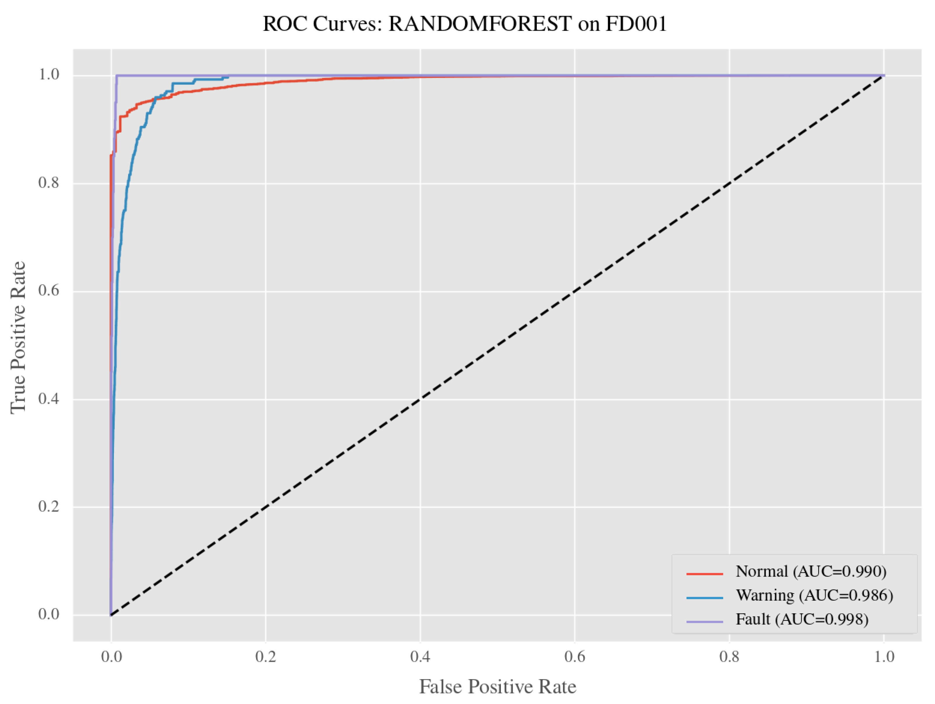
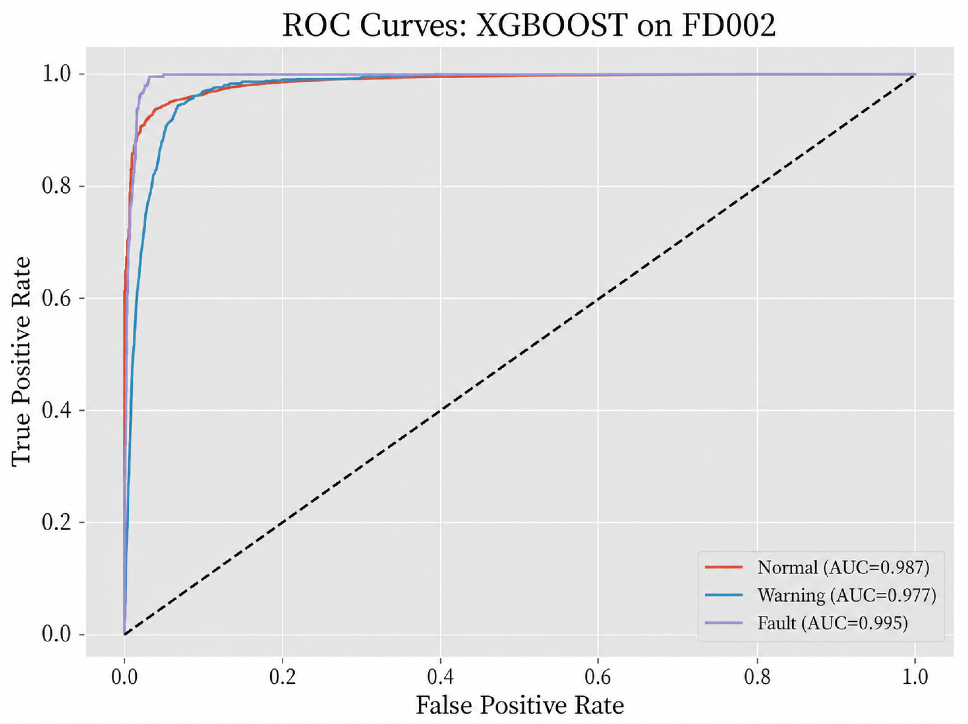
To further evaluate the class-wise discriminative ability of the proposed framework, the ROC curves of the best-performing model on each C-MAPSS subset are examined. Compared with hard-label metrics such as accuracy and F1-score, ROC analysis provides a more detailed view of how well the model separates different health states in the probability space. This is particularly important in the present study, because predictive maintenance not only requires correct classification outcomes, but also depends on reliable ranking behavior across Normal, Warning, and Fault states. The ROC results show that the best-performing models on FD001–FD004 achieve favorable discrimination performance, with curves remaining close to the upper-left region of the ROC space and class-wise AUC values at high levels across all subsets.
As shown in Figure 13, the ROC curves on FD001 show favorable class-wise separability for all three health states. The curves of the Normal and Fault classes remain close to the ideal upper-left boundary, indicating reliable discrimination under the single-condition setting. By contrast, the Warning class exhibits slightly weaker separation, which is consistent with the transitional nature of the intermediate degradation stage.
As shown in Figure 14, the ROC curves on FD002 indicate that the best-performing model maintains satisfactory discrimination ability under a more complex degradation environment. Compared with FD001, the Warning-class curve shows a slightly more inward shape, indicating reduced separability in the transitional state. This is consistent with the observation that multi-condition settings introduce additional distributional overlap near the decision boundary between healthy and degraded conditions.
Despite this increased difficulty, the Fault class retains favorable separability, with the corresponding ROC curve remaining close to the ideal boundary. This is important for predictive maintenance applications because it suggests that the model retains sensitivity to severe degradation even under more challenging operating conditions.
As shown in Figure 15, the ROC curves on FD003 show the most favorable overall discrimination performance among the four subsets, with all three class curves remaining close to the ideal upper-left region. This indicates that the learned representation achieves clearer class separation in FD003 relative to the other subsets under the present framework.
As shown in Figure 16, the ROC curves on FD004 also show good class-level separability, although the Warning class remains the least separable of the three categories. The Normal and Fault classes both show favorable ROC behavior, indicating that the framework distinguishes the two outer health states reasonably well even under a more complex operating scenario.
Compared with FD003, the ROC pattern of FD004 reveals slightly stronger overlap in the warning-related region, consistent with the increased heterogeneity of its degradation conditions. The intermediate health state continues to be the principal source of residual ambiguity, while the identification of fault-prone states remains comparatively reliable.
Overall, the ROC results indicate that the framework separates the two outer health states consistently across all subsets under the present benchmark conditions, while Warning-class discrimination remains the primary source of residual ambiguity. This pattern is consistent with the inherent difficulty of transitional degradation stages in aero-engine health evolution, and suggests that future improvements in intermediate-state characterization are likely to have the greatest practical impact.


4.6. Computational Cost Assessment

Table 9 reports the training time, total inference time, and per-window inference latency for all five evaluated models on the FD002 test partition, providing a preliminary deployment-oriented assessment of computational requirements. All per-window latency values are derived by dividing the total inference time by the number of test windows, and all measurements were obtained under the same local experimental environment.
LightGBM achieves the lowest per-window inference latency at 0.18 ms, followed by XGBoost at 0.31 ms and Random Forest at 0.42 ms, indicating that tree-based models are better suited for resource-aware or low-latency health-state monitoring. Bi-LSTM and MSTA-CNN require longer per-window inference times of 1.86 ms and 1.24 ms, respectively, owing to their sequential computation and deep feature extraction, but both remain at the millisecond level under the evaluated setting. These results indicate that the proposed framework is not prohibitively expensive for deployment in server-side monitoring environments, while tree-based models are the preferred choice when inference latency is a primary constraint.

4.7. Benchmark Positioning

Table 10 provides a qualitative positioning of the proposed framework relative to representative categories of recent C-MAPSS prognostics studies. A direct quantitative comparison is not presented because the task formulations differ fundamentally: most existing works optimize and report RMSE, NASA Score, or MAE for continuous RUL estimation under a fixed-piecewise target, whereas the present study reports Accuracy, Macro-F1, and class-wise F1 for discrete three-class health state classification. The proposed framework is therefore positioned as a complementary contribution rather than an incremental regression improvement.

5. Discussion and Conclusions

5.1. Main Findings

This study developed a condition-aware predictive maintenance framework for jet engines using the NASA C-MAPSS dataset. Instead of treating aero-engine degradation assessment as a conventional continuous remaining useful life prediction problem, the present work reformulated it as a three-class health state classification task involving Normal, Warning, and Fault states. This reformulation makes the prediction output more directly aligned with maintenance decision-making and improves the operational transparency of the final model output in practical engineering scenarios.
To support this maintenance-oriented task, a unified modeling pipeline was constructed. The framework integrates condition-wise normalization to reduce operating-condition bias, first-order differential feature construction to capture local degradation dynamics, and per-unit sliding window segmentation to preserve temporal continuity while avoiding cross-unit data leakage. On this basis, five representative models, including Random Forest, XGBoost, LightGBM, MSTA-CNN, and Bi-LSTM, were evaluated across the four C-MAPSS benchmark subsets FD001–FD004 under the same preprocessing and classification setting.
The experimental results demonstrate that the proposed framework achieves consistently high classification performance across all benchmark subsets. Tree-based models achieve the highest classification accuracy among the evaluated model families across all four subsets, indicating that the preprocessing pipeline transforms the original degradation sequences into a discriminative structured feature space that benefits ensemble methods. Among the deep learning models, Bi-LSTM consistently outperforms MSTA-CNN, which is consistent with the view that long-range temporal dependency is more informative than local pattern extraction for the present task. In addition, the confusion-matrix and ROC analyses show that the Normal and Fault classes are well separated, while the Warning state remains the most difficult category to distinguish because of its transitional nature.
Overall, the findings suggest that maintenance-oriented health state classification is a feasible and useful complement to conventional RUL-only modeling in a benchmark simulation setting. By combining condition-aware preprocessing, degradation-sensitive feature engineering, and comparative model evaluation within a unified framework, this study provides a methodological basis for exploring maintenance-decision-aligned alert generation under heterogeneous operating conditions, with direct applicability to real aero-engine systems subject to further validation. It should be noted that the interpretability discussed here refers to the operational transparency of the three-class output format, rather than to formal explainability analysis such as feature attribution or attention visualization, which is reserved for future work.

5.2. Discussion, Limitations, and Future Work

Several implications can be drawn from the present study. First, the consistently competitive performance of tree-based models in this benchmark suggests that carefully designed data representation plays an important role in maintenance-oriented health assessment. This is consistent with the observation that, for C-MAPSS-like degradation data, improved preprocessing and feature engineering may provide performance benefit comparable to that of more complex model architectures. Second, the advantage of Bi-LSTM over MSTA-CNN is consistent with the view that degradation progression is better characterized by long-term temporal evolution than by local temporal patterns alone, which aligns with the physically cumulative nature of aero-engine degradation. Third, the persistent difficulty of the Warning state highlights that intermediate degradation stages are intrinsically more ambiguous than the two outer states, which makes transitional-state modeling an important direction for future predictive maintenance research.
Despite these promising findings, several limitations should also be acknowledged. The first limitation lies in the task formulation itself. Although the three-class health state setting provides clearer operational meaning for maintenance decision support, the class boundaries still depend on the chosen label assignment strategy, and different state partition rules may lead to different classification behaviors. The second limitation is that the current study is conducted on a benchmark simulation dataset rather than real flight or maintenance records. Although C-MAPSS is valuable for methodological comparison, real-world engine data may contain additional noise, sensor drift, missing values, and operational uncertainty that are not fully represented in the benchmark environment. Translating the framework to real aero-engine systems would require additional steps such as sensor selection under physical constraints, handling of incomplete or asynchronous data streams, and domain adaptation to account for fleet-level variability. The third limitation concerns practical deployment feasibility. As reported in Table 9, tree-based models offer substantially lower per-window inference latency than neural network models, making them better suited for resource-constrained deployment. The proposed framework should be regarded as having potential for near-real-time maintenance decision support rather than being fully validated for onboard deployment; practical model selection should consider the trade-off among accuracy, latency, and computational resources according to the target scenario.
The fourth limitation is that explicit interpretability analysis, such as feature attribution methods or attention-weight visualization, has not been incorporated in the present study. The operational clarity gained from the three-class output format is a form of functional transparency but does not constitute formal explainability analysis. Integrating methods such as SHAP-based feature importance or gradient-weighted attention maps would strengthen the trustworthiness of the framework for maintenance operators and represents an important direction for future investigation.
As detailed in Table 10, the proposed framework is positioned as a complementary contribution to the dominant regression-based prognostic paradigm: rather than pursuing incremental improvements in continuous RUL estimation accuracy, it provides maintenance-decision-aligned discrete alert outputs that can be more directly integrated into operational maintenance scheduling.
Future research can be extended in several directions. One promising direction is to improve the modeling of the Warning state through threshold refinement, cost-sensitive learning, or class-aware calibration, so that early warning signals can be generated more reliably without reducing sensitivity to Fault states. A closely related direction is to incorporate uncertainty quantification methods—such as Bayesian deep learning, Monte Carlo dropout, or conformal prediction—to produce probabilistic confidence bounds for health state assignments, particularly in the transitional Warning region where classification confidence is inherently lower than for the two outer states. Such probabilistic outputs would enable maintenance operators to distinguish high-confidence Normal and Fault alerts from uncertain Warning-region assessments, thereby supporting risk-calibrated maintenance scheduling under operational ambiguity. Another direction is to integrate the current health state classification framework with continuous RUL estimation, thereby combining discrete maintenance alerts with finer-grained degradation quantification in a unified predictive maintenance system. In addition, future work should further investigate transferability and deployment robustness by evaluating the framework on real industrial datasets or under domain-shift conditions. More advanced sequence models and interpretable decision mechanisms could also be incorporated to strengthen practical applicability.

Author Contributions

Conceptualization, B.D. and C.Y.; methodology, B.D., C.Y., W.Z. and L.L.; software, L.H. and L.L.; validation, W.Z. and Y.F.; formal analysis, B.D. and X.Z.; investigation, L.H.; data curation, B.D.; writing—original draft preparation, B.D. and X.Z.; writing—review and editing, B.D. and X.Z.; visualization, X.Z.; project administration, C.Y.; funding acquisition, B.D., X.Z. and Y.F. All authors have read and agreed to the published version of the manuscript.

Funding

This research received no external funding.

Data Availability Statement

The C-MAPSS benchmark data used in this study are publicly available from the NASA Prognostics Center of Excellence. The processed sample matrices and label partitions are available on request from the corresponding author.

Acknowledgments

The authors are grateful to the reviewers for their constructive recommendations. Their perceptive questions and suggestions led to significant improvements in the methodological development and clarity of this work.

Conflicts of Interest

Author Weiyan Zhu was employed by the company Meta Platforms Inc. The remaining authors declare that the research was conducted in the absence of any commercial or financial relationships that could be construed as a potential conflict of interest.

Abbreviations

The following abbreviations are used in this manuscript:
CNNConvolutional Neural Network
MLPMultilayer Perceptron
RULRemaining Useful Life
STFTShort-Time Fourier Transform
RMSRoot Mean Square
PHMPrognostics and Health Management
MAEMean Absolute Error

Appendix A

The materials presented in Appendix A provide additional details on the dataset characteristics, preprocessing pipeline, and model configuration that support the empirical analyses reported in the main text. These materials are intended to improve reproducibility and provide a more complete reference for readers interested in implementation details.

Appendix A.1. Dataset Acquisition Parameters

Table A1 summarizes the main characteristics of the four C-MAPSS benchmark subsets evaluated in this study.
Table A1. Key characteristics of the C-MAPSS subsets used for model evaluation.
SubsetOperating ConditionsFault ModesTraining UnitsTest Units
FD001SingleSingle100100
FD002MultipleSingle260259
FD003SingleMultiple100100
FD004MultipleMultiple249248

Appendix A.2. Feature Extraction Summary

The 783-dimensional handcrafted feature vector used in the MLP branch is organized into distinct categories. Table A2 summarizes the category dimension allocation and the approximate contribution of each category to the final feature importance ranking obtained from the trained model.
Table A2. Quantitative summary of handcrafted feature categories and their relative importance contribution.
CategoryFeature CountDimension RatioEstimated Importance Share
Time-domain statistics202.6%14.2%
Frequency-domain features303.8%18.7%
Envelope statistics202.6%9.5%
Autocorrelation features506.4%11.9%
Entropy measures151.9%7.3%
Wavelet coefficients20025.5%21.8%
STFT-derived features40051.1%14.9%
Other descriptors486.1%1.7%

Appendix A.3. Post-Processing Sample Distribution

Table A3 reports the window-level health state distribution obtained after condition-wise normalization, first-order differential feature construction, and per-unit sliding window segmentation. These values illustrate the class composition that the classifiers are trained on and highlight the relative imbalance among the Normal, Warning, and Fault alerts.
Table A3. Window-level health state distribution after preprocessing for each C-MAPSS subset.
SubsetNormalWarningFaultTotal Windows
FD00138,40011,200580055,400
FD002110,60018,90011,700141,200
FD00340,80013,000690060,700
FD004119,50024,10015,400159,000

References

  1. Lee, J.; Mitici, M. Deep reinforcement learning for predictive aircraft maintenance using probabilistic remaining-useful-life prognostics. Reliab. Eng. Syst. Saf. 2022, 230, 108908. [Google Scholar]
  2. Xue, F.; Jin, G.; Tan, L.; Zhang, C.; Yu, Y. Predictive maintenance programs for aircraft engines based on remaining useful life prediction. Sci. Rep. 2025, 15, 19957. [Google Scholar] [CrossRef] [PubMed]
  3. Pater, I.; Reijns, A.; Mitici, M. Alarm-based predictive maintenance scheduling for aircraft engines with imperfect remaining useful life prognostics. Reliab. Eng. Syst. Saf. 2022, 221, 108341. [Google Scholar] [CrossRef]
  4. Elsherif, S.; Hafiz, B.; Makhlouf, M.; Farouk, O. A deep learning-based prognostic approach for predicting turbofan engine degradation and remaining useful life. Sci. Rep. 2025, 15, 9155. [Google Scholar] [CrossRef] [PubMed]
  5. Xiong, M.; Wang, H.; Fu, Q.; Xu, Y. Digital twin-driven aero-engine intelligent predictive maintenance. Int. J. Adv. Manuf. Technol. 2021, 114, 3751–3761. [Google Scholar] [CrossRef]
  6. Wang, L.; Chen, Y.; Zhao, X.; Xiang, J. Predictive maintenance scheduling for aircraft engines based on remaining useful life prediction. IEEE Internet Things J. 2024, 11, 23020–23031. [Google Scholar] [CrossRef]
  7. Zhou, M.; Miao, K.; Sun, J.; Shen, Y.; Han, B. Data-driven modeling of aero-engine performance degradation models. IEEE Access 2024, 12, 150020–150031. [Google Scholar]
  8. Mitici, M.; Pater, I.; Barros, A.; Zeng, Z. Dynamic predictive maintenance for multiple components using data-driven probabilistic RUL prognostics: The case of turbofan engines. Reliab. Eng. Syst. Saf. 2023, 234, 109199. [Google Scholar] [CrossRef]
  9. Wang, C.; Zhu, Z.; Lu, N.; Cheng, Y.; Jiang, B. A data-driven degradation prognostic strategy for aero-engine under various operational conditions. Neurocomputing 2021, 462, 195–207. [Google Scholar]
  10. Wang, C.; Lu, N.; Cheng, Y.; Jiang, B. A data-driven aero-engine degradation prognostic strategy. IEEE Trans. Cybern. 2019, 51, 1531–1541. [Google Scholar]
  11. Rath, N.; Mishra, R.; Kushari, A. Aero engine health monitoring, diagnostics and prognostics for condition-based maintenance: An overview. Int. J. Turbo Jet-Engines 2022, 40, s279–s292. [Google Scholar] [CrossRef]
  12. Chen, C.; Shi, J.; Lu, N.; Zhu, Z.; Jiang, B. Data-driven predictive maintenance strategy considering the uncertainty in remaining useful life prediction. Neurocomputing 2022, 494, 79–88. [Google Scholar] [CrossRef]
  13. De Giorgi, M.; Menga, N.; Ficarella, A. Exploring prognostic and diagnostic techniques for jet engine health monitoring: A review of degradation mechanisms and advanced prediction strategies. Energies 2023, 16, 2711. [Google Scholar] [CrossRef]
  14. Khan, K.; Sohaib, M.; Rashid, A.; Ali, S.; Akbar, H.; Basit, A.; Ahmad, T. Recent trends and challenges in predictive maintenance of aircraft’s engine and hydraulic system. J. Braz. Soc. Mech. Sci. Eng. 2021, 43, 487. [Google Scholar] [CrossRef]
  15. Srivatsa, A.; Goudar, V.; Naveen, T.; Peri, R.; Banik, D.; Kumar, R. Physics-informed machine learning for predicting remaining useful life of aircraft engines: A robust framework for risk-aware maintenance. In Proceedings of the 2025 IEEE International Conference on Emerging Technologies and Applications (MPSec ICETA), Bengaluru, India, 22–23 May 2025; IEEE: New York, NY, USA, 2025; pp. 1–6. [Google Scholar]
  16. J, D.; Reddy, P.; Murari, K.; Rahul, B. Predictive maintenance of aircraft engines: Machine learning approaches for remaining useful life estimation. In Proceedings of the 2025 6th International Conference on Mobile Computing and Sustainable Informatics (ICMCSI), Lalitpur, Nepal, 7–8 March 2025; IEEE: New York, NY, USA, 2025; pp. 1679–1686. [Google Scholar]
  17. Fu, S.; Avdelidis, N. Prognostic and health management of critical aircraft systems and components: An overview. Sensors 2023, 23, 8124. [Google Scholar] [CrossRef] [PubMed]
  18. Zhu, Z.; Wang, L.; Chen, M.; Zhao, X. Predictive maintenance strategies for aero-engines considering remaining useful life prediction interval. Qual. Reliab. Eng. Int. 2025, 41, 3350–3359. [Google Scholar] [CrossRef]
  19. Özcan, H. Interpretable ensemble remaining useful life prediction enables dynamic maintenance scheduling for aircraft engines. Sci. Rep. 2025, 15, 23473. [Google Scholar] [CrossRef] [PubMed]
Figure 1. Distribution of total engine lifetime in the training subset FD001.
Machines 14 00695 g001
Figure 2. Representative degradation trends of selected informative sensors from an engine unit.
Machines 14 00695 g002
Figure 3. Leakage-free data splitting and preprocessing workflow.
Machines 14 00695 g003
Figure 4. Standardized distributions and outlier patterns of selected sensor channels.
Machines 14 00695 g004
Figure 5. Correlation matrix of selected informative sensors.
Machines 14 00695 g005
Figure 6. Accuracy comparison of five models across FD001–FD004.
Machines 14 00695 g006
Figure 7. F1-score comparison of five models across FD001–FD004.
Machines 14 00695 g007
Figure 8. Overall benchmark comparison across all models and datasets.
Machines 14 00695 g008
Figure 9. Confusion matrix of the best-performing model on FD001.
Machines 14 00695 g009
Figure 10. Confusion matrix of the best-performing model on FD002.
Machines 14 00695 g010
Figure 11. Confusion matrix of the best-performing model on FD003.
Machines 14 00695 g011
Figure 12. Confusion matrix of the best-performing model on FD004.
Machines 14 00695 g012
Figure 13. ROC curves of the best-performing model on FD001.
Machines 14 00695 g013
Figure 14. ROC curves of the best-performing model on FD002.
Machines 14 00695 g014
Figure 15. ROC curves of the best-performing model on FD003.
Machines 14 00695 g015
Figure 16. ROC curves of the best-performing model on FD004.
Machines 14 00695 g016
Table 1. Positioning against representative studies on aero-engine predictive maintenance and prognostics (qualitative comparison).
Study (Ref.)Degradation/RUL PrognosticsMaintenance Scheduling/Program DesignUncertainty/Risk AwarenessAdvanced Learning FrameworkInterpretability/
Engineering Transparency
Integrated Decision Support
Data-driven prognostic studies [7,9,10]partialpartial
Deep-learning-based prognostic studies [4,15,16]partialpartialpartialpartial
RUL-oriented maintenance strategy studies [3,6,8,12,18]partialpartial
Scheduling-oriented decision studies [1,2,3,8,19]partialpartialpartial
Digital-twin/PHM framework and review studies [5,11,13,14,17]partialpartialpartialpartialpartial
This work(integrated aero-engine prognostics)(maintenance-oriented modeling objective)(uncertainty-aware maintenance perspective)(advanced data-driven learning framework)(maintenance-decision-oriented and engineering-relevant analysis)(unified prognosis-to-maintenance support)
Bold entries denote the proposed framework (this work).
Table 2. Definition of health-state labels based on RUL thresholds.
Health StateLabelRUL Range (Cycles)Maintenance Interpretation
Normal0RUL > 80The engine operates in a relatively healthy state, and no immediate maintenance action is required.
Warning130 < RUL ≤ 80Observable degradation has appeared, and maintenance attention or inspection should be scheduled.
Fault2RUL ≤ 30The engine is approaching the failure stage, and maintenance intervention is required with high priority.
Table 3. Label distribution across FD subsets under the baseline health-state definition (window-level sample counts).
FD SubsetNormalWarningFaultTotal Windows
FD0019842 (47.68%)6421 (31.11%)4377 (21.21%)20,640
FD00225,316 (49.23%)15,814 (30.75%)10,292 (20.02%)51,422
FD00311,284 (48.56%)7043 (30.31%)4910 (21.13%)23,237
FD00429,876 (49.87%)18,126 (30.25%)11,908 (19.88%)59,910
Table 4. Sensitivity analysis of health-state threshold selection (XGBoost on FD002).
Threshold SettingNW/WF (Cycles)AccuracyMacro-F1Normal F1Warning F1Fault F1
Conservative90/400.97310.96840.97950.95310.9726
Baseline80/300.97640.97120.98310.95630.9742
Aggressive70/200.97120.96680.97860.94980.9720
Table 5. Statistical stability of neural network models over five repeated runs (FD002 validation partition, mean ± standard deviation; 95% CI of Macro-F1 estimated using the t-distribution with 4 degrees of freedom).
ModelRunsAccuracyPrecisionRecallMacro-F195% CI (Macro-F1)
Bi-LSTM5 0.963 ± 0.003 0.961 ± 0.004 0.959 ± 0.003 0.954 ± 0.004 [0.949, 0.959]
MSTA-CNN5 0.964 ± 0.002 0.961 ± 0.003 0.958 ± 0.003 0.956 ± 0.003 [0.952, 0.960]
Table 6. Classification accuracy of different models on the four C-MAPSS subsets.
DatasetXGBoostLightGBMRandom ForestMSTA-CNNBi-LSTM
FD0010.98350.98340.98410.97390.9804
FD0020.97640.97570.97560.96140.9747
FD0030.98870.98910.98840.98430.9876
FD0040.98320.98270.98260.97730.9806
Table 7. Performance summary of the MSTA-CNN model on the four C-MAPSS subsets. All metrics are weighted-average values computed on the designated test partition under the same evaluation protocol as Table 6.
DatasetAccuracyPrecisionRecallF1-Score
FD0010.97390.97530.97390.9746
FD0020.96140.96630.96140.9638
FD0030.98430.98380.98430.9840
FD0040.97730.97670.97730.9770
Table 8. Ablation study of preprocessing and temporal modeling components (Bi-LSTM on FD002 validation split).
VariantCond. Norm.Diff. FeaturesSliding WindowTemporal ModelingAccuracyMacro-F1Warning F1Fault F1
Full framework0.96400.95600.94400.9550
Variant A×0.95100.94100.92300.9430
Variant B×0.95600.94800.93400.9460
Variant C×0.94800.93900.92100.9400
Variant D×0.95700.94900.93500.9470
Variant E××××0.93500.92600.90500.9200
✓: component included; ×: component removed.
Table 9. Computational cost and deployment-related characteristics of candidate models (FD002 test partition).
ModelTraining Time (s)Total Inference Time (s)Per-Window Latency (ms)Resource DemandDeployment Implication
Random Forest38.66.300.42MediumSuitable for offline diagnosis and server-side batch inference
XGBoost52.44.650.31MediumSuitable for efficient online inference after model training
LightGBM29.82.700.18Low–mediumFavorable for resource-aware deployment with low latency
Bi-LSTM214.727.901.86HighRequires sequential computation; more suitable for server-side or
GPU-assisted monitoring
MSTA-CNN176.318.601.24Medium–highSuitable for near-real-time inference with GPU or edge-accelerator support
The inference time per window was calculated by dividing the total inference time by the number of test windows in the FD002 test partition. All computational costs were measured under the same local experimental environment.
Table 10. Qualitative positioning of the proposed framework relative to representative categories of recent C-MAPSS prognostics studies.
Study CategoryDatasetMain TechniqueTask FormulationOutputEval. MetricRelation to This Work
Transformer-based prognosticsC-MAPSS FD001–FD004Self-attention encoder; multi-head temporal attentionRUL regressionContinuous RULRMSE/ScoreStrong global temporal modeling; output is a numerical life estimate, not a discrete maintenance alert
Hybrid Transformer/recurrent modelsC-MAPSS FD001–FD004Transformer combined with BiLSTM, CNN, or nonlinear mapping modulesRUL regressionContinuous RULRMSE/Score/
MAE
Higher representation capacity; typically more complex architectures targeting regression accuracy
Spatio-temporal graph modelsC-MAPSS FD001–FD004GNN/temporal
sensor graph
RUL regressionContinuous RULRMSE/ScoreExplicit inter-sensor dependency modeling; this work uses preprocessing-driven feature representation with simpler relational structure
Domain adaptation prognosticsCross-condition or cross-dataset C-MAPSSTransfer learning; adversarial adaptation; domain-invariant representationRUL regression or health indicator learningContinuous RUL/HIRMSE/transfer metricFocuses on source-to-target distribution shift; this work evaluates all FD subsets under a unified in-domain protocol
Uncertainty-aware prognosticsC-MAPSS FD001–FD004Bayesian inference; MC dropout; evidential regressionProbabilistic RUL estimationRUL distribution/confidence intervalRMSE/coverage/
calibration
Provides confidence-aware output; this work focuses on deterministic three-class health state classification
Proposed frameworkC-MAPSS FD001–FD004Condition-aware preprocessing + differential features + sliding windows + ML/DL classifiersMulti-class health-state classificationNormal/Warning/Fault labelsAccuracy/Macro-F1/class-wise F1Provides direct maintenance-oriented discrete alert outputs; complements regression-based methods rather than replacing them
Bold entries denote the proposed framework (this work).
Disclaimer/Publisher’s Note: The statements, opinions and data contained in all publications are solely those of the individual author(s) and contributor(s) and not of MDPI and/or the editor(s). MDPI and/or the editor(s) disclaim responsibility for any injury to people or property resulting from any ideas, methods, instructions or products referred to in the content.