Article

Bearing Dynamics Identification with SINDy-Based Neural Network and Physics Model

1
Dongfang Turbine Co., Ltd., Deyang 618000, China
2
School of Aeronautics and Astronautics, Zhejiang University, Hangzhou 310027, China
3
School of Rail Transit, Zhejiang Institute of Communications, Hangzhou 311112, China
4
Marine Department, Zhejiang Institute of Communications, Hangzhou 311112, China
*
Author to whom correspondence should be addressed.
These authors contributed equally to this work.
Machines 2026, 14(6), 620; https://doi.org/10.3390/machines14060620
Submission received: 28 April 2026 / Revised: 26 May 2026 / Accepted: 27 May 2026 / Published: 29 May 2026

Abstract

Deep neural networks can fit nonlinear bearing vibration responses, but their learned parameters are difficult to relate to contact deformation, rolling element angular position, and other acceleration-generating mechanisms. To improve physical traceability in data-driven bearing dynamics identification, this study develops a physics-informed SINDy-NN with a mechanism-guided feature library. This paper presents a novel approach for constructing a physics-informed SINDy-NN (Sparse Identification of Nonlinear Dynamics-based Neural Network) and demonstrates its application in identifying bearing dynamics. A 5-DoF (five Degrees of Freedom) bearing dynamics model is built, and the primary components influencing the acceleration response are analyzed. This analysis forms the basis for defining a physics-explainable basis function library for the SINDy-NN. For comparison, widely used polynomial and Fourier libraries are also employed to evaluate modeling accuracy and convergence speed. Furthermore, to address the limited number of bearing data, virtual states are generated by applying multiple finite differences to the acceleration signal, expanding the dimensionality of the model and enabling the use of a Multi-Input–Multi-Output (MIMO) model in SINDy-NN. Finally, experimental data from the FEMTO bearing test bench are utilized for validation. The results demonstrate that the physics-informed SINDy-NN offers superior modeling efficiency, with sufficient accuracy and improved interpretability compared to general SINDy-NN.

1. Introduction

As a critical component in rotating machinery, the health of bearings significantly affects equipment service life. Dynamic modeling and identification are essential for analyzing bearing responses under various conditions [1], providing critical insights for monitoring and fault diagnosis [2]. Currently, there are two primary approaches to bearing dynamics modeling: model-based and data-driven methods.
The model-based approach simulates bearing dynamics based on physical principles. For example, kinetic models grounded in Hertzian contact theory and the finite element method have been effective in detecting defects in angular contact ball bearings [3,4,5]. Additionally, several studies have focused on modeling the vibration response of faulty bearings. Cui et al. [6] developed a nonlinear vibration model for a 5-DoF rolling bearing by integrating Hertzian contact theory with a single-point local failure model. Further research [7] extended the 5-DoF model, incorporating more complex multi-body dynamics and contact mechanics. Model-based methods generally rely on accurate physical parameters, but uncertainties and computational instabilities can arise when dealing with nonlinear or complex models [8]. Moreover, high-precision models often require extensive parameter identification, leading to increased computational time [9]. To address these challenges, some researchers have explored simplified dynamic modeling techniques, such as SINDy and Hammerstein–Wiener models [10]. Kaheman et al. [11] used Parallel Implicit Sparse Identification of Nonlinear Dynamics (SINDy-PI) to identify a range of Open Dynamics Engine (ODE) and Partial Differential Equation (PDE) dynamics, including the double pendulum and the Belousov–Zhabotinsky (BZ) reaction. Similarly, Omar et al. [12] proposed a framework combining the SINDy-PI algorithm with the Akaike Information Criterion (AIC) to extract dynamic equations for serial manipulators, while Arora et al. [13] employed model-based reinforcement learning with SINDy to discover and generalize physics-based dynamic systems. Lenfesty et al. [14] demonstrated the effectiveness of SINDy in modeling systems with accelerating dynamical components during decision formation.
Data-driven models have been widely used to estimate bearing degradation states and vibration responses when exact contact parameters or system-level dynamic parameters are difficult to obtain [15]. Koca et al. proposed a VMD-Transformer-rCCA framework for bearing fault classification, where variational mode decomposition is used for noise suppression, Transformer networks extract deep representations, and regularized canonical correlation analysis enhances feature fusion [16]. Liu et al. [17] proposed the Dynamic Latent Variable Reconstruction Nonlinear Wiener Process (DLVR-NWP), where dynamic features relevant to bearing degradation are extracted for accurate estimation of Remaining Useful Life (RUL). Zhao et al. [18] developed a Nonlinear Auto-Regressive with Exogenous inputs (NARX) model, which combined nonlinear output frequency response functions to assess the impact of friction on bearing-rotor systems quantitatively. Babin et al. [19] demonstrated that nonlinear fluid-film bearing identification using artificial neural networks improves the efficiency of simulation models and control system design. Unlike model-based approaches, data-driven methods do not require prior knowledge of the system, although they often necessitate large amounts of data for training [20]. To mitigate data scarcity, existing studies have explored data augmentation [21], virtual sample generation [22], and transfer learning [23]. For example, Ge et al. proposed a broad learning system with virtual sample generation (BLS-VSG) for CFRP drilling performance prediction, in which virtual samples were generated to improve prediction performance under limited experimental data [22]. These studies show that enlarging or enriching the training data can be an effective way to improve data-driven modeling when real experimental samples are limited. Moreover, data-driven models frequently involve complex network architectures with parameters far exceeding the original system’s dimensions, and deep learning hyperparameter optimization often lacks mechanistic interpretability [24].
To improve the interpretability of black-box neural networks, recent studies have incorporated physical knowledge into network design. Ruan et al. proposed a deep stacked state-observer-based neural network (DSSO-NN), where state-space equations and state-observer structures are embedded for system dynamics modeling and bearing applications [25]. Wu et al. developed a physics-guided interpretable Inception network for bearing fault diagnosis, in which the input length, convolution kernel size, and branch structure are designed according to bearing vibration characteristics, including fault characteristic frequency, shaft rotation frequency, and single-period acceleration responses [26]. These studies indicate that physical knowledge can improve not only model performance but also the traceability of learned representations to bearing mechanisms.
Following this trend, this study explores interpretability at the feature-library level of SINDy-NN. Unlike approaches that mainly embed physical knowledge into network architecture or parameter design, this work converts simplified bearing contact relationships into candidate basis functions for sparse dynamics identification. To address these limitations, this study develops a physics-informed SINDy-NN for bearing dynamics identification by embedding simplified contact-force relationships from a 5-DoF bearing model into the candidate feature library. Specifically, the measured acceleration components are analyzed from the kinematic differential equations of the 5-DoF bearing model, and the relationships among contact deformation, rolling element angular position, and acceleration response are derived. Based on this simplified mechanism, a physically traceable sparse feature library is constructed, allowing selected basis functions to be linked to the main acceleration-generating mechanisms of the bearing.
The novelty of this work lies in the construction of a bearing-specific SINDy-NN feature library for acceleration dynamics identification, rather than in the use of SINDy-NN alone. Different from generic libraries based on standard polynomial or Fourier terms, the proposed library is derived from the vertical contact-force relationship of the 5-DoF bearing model. Polynomial-type terms are associated with Hertzian contact deformation, while trigonometric terms are associated with rolling element angular position. Therefore, the identified SINDy terms can be traced to specific acceleration-generating mechanisms in the bearing.
The primary contributions of this work are summarized as follows:
  • A bearing-specific feature-library construction method is proposed for SINDy-NN-based bearing dynamics identification. The library is derived from the vertical contact-force relationship of the 5-DoF bearing model, where polynomial-type terms are associated with Hertzian contact deformation and trigonometric terms are associated with rolling element angular position. This design improves the physical traceability of the identified SINDy terms compared with generic polynomial or Fourier libraries.
  • A finite-difference-based virtual-state strategy is introduced to extend limited measurable acceleration data into a Multi-Input–Multi-Output (MIMO) state representation. Unlike sample-level data augmentation, this strategy enriches the dynamic state description without generating artificial bearing samples, enabling SINDy-NN to identify bearing dynamics under limited measurable-state conditions.
  • A systematic comparison among standard polynomial, Fourier, and custom feature libraries is conducted to evaluate the proposed library. The results show that the mechanism-guided custom library achieves a favorable balance among modeling accuracy, training time, and physical traceability with fewer candidate functions.
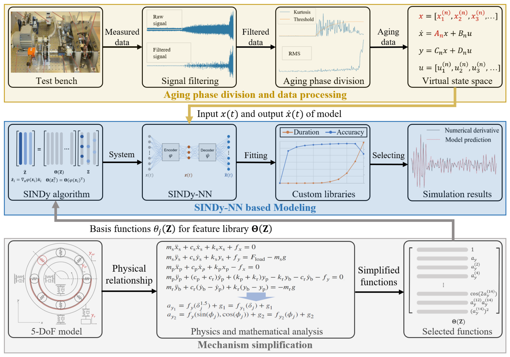
Figure 1 presents the overall structure of this study, divided into three main components: aging phase division and data processing, mechanism simplification, and SINDy-NN-based modeling. The first section focuses on methods for obtaining higher-quality signals and selecting valid data. Mechanism simplification allows physical knowledge to be embedded into neural networks. Finally, the modeling section demonstrates the advantages of the SINDy-NN, leveraging the mechanism-based feature library to improve modeling efficiency. The remainder of this paper is organized as follows: Section 2 introduces the SINDy-NN and the bearing dynamics model. Section 3 discusses the database, test platform, and data preprocessing, including methods for filtering signals and dividing the bearing aging phase. Section 4 presents experiments and analyzes standard libraries. Section 5 focuses on constructing the custom library based on experimental results, and Section 6 concludes the study and discusses avenues for future research.

2. Background Theory

2.1. SINDy-Based Neural Network (SINDy-NN)

SINDy-NN is a custom deep autoencoder network with sparse regression in a library of candidate terms to obtain a parsimonious model [27,28], which allows us to integrate a simple mechanism into data-driven modeling. By combining the model’s governing equations with the coordinate system, SINDy can discover effective coordinate transformations and use the fewest terms to quickly identify the structure and parameters of nonlinear dynamic systems from data [29]. Take the system in Equation (1) as an example; the SINDy-based modeling is to discover a best-fit dynamic system constrained by the sparse function f with as few active terms as possible [30]:
d d t x t = f x t .
Suppose a complex physical model can be represented by a parsimonious model that is sparse based on possible functions. Model discovery can be framed as a sparse regression problem. Derivatives from x ( t ) can be used to form data matrices X = [ x 1 x 2 x m ] T and X ˙ = [ x ˙ 1 x ˙ 2 x ˙ m ] T , with X , X ˙ R m × n . An extensive feature library of p candidate functions Θ X = [ θ 1 X θ 2 X θ p X ] R m × p can be constructed to formulate an overdetermined linear system:
X ˙ = Θ X Ξ ,
where each θ j X ( j = 1 , 2 , , p ) is a candidate model term, and the matrix Ξ = [ ξ 1 ξ 2 ξ n ] R p × n is the set of coefficients that determine the active terms in Θ X . The SINDy approach with a sequentially thresholded least-squares algorithm is used to solve the coefficient matrix Ξ , which is a proxy for l 0 optimization and has convergence guarantees, ensuring that only a few columns of Θ X are selected [31,32]. For high-dimension systems, it uses the dynamics z ˙ = g z to seek a set of reduced coordinates z t = φ x t R d ( d n ) , as shown in Equation (3) [30].
d d t z t = g z t = Θ z t Ξ .
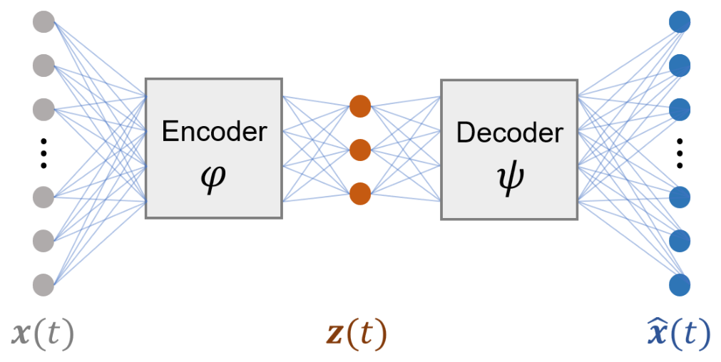
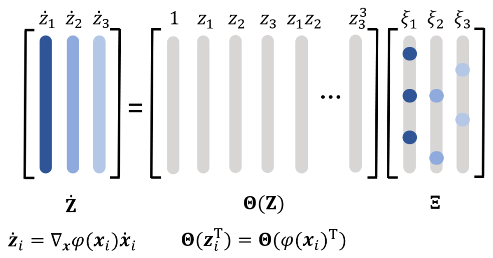
SINDy-NN is implemented through the autoencode structure, as shown in Figure 2. The autoencoder has a simple structure and excellent feature extraction and data reconstruction capabilities, enabling it to achieve better dimensionality reduction and capture nonlinearity. This feedforward neural network has an encoder φ x , a decoder ψ z , and a hidden layer representing the intrinsic coordinates z t . It learns the coordinates associated with a simple mechanism by simultaneously learning a dynamic SINDy model from high-dimensional input measurement data x , ensuring the sparse dynamics models associated with intrinsic coordinates. The regularization is achieved by constructing a library Θ z of candidate basis functions θ j z , e.g., polynomials, and learning Ξ that defines the dynamic system in Equation (3). Figure 3 shows a SINDy model that captures the dynamics of the intrinsic coordinates. The active terms are identified by the nonzero elements in the sparse matrix Ξ , which are learned with the neural network parameters as part of the training procedure. The time derivatives of z t are calculated using the derivatives of x t and the gradient of the encoder φ x [30].
SINDy-NN needs a pointwise loss function to train the network and minimize the autoencoder reconstruction error and the total loss L loss of SINDy, including the reconstruction loss termed as L recon , SINDy loss in x ˙ t termed as L d x / d t , SINDy loss in z ˙ t termed as L d z / d t , and an L 1 regularization termed as L reg [30]:
L loss = L recon + λ 1 L d x / d t + λ 2 L d z / d t + λ 3 L reg ,
where the hyperparameters λ 1 , λ 2 , and λ 3 determine the relative weights and are defined using the Adam optimizer during training [33]. The time derivatives of the raw data x ( t ) can be reconstructed by SINDy with the Equation (5):
L d x / d t = x ˙ z ψ φ x Θ φ x T Ξ 2 2 .
The derivative of the variables z ( t ) can enforce accurate prediction of the dynamics with the term in Equation (6):
L d z / d t = x φ x x ˙ Θ φ x T Ξ 2 2 .
Equation (7) gives the standard autoencoder loss:
L recon = x ψ φ x 2 2 ,
which ensures that the autoencoder can accurately reconstruct the input data. The L 1 regularization L reg of SINDy coefficients Ξ promotes the coefficients’ sparsity and brings a simple dynamics model. Upon analysis, it becomes evident that the SINDy-NN leverages the strengths of Deep Neural Networks (DNNs) for flexible representation and SINDy for sparse modeling with basis functions [30]. Different basis functions represent distinct dynamic components for modeling. Existing research underscores the pivotal role of the defined feature library in influencing the performance of SINDy-NN [34]. Many previously published studies adopted the default feature library, such as polynomial functions [35]. Although some recent studies have explored diverse feature libraries, these alternatives fall short in elucidating the intricacies of system dynamics [11,34]. The few explorations of SINDy custom libraries are limited to some uncomplicated model mechanisms. Theoretically, deriving the feature library from the system physics model is posited to enhance the accuracy, convergence speed, and interpretability of SINDy-NN. To experimentally validate this hypothesis, this study explores constructing the feature library for SINDy-NN by analyzing the 5-DoF bearing dynamics model.

2.2. Bearing Mechanism

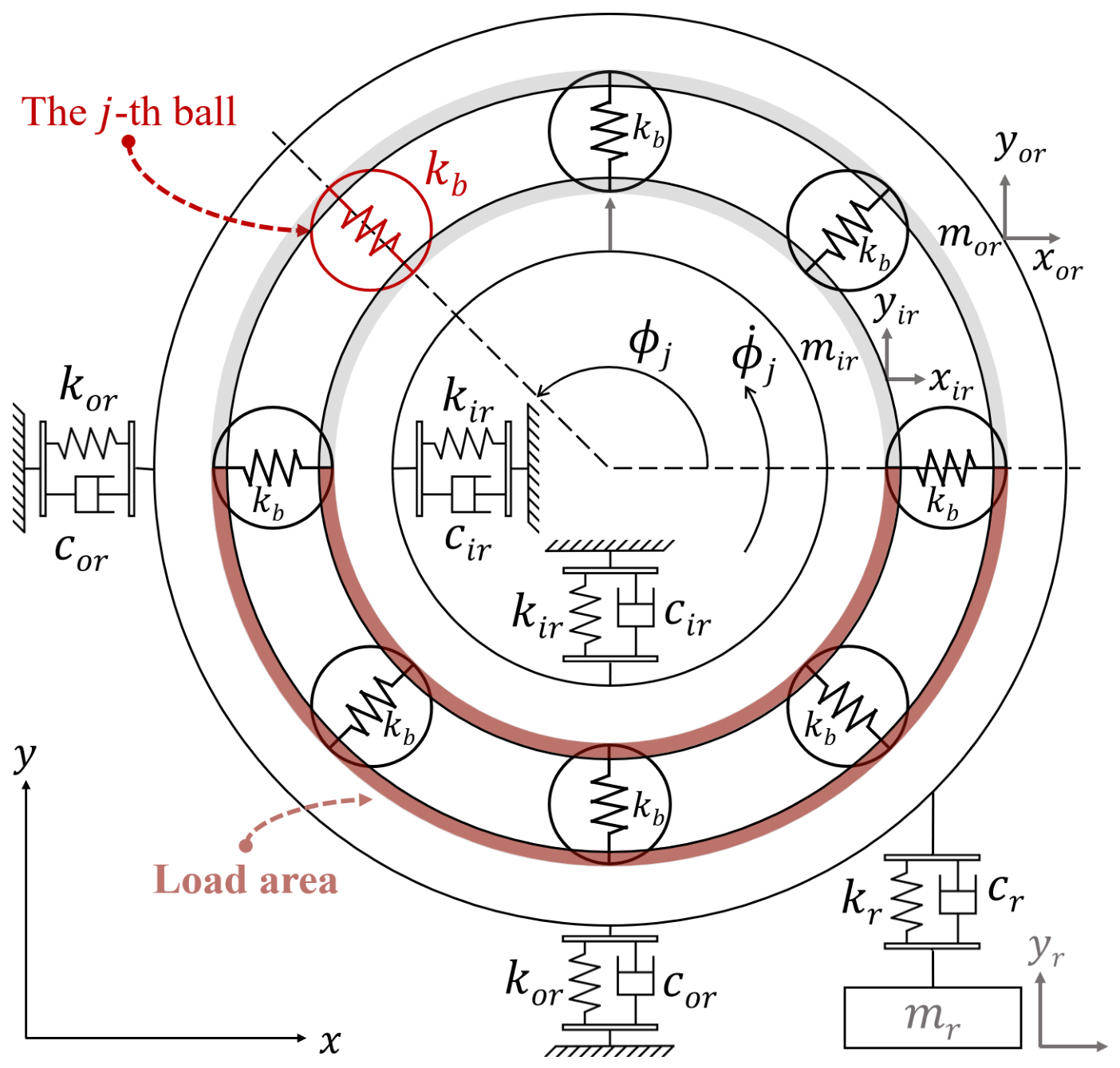
In this study, the physics-informed SINDy-NN will be implemented by extracting the simple mechanism from physics models, and bearing is taken as the research object. As shown in Figure 4, a 5-DoF model is built to identify the bearing dynamics and can be presented by Equations (8)–(13) [6]:
m s x ¨ s + c s x ˙ s + k s x s + f x = 0 ,
m s y ¨ s + c s y ˙ s + k s y s + f y = F load m s g ,
m p x ¨ p + c p x ˙ p + k p x p f x = 0 ,
m p y ¨ p + ( c p + c r ) y ˙ p + ( k p + k r ) y p k r y b
c r y ˙ b f y = 0 ,
m r y ¨ b + c r ( y ˙ b y ˙ p ) + k r ( y b y p ) = m r g ,
where m s , m p , m r , respectively, represent the mass of the inner race, outer race, and unit resonators; k s , k p , k r , respectively, represent the stiffness of the inner race, outer race, and unit resonators; c s , c p , c r , respectively, represent the damping of the inner race, outer race, and unit resonators; f x , f y , respectively, represent the nonlinear contact force of the bearing in the horizontal direction and vertical direction; x s , y s , x p , y p , y b , respectively, mean the two inner race DoF, two outer race DoF, and measured vibration response. g is the gravitational acceleration. F load is the vertical external force applied to the inner race of the bearing. The detailed mathematical model can be referred to in the research in reference [36].
The lumped parameter method simplifies the system by treating all balls as a single entity. The contact force f j between the j-th ball and the raceway is split into horizontal ( f x j ) and vertical ( f y j ) components. Focusing on the vertical vibration signal, the relationship between vertical acceleration a y and vertical contact force f y is established through Newton’s second law, given by Equation (14) [10]:
a y = f y m = j = 1 n b f y j j = 1 n b m j ,
where n b denotes the number of balls in the bearing and m j the mass of the j-th ball. From the Hertzian contact theory, the contact force f j between the j-th ball and the raceway is given by Equation (15):
f j = k b δ j 1.5 .
The total nonlinear contact force of bearing in the y-direction is calculated by Equation (16):
f y = j = 1 n b f y j = k b j = 1 n b γ j δ j 1.5 sin ϕ j ,
where γ j is a switch function. The ball is deformed only when located in the load zone; thus, the contact force is produced. γ j is determined in Equation (17) [6]:
γ j = 1 , δ j > 0 , 0 , otherweise .
Total deformation δ j of the j-th ball is related to the relative displacement between inner and outer races, its angular position ϕ j , and the bearing clearance. It can be expressed by Equation (18) [7]:
δ j = ( x s x p ) cos ϕ j + ( y s y p ) sin ϕ j c ,
where c stands for the clearance. The dynamic analysis clarifies the relationships among various physical variables in the model. It establishes a mechanistic foundation for constructing the feature library for the SINDy network for the following research.

2.3. Mechanism-Based Feature Library for SINDy-NN

The feature library provides the basis functions for the SINDy-NN fitting model. It can comprise various elementary functions, such as polynomials and Fourier functions. Many SINDy applications employ a standard feature library, such as the Fourier library, particularly for signals exhibiting periodic behavior. While Fourier functions effectively represent signals in the time or frequency domain, they may not comprehensively capture all aspects of system dynamics. Therefore, this study proposes an innovative approach: incorporating simplified physical state relationships into the feature library through dynamic analysis.
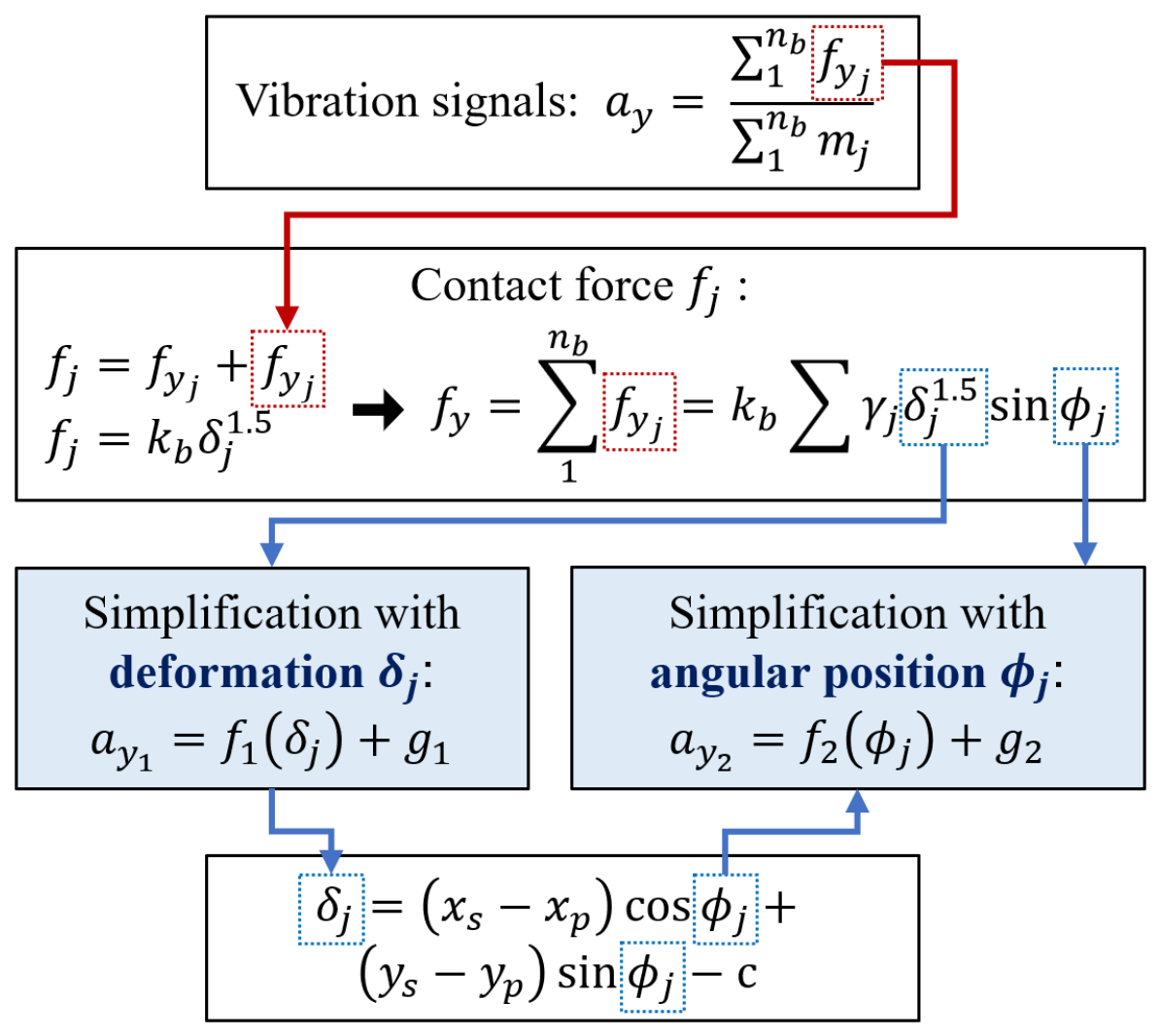
As given in Equations (14)–(16), the vertical acceleration a y can be considered as the output of a complex nonlinear model during the bearing life cycle. The process for extracting the fundamental physical variables and simplifying the equations related to acceleration is sketched in Figure 5. The model can be simplified to a function with the exponential function of δ j as the independent variable and a y 1 as the output acceleration signal. Further, another form of the simplified model is a function with the trigonometric function ϕ j as the independent variable and a y 2 as the output acceleration signal. The first simplification of a y can be made as Equation (19):
a y 1 = m 1 k b j = 1 n b γ j δ j 1.5 sin ϕ j = f y ( δ j 1.5 ) + g 1 = f y 1 ( δ j ) + g 1 ,
where f y 1 is an exponential function of the independent variable δ j with all other system perturbations termed as g 1 . The exponential function can be the basis function in the simplification of a y 1 . It corresponds to the polynomial library in the SINDy-NN. By using this library, the function a y 1 with δ j 1.5 as the variable can be represented by a coefficient matrix and a sparse matrix of basis functions ( z 0 , z 1 , z 2 , z 3 , …, z n D , with the degree n D N + ). The degree n D represents the highest order of polynomial functions in the feature library.
The second simplification denoted by f y 2 is a trigonometric function of the independent variable ϕ j with all other system perturbations termed as g 2 , as presented by Equation (20):
a y 2 = m 1 k b j = 1 n b γ j δ j 1.5 sin ϕ j = f y ( sin ( ϕ j ) , cos ( ϕ j ) ) + g 2 = f y 2 ( ϕ j ) + g 2 ,
where substituting Equation (18) into the term δ j 1.5 sin ϕ j gives Equation (21):
δ j 1.5 sin ϕ j = ( y s y p ) 1.5 ( sin ϕ j ) 2.5 + 1.5 ( x s x p ) ( y s y p ) 1.5 ( sin ϕ j ) 1.5 cos ϕ j 1.5 c ( y s y p ) 1.5 ( sin ϕ j ) 1.5 + 0.75 ( y s y p ) 0.5 ( x s x p ) 2 ( sin ϕ j ) 0.5 ( cos ϕ j ) 2 1.5 c ( x s x p ) ( y s y p ) 0.5 ( sin ϕ j ) 0.5 cos ϕ j + 0.75 c 2 ( y s y p ) 0.5 ( sin ϕ j ) 0.5 .
The simplified mechanism model can avoid the complicated calculation in Equation (21) and provides a basis for the definition of the feature library. The trigonometric function in the simplification of a y 2 can correspond to basis functions in the Fourier library. By using the Fourier library, the function a y 2 with ( cos ( ϕ j ) ) 0.5 , ( sin ( ϕ j ) ) 1.5 , ( cos ( ϕ j ) ) 2 , and ( sin ( ϕ j ) ) 2.5 as the variables can be represented by a coefficient matrix and a sparse matrix of basis functions ( sin z , cos z , sin 2 z , cos 2 z , sin 3 z , cos 3 z ,…, sin ( n F z ) , cos ( n F z ) ), with the frequency number n F N + . The frequency number n F increments in integers and represents the highest function order in the Fourier library.

3. Test Bench and Data Processing

3.1. Introduction of Test Bench and Dataset

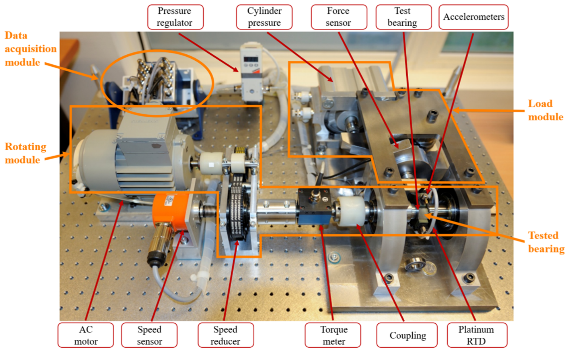
The dataset used in this study is obtained from the PRONOSTIA platform. As shown in Figure 6, the test bench includes components for rotation, a loading module for accelerated run-to-failure testing, and a measurement part. Here, “accelerated run-to-failure testing” denotes the progressive deterioration of the bearing health state under high rotational speed and radial load, as reflected by changes in the vibration response. It does not imply that a specific final failure mode is assumed in advance. The tested bearings are NSK 6804DD deep-groove ball bearings. This bearing type is a single-row rolling ball bearing with double rubber contact seals and a grease-lubricated configuration according to the bearing specification. The public dataset does not specify the grease grade; therefore, only the lubrication state is reported here. The asynchronous motor has a power rating of 250 W and a nominal speed of 2830 rpm [37]. The pneumatic loading module applies a radial load through a lever mechanism. Accordingly, the 4000 N, 4200 N, and 5000 N load values in Table 1 are radial loads. The vibration sensor consists of two miniature accelerometers positioned at 90° relative to each other. Acceleration measurements are sampled at 25.6 kHz in 0.1-s recordings, with a 10-s interval between recordings. The dataset includes 17 bearings subjected to accelerated run-to-failure tests, as summarized in Table 1. Because the public dataset does not provide post-test inspection results, the final failure mode is not further specified in this study. In these experiments, a bearing is considered to have failed when the acceleration amplitude exceeds 20 g. Three distinct operating conditions are used in the accelerated run-to-failure tests.

3.2. Aging Phase Division

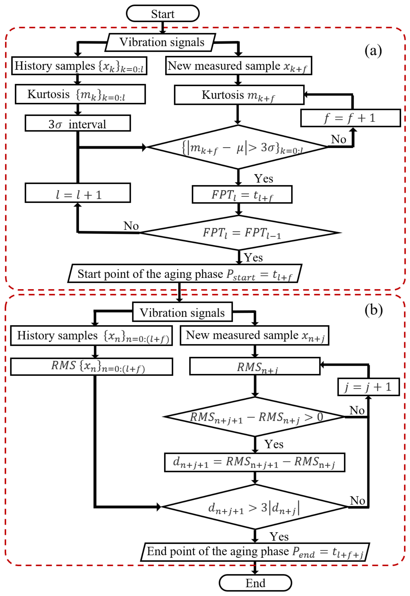
Since the ultimate target of this research is to apply SINDy-NN for modeling bearing fault dynamics, a prerequisite is to identify the measurement data corresponding to the onset of bearing failure. Typically, the entire life cycle of a bearing can be divided into three phases: run-in, linear aging, and exponential aging. This section focuses on the segmentation of the aging phase and the associated data processing. The complete process for determining the aging phase is illustrated in Figure 7.
Since kurtosis is sensitive to early-stage failures [38], it is employed to determine the starting point of the aging phase. The Root Mean Square (RMS) of acceleration is used to distinguish between the aging and failure stages. An adaptive method based on the 3 σ interval ( [ μ 3 σ , μ + 3 σ ] ) is used to determine the starting point of the aging phase, namely the selection of the First Predicting Time (FPT) in [38]. The 3 σ interval is adopted here as a commonly used control-limit criterion in statistical process control and engineering abnormality detection [39,40]. This is determined by calculating the mean value μ and standard deviation σ of kurtosis using historical data from the healthy phase. When a new peak state m f is available at a time point t f and exceeds the 3 σ interval, the health state of bearing is considered abnormal. To reduce false alarms caused by isolated fluctuations, the final FPT is determined only when consecutive kurtosis values continuously exceed the threshold. As shown in Figure 7a, when consecutive l + 1 kurtosis values m f + k k = 0 : l satisfy m f + k μ > 3 σ k = 0 : l , time t l + f is chosen as FPT l . l starts from zero and increases until FPT l = FPT l 1 is satisfied, and then FPT l is output as the final FPT value, which means the starting point of the aging phase. Likewise, RMS and the 3 σ interval are combined for identifying the aging and failure phases. As outlined in Figure 7b, when the RMS of the newly measured sample is greater than that of the last tested sample, their difference is extracted as d j . If d n + j + 1 > 3 d n + j , then t l + f + j is determined as the starting point of the bearing failure phase.
Prior to segmentation, Stationary Wavelet Transform (SWT) is applied to filter the raw signal, as SWT mitigates the translation-invariance issue associated with Discrete Wavelet Transform (DWT) by upsampling the filter coefficients at each level [41,42]. Moreover, SWT has been proven effective for decomposing acceleration signals in bearing fault diagnosis [43,44]. The filter frequency resolution is set to 50 Hz, and the number of layers is determined by the criterion that the frequency resolution of the final layer must be less than 50 Hz. Each test sample consists of 2560 vibration data points collected within a continuous sampling period of 0.1 s. No sliding window is employed, as the interval between consecutive samples is 10 s.
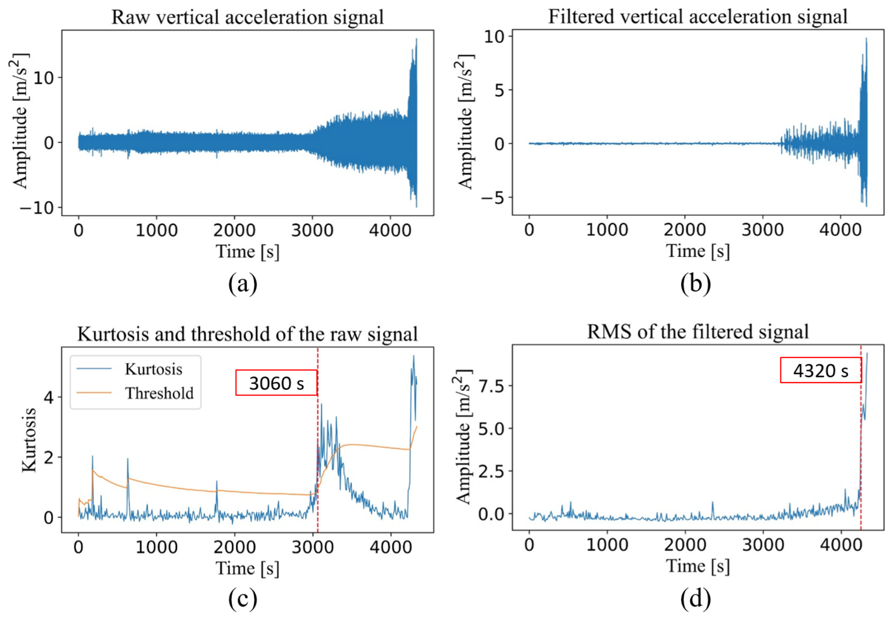
Figure 8a,b display the raw and filtered acceleration measurements of Bearing 3_3, respectively. It is evident that noise-induced fluctuations are reduced after filtering, while the fluctuations caused by the bearing’s aging and failure become more pronounced. This filtering result is considered valid, as it simplifies the assessment of bearing health by minimizing abnormal signal fluctuations. Figure 8c,d present the identification results for the aging and failure points. After filtering, a more distinct trend and greater magnitude of change in kurtosis and RMS are observed. These two features, combined with the 3 σ interval, effectively identify the aging stages. For example, in Bearing 3_3, the boundary between the run-in and linear aging phases is identified at 3060 s, while the exponential aging phase begins at 4320 s. This exact procedure is applied to all bearings to extract the measurement data at the failure stage for subsequent modeling.

4. Modeling with Standard Libraries

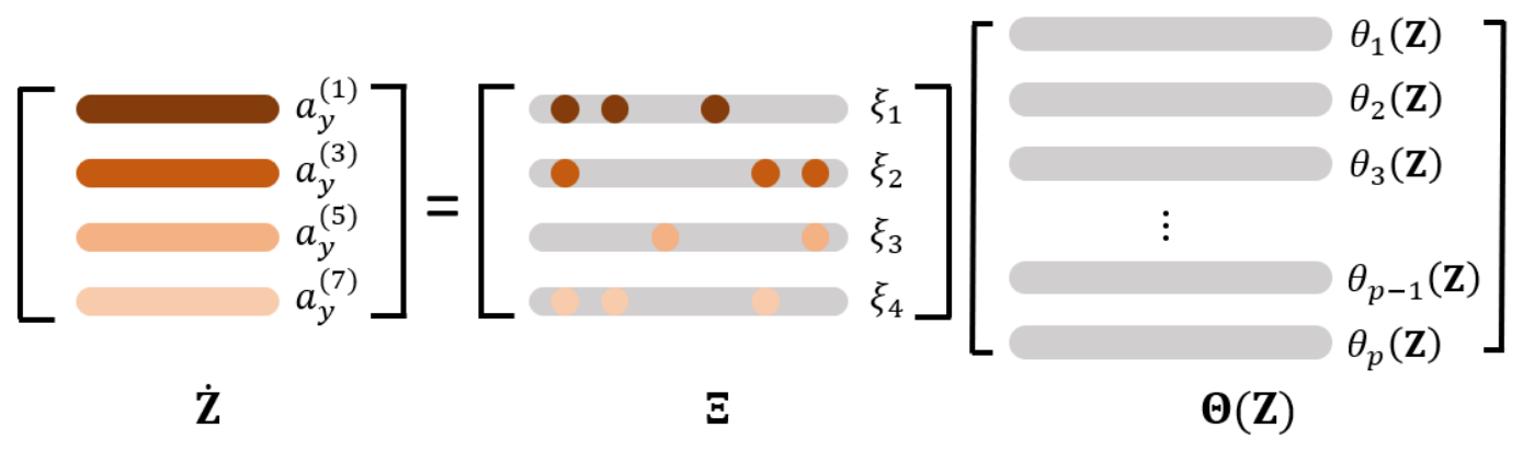
Given the close relationship between polynomial and Fourier functions and the underlying mechanism model, efforts are made to construct an optimized feature library for SINDy-NN to enhance modeling efficiency, accuracy, and interpretability. This section examines the influence of polynomial and Fourier basis functions on SINDy modeling accuracy to identify the optimal combination of basis functions. Subsequently, the two types of basis functions are combined to improve modeling accuracy, and the approach is validated on other bearings. The proposed method is validated using data from the PRONOSTIA platform, with the coefficient of determination ( R 2 ) selected as the evaluation metric for modeling accuracy. Due to the 10-s sample recording interval, a modeling configuration is sought that balances accuracy ( R 2 0.90 ) with time consumption ( t train 10 s), as 0.90 is considered sufficiently high for R 2 in most engineering applications. Before investigating the impact of model dimensionality on modeling performance, a four-input–four-output model (model dimension n MD = 4 ) is constructed using a feature library of p candidate functions, with Bearing 3_3 serving as an example. The state construction of the MIMO model is detailed in the Appendix A. The inputs and outputs required for model identification are various orders of acceleration derivatives, where all outputs a y ( 2 n + 1 ) ( n = 0 , 1 , 2 , 3 ) in Z ˙ are one order higher than the inputs a y ( 2 n ) ( n = 0 , 1 , 2 , 3 ) in Z , as shown in Figure 9. Table 2 lists some critical parameters of the network and training.

4.1. Fourier Library

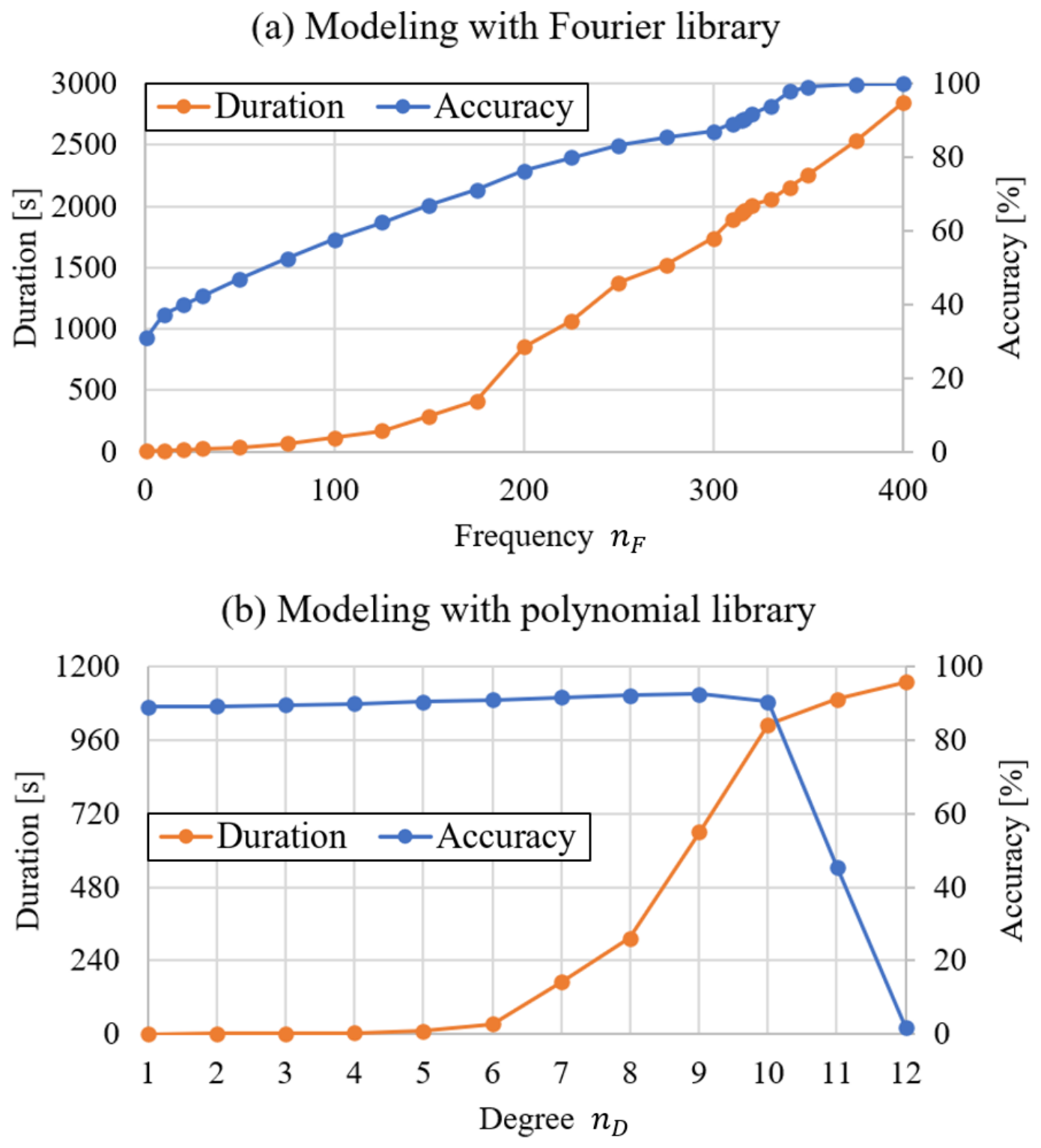
As the form of basis functions extracted in the simplification of a y 2 , Fourier series are also widely used in signal modeling. We first study the impact of the Fourier library configuration on the modeling accuracy of SINDy-NN. n F represents the highest frequency of the trigonometric functions in the Fourier library. When n F = 2 , the basis functions are sin x i , cos x i , sin 2 x i , and cos 2 x i   ( i = 1 , 2 , 3 , 4 ) . Figure 10a shows the accuracy of the fitted model using the Fourier library with different configurations. The bearing model uses 2560 sampling points and the finite differences in different orders they generate. This means that the feature library with n F = 400 and n MD = 4 provides 3200 basis functions (number of Fourier basis function n Fcn F = 2 n F n MD , including sin ( n x i ) and cos ( n x i ) , where n = 1 , 2 , 3 , , 400 and i = 1 , 2 , 3 , 4 ). However, it takes 2841 s to build the model with 99.99% accuracy, which reflects the inefficiency of modeling and makes practical application difficult. Besides, the modeling accuracy is low when n F is small, which means few basis functions.
However, in the present bearing acceleration modeling task, a Fourier-only library shows limited modeling efficiency. When n F is small, the number of trigonometric basis functions is insufficient to represent the dominant acceleration-generating components. When n F is increased to improve accuracy, the number of Fourier terms and the training time increase substantially. Therefore, this result does not indicate that Fourier functions are generally ineffective. Instead, it suggests that Fourier basis functions alone are not compact enough for this task. One possible reason is that the measured bearing acceleration contains not only periodic components related to rolling element motion but also nonlinear contact-force components associated with deformation. Thus, a combined feature library is needed to represent both periodic angular-position terms and contact-related nonlinear terms more efficiently. Nevertheless, the Fourier library still provides useful periodic basis functions. As n F increases, the modeling accuracy improves continuously, although this improvement is accompanied by a substantial increase in the number of basis functions and training time. This observation supports the use of Fourier terms as auxiliary components in the custom library rather than as the only basis-function type.

4.2. Polynomial Library

The polynomial library, as the form of basis functions extracted in the simplification of a y 1 , is a key focus of this research due to its strong fitting capability. The degree n D represents the highest order of polynomial functions within the library. For example, when n D = 2 and n MD = 4 , the basis functions consist of 1, x i 1 , and x i 1 x i 2 ( i 1 , i 2 = 1 , 2 , 3 , 4 and i 2 i 1 ) . It is worth noting that the number of polynomial basis functions n Fcn P does not exhibit proportional growth like the Fourier function but instead demonstrates a similar exponential increase with the rise in n D , as shown in Equation (22):
n Fcn P = n MD + n D n D = i = 0 n MD 1 ( n MD + n D i ) n MD ! .
Figure 10b shows the accuracy of the fitted models using a polynomial library with various configurations. When n D = 1 , modeling achieves an accuracy of 89.08% with a duration of 0.92 s. For n D = 5 , accuracy increases to 90.37%, but it requires 10.40 s. Thus, a sub-conclusion can be drawn: the modeling efficiency of the polynomial library is high when n D is relatively low. As n D increases within the range [ 1 , 9 ] , modeling accuracy rises gradually, peaking at 92.43%. Beyond this point, accuracy declines rapidly as n D increases further. Therefore, it is reasonable to assume that there is an upper limit to the modeling accuracy when using the polynomial library. Increasing the number of basis functions negatively affects the modeling accuracy when the upper limit is reached. Presumably, this is caused by overfitting. According to Equation (22), at n D = 10 , there are 1001 basis functions, with a majority being high-order terms. When n D increases to 11, high-order polynomials account for 97.4% of the basis functions. The significant presence of these high-order terms leads to overfitting during network training, causing a decrease in accuracy after the peak is reached.
Notably, the modeling time rises substantially once n D = 6 , while the corresponding accuracy improvement remains marginal, indicating a decline in modeling efficiency. This inefficiency can be attributed to the sharp increase in the number of basis functions. Therefore, the polynomial library presents two primary limitations: high-order polynomials tend to cause overfitting, and modeling efficiency diminishes significantly once n D surpasses a certain threshold. These adverse effects need to be addressed in future research on feature libraries.

4.3. Model Dimensionality

In addition to library configuration, model dimensionality (latent dimension of Z ˙ in Figure 3 and Figure 9 is a critical modeling parameter. The model dimensionality n MD in virtual state theory equals the dimensionality of model inputs, as detailed in the Appendix A. The Fourier library achieves 90% accuracy in 1962.9 s, while the polynomial library only requires 10.4 s. It means that the polynomial library is nearly 189 times faster than the Fourier library with t train 10 s. Therefore, we employ polynomials for experiments on model dimensions. Figure 11 shows the accuracy of the fitted model using a polynomial library with different model dimensions n MD . We used the measured signals and their finite differences as inputs ( a y ( i ) , i = 0 , 1 , 2 , , n MD 1 , where n MD N ).
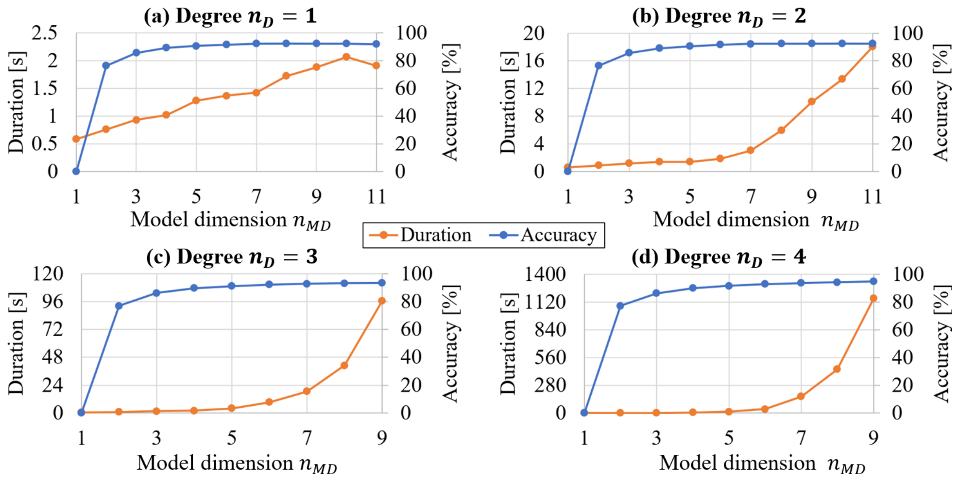
Figure 11 illustrates that, as the model dimension n MD increases, the modeling accuracy growth rate decelerates while the time consumption growth rate accelerates. Such trends are observed using different n D . By focusing on the modeling accuracy among the four graphs, it can be seen that the upper limit of modeling accuracy will increase as degree n D increases. The performance of the MIMO model is much better than that of the Single-Input-Single-Output (SISO) model ( n MD = 1 ). This is because, when using the same library, the amount of input data used for training the neural network and the number of function components in the SISO model are much fewer than in the MIMO model. When considering modeling time for efficiency requirements, models with n MD 8 offer no advantage due to their excessive time consumption. Given that the modeling accuracy does not exceed 90.00% within ten seconds when n D 4 , experiments based on higher n D will no longer be shown and discussed. As can be seen from the time curve in Figure 11, it is very time-consuming to build a high-precision model by adding n MD and n D . It can be concluded that models with a low dimension n MD or a low degree n D can better meet the requirements of modeling efficiency.

5. Modeling with Custom Library

5.1. Construction of Custom Library

Modeling experiments with standard libraries reveal that polynomial libraries frequently lead to overfitting, with limited scope for improving accuracy. Furthermore, Fourier basis functions exhibit relatively low modeling efficiency. The aim is to address these challenges by constructing a customized library that balances accuracy and efficiency.
The design of the customized library is grounded in rigorous mechanism analysis and sufficient experimental data. Equations (16) and (18) provide mechanistic justification for selecting polynomial and Fourier functions as basis functions based on characteristics observed during experiments, forming a solid foundation for constructing the customized library.
Informed assumptions can be made based on the experimental findings. Low-order polynomials can serve as the core components in the customized library, providing the necessary performance for rapid and accurate modeling. The quantities of low-order polynomials, determined by n D and n MD , should be prioritized and configured. As auxiliary components, Fourier functions can stabilize and enhance modeling accuracy. The number of Fourier basis functions is determined by n MD and n F . Therefore, the process of constructing the polynomial library can be divided into three steps. The first step is determining the range of n D within the training time limit to ensure that accuracy and computational time meet the basic requirements. The second step is configuring the model dimension n MD to maximize the utility of the core components within the time limit. The third step is configuring the frequency n F to maximize the functionality of the auxiliary components within the training time limit.

5.2. Modeling Results

Corresponding experiments can be performed using the proposed custom library construction process. First of all, according to Figure 11, when n D 3 , the polynomial library can meet the requirements of accuracy R 2 0.90 and time consumption t train 10 s. Then, three groups of experiments with different n D 3 were carried out, as shown in Table 3. Second, for each degree n D , we select the several model dimensions n MD with the highest modeling accuracy within ten seconds to improve the modeling accuracy as much as possible. For example, when n D = 1 , the polynomial basis function reaches its maximum value at n MD = 8 in only 1.72 s. Finally, within the specified time limit t train 10 s, Fourier basis functions ( n F = 1 , 2 , , 8 ) of various frequencies are added to improve modeling accuracy.
To facilitate a more comprehensive comparison of modeling efficiency, the polynomial and Fourier libraries, configured with the most efficient settings, are utilized to construct baseline models at the bottom of Table 3, respectively. A standard feature library, such as Base_Poly2, requires 66 times the duration to attain an accuracy exceeding 90.00% compared to libraries No.5, No.9, No.11, and No.17. Another baseline model utilizing a Fourier library takes 2002.42 s to achieve a comparable level of accuracy. It can be speculated that the basis function number n Fcn ( n Fcn = n Fcn F + n Fcn P ) is the primary factor affecting the modeling duration. The mechanism-based optimization of the basis function configuration reduces computational complexity by decreasing the number of basis functions, thus improving model fitting speed.
Table 4 provides an additional benchmark comparison beyond the feature-library comparisons within the SINDy-NN framework. The LSTM model achieves the highest validation accuracy, showing its strong sequence-fitting capability for this specific acceleration signal. However, the LSTM model remains a black-box predictor and does not yield an explicit sparse dynamic equation. The proposed SINDy-NN achieves slightly lower accuracy but requires less modeling time and preserves a physically traceable sparse representation. Meanwhile, the lower accuracies of TCN and PatchTransformer indicate that more complex sequence architectures do not automatically lead to better performance for this limited-state bearing dynamics identification task. These results suggest that the proposed method offers a balanced solution in terms of accuracy, efficiency, sparsity, and physical interpretability.
Overall, these results show that the proposed custom library does not simply pursue the highest black-box fitting accuracy. Instead, it provides a compact and physically traceable sparse model with competitive accuracy and relatively low modeling cost. This balance among accuracy, modeling time, sparse representation, and interpretability is the main advantage of the mechanism-guided SINDy-NN in this study.

5.3. Validation Across Different Bearings

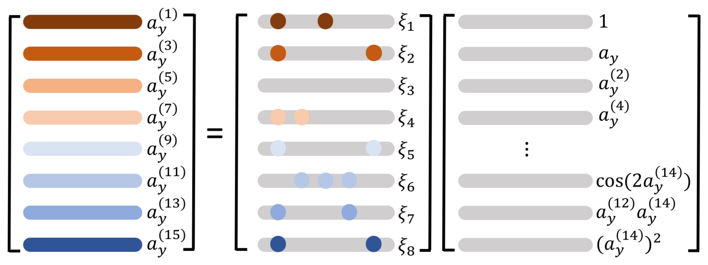
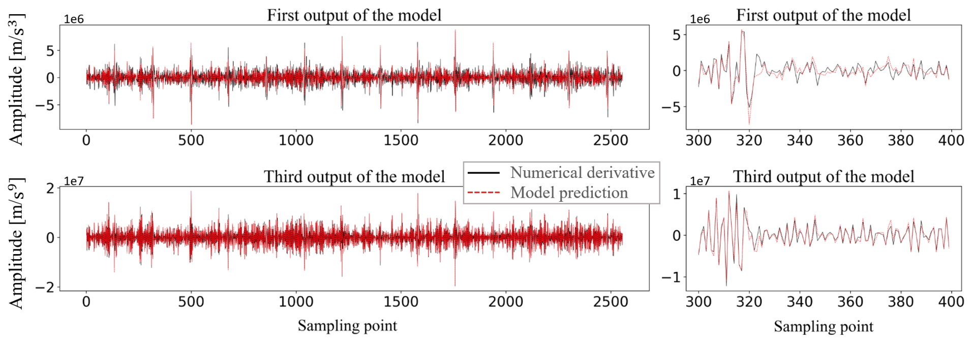
Among all custom libraries, Library No. 11 achieves the highest modeling accuracy with n D = 2 , n MD = 8 , and n F = 2 , representing the optimal configuration for bearing fault modeling in this study. Figure 12 illustrates the eight-input, eight-output model structure. Figure 13 compares the raw data with model outputs for the first and the fourth dimensions. The subfigures on the right provide a zoomed-in view of the curves corresponding to 100 sampling points from the subfigures on the left. As the output order increases, the model’s accuracy improves, capturing signal fluctuations more effectively. However, the model’s performance in fitting spikes is relatively limited, as noise amplification occurs when finite differences are used to generate data. This limitation arises from the data generation method rather than the underlying mechanism. In future work, the design of a differential observer could replace direct finite differences, mitigating this issue. The high similarity between the red and black curves indicates that SINDy-NN, when equipped with a custom library based on a simplified mechanism, can achieve high accuracy efficiently while avoiding overfitting.
The modeling results for Bearing 3_3 provide insight into the optimal feature library and model dimension for SINDy-NN in bearing dynamics modeling. Additional models are built using SINDy-NN to investigate whether the configured custom library can be applied to bearings under other operating conditions. Table 5 presents the sample numbers and modeling results for each bearing. The selected modeling configuration achieves slightly lower accuracy in bearings under Condition 2 and higher accuracy in those under Condition 1. It is hypothesized that the lower load force in Condition 1 reduces operational noise, resulting in higher signal quality and, consequently, higher modeling accuracy. Despite these variations, sufficiently high accuracy and low standard deviation are obtained for all bearings, further verifying the applicability of SINDy-NN to bearing dynamics modeling.

6. Conclusions

This research introduces a physics-informed SINDy-NN model, which constructs its feature library by extracting basis functions from a simplified mechanism model to enhance the efficiency and interpretability of SINDy-NN-based modeling. The proposed approach has been validated using experimental data from a bearing test bench. The main conclusions of this research are summarized as follows:
1.
A feature library integrated with a simplified mechanism significantly improves the modeling efficiency of the SINDy network.
2.
The custom library reduces the number of candidate terms required for bearing acceleration modeling while retaining the main contact-related components suggested by the 5-DoF mechanism. This makes the identified SINDy equations easier to inspect than models built from large standard libraries.
3.
The combination of SINDy-NN with mechanism enables efficient modeling of bearing dynamics.
4.
The 3 σ interval method utilizing kurtosis and RMS provides a practical classification of bearing aging phases.
While the proposed method demonstrates promise, several limitations remain. First, the custom feature library is derived from simplified Hertzian contact assumptions, so the contact-related basis functions may need to be re-examined for lubricated, rough, coated, composite, or otherwise non-Hertzian contact systems. Second, finite-difference-based Multi-Input–Multi-Output (MIMO) state construction may amplify noise, especially under high-order differentiation or abrupt changes in rotational speed and load. Third, the present framework identifies system-level bearing dynamics from vibration responses and does not explicitly model local Elastohydrodynamic Lubrication (EHL) film-thickness effects. These limitations motivate the following future work:
1.
Future work may extend the mechanism-guided basis functions toward lightweight and interpretable neural network design. The contact-related terms identified in this study could serve as structural priors or kernels for downstream tasks such as fault classification and RUL prediction.
2.
When tribological measurements are available, lubricant properties, temperature, surface roughness, and film-thickness information could be introduced as additional physics-guided candidate terms, such as the minimum film thickness h min , film parameter λ , or viscosity ratio κ .
3.
Robust derivative estimators or observer-based state construction methods should be developed to reduce noise amplification in finite-difference-based MIMO states, especially under abrupt changes in rotational speed, load, or other operating conditions.

Author Contributions

Conceptualization, Y.F.; methodology, L.Z.; software, L.Z.; validation, Z.L.; formal analysis, Y.F.; investigation, Z.W.; resources, Y.P.; data curation, Z.L.; writing—original draft preparation, L.Z.; writing—review and editing, Z.W.; visualization, Z.W.; supervision, K.Z.; project administration, K.Z.; funding acquisition, Y.F. All authors have read and agreed to the published version of the manuscript.

Funding

This research was funded by Dongfang Turbine Co., Ltd. under the project “Cloud-Based Intelligent and Lightweight Operation and Maintenance of Turbine Power Equipment” (Grant No. DEC8300CG202419749A1228111), and was supported by the Zhejiang Provincial Postdoctoral Scientific Research Merit-Based Funding Project (Grant No. ZJ2025216).

Data Availability Statement

The original data presented in the study are openly available at https://github.com/wkzs111/phm-ieee-2012-data-challenge-dataset (accessed on 26 May 2026).

Conflicts of Interest

Author Yan Ping was employed by the company Dongfang Turbine Co., Ltd. The remaining authors declare that the research was conducted in the absence of any commercial or financial relationships that could be construed as a potential conflict of interest.

Abbreviations

The following abbreviations are used in this manuscript:
SINDy-NNSparse Identification of Nonlinear Dynamics-based Neural Network
5-DoFFive Degrees of Freedom
MIMOMulti-Input–Multi-Output

Appendix A. Virtual State

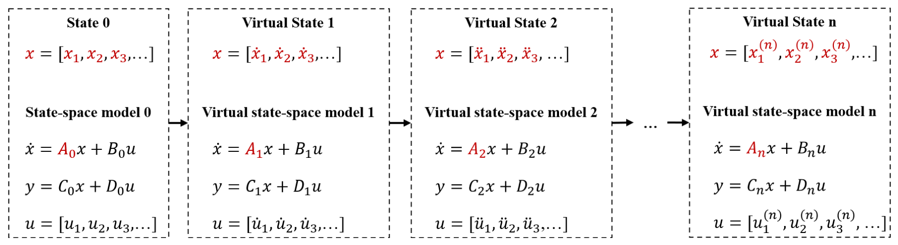
We proposed the concept of the virtual state in a system with some physical meaning that does not need to be precisely defined. Since virtual states x i are inferred from the initially simulated physical models, the first-order and higher-order derivatives ( x ˙ i , x ¨ i , , x i ( n ) ) of the virtual state x i are still virtual states representing the rate of change in the virtual state x i ( n 1 ) . Moreover, it is reasonable to assume that the model’s input or output vector can be obtained from the first-order to multiple-order derivations of some measurable state or output variables, corresponding to the generation of the high-order virtual states. Figure A1 illustrates the continuous modeling with a series of virtual states x ˙ i , x ¨ i , , x i ( n ) ( i , n N + ) from one order to multiple orders, along with a series of model inputs u ˙ i , u ¨ i , , H u i ( n ) ( i , n N + ) .
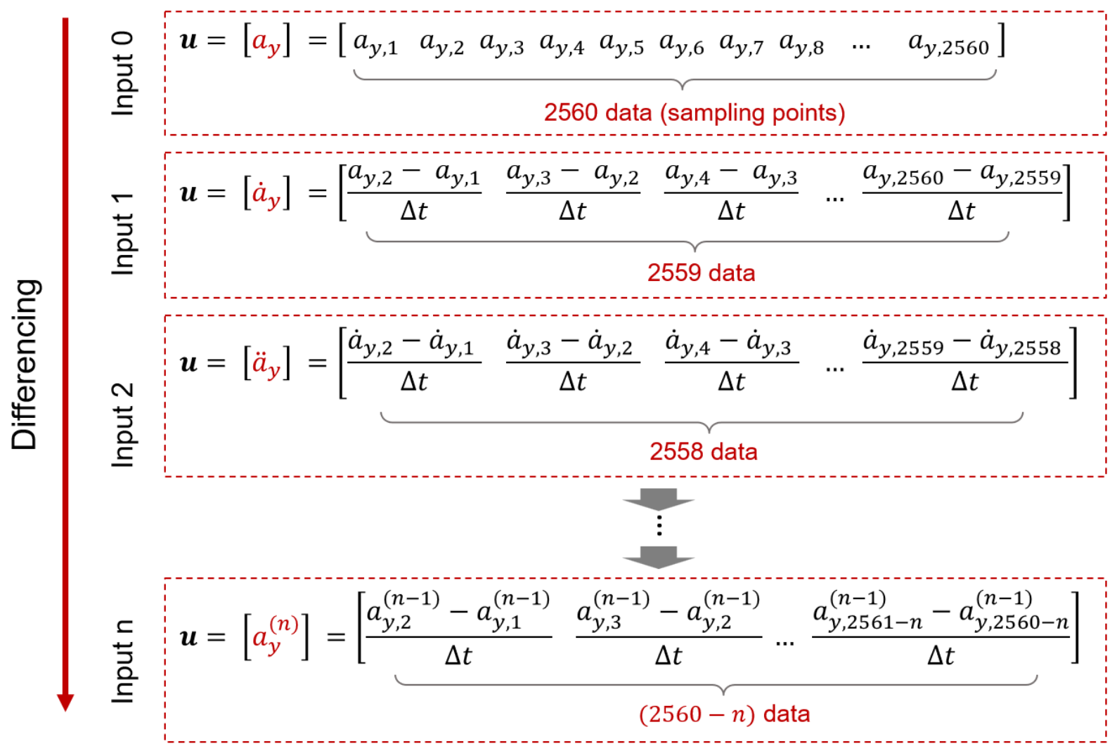
According to the description of the generating data of more dimensions, the acceleration signal can be differentiated in multiple orders to obtain data for input and output. Since the sampling frequency is 25.6 kHz, the time interval between each sample point is short enough to process the input data using finite difference rather than differentiation. By taking a recording sample of the FEMTO bearing dataset, multiple differencing processes of the raw signal can produce sufficient data for the need from data-driven methods, as shown in Figure A2.
Figure A1. Virtual states and virtual state-space models.
Machines 14 00620 g0a1
Figure A2. Generation of high-order input and output data by finite difference.
Machines 14 00620 g0a2

References

  1. He, L.; Yang, F.; Li, Z.; Yan, J.; Ruan, D. Modeling of the race roundness and roughness for ball bearing based on fourier series and fractal theory. Results Eng. 2025, 25, 104469. [Google Scholar] [CrossRef] [Scilit]
  2. Li, Z.; Kornhardt, G.; Ruan, D. Bearing Fault Classification Based on Pole-Zero Distribution of Transfer Function. In Proceedings of the 2023 CAA Symposium on Fault Detection, Supervision and Safety for Technical Processes (SAFEPROCESS); IEEE: New York, NY, USA, 2023; pp. 1–6. [Google Scholar]
  3. Xi, S.; Cao, H.; Chen, X.; Niu, L. Dynamic modeling of machine tool spindle bearing system and model based diagnosis of bearing fault caused by collision. Procedia CIRP 2018, 77, 614–617. [Google Scholar] [CrossRef] [Scilit]
  4. Li, K.; Tang, W. Load-displacement relationship model and measurement of deep groove ball bearing and 4-point contact ball bearing. J. Mech. Sci. Technol. 2021, 35, 3045–3058. [Google Scholar] [CrossRef] [Scilit]
  5. Gao, S.; Chatterton, S.; Pennacchi, P.; Han, Q.; Chu, F. Skidding and cage whirling of angular contact ball bearings: Kinematic-hertzian contact-thermal-elasto-hydrodynamic model with thermal expansion and experimental validation. Mech. Syst. Signal Process. 2022, 166, 108427. [Google Scholar] [CrossRef] [Scilit]
  6. Cui, L.; Chen, X.; Chen, S. Dynamics modeling and analysis of local fault of rolling element bearing. Adv. Mech. Eng. 2015, 7, 262351. [Google Scholar] [CrossRef] [Scilit]
  7. Mishra, C.; Samantaray, A.; Chakraborty, G. Ball bearing defect models: A study of simulated and experimental fault signatures. J. Sound. Vib. 2017, 400, 86–112. [Google Scholar] [CrossRef] [Scilit]
  8. Singh, J.; Darpe, A.; Singh, S.P. Bearing remaining useful life estimation using an adaptive data-driven model based on health state change point identification and K-means clustering. Meas. Sci. Technol. 2020, 31, 085601. [Google Scholar] [CrossRef] [Scilit]
  9. Ruan, D.; Gühmann, C.; Yan, J. A new solving method for ball bearing dynamics model based on optimization with nonlinear constraints: Contact angles as iterative variables. J. Manuf. Process. 2023, 106, 338–346. [Google Scholar] [CrossRef] [Scilit]
  10. Jiang, G.; Zhou, K.; Li, Z.; Yan, J. Bearing Dynamics Modeling Based on the Virtual State-Space and Hammerstein–Wiener Model. Sensors 2024, 24, 5410. [Google Scholar] [CrossRef] [Scilit] [PubMed]
  11. Kaheman, K.; Kutz, J.N.; Brunton, S.L. SINDy-PI: A robust algorithm for parallel implicit sparse identification of nonlinear dynamics. Proc. R. Soc. A 2020, 476, 20200279. [Google Scholar] [CrossRef] [Scilit]
  12. Omar, M.; Li, R.; Asker, A. A framework for data driven dynamic modeling of serial manipulators. IEEE Access 2022, 10, 124874–124883. [Google Scholar] [CrossRef] [Scilit]
  13. Arora, R.; da Silva, B.C.; Moss, E. Model-Based Reinforcement Learning with SINDy. arXiv 2022, arXiv:2208.14501. [Google Scholar] [CrossRef] [Scilit]
  14. Lenfesty, B.; Bhattacharyya, S.; Wong-Lin, K. Uncovering dynamical equations of stochastic decision models using data-driven SINDy algorithm. arXiv 2024, arXiv:2406.01370. [Google Scholar] [CrossRef] [Scilit]
  15. Er, M.B.; Koca, T. A Novel Approach for Motor Bearing Fault Detection Using EMD-Based Denoising and Detrended Fluctuation Analysis & LSTM Multimodal Hybrid Features with K-Means Clustering. J. Vib. Eng. Technol. 2026, 14, 103. [Google Scholar]
  16. Koca, T.; Er, M.B.; Çıtlak, A. Transformer-Based Bearing Fault Classification with VMD-Based Noise Suppression and rCCA-Enhanced Correlation Modeling. Machines 2026, 14, 507. [Google Scholar] [CrossRef] [Scilit]
  17. Liu, Q.; Zhang, Y.; Si, X.; Fan, Z. DLVR-NWP: A Novel Data-Driven Bearing Degradation Model for RUL Estimation. IEEE Trans. Instrum. Meas. 2023, 72, 3508309. [Google Scholar] [CrossRef] [Scilit]
  18. Zhao, Y.; Zhu, Y.P.; Lin, J.; Han, Q.; Liu, Y. Analysis of nonlinear vibrations and health assessment of a bearing-rotor with rub-impact based on a data-driven approach. J. Sound Vib. 2022, 534, 117068. [Google Scholar] [CrossRef] [Scilit]
  19. Babin, A. Data-driven system identification and optimal control of an active rotor-bearing system. In Proceedings of the IOP Conference Series: Materials Science and Engineering; IOP Publishing: Bristol, UK, 2021; Volume 1047, p. 012053. [Google Scholar]
  20. Hamadache, M.; Jung, J.H.; Park, J.; Youn, B.D. A comprehensive review of artificial intelligence-based approaches for rolling element bearing PHM: Shallow and deep learning. JMST Adv. 2019, 1, 125–151. [Google Scholar] [CrossRef] [Scilit]
  21. Li, Z.; Ruan, D.; Chen, X.; Qian, Y.; Yan, J.; Gühmann, C. Mutually Complementary: Physics-informed GAN based on Simulated Model for Fault Diagnosis. In Proceedings of the 2025 IEEE International Conference on Prognostics and Health Management (ICPHM); IEEE: New York, NY, USA, 2025; pp. 1–8. [Google Scholar]
  22. Ge, J.; Yao, Z.; Wu, M.; Almeida, J.H.S., Jr.; Jin, Y.; Sun, D. Tackling data scarcity in machine learning-based CFRP drilling performance prediction through a broad learning system with virtual sample generation (BLS-VSG). Compos. Part B Eng. 2025, 305, 112701. [Google Scholar] [CrossRef] [Scilit]
  23. Ruan, D.; Li, Z.; Wu, Y.; Yan, J.; Gühmann, C. Fuzzy-membership-based labeling: A new labeling method for both classification task and regression task. In Proceedings of the PHM Society Asia-Pacific Conference, Tokyo, Japan, 11–14 September 2023; Volume 4. [Google Scholar]
  24. Li, Z.; Wang, J.; Ruan, D.; Yan, J.; Gühmann, C. Bearing Digital Twin Based on Response Model and Reinforcement Learning. Lubricants 2023, 11, 502. [Google Scholar] [CrossRef] [Scilit]
  25. Ruan, D.; Wang, Y.; Qian, Y.; Yan, J.; Li, Z. Deep stacked state-observer based neural network (dsso-nn): A new network for system dynamics modeling and application in bearing. Adv. Eng. Inform. 2025, 65, 103357. [Google Scholar] [CrossRef] [Scilit]
  26. Wu, J.; Ruan, D.; Qian, Y. An Improved Physics-Guided Interpretable Inception Network and Its Application in Bearing Fault Diagnosis. IEEE Trans. Instrum. Meas. 2026, 75, 2502614. [Google Scholar] [CrossRef] [Scilit]
  27. Brunton, S.L.; Proctor, J.L.; Kutz, J.N. Discovering governing equations from data by sparse identification of nonlinear dynamical systems. Proc. Natl. Acad. Sci. USA 2016, 113, 3932–3937. [Google Scholar] [CrossRef] [Scilit]
  28. Goodfellow, I.; Bengio, Y.; Courville, A. Deep Learning; MIT Press: Cambridge, MA, USA, 2016. [Google Scholar]
  29. Lusch, B.; Kutz, J.N.; Brunton, S.L. Deep learning for universal linear embeddings of nonlinear dynamics. Nat. Commun. 2018, 9, 4950. [Google Scholar] [CrossRef] [Scilit]
  30. Champion, K.; Lusch, B.; Kutz, J.N.; Brunton, S.L. Data-driven discovery of coordinates and governing equations. Proc. Natl. Acad. Sci. USA 2019, 116, 22445–22451. [Google Scholar] [CrossRef] [Scilit]
  31. Zhang, L.; Schaeffer, H. On the convergence of the SINDy algorithm. Multiscale Model. Simul. 2019, 17, 948–972. [Google Scholar] [CrossRef] [Scilit]
  32. Zheng, P.; Askham, T.; Brunton, S.L.; Kutz, J.N.; Aravkin, A.Y. A unified framework for sparse relaxed regularized regression: SR3. IEEE Access 2018, 7, 1404–1423. [Google Scholar] [CrossRef] [Scilit]
  33. Kingma, D.P.; Ba, J. A method for stochastic optimization. In Proceedings of the International Conference on Learning Representations (ICLR), San Diego, CA, USA, 7–9 May 2015; Volume 5, p. 6. [Google Scholar]
  34. Lee, K.; Trask, N.; Stinis, P. Structure-preserving sparse identification of nonlinear dynamics for data-driven modeling. In Proceedings of the Mathematical and Scientific Machine Learning; PMLR: Beijing, China, 2022; pp. 65–80. [Google Scholar]
  35. Corbetta, M. Application of sparse identification of nonlinear dynamics for physics-informed learning. In Proceedings of the 2020 IEEE Aerospace Conference; IEEE: New York, NY, USA, 2020; pp. 1–8. [Google Scholar]
  36. Ruan, D.; Chen, Y.; Gühmann, C.; Yan, J.; Li, Z. Dynamics Modeling of Bearing with Defect in Modelica and Application in Direct Transfer Learning from Simulation to Test Bench for Bearing Fault Diagnosis. Electronics 2022, 11, 622. [Google Scholar] [CrossRef] [Scilit]
  37. Nectoux, P.; Gouriveau, R.; Medjaher, K.; Ramasso, E.; Chebel-Morello, B.; Zerhouni, N.; Varnier, C. PRONOSTIA: An experimental platform for bearings accelerated degradation tests. In Proceedings of the IEEE International Conference on Prognostics and Health Management, PHM’12, Denver, CO, USA, 18–21 June 2012; IEEE Catalog Number: CPF12PHM-CDR; IEEE: New York, NY, USA, 2012; pp. 1–8. [Google Scholar]
  38. Li, N.; Lei, Y.; Lin, J.; Ding, S.X. An improved exponential model for predicting remaining useful life of rolling element bearings. IEEE Trans. Ind. Electron. 2015, 62, 7762–7773. [Google Scholar] [CrossRef] [Scilit]
  39. Grant, E.L.; Leavenworth, R.S. Statistical Quality Control; McGraw-Hill: New York, NY, USA, 1980; Volume 7. [Google Scholar]
  40. Kamran, A.; Guozhu, L.; Rafique, A.F.; Zeeshan, Q. ±3-Sigma based design optimization of 3D Finocyl grain. Aerosp. Sci. Technol. 2013, 26, 29–37. [Google Scholar] [CrossRef] [Scilit]
  41. Fowler, J.E. The redundant discrete wavelet transform and additive noise. IEEE Signal Process. Lett. 2005, 12, 629–632. [Google Scholar] [CrossRef] [Scilit]
  42. Shensa, M.J. The discrete wavelet transform: Wedding the a trous and Mallat algorithms. IEEE Trans. Signal Process. 1992, 40, 2464–2482. [Google Scholar] [CrossRef] [Scilit]
  43. Wang, J.; Ye, C.; Jiang, M.; Zhang, F.; Sui, Q. SWT-KELM-Based rolling bearing fault diagnosis method under noise conditions with different SNRs. Meas. Sci. Technol. 2022, 34, 015007. [Google Scholar] [CrossRef] [Scilit]
  44. Nistane, V.; Harsha, S. Performance evaluation of bearing degradation based on stationary wavelet decomposition and extra trees regression. World J. Eng. 2018, 15, 646–658. [Google Scholar] [CrossRef] [Scilit]
Figure 1. Overview of research structure and flowchart.
Machines 14 00620 g001
Figure 2. Autoencoder architecture in the SINDy-NN [30].
Machines 14 00620 g002
Figure 3. Model structure with intrinsic coordinates [30].
Machines 14 00620 g003
Figure 4. 5-DoF model of bearing (optimized from [10]).
Machines 14 00620 g004
Figure 5. Procedure of feature library extraction for SINDy-NN.
Machines 14 00620 g005
Figure 6. The PRONOSTIA platform [37].
Machines 14 00620 g006
Figure 7. Flowchart of dividing bearing aging phase: (a) determination of the starting point of aging phase [38]; (b) determination of the starting point of failure phase.
Machines 14 00620 g007
Figure 8. Data of Bearing 3_3: (a) raw acceleration measurement; (b) filtered acceleration; (c) kurtosis and starting point of the aging phase; (d) RMS and the starting point of the failure phase.
Machines 14 00620 g008
Figure 9. Four-input–four-output model structure.
Machines 14 00620 g009
Figure 10. Accuracy and duration of SINDy-NN-based modeling: (a) Fourier library; (b) polynomial library.
Machines 14 00620 g010
Figure 11. Accuracy and duration of SINDy-NN-based modeling: (a) n D = 1 ; (b) n D = 2 ; (c) n D = 3 ; (d) n D = 4 .
Machines 14 00620 g011
Figure 12. Model structure with the selected custom library.
Machines 14 00620 g012
Figure 13. Fitting performance and comparison of bearing with SINDy-NN.
Machines 14 00620 g013
Table 1. FEMTO bearing dataset [37].
Operating ConditionCondition 1Condition 2Condition 3
Training setBearing 1_1Bearing 2_1Bearing 3_1
Bearing 1_2Bearing 2_2Bearing 3_2
Test setBearing 1_3Bearing 2_3Bearing 3_3
Bearing 1_4Bearing 2_4
Bearing 1_5Bearing 2_5
Bearing 1_6Bearing 2_6
Bearing 1_7Bearing 2_7
Rotational speed1800 rpm1650 rpm1500 rpm
Radial force4000 N4200 N5000 N
Table 2. Network architecture and training settings of the SINDy-NN model.
Structure ParameterValueTraining ParameterValue
Encoder architecture 8 256 8 OptimizerAdam
Decoder architecture 8 256 8 Learning rate 0.001
Hidden-layer activationSigmoidBatch size1024
Output-layer activationLinearMaximum epochs500
Input dimension n MD 8 λ 1 for L d x / d t 0.5
λ 2 for L d z / d t 0.01
λ 3 for L reg 0.01
Table 3. Experiments for configurations of basis functions of a custom library.
Library n D n MD n F n Fcn R 2 t train [s]
No.1181250.92322.37
No.22410.92374.09
No.33570.92436.25
No.44730.92478.29
No.55890.92539.81
No.6271500.92314.20
No.72640.92366.03
No.83780.92417.68
No.94920.92459.85
No.1081610.92518.47
No.112770.92569.68
No.12351660.91084.39
No.132760.91125.17
No.143860.91166.49
No.154960.91197.82
No.1651060.91238.71
No.1761160.91279.59
No.1861960.920914.08
Base_Poly15401260.903710.40
Base_Poly29407150.9243660.29
Base_Fourier0431625280.90322002.42
Table 4. Benchmark comparison.
Model R 2 Time [s]
Long Short-Term Memory (LSTM)0.974725.54
Temporal Convolutional Network (TCN)0.5549233.15
PatchTransformer0.7526216.20
Proposed SINDy-NN0.92569.68
Table 5. Modeling accuracy of bearings under different working conditions.
Working
Condition
  BearingSample
Number
Accuracy
R 2
Standard
Deviation
Condition 1Bearing 1_27960.94150.0343
Bearing 1_37640.92100.0424
Bearing 1_43430.93510.0247
Condition 2Bearing 2_315430.87680.0576
Bearing 2_43750.86080.0394
Bearing 2_72240.86660.0497
Condition 3Bearing 3_1460.89370.0350
Bearing 3_2700.86940.0366
Bearing 3_31260.92560.0337
Disclaimer/Publisher’s Note: The statements, opinions and data contained in all publications are solely those of the individual author(s) and contributor(s) and not of MDPI and/or the editor(s). MDPI and/or the editor(s) disclaim responsibility for any injury to people or property resulting from any ideas, methods, instructions or products referred to in the content.