Real-Time Feasibility of Digital Twins for Process Control: A Computational Analysis

Abstract

Digital twins enable closed-loop process control in smart manufacturing, yet no quantitative mapping exists between controller computational complexity and achievable real-time performance class. This paper aims to establish a quantitative mapping between controller computational complexity and achievable real-time performance class in digital twin-based process control, providing evidence-based deployment guidance for smart manufacturing. Three controller architectures—proportional–integral–derivative, model predictive control, and its robust variant—are implemented and timed on a finite-difference state-space model of a 1 mm steel slab under boundary heat flux, representative of laser-based and induction heating in manufacturing. Per-cycle latency is characterized through time series, cumulative distribution analysis, and deadline-miss rate on standard hardware without real-time operating system support. The proportional–integral–derivative controller satisfies hard real-time constraints with sub-0.05 ms latency; model predictive control with warm-starting achieves a 99th-percentile latency of 2.43 ms against a 10 ms deadline with zero misses across all tested prediction horizons. Robust model predictive control yields a mean latency of 770 ms—154 times the 5 ms control period—placing it firmly in the near-real-time class. A robust linear matrix inequality delay-margin analysis certifies closed-loop stability bounds across three uncertainty scenarios as a function of actuation delay; a finite-horizon induced-gain metric reveals a worst-case disturbance amplification peak near 100 control steps. Model predictive control is shown to compensate for actuation delays up to 50 ms that destabilize proportional–integral control, establishing it as the preferred architecture in latency-constrained digital twin deployments.

1. Introduction

The deployment of digital twins in closed-loop manufacturing control requires matching the computational demands of the embedded controller to the timing constraints of the physical process. This section reviews the role of digital twins in smart manufacturing and identifies the key limitations of current deployments (Section 1.1), establishes the real-time classification framework used throughout the paper (Section 1.2), characterizes the per-cycle computational cost of different controller architectures and its implications for digital twin design (Section 1.3), and states the specific contributions of this work (Section 1.4).

1.1. Digital Twins in Smart Manufacturing

Digital twins (DTs)—persistent, synchronized computational counterparts of physical assets—have become a central enabling technology in smart manufacturing. Their role spans predictive maintenance, process optimization, and, increasingly, closed-loop feedback control [1,2,3]. In Industry 4.0 settings, DTs close the cyber-physical loop by providing real-time state estimates and control recommendations; in the emerging Industry 5.0 paradigm, they serve as the computational substrate for human-centric, resilient, and adaptive manufacturing systems [4,5].

Real-time DT deployments in manufacturing face a recognized set of limitations. Data accuracy and timeliness are critical: even small deviations in input data lead to inaccurate results in dynamic environments. Integration with enterprise systems (ERP, MES) is complex and requires careful orchestration to maintain synchronization. High computational demands for real-time analytics strain system resources, particularly with large-scale IoT sensor data [6,7]. Model fidelity is often insufficient to fully capture physical system complexity: reduced-order or linearized DT models accumulate prediction error as operating conditions deviate from modeling assumptions [2,6], and in dynamic factory environments, model–reality drift accumulates as equipment and process conditions change, requiring continuous re-validation to keep control decisions reliable [8,9]. Latency and synchronization issues compound these challenges [6,10]: when sensor measurements arrive faster than the model can update and a control command can be computed, the controller effectively operates with an unmeasured actuation delay—precisely the mechanism quantified in this work.

Several studies have addressed DT-based MPC in manufacturing, but each leaves a specific gap that the present work fills. Kolate et al. [11] identified computational cost and synchronization lag as the primary barriers to industrial DT-MPC deployment and called for standardized real-time benchmarks but did not provide per-cycle latency measurements or map controller architectures to real-time feasibility classes. Dedicated embedded MPC solvers—including acados [12] and the real-time iteration framework of Diehl et al. [13]—target fast embedded optimization and have demonstrated excellent real-time performance on constrained hardware. However, these works benchmark computational performance independently of a DT deployment context: they do not address synchronization overhead between a physical plant and a virtual model, do not classify controller architectures by DT real-time category, and do not provide LMI-certified delay margins for uncertain processes. Chen et al. [14] demonstrated that neural surrogate predictors can accelerate MPC computation toward near-real-time operation in additive manufacturing, confirming that the QP solve is the bottleneck, but characterized surrogate performance without analysing the underlying latency of the controllers being replaced. Liu [15] proposed a DT predictive control strategy that explicitly compensates time delays and communication delays for nonlinear systems, addressing the stability question under delay but without quantifying the computational latency introduced by the DT itself across different controller types. Papacharalampopoulos and Stavropoulos [3] proposed a control-centric DT for thermal processes and demonstrated Robust MPC feasibility for additive manufacturing but without per-cycle timing decomposition. Collectively, these works confirm that latency and computation are recognized problems in DT-based control, but none provide a controller-agnostic, latency-decomposed classification across hard, soft, and near-real-time categories with formal LMI stability certificates across an uncertainty set—which is the specific contribution of this paper.

Addressing these gaps requires first establishing a clear framework for what real-time operation means in the context of digital twin-based control.

1.2. Real-Time System Classification

Real-time systems in automation are conventionally classified by the strictness of their timing requirements [16]. A complementary axis is deployment locus: embedded controllers operate on dedicated hardware co-located with the process; edge nodes process data near the source with bounded network latency; cloud and enterprise-layer systems tolerate higher latency in exchange for greater computational resources [16,17,18]. For DT-based process control, both axes are relevant simultaneously—the controller type determines the timing class, while the physical proximity of computation determines the achievable latency floor. These classes are referenced throughout without redefinition:

• Hard real-time: deadlines are absolute. A missed deadline constitutes a system failure with safety-critical consequences. Robot collision avoidance and safety interlocks fall here, requiring millisecond-level deterministic responses [16,19].
• Soft real-time: occasional deadline misses degrade performance but do not cause failure. Most closed-loop process control and quality monitoring operate at this level; the tolerable latency is determined by the physical process time constant.
• Near real-time: latency is measured in seconds to minutes [17]. Predictive analytics, condition monitoring, and higher-level scheduling operate here. DTs in this role do not close the primary fast control loop but inform supervision or planning layers.

This taxonomy is decisive for DT architecture. A hard-real-time DT requires dedicated hardware and pre-compiled control laws. A soft-real-time DT tolerates general-purpose computation with bounded latency. A near-real-time DT may even execute on cloud infrastructure with no per-cycle timing guarantee. The classification thus determines the compute platform, communication architecture, and controller type simultaneously.

Understanding which real-time class is achievable depends directly on knowing the per-cycle computational cost of the candidate controller, as this determines whether the timing deadline can be met consistently.

1.3. Controller Computational Requirements

Not all controllers impose equal per-cycle computational cost. This disparity arises from the nature of the computation required at each control step: analytical controllers evaluate a fixed closed-form expression whose structure does not change with time, while optimization-based controllers must solve a constrained mathematical programme online whose size and difficulty grow with the complexity of the prediction model and the number of constraints enforced. PID and LQR controllers are computed analytically once gains are tuned offline; per-cycle cost is O(n) in the state dimension. Gain-scheduled variants add modest overhead. MPC solves a constrained quadratic programme (QP) at every control step; cost scales with O(n² Np) for the problem build and O(Np³) or better for the QP solve [20], where Np is the prediction horizon. Robust MPC, which solves the QP across a set of nS uncertainty scenarios simultaneously, multiplies the build cost by nS [20] and increases QP problem size proportionally.

The practical implication is that DT computational architecture cannot be selected independently of controller type; a DT hosting Robust MPC must either accept near-real-time operation, reduce the control period, or pre-compute the control law offline [21]. The following section quantifies these differences experimentally in a digital twin context.

1.4. Contributions and Scope

This paper contributes a quantitative link between controller computational cost and real-time class in DT-based process control, grounded in formal stability analysis. While MPC benchmarking on FPGA hardware [22] and high-performance embedded solvers [23] have been reported and OSQP has been benchmarked independently [24], these works target computational performance on dedicated hardware without addressing DT synchronization overhead, controller-to-RT-class mapping, or LMI-certified delay margins for uncertain processes. Specifically, this paper contributes:

• A complete finite-difference state-space formulation of a 1 mm steel thermal process, aggregated to multiple control rates, used as both the plant simulator and DT model [3].
• Quantified per-cycle latency profiles (time series, histogram, CDF, deadline-miss rate) for PID, MPC, and Robust MPC controllers implemented in R on standard hardware, decomposed into build and QP-solve components.
• A robust LMI delay-margin analysis based on a common Lyapunov function across three uncertainty scenarios, providing certified stability bounds as a function of integer actuation delay.
• A finite-horizon robust induced-gain metric γ_T(d) quantifying worst-case amplification of disturbances as a function of delay.
• A controller-latency classification table mapping each architecture to its real-time feasibility class, with practical deployment guidance for Industry 4.0 and 5.0 contexts.

All computations are performed in R on a standard desktop PC without real-time OS support, making the latency results conservative. The test case—boundary heating of a 1 mm steel slab to a 200 °C setpoint—is representative of laser-based and induction heating processes common in additive manufacturing, surface treatment, and thermal forming. The following section describes the process model, controller implementations, and latency measurement protocol in full detail.

2. Materials and Methods

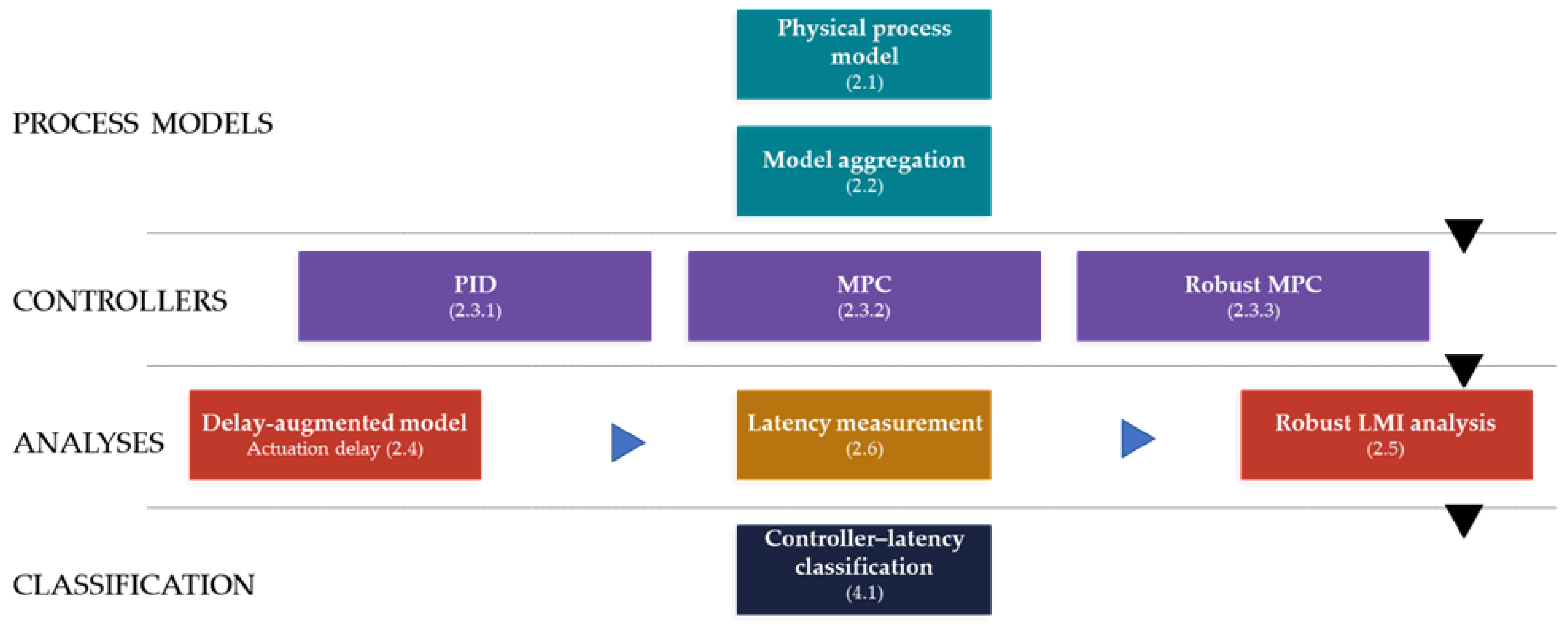
Figure 1 provides an overview of the methodology pipeline. The workflow is organized into four tiers: process modeling (Section 2.1 and Section 2.2), controller design (Section 2.3), analysis (Section 2.4, Section 2.5 and Section 2.6), and classification (Section 4.1). Solid arrows indicate the primary data flow; the three analysis components operate in parallel on the controller outputs and feed jointly into the final classification.

2.1. Physical Process and Finite-Difference Model

The physical system is a steel slab subject to a controlled heat flux at its front face (x = 0), modeling a laser or inductive heating scenario. Heat conduction through the thickness follows the one-dimensional diffusion equation. The thermal properties of steel are: thermal diffusivity α, volumetric heat capacity ρC_p, and thermal conductivity k_cond = α·ρC_p. The rear face (x = L) loses heat by convection to an ambient temperature T_amb with convection coefficient h.

The domain is discretized into N_x uniformly spaced nodes (dx = L/(N_x−1)). The finite-difference scheme is explicit with the time step:

$$dt={\displaystyle \frac{0.5\cdot d{x}^2}{\alpha }},$$

(1)

chosen to satisfy the von Neumann stability condition r = α·dt/dx² for all considered material scenarios. The resulting state-space update is:

$$T_{k+1}=A\cdot T_k+B\cdot u_k+b,$$

(2)

where T_k ∈ ℝ⁴¹ is the nodal temperature vector, u_k (W/m²) is the applied heat flux at x = 0, b ∈ ℝ⁴¹ is the affine offset from the convective boundary condition at x = L. Interior nodes follow a standard three-point finite-difference stencil; a ghost-node Neumann condition is applied at x = 0 and a Robin convective condition at x = L. Temperature is extracted at two measurement locations x₁ and x₂.

The maximum allowable heat flux is q_max, representative of laser-like irradiation. The 1D formulation is intentional: it isolates the computational feasibility question in a tractable linear setting; extension to higher-dimensional or nonlinear process models would increase state dimension and worsen MPC latency profiles, strengthening rather than weakening the classification presented.

2.2. Model Aggregation to Control Rate

The plant integration step dt is far shorter than the control period Δt_c, so an aggregated model is derived to enable MPC prediction matrices at the control rate.

In effect, this produces a single matrix equation that captures exactly what happens to the temperature field over one full control interval, allowing MPC to plan at the slower control rate without losing physical accuracy.

Given m = ⌈Δt_c/dt⌉ plant steps per control step:

$$\begin{gathered} \bar{A}=A^m, \\ \bar{B}={\sum }_{i=0}^{m-1}{A}^{i}B, \\ \bar{b}={\displaystyle \sum _{i=0}^{m-1}}{A}^{i}b \end{gathered}$$

(3)

The aggregated model $T_{k+1}=\bar{A}\hspace{0.17em}{T}_k+\bar{B}\hspace{0.17em}{u}_k+\bar{b}$ describes exactly the state transition over one control interval, enabling MPC prediction matrices to be built at the control rate. With the aggregated model in place, the three controller designs are now described.

2.3. Controller Designs

2.3.1. PID Control

A single-point PID controller regulates temperature at x = 0 mm (boundary), computed at every control step:

$$u_k={sat}_0^{q_{max}}\left(K_p{e}_k+K_i{\xi }_k-K_d{\dot{y}}_k\right),$$

(4)

Gains were tuned to _Kp and K_i with K_d = 0 and anti-windup back-calculation gain a_w. The integrator state ξ_k is updated only when the control signal is not hard-saturated. A two-point PID extension uses a weighted composite error.

2.3.2. MPC Receding Horizon

MPC minimizes a finite-horizon quadratic cost at every control step. Prediction matrices Φ, Γ, and S are constructed from the aggregated model in the standard receding-horizon formulation [20].

In plain terms, the MPC controller looks Np steps ahead, predicts the temperature evolution under different heat flux sequences, and selects the sequence that minimizes tracking error subject to the physical flux limit. This prediction and optimization is performed fresh at every control step, which is the source of its higher per-cycle computational cost compared to PID.

The optimization problem solved at each control step takes the form of a bounded quadratic programme:

$$\begin{gathered} \underset{U}{min}\hspace{0.33em}1/2U^{\top }HU+f^{\top }U \mathrm{s}.\mathrm{t}. 0\le U\le q_{max}, \\ H={\Gamma }^{\top }{Q}_{blk}\hspace{0.17em}\Gamma +R_u\hspace{0.17em}{I}_{N_p}, f={\Gamma }^{\top }{Q}_{blk}\left(\Phi \hspace{0.17em}{x}_0+S-Y_{ref}\right), \end{gathered}$$

(5)

with block output weight Q_blk = I_Np ⊗ Q_y. Box constraints are enforced directly. The QP is solved by OSQP [24] with warm-starting (eps_abs = eps_rel = 10⁻⁴, max_iter = 4000, adaptive_rho = 1, polish disabled) for the timing comparison study and by quadprog [25] (dense active-set) for the Robust MPC timing analysis. The prediction horizon is different between the timing comparison and the single-controller experiments.

2.3.3. Robust MPC

Robust MPC extends nominal MPC to a scenario set of nS = 3 uncertain models, each corresponding to a different combination of thermal properties:

For each scenario s, the aggregated model ($\bar{\mathrm{A}}$_s, $\bar{\mathrm{B}}$_s, $\bar{\mathrm{b}}$_s) and prediction matrices (Φ_s, Γ_s, S_s) are computed. The QP Hessian and gradient are formed as equal-weight averages over scenarios (w_s = 1/3):

$$\begin{gathered} H=R_u\hspace{0.17em}{I}_{N_p}+{\sum }_s{w}_s\hspace{0.17em}{\Gamma }_s^{\top }{Q}_{blk}\hspace{0.17em}{\Gamma }_s, \\ f=\sum _s{w}_s\hspace{0.17em}{\Gamma }_s^{\top }{Q}_{blk}\left({\Phi }_s\hspace{0.17em}{x}_0+S_s-Y_{ref}\right), \end{gathered}$$

(6)

The true plant in the simulation is scenario 2 (nominal). The same QP structure as nominal MPC applies, but H and f now aggregate information from all three models, making the control law implicitly robust to the parameter uncertainty set. In MPC_time1R, the QP is solved by quadprog with a full dense Hessian; in MPC_time2R, OSQP with a precomputed sparse Hessian and warm-starting is used. To analyse the effect of DT computation time on closed-loop behavior, the plant model is augmented with an explicit actuation delay.

2.4. Delay-Augmented Model for Actuation Delay Analysis

To model the situation where the DT computation itself introduces a delay before the calculated command reaches the actuator, the plant state is extended with a memory of past inputs—the controller sees the process evolving under a command that was computed d steps ago.

Actuation delay of d control steps is modeled by augmenting the plant state with a d-step input buffer. The PI integrator state is included in the augmented vector, and the most delayed input drives the plant at each step. For MPC, this augmented model is supplied directly to the prediction module so the controller plans over the true delay-affected dynamics. PI gains used in the delay analysis are specified in Section 2.7; actuation delay value d = 1, …, 5 control steps correspond to 10–50 ms. The delay-augmented model provides the closed-loop matrices needed for formal stability certification via linear matrix inequalities.

2.5. Robust LMI Delay-Margin Analysis

The LMI analysis asks a formal mathematical question: is there a single stability certificate—a Lyapunov function—that works simultaneously for all three uncertainty scenarios and for a given actuation delay? If such a certificate exists, the closed loop is guaranteed stable regardless of which scenario the true process corresponds to.

The maximum delay for which a common Lyapunov function certifies robust stability across all scenarios is found by solving a semidefinite feasibility problem at each candidate delay d. For each scenario s with closed-loop matrix Φ_s(d) (augmented for delay d), the condition:

$$P-{\Phi }_s{\left(d\right)}^{\top }P\hspace{0.17em}{\Phi }_s\left(d\right)\succ 0, \forall \hspace{0.17em}s\in \{1,2,3\},$$

(7)

is cast as a linear matrix inequality (LMI) in the symmetric positive-definite matrix P. This is solved using CVXR with the SCS solver [26]. A positive semidefinite auxiliary variable $Z_i=P-{\Phi }_s{\left(d\right)}^{\top }P\hspace{0.17em}{\Phi }_s\left(d\right)-\epsilon I, \epsilon ={10}^{-8}$ enforces strict feasibility. A delay scan is performed with step_d = 5 control steps up to d_max.

The finite-horizon robust induced gain γ_T(d) quantifies the worst-case output amplification over a horizon N_h as a function of actuation delay d, providing a complementary sensitivity measure to the binary LMI feasibility check. The final methodological component concerns how per-cycle computation time is measured and attributed to its constituent phases.

2.6. Latency Measurement

Per-cycle latency τ_k is measured as wall-clock time from the start of the control computation to the return of the control command, using platform-native high-resolution timers.

Latency is decomposed into: (i) build time—construction of H and f from the current state; (ii) QP solve time—the OSQP or quadprog solver call. For PID, the QP solve component is zero. The per-cycle deadline is set to Δt_c (strict equality with the control period), so a deadline miss occurs when τ_k > Δt_c. Analysis of the timing data confirms that QP solve time accounts for 99.1% of total latency variance in steady state, indicating that the operating system (OS) scheduler interference is a minor contributor for this configuration; the general-purpose OS deployment is nonetheless intentional, representing a worst-case baseline against which real-time kernel deployments can be compared.

Summary statistics computed for each controller: mean, p50, p90, p95, p99 (99th percentile latency), maximum latency; deadline miss count and rate; mean CPU utilization (mean(τ)/Δt_c). All implementations are in R version 4.4.2 (2024-10-31 ucrt) (version ≥ 4.3) using packages quadprog 1.5.8, osqp 0.6.3.3, Matrix 1.7.1, and CVXR 1.0.15. The results of applying this methodology across all controller types are presented in the following section.

2.7. Case Study and Parameter Values

The methodology described in Section 2.1, Section 2.2, Section 2.3, Section 2.4, Section 2.5 and Section 2.6 is general and applicable to any linear process model with bounded inputs. To make the analysis concrete and reproducible, all experiments in this paper are instantiated on a single case study: boundary heat flux control of a 1 mm steel slab to a 200 °C setpoint, representative of laser-based and induction heating processes in additive manufacturing and surface treatment. The parameter choices below reflect physically realistic values for steel under laser-like irradiation and are held fixed across all controller comparisons to ensure that latency differences are attributable to controller architecture rather than problem size or tuning.

Physical model: Nx = 41 nodes, α = 1.2 × 10⁻⁵ m²/s, ρCp = 3.8 × 10⁶ J/(m³·K), h = 100 W/(m²·K), qmax = 5 × 10⁷ W/m², Tamb = 22 °C, dt = 26 μs. Sensor positions x₁ = 0.2 mm and x₂ = 0.8 mm. For Δtc = 5 ms, m ≈ 192; for Δtc = 10 ms, m ≈ 384.

PID controller: Single-point gains Kp = 1 × 10⁵ W/(m²·°C), Ki = 5 × 10³ W/(m²·°C·s), Kd = 0, anti-windup gain aw = 0.2. Two-point extension uses weighted composite error e = 0.6·e₁ + 0.4·e₂, with gains Kp = 2 × 10⁴ W/(m²·°C) and Ki = 8 × 10² W/(m²·°C·s), updated every 100 plant steps (~2.6 ms).

MPC cost function: Qy = diag(1,1), Ru = 1 × 10⁻⁸, Yref = 1Np ⊗ [200, 200]ᵀ °C. Prediction horizon Np = 120 steps (1.2 s at Δtc = 10 ms) for the timing comparison and Np = 400 steps (2 s at Δtc = 5 ms) for the single-controller experiments.

Robust MPC: Equal scenario weights ws = 1/3. Uncertainty scenarios as defined in

Table 1. Uncertainty scenarios for Robust MPC and LMI analysis.

Parameter	Scenario 1	Scenario 2 (Nominal)	Scenario 3
α (m2/s)	0.8α0 = 9.6 × 10−6	1.2 × 10−5	1.2α0 = 1.44 × 10−5
ρCp (J/m3·K)	0.9ρCp0 = 3.42 × 106	3.8 × 106	1.1ρCp0 = 4.18 × 106
h (W/m2·K)	0.5h0 = 50	100	2.0h0 = 200

.

Delay analysis: PI gains Kp = 8 × 10⁵ W/(m²·°C), Ki = 2 × 10⁷ W/(m²·°C·s) with anti-windup; MPC horizon Np = 200 steps at Δtc = 10 ms.

LMI scan: Nh = 200 steps (T = 2 s), stepd = 5 control steps, dmax = 200 steps (2 s).

All computations are performed in R (version ≥ 4.3) on a standard desktop PC without real-time OS support, making the reported latencies conservative upper bounds relative to a dedicated real-time platform.

3. Results

3.1. Control Performance and Per-Controller Latency Analysis

All three controllers were tested for their performance (single-point PID control tracking a 200 °C, two-point PID controlling temperatures at x₁ = 0.2 mm and x₂ = 0.8 mm simultaneously, and MPC two-point tracking at Δt_c = 5 ms, Np = 400 steps). They successfully tracked the 200 °C setpoint; MPC additionally provides explicit constraint satisfaction on the heat flux u ∈ [0, 5 × 10⁷] W/m². 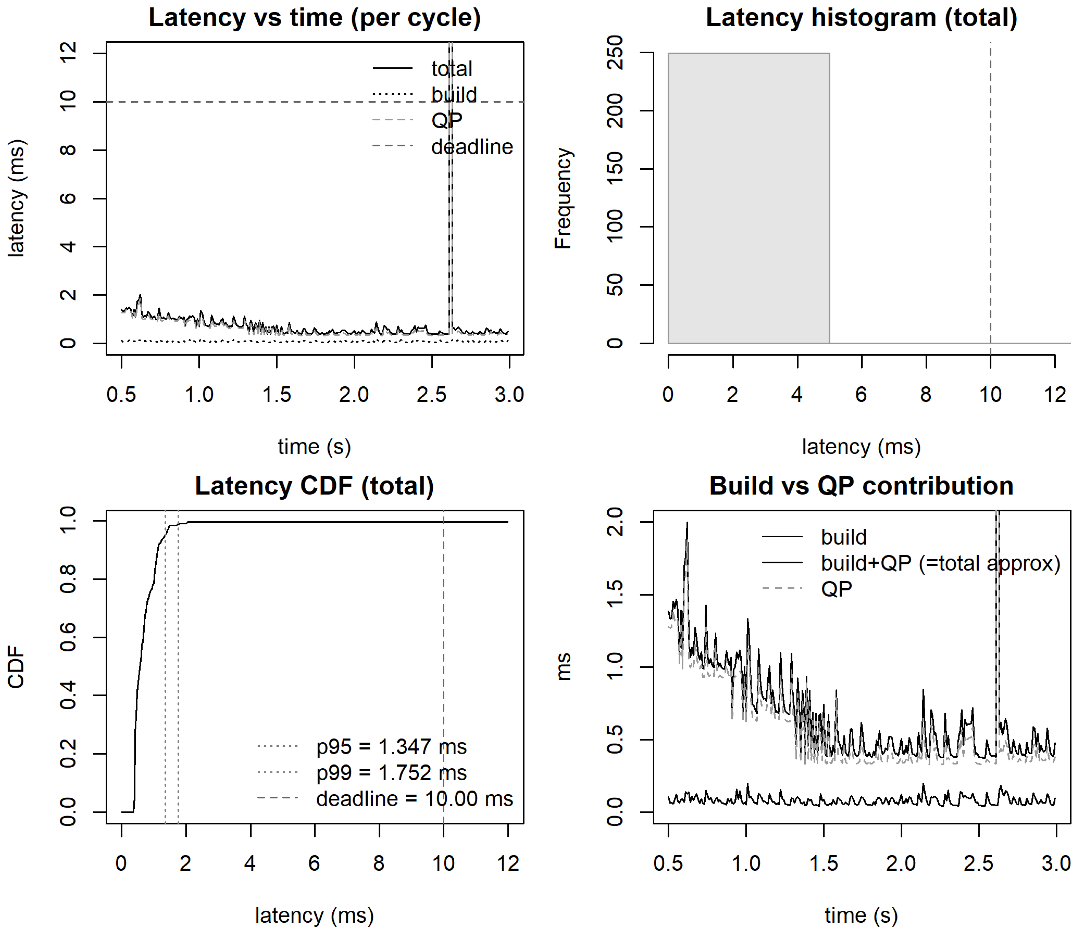In particular, Figure 2 shows the MPC per-cycle latency statistics (Np = 120, Δt_c = 10 ms, OSQP warm-start). The time series shows a transient settling within 0.5 s; the histogram is right-skewed with most cycles below 2 ms. The empirical CDF (bottom-left) confirms p95 = 1.347 ms and p99 = 1.752 ms, both within the 10 ms deadline. No deadline misses occur. The build-vs.-QP breakdown (bottom-right) shows that problem construction (linear-term update f = Mx₀ + c) dominates over the OSQP solve, indicating that the sparse precomputed Hessian strategy has shifted the bottleneck to matrix-vector products.

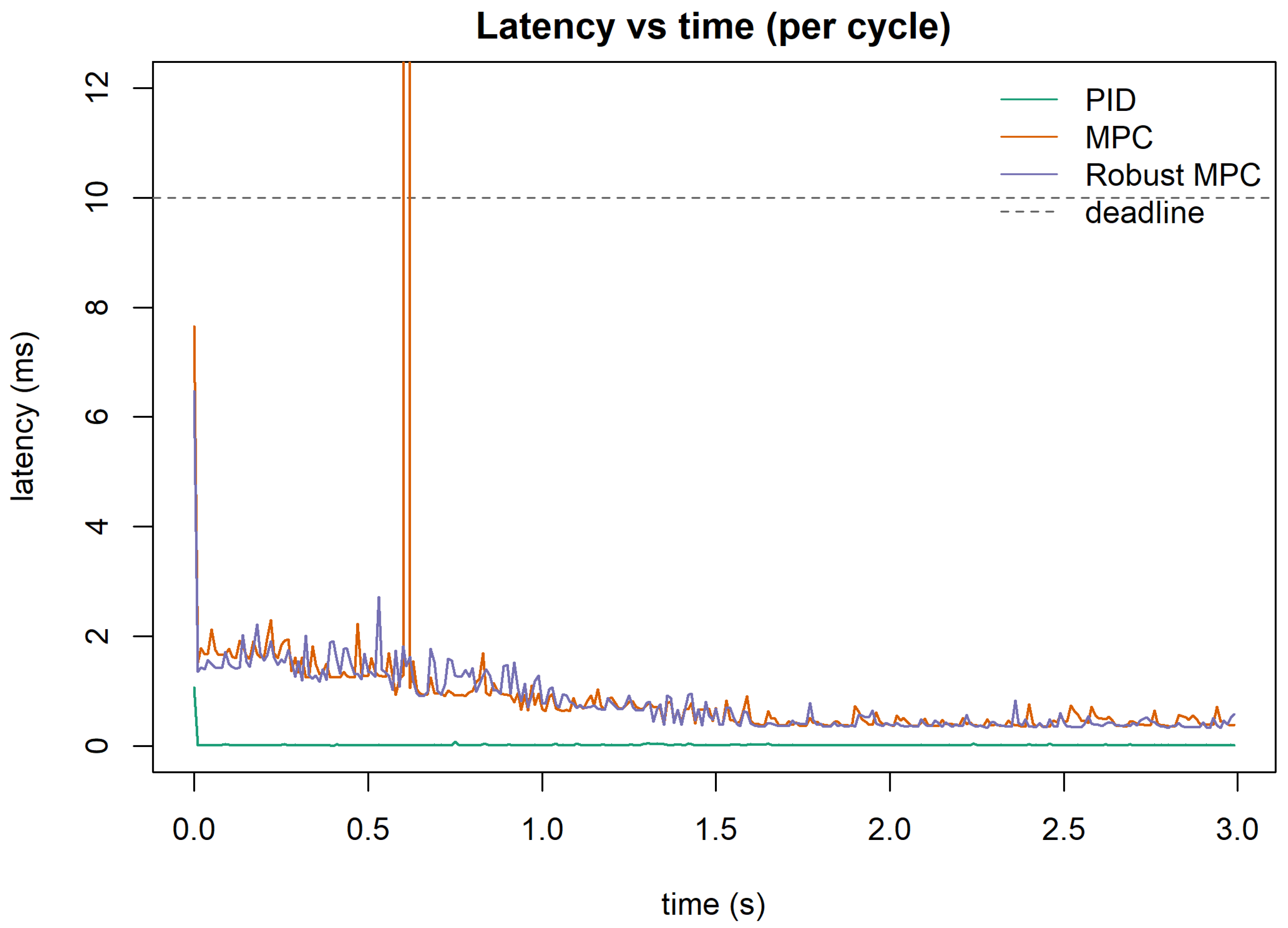
The relative latency of all three controllers is best appreciated by direct comparison. Figure 3 overlays per-cycle latency for all three controller types across a 3 s simulation. PID latency (teal) is indistinguishable from zero on this scale (<0.05 ms). MPC latency (orange) is 0.3–2 ms per cycle after the initial transient. Robust MPC latency (blue) is an order of magnitude higher, with frequent peaks exceeding 3 ms even during the transient period—noting that these are the values shown at the 10 ms control period scale; the actual Robust MPC results at the 5 ms period are shown separately in Figure 4.

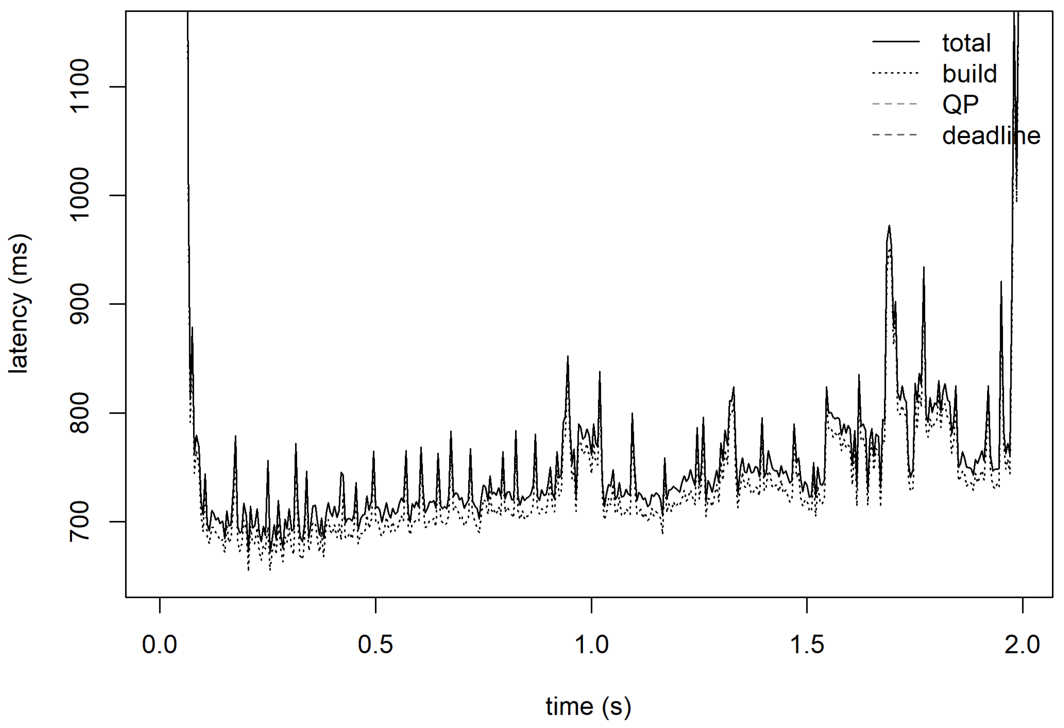
Figure 4 shows the full Robust MPC latency time series at Δt_c = 5 ms. Mean latency is 770.1 ms—a ratio of 154× relative to the 5 ms control period. The signal is dominated by the build phase (constructing the weighted-sum Hessian and gradient across nS = 3 scenarios, each with Γ ∈ ℝ^{800 × 400}), with the quadprog dense QP solve contributing a smaller but non-negligible fraction. Latency spikes exceed 1100 ms.

A direct validity question arises from the 154× latency ratio: if each QP solve takes 770 ms on average, how does the closed-loop simulation remain meaningful against a 5 ms control period? While the current QP solve runs, the plant integrates forward using the most recently computed command u_hold applied as a zero-order hold at the high plant rate. This is physically valid for the steel slab studied here: the thermal time constant (~0.3 s) is far longer than the computation latency, so the process state changes negligibly between control updates. For processes with faster dynamics, this assumption would not hold, and the near-real-time classification would translate directly into closed-loop instability rather than merely degraded tracking.

3.2. MPC Horizon Sensitivity

Having confirmed that all three controllers achieve their tracking objectives and characterized their base latency profiles, attention turns to MPC horizon sensitivity—the primary design parameter governing soft-real-time feasibility. MPC p99 latency was evaluated as a function of prediction horizon Np for single-scenario (nS = 1) and three-scenario (nS = 3) robust configurations. The reference τmax = 160 ms is the LQR-equivalent delay tolerance (the maximum delay after which a static LQR gain destabilizes the nominal closed loop). For all tested horizons (Np ∈ {75, 125, 175, 220}), p99 latency remains below 1.7 ms—well within both the 5 ms control period and the τ_max reference. The nS = 3 values are moderately higher than nS = 1, reflecting the larger f-update computation, but remain in the same order of magnitude.

3.3. Delay Robustness: PI vs. MPC

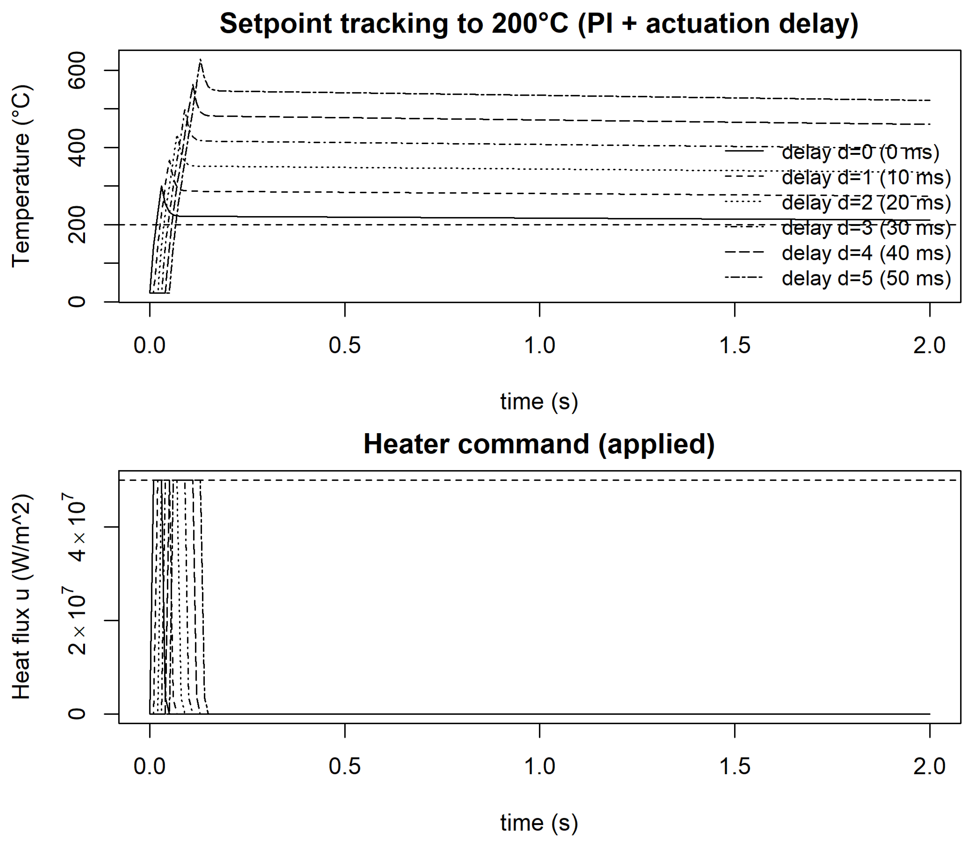
With latency feasibility established across all tested prediction horizons, the analysis now examines whether MPC’s per-cycle overhead translates into a compensatory benefit: explicit tolerance of actuation delay that simpler controllers cannot provide. Figure 5 shows PI closed-loop step responses for actuation delays d = 1–5 control steps (10–50 ms at Δt_c = 10 ms). At d = 1 (10 ms), tracking is stable with overshoot. At d = 3 (30 ms), the system reaches the stability boundary with sustained oscillation. At d = 4 and d = 5, PI control is unstable, with unbounded oscillations in both the temperature output and the heat flux command.

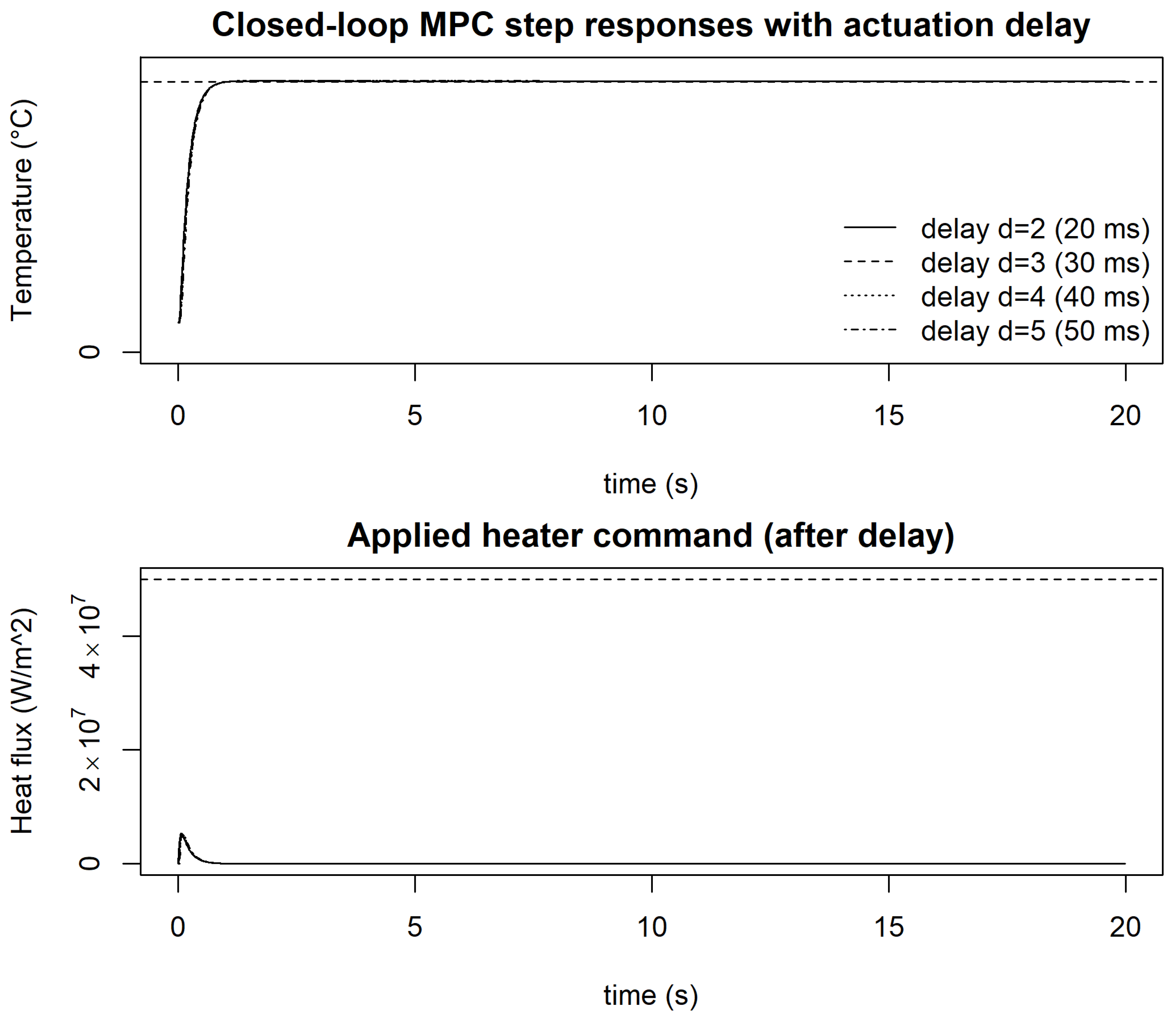
Figure 6 shows the corresponding MPC responses. MPC maintains stable tracking across the full delay range d = 2–5, with setpoint convergence in approximately 1 s for all delay values. This robustness arises because MPC incorporates the delay model explicitly in the augmented state (Section 2.4), allowing it to plan control sequences that compensate for the known lag.

Concerning the characterization of the latency distribution in the d = 5 scenario specifically: latency is concentrated around 75–120 ms with heavy-tailed spikes to 300 ms, and every cycle misses the 5 ms deadline.

3.4. Robust LMI Delay Margin and Induced-Gain Analysis

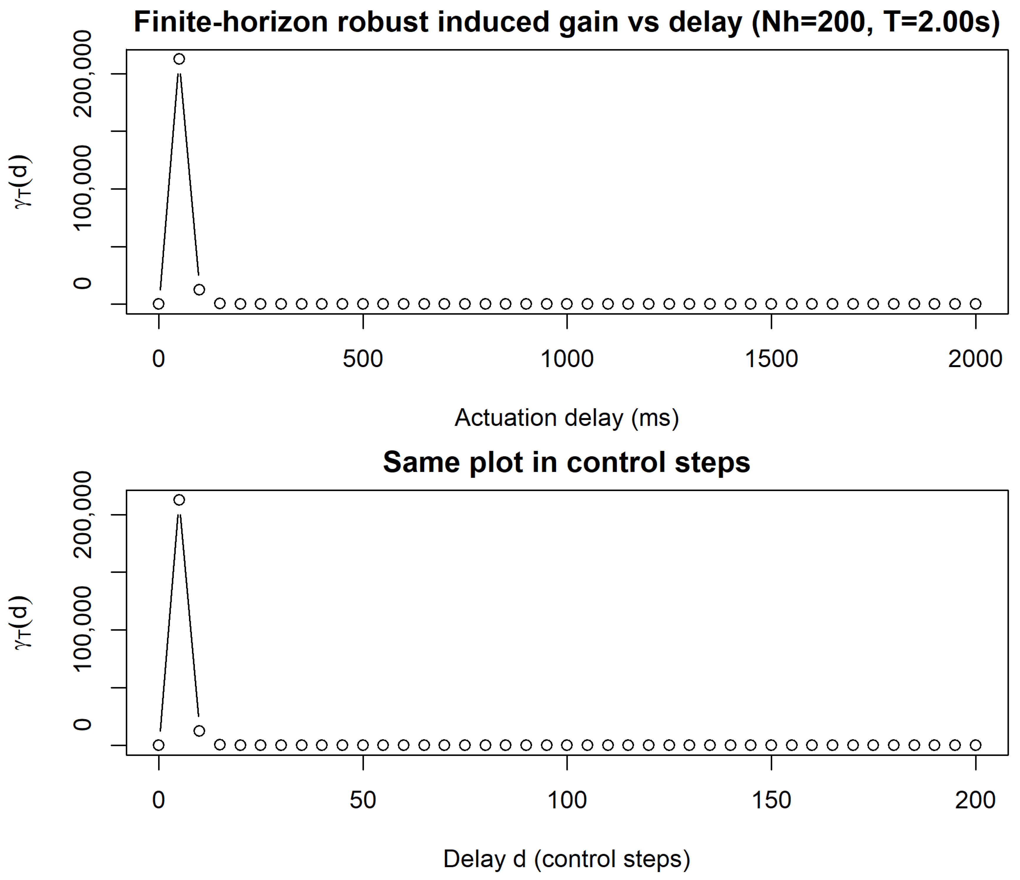
The delay-robustness comparison raises a formal question: up to what actuation delay can closed-loop stability be rigorously certified across the full uncertainty set, independently of simulation behavior? Figure 7 presents the finite-horizon robust induced gain γ_T(d) as a function of actuation delay d (in control steps, with Δt_c = 10 ms), computed over N_h = 200 control steps (T = 2 s). The gain is near zero for small delays, reaches a sharp maximum of approximately 175,000 at d ≈ 100 steps (1 s), and then decays to near zero for larger delays. The shape reflects the finite-horizon nature of the metric: for very short delays, the controller has sufficient authority to reject disturbances; for very long delays, the process settles before the delay acts significantly; the worst case is at intermediate delays where timing and system dynamics interact resonantly.

The LMI feasibility scan complements the induced-gain result with a binary stability certificate. It establishes the maximum certifiably stable delay d* by checking the existence of a common Lyapunov matrix P across all three uncertainty scenarios at each candidate delay. The scan uses step_d = 5 control steps up to d_max = 200 steps, and the SCS solver (via CVXR). The scan finds no infeasibility up to the tested bound of d = 200 steps (2 s), indicating that the closed-loop system with gain K is robustly stable for all actuation delays within the scanned range. The combined latency and stability results are now interpreted in terms of practical deployment implications.

4. Discussion

4.1. Controller–Latency Classification

Using the classification established in Section 1.2,

Table 2. Controller–latency classification and real-time deployment feasibility. Latency values are for Δt_c = 10 ms (PID, MPC) and 5 ms (Robust MPC) on standard desktop hardware, R implementation.

Controller	Mean Latency	p99 Latency	Deadline Misses	Offline Estimable?	RT Class
PID	<0.05 ms	<0.1 ms	None	Yes, once	Hard/Soft
MPC (OSQP warm)	~1 ms	2.426 ms	None (10 ms)	No	Soft
Robust MPC (Np = 400)	770 ms	>1000 ms	All (5 ms)	No	Near RT
Robust MPC (OSQP warm, Np = 120)	~1 ms	~1.7 ms	None (10 ms)	No	Soft

This table provides a direct mapping from controller choice and implementation to deployable real-time class; the Robust MPC classification depends critically on solver and horizon choice.

consolidates the real-time characteristics of each controller, providing a direct deployment decision framework for DT-based process control.

To assess whether the soft-real-time classification of nominal MPC generalizes beyond the 1D geometry, the timing experiment was repeated on a 2D finite-difference model of the same steel domain (21 × 21 nodes, n = 441 states, dx = dy = 50 μm). Per-cycle p99 latency was 2.216 ms—marginally below the 1D value of 2.426 ms—with zero deadline misses against the 10 ms deadline. The result confirms that nominal MPC latency is dominated by the QP solve (Np = 120 variables, independent of state dimension) rather than the build step, and the soft-real-time classification is therefore robust to state dimension increase. Robust MPC was not extended to 2D as its build step scales with n² across scenarios; based on the 1D measurements, latency would increase to the order of minutes, further reinforcing the near-real-time classification.

The classification in Table 2 raises an immediate practical question: how should a DT architect respond when the required controller falls in the near-real-time class?

4.2. Implications for DT Deployment

These latency results are broadly consistent with and extend the MPC benchmarking literature. Frison et al. [23] reported 2–8× speedups over state-of-the-art solvers using hardware-tailored linear algebra on embedded processors; the values reported here are higher due to R’s interpreted overhead, confirming that the latency floor could be reduced substantially in a production C/C++ implementation. Hartley et al. [22] achieved fast MPC cycles on FPGA for a 12-state aircraft model; the 41-state thermal model studied here would require proportionally more resources on equivalent hardware. Chen et al. [14] demonstrated that neural surrogate predictors reduce MPC computation toward near-real-time rates in additive manufacturing—a direction consistent with the near-real-time classification of Robust MPC reported here and with the surrogate-based future directions identified in Section 6. The key distinction of the present work is not the absolute latency values, which depend on implementation language and hardware, but the mapping of those values to DT real-time deployment classes with LMI-certified delay margins across an uncertainty set—a step absent from all prior benchmarking studies.

Despite its high latency, Robust MPC remains deployable through architectural adaptation. The 154× ratio for Robust MPC does not render it unusable—it redefines the deployment architecture. Three deployment options exist: (i) increase the effective control period to ~1 s; (ii) use a hierarchical architecture where Robust MPC sets reference trajectories for a lower-level PID or MPC; (iii) pre-compute the control law via explicit MPC or a neural operator surrogate [21,27].

A critical practical consequence of DT latency emerges from the delay-robustness results (Section 3.3): in DT architectures where computational latency is unavoidable, MPC provides inherent delay compensation that PI-based controllers do not. A DT running MPC can tolerate 50 ms actuation delays [20] (d = 5 at Δt_c = 10 ms) while maintaining stable tracking; a PI-controlled DT destabilizes beyond approximately 30 ms for this process. Wherever DT latency exceeds ~20–30 ms, MPC is the controller of choice, since the DT computation itself becomes the source of actuation delay (Section 3.3).

The induced-gain peak at d ≈ 100 steps (Figure 7) provides a further design constraint: there exists a worst-case delay around 1 s where disturbance amplification is maximized. DT architectures operating at or near this latency should be redesigned to shift above or below this peak, as the γ_T(d) curve decays to near zero for both very short and very long delays. These deployment implications are now placed in the broader context of Industry 4.0 and 5.0 manufacturing architectures.

4.3. Industry 4.0 and 5.0 Context

The results confirm that DT-based process control is computationally feasible for PID and standard MPC on general-purpose hardware (Industry 4.0 deployment) at soft-real-time rates. No real-time OS, dedicated DSP, or FPGA is required for Np ≤ 220 with OSQP warm-starting.

In the Industry 5.0 framing [28], the near-real-time classification of Robust MPC is consistent with its natural role as a decision-support layer rather than an autonomous fast controller. A human operator can supervise and override Robust MPC recommendations without violating the physical control loop, since the fast PI or MPC layer handles the immediate dynamics. This positions Robust MPC as a human-centric planning tool within a hierarchical DT architecture—computing safe, uncertainty-aware reference trajectories that the lower layer tracks in real time.

The LMI delay-margin analysis provides a formal basis for DT certification in safety-relevant contexts: for a given uncertainty set and controller gain, d* gives the maximum delay that the DT communication and computation pipeline may accumulate before closed-loop stability can no longer be guaranteed.

5. Conclusions

This study establishes a quantitative link between controller computational cost and achievable real-time performance in DT-based control. It has characterized the computational latency of PID, MPC, and Robust MPC controllers embedded in a digital twin for a 1 mm steel thermal process, quantifying their feasibility across hard, soft, and near-real-time categories. The main findings are as follows:

• PID computation is negligible (<0.05 ms) and satisfies hard-real-time constraints on standard hardware.
• Nominal MPC with OSQP warm-starting satisfies soft-real-time constraints (p99 < 2.5 ms) against a 10 ms deadline across all tested prediction horizons up to Np = 220 steps. Problem construction dominates over the QP solve; the sparse pre-computed Hessian strategy is the primary enabler. Latency measurements were obtained on a general-purpose OS; while QP computation dominates observed variance (99.1% in steady state), heavier system load could introduce additional scheduler-driven jitter not captured here.
• Robust MPC (nS = 3 scenarios, Np = 400, dense quadprog) exhibits mean latency of 770 ms (154× the 5 ms control period), classifying it as near real-time in this configuration. When OSQP warm-starting is used at Np = 120 (as in the horizon sensitivity study), Robust MPC p99 latency falls to approximately 1.7 ms, within the soft-real-time class. The classification is therefore implementation-dependent: dense QP at long horizons forces near real-time; sparse warm-started QP at moderate horizons achieves soft real-time even for the robust variant.
• MPC tolerates 50 ms actuation delays where PI destabilizes above ~30 ms.
• The LMI delay-margin analysis provides certifiable stability bounds for the full uncertainty set, and the induced-gain metric γ_T(d) reveals a worst-case sensitivity peak at d ≈ 100 control steps (1 s), informing architectural constraints on DT latency budgets.

The following limitations should be noted. The physical model is one-dimensional and linear, which may not capture processes with significant lateral heat flow or nonlinear material behavior; however, the 2D timing experiment confirms that the soft-real-time classification of nominal MPC is robust to state dimension increase. Latency measurements were performed on a general-purpose OS in R; production implementations in C/C++ on a real-time kernel would yield lower and more deterministic values. The uncertainty set for Robust MPC comprises three discrete scenarios; a continuous parameter uncertainty polytope might alter the LMI feasibility boundary. Finally, the LMI stability certificate uses a static gain K for the delay scan; extending this to the full receding-horizon MPC gain would require a parameter-dependent Lyapunov approach. These limitations directly motivate the future directions outlined in Section 6, including extension to nonlinear and multi-input processes, deployment on real-time kernels, continuous uncertainty polytopes, and parameter-dependent Lyapunov formulations.

6. Future Outlook

Several directions extend the present work. First, surrogate-based and explicit MPC formulations [29]—multi-parametric QP, DeepONet operator surrogates, or neural network approximators—should be benchmarked against online Robust MPC to quantify achievable latency reduction under pre-computation. Second, the analysis should extend to multi-input multi-output processes where the state dimension increases substantially. Third, deployment on real-time OS kernels (Xenomai, PREEMPT-RT Linux) or FPGA co-processors would provide deterministic latency bounds, enabling formal hard-real-time certification of MPC. Fourth, the delay-margin results motivate investigation of delay-compensating MPC formulations for DTs operating over cloud or wide-area networks with stochastic latency. Fifth, the integration of the controller-latency classification framework with DT orchestration middleware—enabling dynamic controller tier reconfiguration based on available compute—represents a practical step toward adaptive real-time DTs in Industry 5.0 environments.