Article

An Improved Random Forest-Based RUL Prediction Method for Elastic Supports with Vibration Signal Analysis


1
School of Computer Science and Technology, North University of China, Taiyuan 030051, China
2
School of Mechanical Engineering, North University of China, Taiyuan 030051, China
3
School of Mechanical and Electrcal Engineering, North University of China, Taiyuan 030051, China
*
Author to whom correspondence should be addressed.
Machines 2026, 14(5), 547; https://doi.org/10.3390/machines14050547
Submission received: 8 April 2026 / Revised: 2 May 2026 / Accepted: 11 May 2026 / Published: 14 May 2026
(This article belongs to the Section Machines Testing and Maintenance)

Abstract

As core vibration-damping components in rail transportation and aerospace, elastic supports are vital to equipment operational safety and maintenance cost control. Addressing the offline cumbersomeness and insufficient accuracy of traditional methods, as well as the poor adaptability of existing models to nonlinear damage and small samples, this study proposes a high-precision life prediction method based on a self-constructed full-life dataset and optimized random forest (RF). A self-developed triaxial vibration test bench was used to conduct accelerated aging tests on rubber–metal composite elastic supports, constructing a unique full-life dataset (412 valid samples) by collecting vibration signals via accelerometers and eddy current sensors. After extracting features like acceleration RMS and natural frequency, core damage-sensitive features were screened through PCA and Pearson correlation coefficients. The RF was optimized with a time-decaying factor and feature and parameter joint optimization to capture temporal degradation and resist overfitting. Experimental results show that the model achieves RMSE = 0.026 and R2 = 0.988, significantly outperforming Gray Prediction, BP Neural Network, and XGBoost. It accurately captures the life evolution law of elastic supports, providing reliable technical support for online life prediction and predictive maintenance.

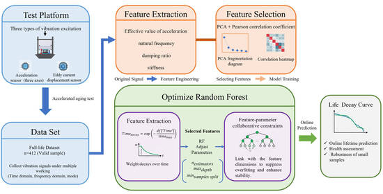
Graphical Abstract

1. Introduction

Elastic supports serve as the core vibration-damping and load-bearing components in mechanical equipment, finding extensive applications across critical fields such as rail transit, aerospace, construction machinery, and the automotive industry [1,2]. In the aerospace sector, they provide stable support for precision components (e.g., engine suspensions and avionics modules) under extreme conditions, such as high-altitude low pressure, rapid temperature changes, and intense mechanical vibrations, ensuring the reliable operation of key systems [3,4]. In construction machinery, they absorb vibration energy and reduce operational noise, thereby delaying structural fatigue damage and extending the overall service life of equipment [5,6]. However, elastic supports are subjected to multiple effects, such as alternating loads, temperature changes, and friction and wear over long periods, making them prone to material fatigue, stiffness degradation, and structural damage [7]. Failure to timely and accurately predict their remaining useful life (RUL) may lead to sudden equipment downtime, production interruptions, or even catastrophic safety accidents, resulting in significant economic losses and potential casualties [8]. Therefore, conducting research on the precise prediction of the remaining life of elastic supports is of great engineering value and practical significance for achieving predictive maintenance of equipment, reducing maintenance costs, and ensuring the stable operation of systems [9].
Traditional life prediction methods for elastic supports mainly rely on offline destructive testing and empirical formula fitting, which have inherent limitations that are difficult to overcome [10]. Offline destructive testing requires disassembling the support components from the equipment and conducting professional fatigue tests in laboratories, a process that is not only cumbersome and time-consuming but also fails to capture the dynamic evolution of damage during actual service [11]. This leads to significant deviations between predicted results and real service life, resulting in insufficient timeliness and accuracy in maintenance decisions. Empirical formulas, which are derived by fitting limited experimental data, often ignore individual differences in component materials, structural variations, and dynamic changes in service environments (e.g., load fluctuations and temperature variations), leading to poor generalization ability and difficulty in meeting the requirements of engineering practice [12]. To compensate for the shortcomings of traditional methods, Smalakys et al. developed a framework for extrapolating the laser damage fatigue life of optical materials based on Bayesian statistics and Markov Chain Monte Carlo (MCMC) techniques, combined with offline inspection scenarios, in order to improve the accuracy of life prediction [13]. However, this method still relies on offline data collection and is therefore not suitable for real-time online prediction of elastic supports in complex service environments. With the rapid development of industrial intelligence and the increasing demand for efficient operation, traditional offline prediction methods can no longer meet the needs of online monitoring and real-time early warning of key components. Therefore, developing a precise, efficient, and real-time RUL prediction technology based on in-service data has become an urgent research task in the field of equipment prognostics and health management (PHM) [14,15].
In recent years, advances in sensing technology, signal processing and machine learning have promoted the life prediction method based on vibration signals to become a research hotspot [16]. Vibration signals contain rich information about the health status of components. When material fatigue, stiffness attenuation or structural damage occur in elastic supports, their dynamic characteristics, such as natural frequency and damping ratio, change significantly, which is reflected in the time domain and frequency domain characteristics of vibration signals [17]. Minhee et al. proposed a novel sensor selection framework that adaptively selects vibration signals to improve the accuracy of service life prediction [18]. Li et al. developed an RUL prediction method based on multi-sensor data fusion, interpreting multi-sensor signals as proxies for inherent system degradation processes to predict remaining service life [19]. Regarding machine learning approaches, Zhang et al. proposed a bearing CV value assessment method based on cumulative Gray Prediction. By employing maximum likelihood estimation and SPSS analysis for failure simulation, they ultimately achieved high predictive accuracy [20]. However, in existing research, Gray Prediction methods are difficult to adapt to nonlinear degradation under complex working conditions, whereas BP Neural Network are prone to overfitting with small samples and have limited generalization ability [21,22]. These limitations make traditional machine learning methods difficult to meet the practical engineering requirements of high-precision and robust life prediction for elastic supports.
Full-life testing of elastic support components is characterized by high costs, long cycles, and significant resource consumption [23]. In practical engineering scenarios, researchers often encounter situations with limited sample data, which places greater demands on the robustness of predictive models and the efficiency of data utilization. As an ensemble learning method, random forest reduces the risk of overfitting through random sampling and feature selection and has good adaptability to high-dimensional data and small-sample scenarios. It has been verified in the life prediction of bearings, gears and other components [24,25]. Compared to deep learning models that rely on large-scale data training, random forests demonstrate unique advantages by uncovering latent correlations between features and lifespan within limited samples without requiring complex parameter tuning. Liu et al. proposed a rubber fatigue life prediction model based on the random forest algorithm [26]. This model uses strain amplitude, mean strain, and strain ratio as input variables, with rubber fatigue life as the output variable. By comparing the proposed model with the rubber fatigue life prediction model established by WANG et al., it is found that the prediction accuracy of the rubber fatigue life prediction model based on the random forest algorithm is higher [27]. However, the standard random forest still does not fully consider the temporal degradation characteristics of elastic supports, and the balance between feature dimension and model complexity under small-sample conditions still needs to be optimized [28]. Therefore, this paper makes targeted improvements to the random forest to improve the accuracy of life prediction.
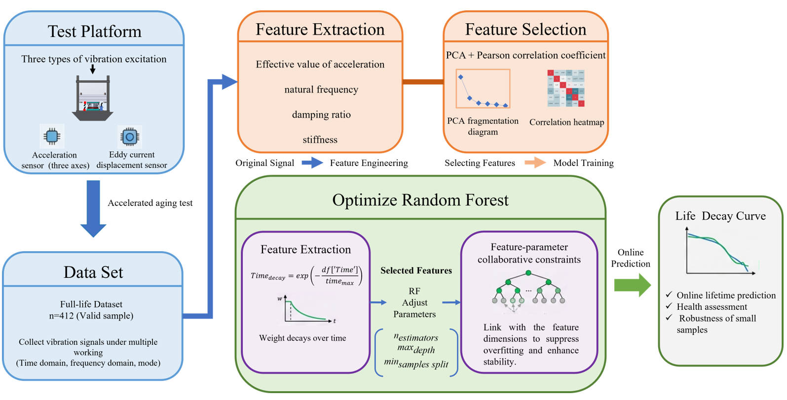
To address the aforementioned challenges, this study focuses on rubber–metal composite elastic supports and establishes a comprehensive technical framework encompassing “signal acquisition–feature extraction–feature screening–life prediction” (Figure 1). The specific research methodology is as follows: (1) Design a full-life accelerated aging test platform and use triaxial accelerometers and eddy current displacement sensors to collect vibration signals and relative displacement signals of elastic supports at different degradation stages. (2) Extract multi-domain feature parameters from the collected signals, including time domain features (acceleration RMS), frequency domain features (natural frequency and harmonic components), and dynamic mechanical features (damping ratio and dynamic stiffness). (3) Adopt a joint feature screening strategy combining Principal Component Analysis (PCA) and Pearson correlation coefficient analysis, where PCA is used to reduce the dimensionality of high-dimensional features and eliminate redundant information, while Pearson correlation analysis is used to select features strongly correlated with the degradation state, thereby obtaining a set of core damage-sensitive features. (4) Construct an improved RF life prediction model by introducing a time decay factor and a feature–parameter synergistic constraint system, and input the integrated core features and operational duration to realize precise prediction of the RUL of elastic supports. This framework effectively addresses the key issues of poor adaptability of traditional models to nonlinear damage and small-sample data, and provides a technical solution for the online life prediction of elastic supports.

2. Materials and Methods

2.1. Principal Component Analysis (PCA)

Principal Component Analysis (PCA), a classical and efficient data dimensionality reduction and feature extraction technique, is used to uncover inherent data structures, simplify complexity, eliminate redundancy, mitigate multicollinearity, and facilitate data visualization [29]. To address the high dimensionality and coupling of vibration signals, PCA extracts core features to reduce model complexity. This approach preserves essential information while significantly enhancing training efficiency and generalization [30].
The specific steps of Principal Component Analysis are:
First, the above features are standardized to unify their dimensions and numerical ranges. Based on normalized elastic support vibration characteristic matrix X R n × p ( n is the number of samples and p is the number of features).
Construct the covariance matrix R for the vibration dataset:
R = r 11 r 12 r 1 p r 22 r 22 r 2 p r p 1 r p 2 r pp ,
where r i j = l n l k = l n X k i X i ¯ X k j X j ¯ = l n l k = l n X k i X k j .
Subsequently, the covariance matrix R is eigendecomposed to obtain eigenvalues λ and their corresponding eigenvectors α. Larger eigenvalues indicate greater explanatory power, while eigenvectors define the feature weights for each principal component. To reduce the data dimensionality to k   ( k < n ) , we select the top components whose cumulative contribution rate exceeds a predefined threshold (typically 85–95%), ensuring the preservation of core data information. The formulas for single and cumulative contribution rates are given by:
C o n t r i b u t i o n   R a t e = λ 1 Σ k 1 p λ k k   =   1 , 2 , , p ,
C u m u l a t i v e   C o n t r i b u t i o n   R a t e = Σ k 1 i λ k Σ k 1 j λ k k = 1 , 2 , , p ,
Finally, the loading coefficients are calculated to identify key principal components. A higher absolute value signifies a stronger correlation between a feature and its corresponding principal component. The calculation formula is as follows:
a i j = α i j × λ i ,
To mitigate high-dimensionality and redundancy, PCA was applied to extract core features from vibration data, including RMS, frequencies, and stiffness. This dimensionality reduction optimized the data structure and strengthened the feature–lifespan correlations, facilitating robust predictive performance in the random forest model.

2.2. Random Forest Optimization Algorithm

2.2.1. Construction Process of the Traditional Random Forest

The construction of a traditional random forest mainly includes four key steps, which cooperate with each other to ensure the stability and prediction performance of the model [31]:
The first step is Bootstrap sampling. From the original dataset of size N, we use a random sampling Kmethod with replacement to generate N distinct subsets. Each subset contains approximately 63.2% of the original samples, while the remaining 36.8% serve as out-of-bag samples, which can be directly used for model evaluation, thereby improving data utilization efficiency.
The second step is random selection. During node splitting, random feature selection is implemented by sampling m candidate features from M features (Regression tasks: m = M/3). This mechanism effectively reduces model variance and enhances generalization ability by limiting the number of features during splitting.
The third step involves training the base decision trees. The regression tree was used as the base learner (CART), and each subset was trained independently [32]. The training process is based on a greedy algorithm that recursively splits the nodes, with the optimal split point selected with the goal of minimizing impurity until the termination condition is satisfied.
The fourth step is prediction result integration. For the regression task, this study “adopts the mean ensemble strategy” to summarize the prediction results of all base learners. This strategy effectively improves the overall prediction accuracy and operation stability of the model by balancing the prediction bias of a single decision tree.

2.2.2. Improved Random Forest Model

Traditional random forest models for life prediction often suffer from non-physical results in small-sample scenarios due to a lack of physical constraints and failure to account for time-series degradation [33]. This study addresses two key limitations: the inadequate modeling of vibration decay under alternating loads and the tendency toward overfitting and dimensionality explosion in data-constrained, long-term fatigue environments [34].
To address the limitations of purely data-driven models, which often yield non-physical results in small-sample fatigue assessments, this study proposes an improved random forest framework (Figure 2) that integrates physical degradation mechanisms directly into its internal learning architecture. Departing from conventional methods that treat time decay merely as an additional input, this approach constructs a time-attenuation factor based on the physical laws of stiffness degradation and damage accumulation to quantify aging trends. This factor is subsequently incorporated as a weight constraint within the decision tree’s node splitting criteria and ensemble voting mechanism, while a parameter-constrained optimization strategy is employed to eliminate redundant features and refine the feature space. By embedding these physical priors into the core training process, the model aligns with actual degradation mechanisms, shifting from a purely empirical approach to a robust, physics-informed learning framework. The implementation steps are detailed below:
First, introduce a time decay factor. To quantify the impact of the time dimension on lifespan prediction, define the time decay factor:
T i m e d e c a y = e x p ( t i m e a c t t i m e m a x ) ,
Here, t i m e a c t represents the actual operating time of the elastic support components, and t i m e m a x denotes the maximum operating time within the sample set. This factor takes values in the range (0, 1] and decreases as runtime increases. Incorporating it into the feature parameters enhances the model’s ability to capture long-term decay trends.
Second, establish a feature–parameter collaborative constraint system. For feature processing, implement a dynamic control strategy based on the sample–feature ratios. Aiming at the problem of overfitting in small samples, this paper uses physical information constraints to replace empirical feature restrictions and integrates physical laws, such as stiffness attenuation and natural frequency decline, into the model to avoid non-physical predictions. Feature optimization and parameter constraints are used to improve prediction rigor. For categorical features, adopt a “merge–encode–split–reduce” one-hot encoding strategy to keep categories under five. Additionally, construct polynomial interaction terms for key features (e.g., acceleration effective values and natural frequencies) to enhance nonlinear relationship modeling.
Given the small sample size characteristic of the dataset, this study adopted a conservative configuration strategy during the model parameter design stage by limiting the maximum depth of the decision tree to 15, increasing the node splitting threshold and the minimum number of samples in leaf nodes, and disabling Bootstrap sampling to fully utilize the limited sample data. At the same time, the Randomized Search CV method was used for parameter optimization, with specific settings of 12 iterations and threefold cross-validation. The final optimal parameter combination achieves a dynamic balance between feature dimensionality and model complexity, effectively mitigating dimensionality explosion and overfitting issues caused by small sample sizes.
The improved algorithm effectively improves the accuracy and robustness of life prediction under small-sample conditions by time dimension fusion and feature–parameter collaborative constraints.

2.2.3. Optimizing the Model Prediction Process

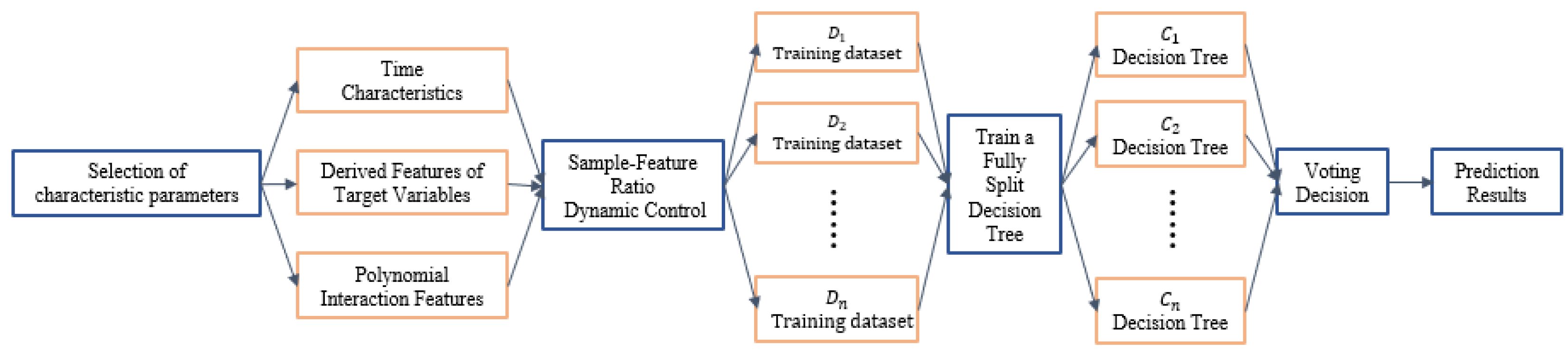
The training and prediction processes of the improved random forest are closely integrated with the aforementioned optimization strategies (see Figure 3). The specific implementation steps are as follows:
Step 1: Data preprocessing and feature screening. First, the collected vibration signal feature parameters (seven initial features, including #3 acceleration RMS, natural frequency, and damping ratio) are preprocessed: (1) Outlier removal: Due to the inherent resistance of the later random forest to a small number of outliers, it completely retains the key information of the later failure evolution. (2) Missing value processing: The dataset has a missing rate of 0.3%, and the mean value filling method is used to supplement missing values to ensure data integrity. Then, the PCA method is used to screen core features. The seven initial features are standardized, the covariance matrix is constructed, and eigenvalue decomposition is performed. Finally, three core principal components with a cumulative contribution rate of 92.3% are selected to eliminate redundant information.
Step 2: Feature fusion and training set construction. Introduce the time decay factor calculated by Formula (6) and fuse it with the three core principal components selected by PCA and the constructed polynomial interaction features (four second-order interaction terms and two third-order interaction terms) to form the final training feature set (total 3 + 1 + 4 + 2 = 10 features). The feature fusion process effectively integrates linear core features, nonlinear temporal features, and synergistic interaction features, providing a comprehensive data foundation for model training.
Step 3: Hyperparameter optimization. According to the feature–parameter collaborative constraint framework, define the hyperparameter search space: (1) number of decision trees ( n e s t i m a t o r s ): 50, 100, 150, and 200; (2) maximum tree depth ( m a x d e p t h ): 5, 8, 10, 12, and 15; (3) minimum number of samples for node splitting ( m i n s a m p l e s _ s p l i t ): 2, 3, 5, 8, and 10. Using Randomized Search CV, threefold cross-validation and twelve iterations of optimization are conducted to determine the optimal parameter combination ( n e s t i m a t o r s = 100 , m a x d e p t h = 10 , m i n s a m p l e s _ s p l i t = 5), which balances model complexity and prediction accuracy.
Step 4: Base tree training. Based on the optimal parameter combination, multiple independent CART decision trees are constructed. During the training process, Bootstrap sampling is disabled to fully utilize the limited 412 groups of sample dat. At each node splitting stage, three candidate features are randomly selected from the ten fused features (adjusted from m = M / 3 ) to reduce the correlation among the base trees. The nodes are recursively split according to the optimal split criterion (minimum MSE), and the splitting stops when the node sample size is less than five or the tree depth reaches ten.
Step 5: Prediction result integration. For the test set data, each base CART decision tree outputs an independent prediction result. The mean ensemble method is used to aggregate the prediction results of 100 base trees, and the average value is taken as the final RUL prediction result of the improved random forest model.
This improved approach not only retains the inherent advantages of random forests (strong noise resistance and high efficiency in handling high-dimensional data) but also effectively accommodates the time dependency of lifespan data and the small-sample characteristics of the dataset. Through multi-level feature fusion and parameter constraint optimization, it significantly improves the prediction accuracy and stability of the model, providing a reliable technical solution for the online lifespan prediction of elastic supports in engineering practice.

3. Experimental Results and Analysis

3.1. Introduction to the Dataset

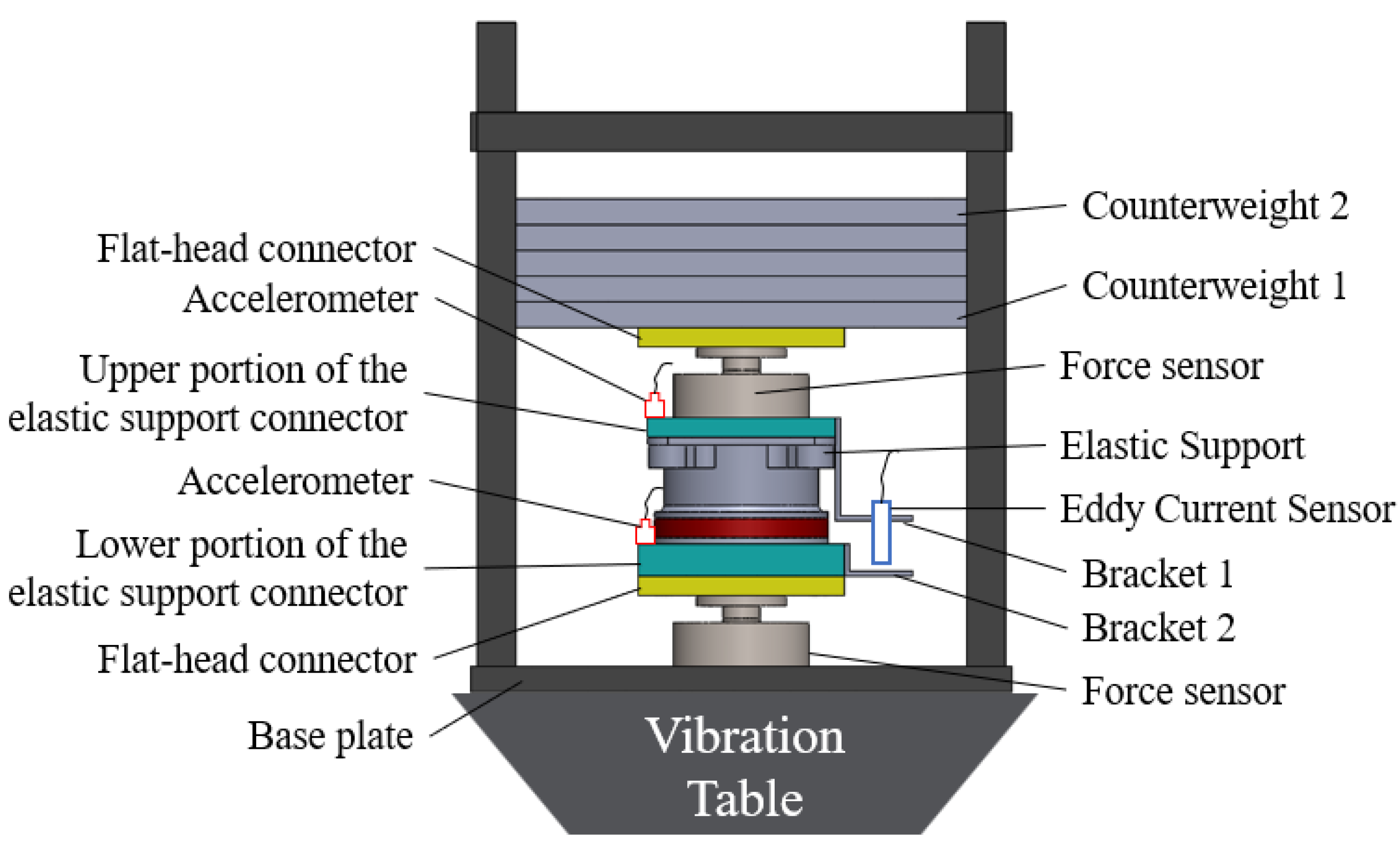
This study’s dataset originates from full-life accelerated aging tests conducted on elastic supports using a self-developed three-axis vibration test bench (as shown in Figure 4). The test subjects comprised three rubber–metal composite elastic support samples (designated as 2025030008, 2025030005, and 2025030002). The test design and data acquisition strictly adhered to engineering measurement standards, ensuring outstanding data integrity and reliability.
The test system is configured with eight equal-mass weights (approximately 25 kg each). The environmental test chamber is set to a constant temperature of 80 °C. After temperature stabilization, a preset vibration spectrum is applied at a fixed sampling frequency of 10,000 Hz. The sensing system comprises two IEPE-type vibration accelerometers (Model 1A347E) and one eddy current relative displacement sensor (Model IL-S025). The accelerometers were magnetically and adhesively secured to the upper and lower flanges of the elastic support to capture vibration acceleration signals. The eddy current sensor was mounted on the upper flange via a dedicated fixture, while a corresponding metal plate was installed on the lower flange to generate an eddy current field. This configuration enabled precise measurement of relative displacement between the upper and lower metal components. The structure of the test apparatus and the sensor layout are shown in Figure 4.
The sampling strategies for the three samples were designed with distinct data volumes to verify the model’s generalization ability under different sample sizes: (1) Sample 2025030008: “10 s sampling every 5 min”, total test duration of 6.2 h, collecting 74 groups of valid data (small-sample set); (2) Sample 2025030005: “10 s sampling every 5 min”, total test duration of 31.6 h, collecting 379 groups of valid data (medium-sample set); and (3) Sample 2025030002: “20 s sampling every 5 min”, total test duration of 34.3 h, collecting 412 groups of valid data (large-sample set). Each group of data included two channels of acceleration signals, one channel of displacement signals, and the corresponding time stamps and environmental temperature data. To ensure the adequacy of model training and validation, this study selected the largest dataset (sample 2025030002) as the core prediction data, while the other two datasets were used for supplementary verification of the model’s generalization performance.
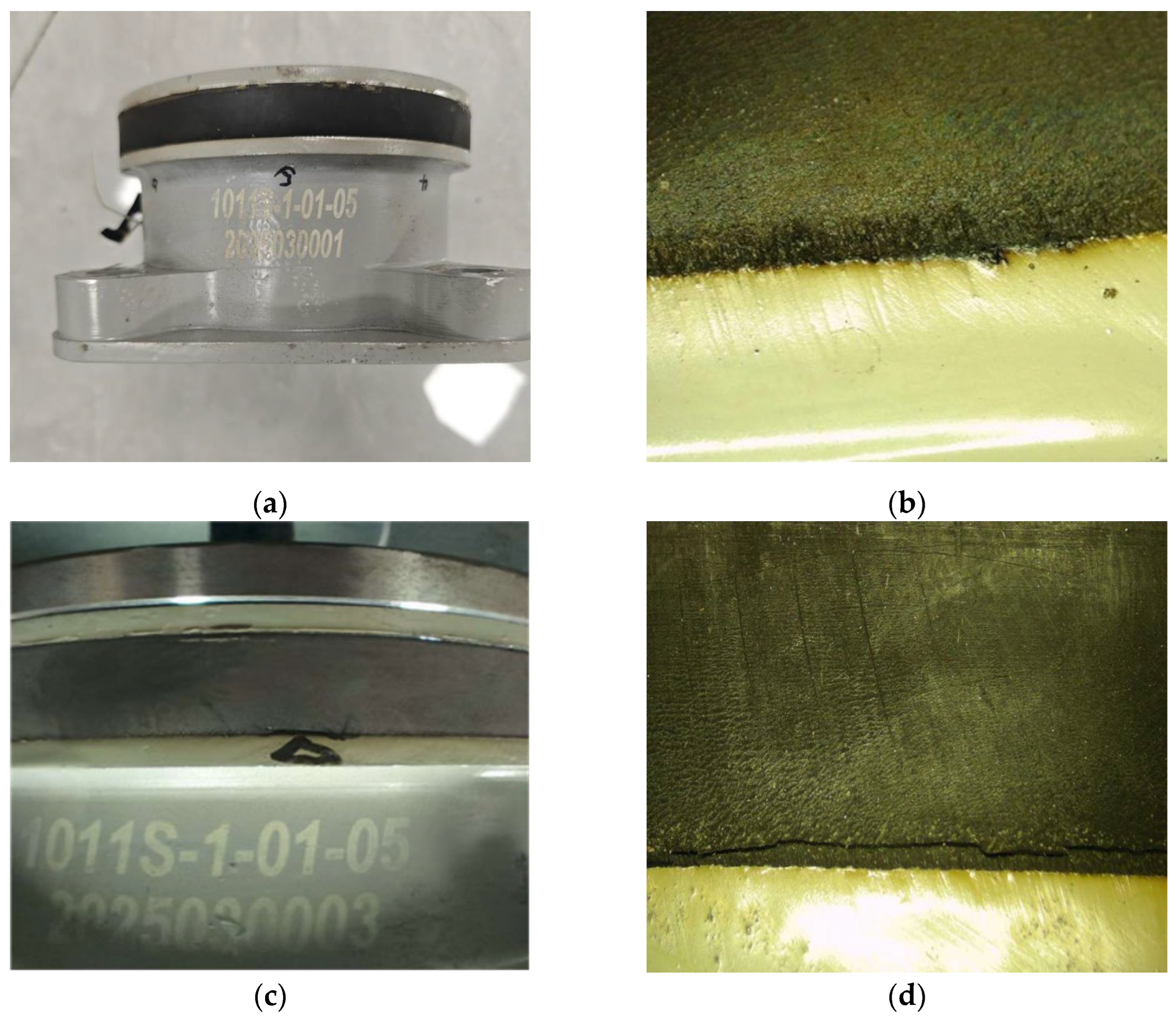
To define the quantitative endpoint of the elastic support RUL, this study only used physical damage as the sole criterion for defining the complete failure state (RUL = 0). This was verified by three full-life test samples. When the rubber layer appears through the radial crack, the metal–rubber interface is completely stripped, and the support loses its load-bearing and vibration isolation abilities, which is judged as failure, corresponding to Figure 5d. The RUL ranges of each stage in Figure 5 are: initial state (a), RUL = 100%; early damage (b), RUL= 60–80%; middle damage (c), RUL= 20–60%; and complete failure (d), RUL = 0. The dataset construction takes the physical failure time as the end of life, while the RUL values at intermediate sampling points were calculated by linear interpolation over the time intervals to ensure accurate and unified labeling.

3.2. Experimental Setup

3.2.1. Model Parameter Optimization

The core parameters of the random forest model include the number of decision trees ( n e s t i m a t o r s ), maximum tree depth ( m a x d e p t h ), and minimum number of samples required for node splitting ( m i n s a m p l e s   s p l i t ), among others. Parameter selection directly impacts the model’s predictive accuracy. Detailed parameter values are provided in Table 1. We employed a threefold cross-validation strategy combined with grid search to optimize the parameters, using the Mean Absolute Error (MAE) from cross-validation as the objective function. The optimal parameter combination was determined as n e s t i m a t o r s = 100 , m a x d e p t h = 10 , and m i n s a m p l e s   s p l i t = 5 , which resulted in the lowest MAE value.

3.2.2. Evaluation Indicators for Model Accuracy

To comprehensively and objectively evaluate the performance of the life prediction model, three widely used evaluation indicators for regression tasks were selected, covering overall error, average error, and fitting degree, to assess the model’s accuracy and robustness from multiple dimensions:
1. Root Mean Square Error (RMSE): It reflects the overall deviation between the predicted values and the actual values. The smaller the RMSE value, the higher the model accuracy.
R M S E = 1 m i = 1 m y i y ^ i 2 y i y ^ i ,
where m is the number of test samples, y i is the actual value, and y ^ i is the predicted value.
2. Mean Absolute Error (MAE): MAE can mitigate the impact of extreme values on error assessment, thereby better reflecting the model’s average prediction performance.
M A E = 1 m i = 1 m y i y ^ i ,
3. Coefficient of determination (R2): The R2 value measures how well a model fits the data; the closer it is to 1, the better the model fits.
R 2 = 1 i = 1 m y i y ^ i 2 i = 1 m y i y 2 y .

3.2.3. Characteristic Parameters Kd

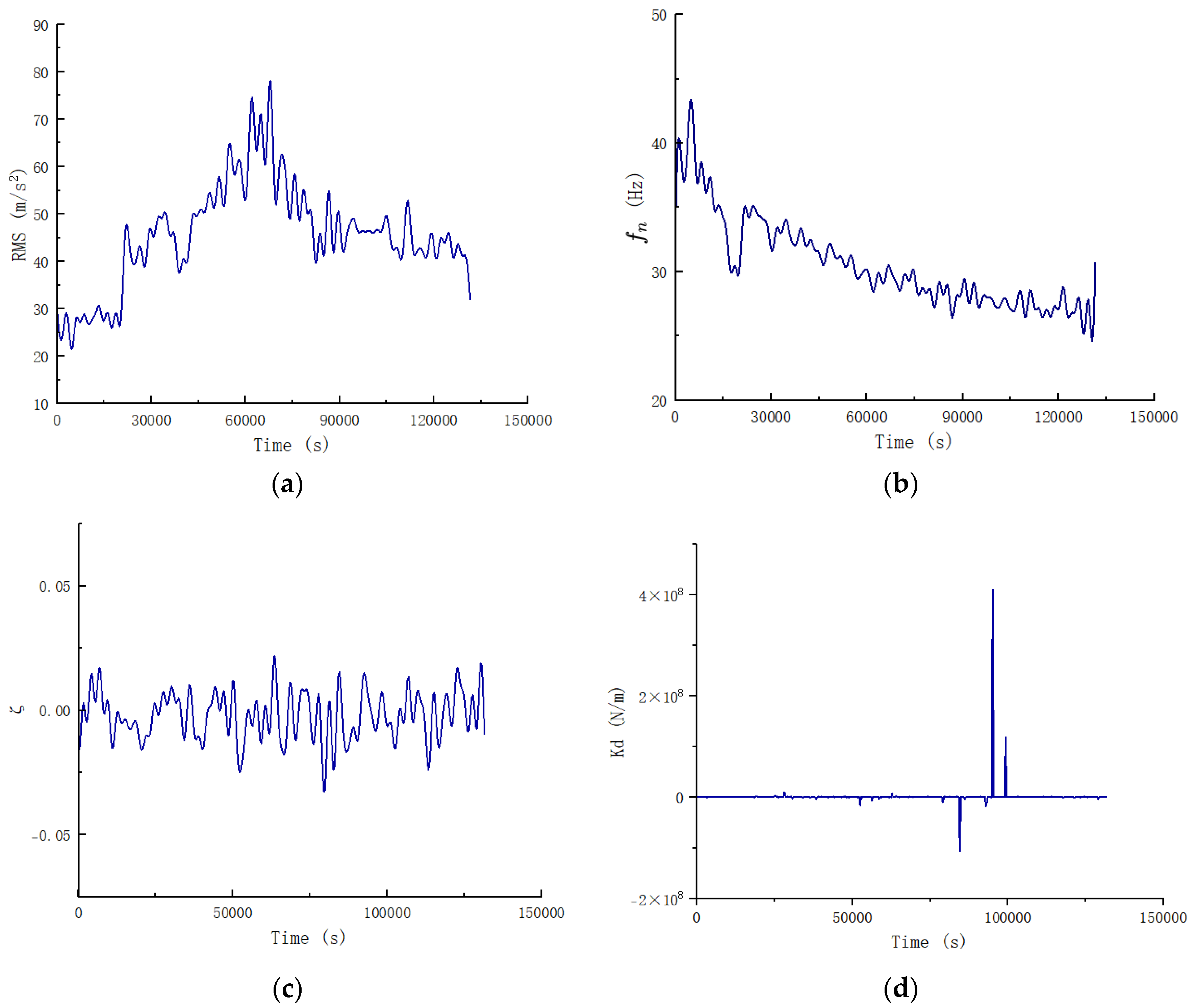
Based on the failure mechanism of elastic supports (stiffness attenuation and damping characteristic changes caused by material fatigue), four characteristic parameters with physical meaning were selected. The characteristic curves are shown in Figure 6. The definitions and physical meaning of these parameters are as follows:
1. Root Mean Square (RMS) acceleration: RMS reflects the energy level of vibration signals and is directly related to the vibration energy dissipation of support components (where a i is the acceleration value at the sampling point and N is the number of sampling points).
R M S = 1 N i = 1 N a i 2 a i ,
2. Natural frequency ( f n ): It is obtained by power spectrum analysis of the vibration signal. When the stiffness of the support decreases, the natural frequency decreases with increasing damage degree.
3. Damping ratio (ζ): The ζ is calculated using the half-power bandwidth method, reflecting the energy dissipation capability of the support member. The damping ratio increases significantly after damage (where the frequency corresponding to a 3 dB amplitude reduction in the power spectrum is taken as the reference).
ζ = f 2 f 1 2 f n ,
4. Stiffness ( K d ): Dynamic stiffness is calculated based on vibration signals and load signals, and its decay serves as a direct indicator of support failure (where F 0 is the load amplitude and A 0   is the vibration displacement amplitude).
K d = F 0 A 0 ,

3.2.4. Analysis and Selection of Characteristic Parameters

In this paper, a two-step progressive feature selection was adopted. Firstly, the Pearson correlation coefficient was used to identify the correlations among the original features, and redundant features weakly related to life were eliminated to complete the preliminary optimization. Then, the PCA principal component dimension reduction is carried out based on the effective original features retained by Pearson screening. Pearson acts on the original feature level, whereas PCA compresses the dimension of the optimized features. The division of labor is clear, and the feature logic confusion is avoided.
  • PCA screening
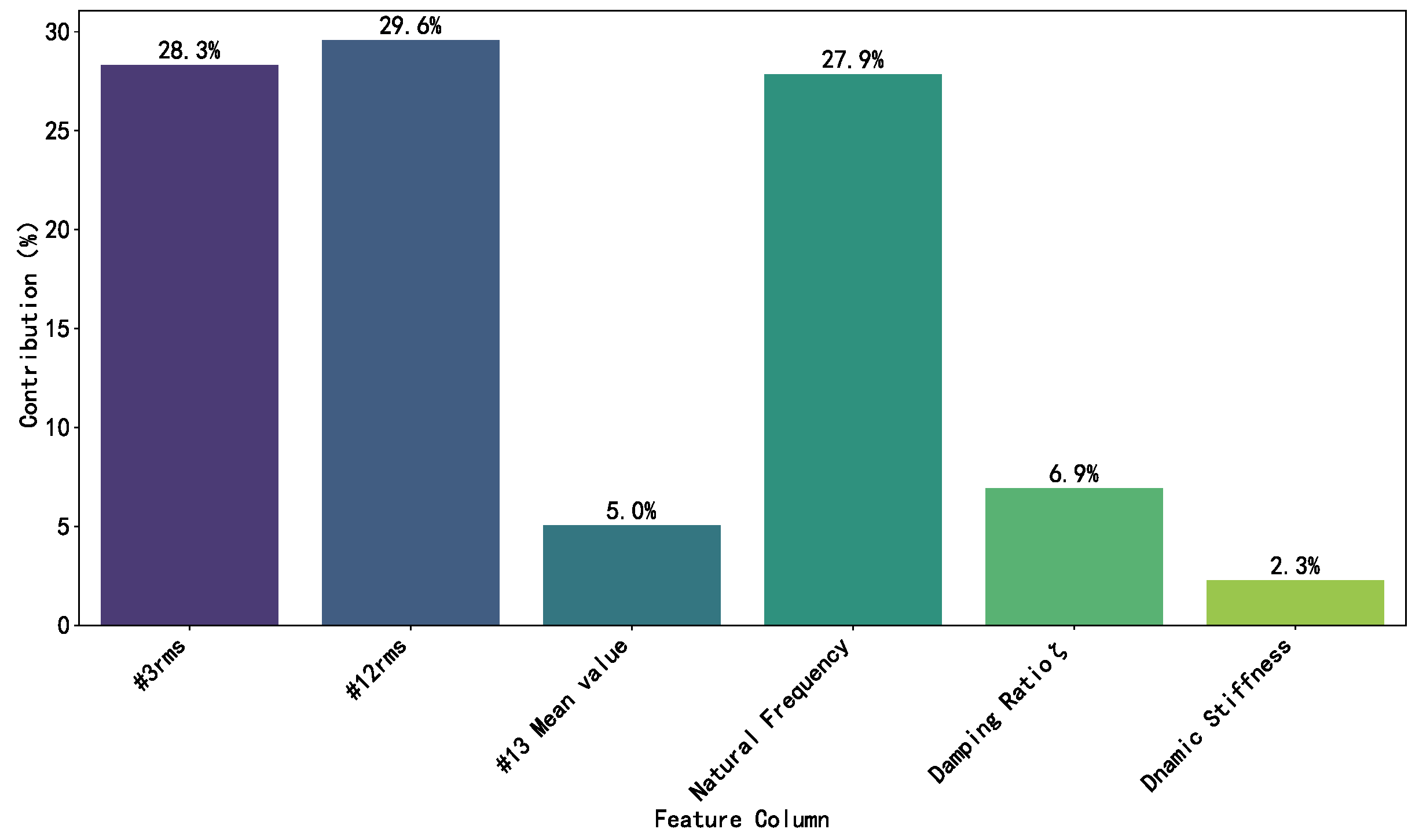
Figure 7 quantifies the loading coefficients of each original feature on the first principal component, which reflects the contribution degree of each feature to the core variation. The results show that the natural frequency f n (26.3%) and operating time (26.0%) have the highest contribution rates, followed by #12 RMS (20.7%) and #3 RMS (17.6%), which are the core features driving the degradation variation in elastic supports. The contribution rates of damping ratio (ζ) (5.0%), #13 mean value (2.8%), and dynamic stiffness K d (1.6%) are relatively low, indicating that these features contain less unique information and are highly redundant with other features.
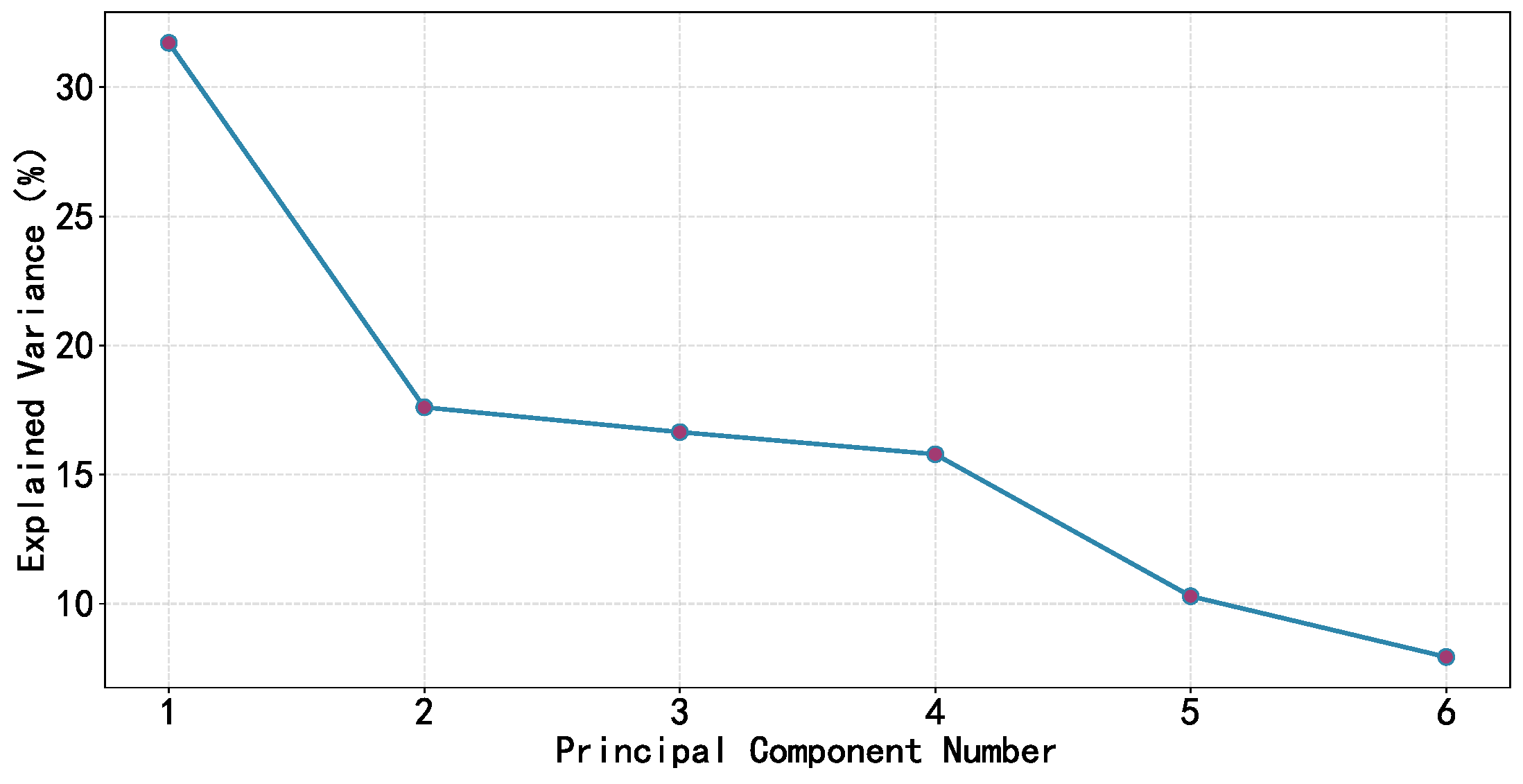
Figure 8 shows the variance explained rate of each principal component and the cumulative variance explained rate. The first principal component explains 35.2% of the total variance, the second principal component explains 28.7%, and the third principal component explains 28.4%. The cumulative variance explained rate of the first three principal components reaches 92.3%, which exceeds the preset threshold of 85%, indicating that the first three principal components can fully retain the core information of the original seven features. Therefore, the first three principal components were selected as the output of PCA screening, which not only reduced the feature dimensionality (from seven to three) but also eliminated multicollinearity.
2.
Pearson correlation analysis
To further verify the correlations between the original characteristic parameters and the service life of elastic supports, Pearson correlation analysis was performed between each original feature and the cyclic life. Here, the reciprocal of operating time was adopted as the life characterization index because operating time is negatively correlated with remaining life [35]. Table 2 lists the Pearson correlation coefficients between the key features and the life index. It can be seen that most feature parameters show high linear correlations with life, with absolute correlation coefficients generally above 0.85. In contrast, individual features present relatively weak correlations. Specifically: (1) the natural frequency f n has a strong negative correlation with life (r = −0.875), which is consistent with the failure mechanism; with the extension of service life, the support stiffness decreases and f n decreases; (2) #3 RMS has a strong positive correlation with life (r = 0.814), indicating that vibration energy dissipation increases with increasing service life; (3) #12 RMS has a moderate negative correlation with life (r = −0.217), which may be related to the sensor installation position (lower-flange vibration is less affected by support damage). These results confirm that the selected features are all damage-sensitive, and the natural frequency f_n is the most sensitive feature reflecting the damage evolution of the supports, which provides a reliable basis for subsequent model training.

3.3. Result Analysis and Discussion

3.3.1. Ablation Experiments

To verify the effectiveness of the optimization strategies (time decay factor and feature–parameter collaborative constraints) proposed in this study, ablation experiments were conducted with the traditional unoptimized random forest model as the benchmark. A total of 412 degradation samples were employed, with the training (288 samples) and test (124 samples) sets partitioned chronologically to avoid look-ahead bias associated with random sampling. To ensure rigorous comparative analysis, the experimental variables were strictly controlled: all models utilized identical feature sets and hyperparameter configurations, leaving the optimization strategy as the sole variable.
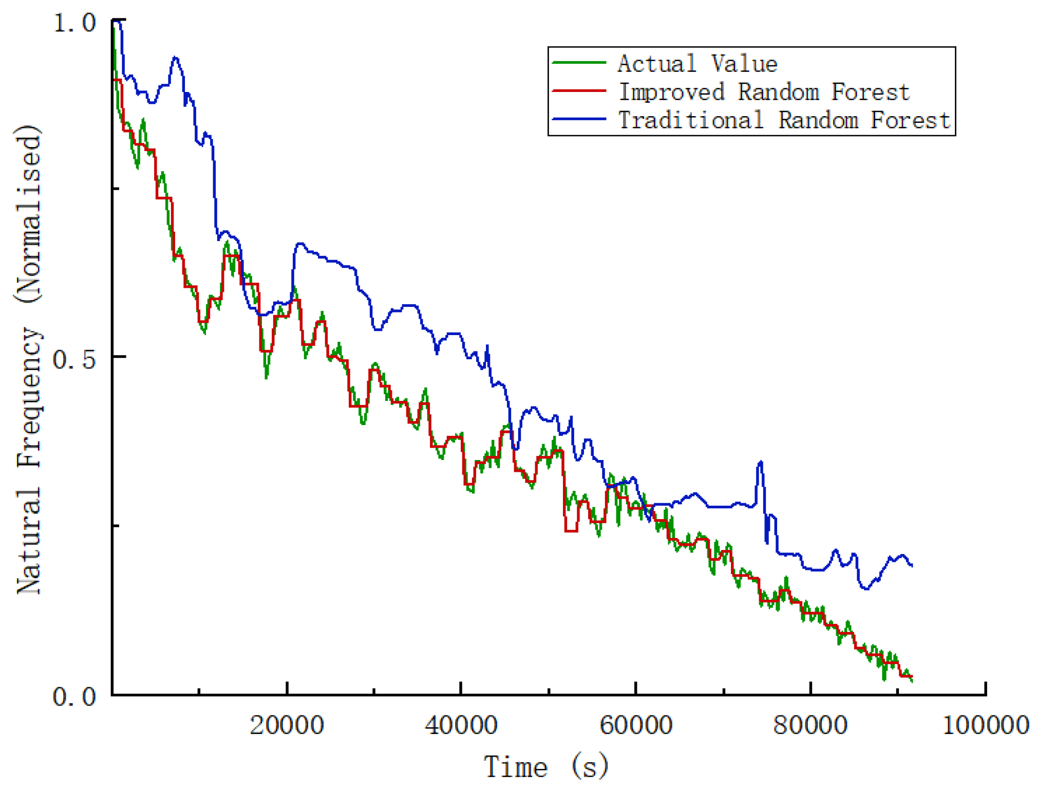
Figure 9 shows the comparison curves of the actual remaining life, the traditional random forest predictions, and the improved random forest predictions. It can be seen that: (1) In the early stage of service (0–40,000 s), the prediction curve of the improved random forest almost overlapped with the actual value curve, with a prediction error of less than 0.01, while the traditional random forest has a prediction deviation of 0.03–0.05, which is due to the time decay factor effectively capturing the initial slow degradation trend. (2) In the middle stage of service (40,000–100,000 s), the actual remaining life shows a nonlinear decay trend. The prediction fluctuations of the improved random forest are highly consistent with the actual values, while the traditional random forest exhibits obvious overestimation (predicted values higher than the actual values) in the interval of 60,000–80,000 s. (3) In the late stage of service (100,000–140,000 s), the degradation of the support accelerates. The improved random forest still maintains high prediction accuracy (error < 0.02), while the prediction error of the traditional random forest increases to 0.06–0.08. This visual comparison confirms that the improved random forest has superior fitting accuracy and nonlinear trend-capturing ability.
Table 3 lists the quantitative evaluation indicators of the two models on the test set. The improved random forest model achieved MSE = 0.007, RMSE = 0.026, and R2 = 0.988, which are significantly better than those of the traditional random forest (MSE = 0.115, RMSE = 0.055, and R2 = 0.915). Specifically: (1) RMSE is reduced by 52.7% (from 0.055 to 0.026), indicating that the average prediction error was nearly halved. (2) R2 increased by 7.9% (from 0.915 to 0.988), indicating that the model’s ability to explain data variation was significantly enhanced. The results of the comparative experiment fully verify that the introduction of the time decay factor and feature–parameter collaborative constraints effectively improves the model’s ability to capture temporal decay trends and resist overfitting, thereby significantly improving prediction accuracy and stability.

3.3.2. Comparative Experiments

To further verify the comprehensive performance of the proposed improved random forest model, comparative experiments were conducted with three mainstream life prediction algorithms as benchmarks: Gray Prediction (GM(1,1) model), BP Neural Network (three-layer structure: input layer with three neurons, hidden layer with ten neurons, and output layer with one neuron), and XGBoost (extreme gradient boosting tree). All models use the same training set (288 groups) and test set (124 groups), while the input features are the three principal components screened by PCA to ensure a fair comparison. The hyperparameters of the benchmark models are optimized using the same Randomized Search CV method: (1) Gray Prediction: background value coefficient is set to 0.4; (2) BP Neural Network: learning rate = 0.01, training epochs = 1000, and batch size = 32; and (3) XGBoost: n e s t i m a t o r s = 100, m a x d e p t h = 10, and m i n s a m p l e s   s p l i t = 5.
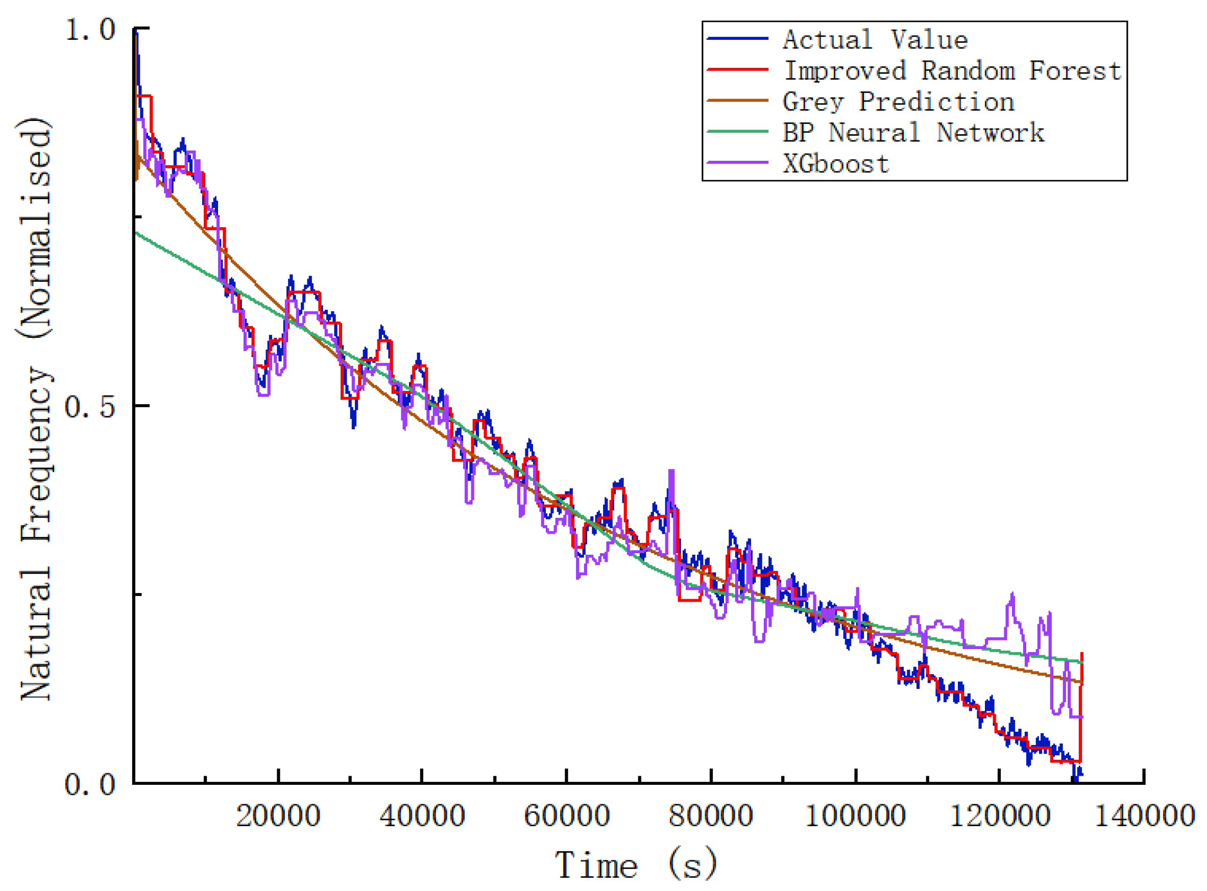
Figure 10 shows the comparison curves of the actual remaining life and the predicted values of the four models. It can be seen that: (1) The prediction curve of the improved random forest is closest to the actual value curve in both the overall trend and local fluctuations, and its fitting effect is significantly better than those of the other three models. (2) Gray Prediction has a large deviation in the early stage (0–40,000 s) (predicted values are much lower than the actual values), which is due to its poor adaptability to nonlinear degradation data. (3) The BP Neural Network exhibits overfitting in the middle stage (40,000–80,000 s), and the prediction trend is significantly inconsistent with the actual value. (4) XGBoost has a good fitting effect in the middle stage but underestimates the remaining life in the late stage (100,000–140,000 s) (predicted values are lower than the actual values), which is due to its sensitivity to extreme values in small-sample scenarios. This intuitive comparison shows that the improved random forest has stronger nonlinear trend-capturing ability and robustness.
In order to systematically and quantitatively assess the performance differences in different prediction models, we systematically present the specific values of four algorithms in Table 4. These algorithms include the improved random forest, Gray Prediction, BP Neural Network and XGBoost. The values correspond to their performance on the three core evaluation metrics.
In terms of MSE, the improved random forest and XGBoost significantly outperformed the BP Neural Network and Gray Prediction models, demonstrating a superior capability to mitigate cumulative squared errors. As RMSE further characterizes the magnitude of prediction bias, the improved random forest achieved the lowest value (0.026), indicating the highest precision and the smallest dispersion among individual sample predictions. Furthermore, regarding the goodness-of-fit measured by R2, the improved random forest reached 0.988, suggesting that 98.8% of the data variance was captured by the model, thereby confirming a robust linear correlation between the predicted and actual values. In contrast, the BP and Gray Prediction models exhibited lower R2 scores, highlighting their limited capacity to capture the underlying degradation patterns.
Although XGBoost yielded a marginally lower MSE, the improved random forest demonstrated a more robust and comprehensive performance profile. The evaluation across multiple dimensions, including error minimization, goodness-of-fit, and stability in tracking degradation trends, indicates that the improved random forest provides a more balanced and reliable prediction. This suggests that relying on a single metric may be insufficient for model assessment. When considered holistically, the proposed improved random forest exhibits superior generalization and the most effective overall prediction performance.
To improve the interpretability of the proposed model and alleviate the “black-box” drawback of tree-based ensemble methods, SHAP (SHapley Additive exPlanations) analysis is adopted in this study [36]. According to the Pearson correlation and PCA feature contribution results, natural frequency and acceleration RMS are recognized as the most critical features for RUL prediction, whose variation rules accord well with the physical degradation mechanism of stiffness attenuation and fatigue-induced vibration enhancement of elastic supports. Meanwhile, the introduced time decay factor further enables the model to capture the time-dependent degradation trend in the full-life stage. Therefore, the superior prediction performance of the improved random forest is attributed to its effective learning of physically meaningful degradation features and temporal evolution regularity, instead of pure data fitting. The SHAP analysis establishes a quantitative relationship between model outputs and damage evolution, which greatly enhances the interpretability and engineering reliability of the data-driven prediction model.

4. Conclusions

This study addressed the remaining life prediction of elastic supports and established a technical framework of “signal acquisition–feature extraction–feature screening–life prediction”, achieving accurate life prediction via experimental verification and algorithm optimization. Key conclusions are as follows:
  • Vibration signal features (acceleration RMS, natural frequency, etc.) can effectively characterize the damage state of elastic supports. Natural frequency is the core sensitive feature, exhibiting an absolute correlation coefficient of 0.875 with the life characterization index.
  • The combined feature screening strategy of PCA and Pearson correlation coefficient performs well by reducing dimensions, eliminating redundancy, enhancing feature-life correlation, and improving the efficiency and accuracy of subsequent model training.
  • The optimized random forest model with a time decay factor and feature–parameter synergistic constraints exhibits excellent performance, effectively alleviating overfitting and the dimensional disaster of small-sample data. The model’s RMSE is 0.026 and R2 reaches 0.988, significantly outperforming the Gray Prediction, BP Neural Network and XGBoost algorithms.
  • The proposed approach features good engineering applicability, enabling online real-time life prediction without offline disassembly and providing an efficient solution for predictive maintenance of elastic supports. Future research will expand sample sizes, enrich feature systems with nonlinear extraction methods and explore fusion with deep learning models to improve prediction performance under extreme working conditions.
While this study successfully captures the degradation patterns of elastic supports via accelerated life-cycle testing, the framework faces two primary limitations. First, restricted by the high costs of components and the prolonged duration of full-life tests, the dataset was confined to 412 samples from a single specimen, which may constrain model generalization. Second, laboratory conditions do not fully encapsulate the complexities of actual operations, such as variable loads, thermal fluctuations, and signal interference. Future work will address these limitations by expanding the experimental scale and integrating data under complex conditions.

Author Contributions

Conceptualization, W.Z. and J.H.; Methodological Work, W.Z.; Validation Work, Z.F., Y.D., W.W. and J.W.; Data Organization Work, W.Z.; Original Draft Writing, W.Z.; Review and Editing Work, Z.F. and W.Z.; Visualization Work, W.Z.; Project Management, J.H.; Funding Acquisition Work, J.H. All authors have read and agreed to the published version of the manuscript.

Funding

This research received no external funding.

Data Availability Statement

The data are not publicly available due to privacy or ethical restrictions.

Conflicts of Interest

The authors declare no conflicts of interest.

References

  1. Liu, X.-A.; Zhang, J.; Jia, X.; Xiao, S.; Chen, D.; Shangguan, W.-B. Modeling and analysis of dynamic characteristics of rubber isolators for electric vehicles under high-frequency excitation. Proc. Inst. Mech. Eng. Part D J. Automob. Eng. 2023, 237, 2942–2956. [Google Scholar] [CrossRef] [Scilit]
  2. Zhang, B.; Zhao, Y.; You, J.; Zhang, Z. Experimental and numerical analysis of rubber isolator dynamic stiffness under hydrostatic pressure. Ocean. Eng. 2024, 314, 119650. [Google Scholar] [CrossRef] [Scilit]
  3. Zhang, Y.; Fu, W.; Wang, L. Modeling analysis of a novel hybrid 6-DOF vibration isolation platform for sensitive instruments. In Journal of Physics: Conference Series, Proceedings of the 2022 8th International Conference on Mechanical Engineering, Materials and Automation Technology (MMEAT 2022), Qingdao, China, 27–29 May 2022; IOP Publishing: Bristol, UK, 2022. [Google Scholar] [CrossRef] [Scilit]
  4. Xiao, C.; Wang, H.; Li, Z.; Zhang, J.; Han, Y.; Fang, L.; Qu, Z.; Liu, J.; Du, M. Failure analysis and life prediction of electronic devices in aerospace engines under random vibration. Measurement 2025, 256, 118282. [Google Scholar] [CrossRef] [Scilit]
  5. Long, X.-H.; Ma, Y.-T.; Yue, R.; Fan, J. Experimental study on impact behaviors of rubber shock absorbers. Constr. Build. Mater. 2018, 173, 718–729. [Google Scholar] [CrossRef] [Scilit]
  6. Apsemetov, M.; Madanbekov, N.; Muktarov, T. Determination of the own forms of vibration of the span of beam bridges on elastic supporting parts. In E3S Web of Conferences, Proceedings of the XXIV International Scientific Conference “Construction the Formation of Living Environment” (FORM-2021), Moscow, Russia, 22–24 April 2021; EDP Sciences: Paris, France, 2021. [Google Scholar] [CrossRef] [Scilit]
  7. Shangguan, W.B.; Liu, T.K.; Wang, X.L.; Xu, C.; Yu, B. A method for modelling of fatigue life for rubbers and rubber isolators. Fatigue Fract. Eng. Mater. Struct. 2014, 37, 623–636. [Google Scholar] [CrossRef] [Scilit]
  8. Pöschl, M.; Vašina, M.; Zádrapa, P.; Měřínská, D.; Žaludek, M. Study of carbon black types in SBR rubber: Mechanical and vibration damping properties. Materials 2020, 13, 2394. [Google Scholar] [CrossRef] [Scilit]
  9. Zheng, Z.; Shi, L.; Cui, L. Multi-Data Fusion-Based Bearing Load Prediction Model for Elastically Supported Shafting Systems. Appl. Sci. 2026, 16, 733. [Google Scholar] [CrossRef] [Scilit]
  10. Ma, H.; Zhu, S.-P.; Guo, Y.; Pan, L.; Yang, S.; Meng, D. Residual useful life prediction of the vehicle isolator based on Bayesian inference. Structures 2023, 58, 105518. [Google Scholar] [CrossRef] [Scilit]
  11. Beijen, M.A.; Heertjes, M.F.; Butler, H.; Steinbuch, M. Disturbance feedforward control for active vibration isolation systems with internal isolator dynamics. J. Sound. Vib. 2018, 436, 220–235. [Google Scholar] [CrossRef] [Scilit]
  12. Sun, Y.-P.; Feng, H.; Zheng, B.; Wen, J.-R.; Chao, A.-F.; Fei, C.-W. Multi-Agent Reinforcement Symbolic Regression for the Fatigue Life Prediction of Aircraft Landing Gear. Aerospace 2025, 12, 718. [Google Scholar] [CrossRef] [Scilit]
  13. Smalakys, L.; Melninkaitis, A. Predicting lifetime of optical components with Bayesian inference. Opt. Express 2021, 29, 903–915. [Google Scholar] [CrossRef] [Scilit] [PubMed]
  14. Sun, S.; Wen, Z.; Zhang, W.; Wang, J.; Gao, H. On-line mechanical life prediction method for a conventional circuit breaker based on multi-parameter particle swarm optimization-support vector regression using vibration detection. Meas. Sci. Technol. 2022, 33, 095110. [Google Scholar] [CrossRef] [Scilit]
  15. Apicella, G.; Sibillo, M. Corrective factors for longevity projections in a dynamic context. Eur. Actuar. J. 2018, 8, 53–68. [Google Scholar] [CrossRef] [Scilit]
  16. Wang, J.; Wang, X.; Wang, L. Modeling of BN lifetime prediction of a system based on integrated multi-level information. Sensors 2017, 17, 2123. [Google Scholar] [CrossRef] [Scilit]
  17. Wang, Z.-Q.; Hu, C.-H.; Fan, H.-D. Real-time remaining useful life prediction for a nonlinear degrading system in service: Application to bearing data. IEEE/ASME Trans. Mechatron. 2017, 23, 211–222. [Google Scholar] [CrossRef] [Scilit]
  18. Kim, M.; Cheng, J.-R.C.; Liu, K. An adaptive sensor selection framework for multisensor prognostics. J. Qual. Technol. 2021, 53, 566–585. [Google Scholar] [CrossRef] [Scilit]
  19. Li, N.; Gebraeel, N.; Lei, Y.; Fang, X.; Cai, X.; Yan, T. Remaining useful life prediction based on a multi-sensor data fusion model. Reliab. Eng. Syst. Saf. 2021, 208, 107249. [Google Scholar] [CrossRef] [Scilit]
  20. Zhang, Y.; Shu, T.; Ding, R. Bearing Life Prediction Based on SPSS and Grey Prediction Model. In IOP Conference Series: Earth and Environmental Science, Proceedings of the 2020 2nd International Conference on Civil Engineering, Environment Resources and Energy Materials, Changsha, China, 18–20 September 2020; IOP Publishing: Bristol, UK, 2021. [Google Scholar] [CrossRef] [Scilit]
  21. Li, X.; Yang, X.; Yang, Y.; Bennett, I.; Mba, D. A novel diagnostic and prognostic framework for incipient fault detection and remaining service life prediction with application to industrial rotating machines. Appl. Soft Comput. 2019, 82, 105564. [Google Scholar] [CrossRef] [Scilit]
  22. Niu, Q.; Tong, Q.; Cao, J.; Zhang, Y.; Liu, F. On-line prediction remaining useful life for ball bearings via grey NARX. J. Vibroeng. 2019, 21, 82–96. [Google Scholar] [CrossRef] [Scilit]
  23. Wang, Y.; Zhang, H.; Xu, H.; Liu, J.; Guo, Y. Research on the gear bending fatigue full-life prediction model of considering hobbing residual stress. Precis. Eng. 2025, 95, 551–565. [Google Scholar] [CrossRef] [Scilit]
  24. Xu, L.; Xiong, L.; Zhang, R.; Zheng, J.; Zou, H.; Li, Z.; Wang, X.; Wang, Q. Data-Enhanced Low-Cycle Fatigue Life Prediction Model Based on Nickel-Based Superalloys. Acta Mech. Solida Sin. 2025, 38, 612–623. [Google Scholar] [CrossRef] [Scilit]
  25. Wu, Z.; Wang, Z.; Wei, H.; Ren, J.; Yuan, Y.; Wang, T.; Duan, W.; Wei, H.; Wang, S. Remaining useful life prediction for equipment based on RF-BiLSTM. AIP Adv. 2022, 12, 115209. [Google Scholar] [CrossRef] [Scilit]
  26. Liu, Q.; Shi, W.; Chen, Z. Rubber fatigue life prediction using a random forest method and nonlinear cumulative fatigue damage model. J. Appl. Polym. Sci. 2020, 137, 48519. [Google Scholar] [CrossRef] [Scilit]
  27. Wang, X.; Shangguan, W.; Rakheja, S.; Li, W.; Yu, B. A method to develop a unified fatigue life prediction model for filled natural rubbers under uniaxial loads. Fatigue Fract. Eng. Mater. Struct. 2014, 37, 50–61. [Google Scholar] [CrossRef] [Scilit]
  28. Liu, Y.; Song, J.; Zhao, Z.; Ye, G.; Liu, Z.; Zhou, Y. Adaptive residual life prediction for small samples of mechanical products based on feature matching preprocessor-LSTM. Appl. Sci. 2022, 12, 8236. [Google Scholar] [CrossRef] [Scilit]
  29. Duan, C.; Shen, Y.; Guo, K.; Sheng, B.; Wang, Y. Remaining useful life prediction based on a PCA and similarity methods. Meas. Sci. Technol. 2023, 35, 035020. [Google Scholar] [CrossRef] [Scilit]
  30. Zhang, B.; Wang, H.; Tang, Y.; Pang, B.; Gao, X. Residual useful life prediction for slewing bearing based on similarity under different working conditions. Exp. Tech. 2018, 42, 279–289. [Google Scholar] [CrossRef] [Scilit]
  31. Mantas, C.J.; Castellano, J.G.; Moral-García, S.; Abellán, J. A comparison of random forest based algorithms: Random credal random forest versus oblique random forest. Soft Comput. 2019, 23, 10739–10754. Available online: https://www.x-mol.com/paperRedirect/1335456250456404001. [CrossRef] [Scilit]
  32. Breiman, L. Random forests. Mach. Learn. 2001, 45, 5–32. [Google Scholar] [CrossRef] [Scilit]
  33. Sun, Z.; Wang, G.; Li, P.; Wang, H.; Zhang, M.; Liang, X. An improved random forest based on the classification accuracy and correlation measurement of decision trees. Expert Syst. Appl. 2024, 237, 121549. [Google Scholar] [CrossRef] [Scilit]
  34. Li, C.; Sánchez, R.V.; Zurita, G.; Cerrada, M.; Cabrera, D.; Vásquez, R.E. Gearbox fault diagnosis based on deep random forest fusion of acoustic and vibratory signals. Mech. Syst. Signal Process. 2016, 76, 283–293. [Google Scholar] [CrossRef] [Scilit]
  35. Wang, Y.; Zhao, J.; Yang, C.; Xu, D.; Ge, J. Remaining useful life prediction of rolling bearings based on Pearson correlation-KPCA multi-feature fusion. Measurement 2022, 201, 111572. [Google Scholar] [CrossRef] [Scilit]
  36. Bernal, L.; Rastelli, G.; Pinzi, L. Improving machine learning classification predictions through SHAP and features analysis interpretation. J. Chem. Inf. Model. 2025, 65, 11716–11732. [Google Scholar] [CrossRef] [Scilit] [PubMed]
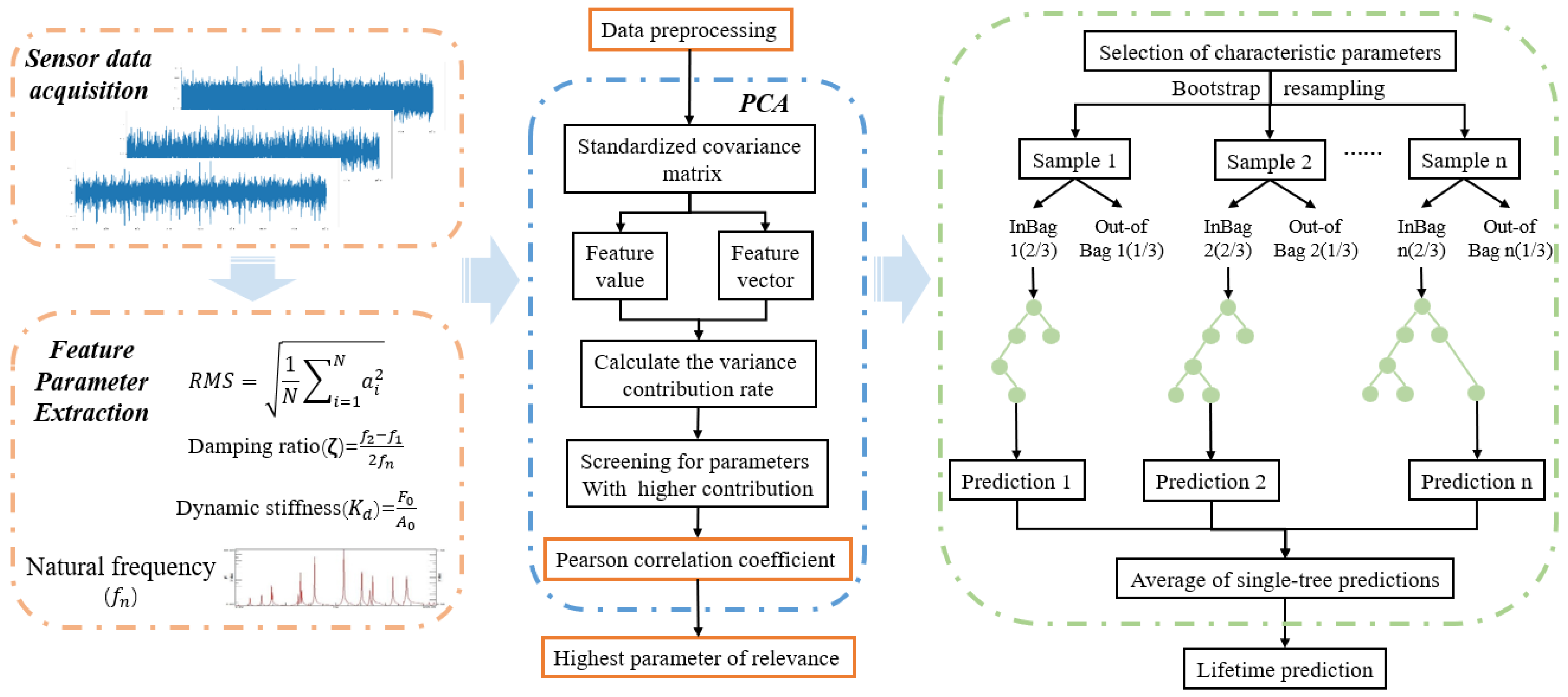
Figure 1. Overall framework diagram of the experiment.
Machines 14 00547 g001
Figure 2. Improving the framework of the random forest algorithm.
Machines 14 00547 g002
Figure 3. Overall experimental procedure.
Machines 14 00547 g003
Figure 4. Schematic diagram of a vibration table with elastic supports throughout its entire service life.
Machines 14 00547 g004
Figure 5. Schematic diagram of a vibration table with elastic supports throughout its entire service life. (a) Initial state of the elastic support component; (b) Sample No. 2025030001; (c) Sample No. 2025030003; and (d) Sample No. 2025030006.
Machines 14 00547 g005
Figure 6. Schematic diagram of a vibration table with elastic supports throughout its entire service life. (a) Effective value curve of acceleration; (b) effective value of natural frequency; (c) damping ratio curve; and (d) dynamic stiffness curve.
Machines 14 00547 g006
Figure 7. Column chart showing the contribution of each column to the first principal component.
Machines 14 00547 g007
Figure 8. Line graph of variance explained by each principal component.
Machines 14 00547 g008
Figure 9. Comparison of prediction results between the improved random forest and the traditional random forest.
Machines 14 00547 g009
Figure 10. Comparison of prediction results among multiple algorithms.
Machines 14 00547 g010
Table 1. Hyperparameters.
HyperparameterNumeric Value
n e s t i m a t o r s 100
m a x d e p t h 10
m i n s a m p l e s   s p l i t 5
random seed42
number of iterations of random search12
cross-validation fold3
Table 2. Pearson correlation coefficient.
Characteristic Parameter#3RMS#12RMS f n
Correlation0.814−0.217−0.875
Table 3. Compare experimental evaluation metrics of the baseline algorithms.
MethodMSERMSER2
Traditional random forest0.1150.0550.915
Improved random forest0.0070.0260.988
Table 4. Comparison of experimental evaluation indicators.
MethodMSERMSER2
Improved random forest0.0070.0260.988
Gray Prediction0.0070.0860.832
BP Neural Network0.0060.0800.862
XGBoost0.0050.0600.923
Disclaimer/Publisher’s Note: The statements, opinions and data contained in all publications are solely those of the individual author(s) and contributor(s) and not of MDPI and/or the editor(s). MDPI and/or the editor(s) disclaim responsibility for any injury to people or property resulting from any ideas, methods, instructions or products referred to in the content.