Transient Coupled Dynamics Analysis of a High-Pressure Plunger Pump with Electrical–Mechanical–Hydraulic Interaction

Abstract

Plunger pumps are widely used in high-pressure and high-flow applications and exhibit strong adaptability to different fluid media. In addition to the interaction between the valve and the fluid, a potential coupling effect may exist between the flow characteristics of the pump and the electromagnetic characteristics of the motor. To investigate the electromagnetic–mechanical–hydraulic coupling effect in a motor–pump system, a transient coupled dynamics model integrating electromagnetic fields (EMF), multi-body dynamics (MBD), and computational fluid dynamics (CFD) is developed. The motion of the valve is incorporated into the model through dynamic mesh and user-defined function (UDF) techniques. The different physical models are coupled through torque, speed, force, and displacement. Based on the proposed model, the coupling characteristics of the system are analyzed. The results show that pulsating components associated with the reciprocating frequency appear in both the rotational speed and torque of the motor, resulting in fluctuations of approximately 2.11% in speed and 29.57% in torque. These pulsations are also reflected in the stator current spectrum. In addition, the valve motion at different crank angles and the flow patterns in the pump chamber are analyzed. The electromagnetic characteristics of the motor have a limited influence on the internal flow behavior of the pump.

1. Introduction

The plunger pump is a type of reciprocating pump that is widely used in the petroleum and chemical industries to satisfy the requirements for high pressure and high flow rates [1]. The rotational motion of the crankshaft is converted into the reciprocating motion of the plungers, which causes the working medium to be alternately sucked into and discharged from the chambers. Valves are installed in each chamber and are designed to close automatically under the action of spring force or gravity and to open when the hydraulic force exceeds the spring or gravitational force. This self-actuating mechanism ensures that the fluid flows only from the inlet to the outlet.

The fluid–structure interaction (FSI) has attracted considerable attention. The interaction between the fluid and structural parts has varying effects depending on the part type. On the one hand, the interaction with movable parts, such as valves and plungers, changes their state of motion [2]. On the other hand, the interaction with fixed components, such as cylinders, induces elastic deformation, which in turn generates vibration and noise [3].

Recent research on FSI of plunger pumps has mainly focused on valve dynamics and flow characteristics. Aakre et al. demonstrated the correlation between valve dynamics and pump volumetric efficiency [4]. Owing to the spring preload and valve lift, the valve opening and closing typically exhibit a phase lag [5]. Ma et al. investigated the effects of valve parameters, including spring stiffness, preload, and lift, on this phase lag [6]. A smaller spring force decreases the opening lag but increases the closing lag. In contrast, a larger spring force reduces the closing lag of the valve but increases the opening lag, consequently leading to more severe impacts between the valve plate and the valve seat. To balance the impact and the lag, Zhu et al. proposed a variable-stiffness valve structure [7]. Moreover, the rotational speed and outlet pressure also affect the valve dynamics [8]. Zhao et al. developed an FSI model for a high-pressure plunger pump to simulate the flow characteristics in the clearance between the plunger and the plunger sleeve [9]. Dong et al. established a CFD model for a high-pressure reciprocating pump to investigate the relationship between the suction coefficient and valve motion, the mechanism of turbulence generation, and the two-stage throttling phenomenon occurring during the lifting process of the suction valve disk [10].

The models considering FSI can mainly be classified into three types: (i) lumped-parameter models, (ii) spatially discretized models, and (iii) hybrid models. Qiu et al. developed a lumped-parameter model for reciprocating liquid hydrogen pumps by integrating the plunger and valve motion equations with the fluid continuity, energy balance, and efficiency equations [11]. This type of model is well known for its simplicity and low computational cost. Based on the finite volume method, Munsch et al. established a numerical discretization model to study the effect of reflected pressure waves or expansion waves from the inlet boundary on partial cavitation [12]. The main advantage of spatially discretized models lies in their ability to describe complex flow phenomena, such as cavitation and water-hammer effects, but their high computational cost limits their widespread application. Hybrid models combine the advantages of the two approaches and achieve a balance between computational efficiency and accuracy. In such models, spatially discretized models are employed in the domain of interest, while lumped-parameter models are used in other regions. For example, Munsch et al. developed a 3D/1D seamlessly coupled model in which the pump domain where cavitation occurs was simulated using three-dimensional (3D) computational fluid dynamics (CFD), whereas the pipelines were modeled using the one-dimensional method of characteristics [13].

The studies mentioned above provide a thorough understanding of FSI in reciprocating pumps. However, the coupling interactions between the driving motor and the pump have rarely been considered. Owing to advantages in system efficiency, vibration and noise performance, and controllability, electrical machines are commonly used to drive plunger pumps [14]. The pump and the motor are connected through a reduction drive to convert electrical energy into hydraulic energy. Numerous studies have demonstrated that coupling effects are common between electrical machines and their loads.

Szolc et al. investigated the coupling effects between a rotating machinery and its drive motor system, calculated the electromagnetic stiffness and damping introduced by the motor, and studied the influence of electrical parameters on mechanical transmission [15]. Chen et al. studied the electrical–mechanical and rigid–flexible coupling effects among the gear transmission system, generator system, and control system in wind power generation and found that the vibration and dynamic meshing force of the gear system were affected by electromagnetic excitation, while the vibration and output current of the generator were also influenced by internal excitation from the gear system [16]. Mauri et al. analyzed the torsional vibration of the shaft system in a dual-inertia system including an electric motor. They also investigated potential vibration behavior caused by the overlap between pulsating torque harmonics introduced by the motor and its control system and the natural frequencies of the shaft system [17]. Liu et al. calculated the dynamic response of an electric vehicle powertrain and demonstrated that electromagnetic effects and the PI controller parameters of the control system can introduce new rotational modes and change the low-order natural frequencies of the system [18]. Shu et al. investigated the dynamic characteristics of a multi-motor drive system for a coal-cutting drum under three typical working conditions and showed that the stator current is affected by the mechanical characteristics of the transmission system [19].

Most studies on the coupling effects between pumps and motors focus on centrifugal pump systems. Zhao et al. proposed a multi-physics finite element simulation approach for a centrifugal pump system driven by a motor. By constructing the fluid load torque equation of the pump, the transient electromagnetic vibration of the motor was simulated and analyzed [20]. Nan et al. investigated the vibration of a centrifugal pump under fluid and motor excitations. In their study, the fluid and motor excitations were obtained from CFD simulations and experiments, respectively [21]. For centrifugal pump systems, Dong et al. developed a multi-field coupling simulation model that includes the motor, shaft, and pump, based on the finite element, modal superposition, and finite volume methods. The results indicate that the operating conditions of the pump are influenced by the rotating shaft and the driving motor [22]. In contrast to centrifugal pumps, plunger pumps have a distinct working mechanism and exhibit a more complex operating process. Therefore, it is necessary to investigate the interaction between plunger pumps and motors.

To account for the complex interactions within the plunger pump system, a system-level simulation model is required to describe its dynamic behavior. Therefore, a novel transient coupled dynamic model considering the electromagnetic–mechanical–hydraulic coupling effects is proposed. In this model, the finite element method is used to compute the electromagnetic characteristics of the induction motor, multi-body dynamics (MBD) is employed to describe the motion of the crankshaft mechanism, and CFD is applied to capture the internal flow characteristics of the pump. The different physical models are coupled by exchanging coupling variables. The electrical characteristics of the induction motor, the valve dynamics, and the internal flow characteristics of the pump are calculated, and the interaction between the pump and the motor is discussed.

The contributions of this study are summarized as follows: (a) A comprehensive coupled modeling framework is developed to account for the interactions among the motor, fluid, and valve–plunger dynamics. This modeling framework is applicable to problems involving three or more physical domains. (b) The coupling mechanism between the motor and the plunger pump is clarified. Due to the modulation effect, the periodic load of the pump induces sideband harmonics in the motor speed, torque, and current spectra. The speed ripple generated by the motor has a limited influence on pump performance, providing new insights into the motor–pump coupling mechanism. (c) The influence of compressibility in valve dynamics and flow rate pulsation is revealed. The delay in valve opening is the main cause of pump flow pulsation, and the compressibility of the fluid significantly increases the valve opening delay.

2. Geometry Structure and Fundamental Parameters

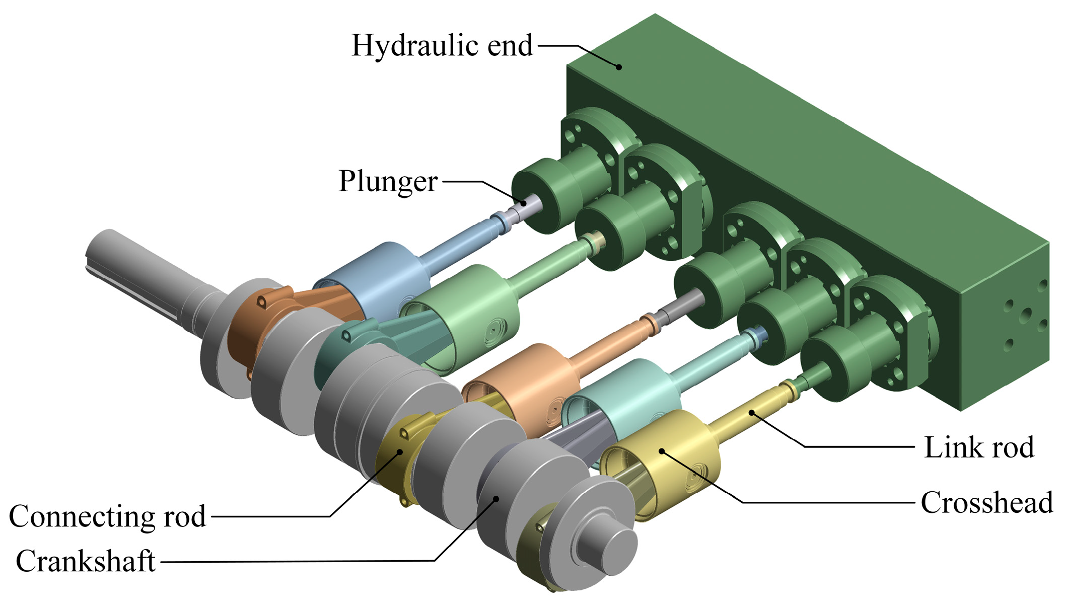
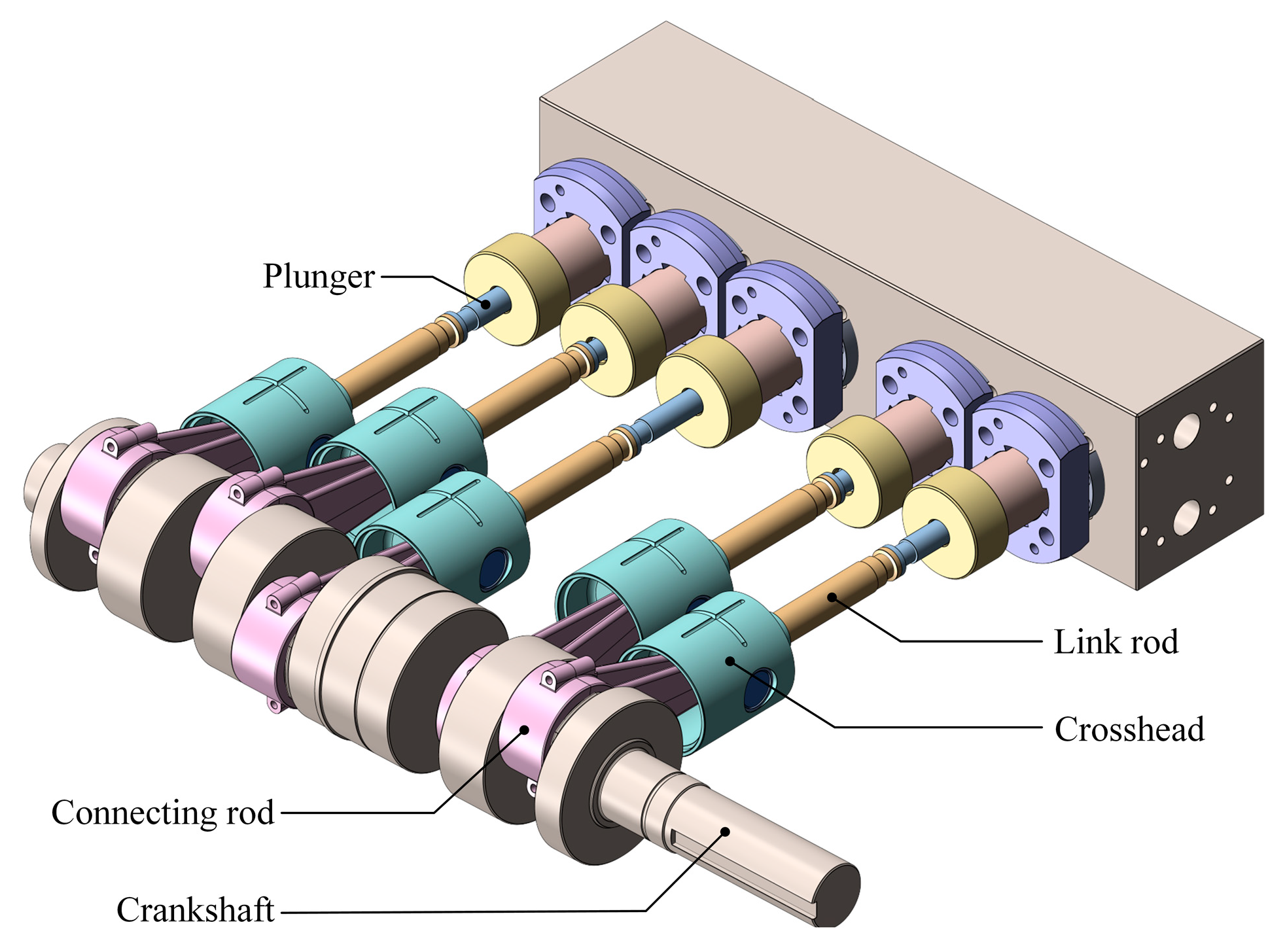
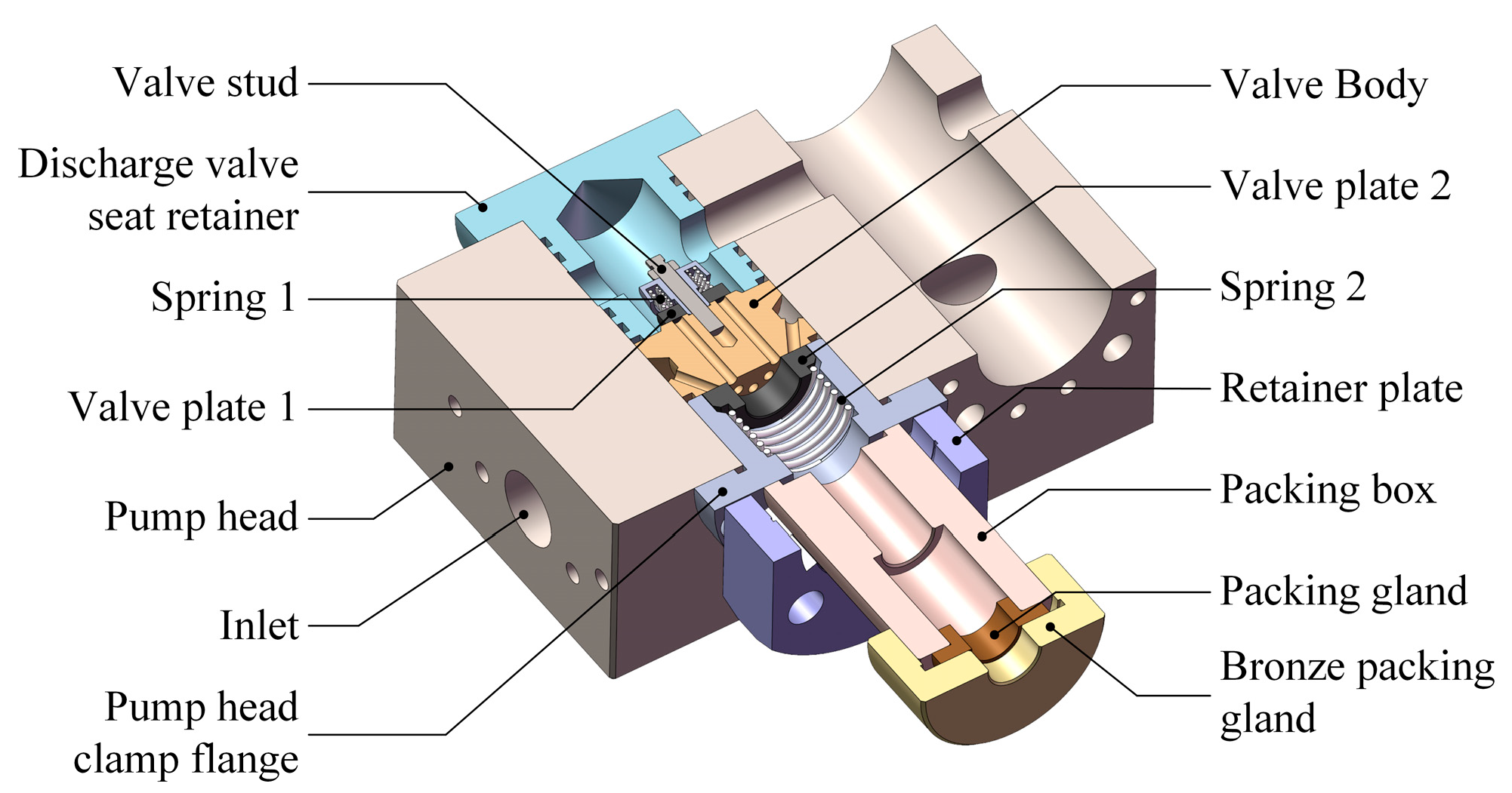
A high-pressure five-cylinder plunger pump used for water transport in the petroleum industry is investigated in this study. The geometric structure of the pump is shown in Figure 1. To reduce flow and pressure pulsations, the pump adopts a five-cylinder parallel configuration. Figure 2 further illustrates the internal structure of the pump head. Specifically, a suction valve and a discharge valve, both equipped with spring mechanisms, are installed in each cylinder. The pump head is designed with two inlets and one outlet. The main parameters of the pump are listed in

Table 1. Main parameters of the plunger pump.

Parameter	Value	Unit
Rated pressure	37	MPa
Theoretical flow rate	15.9	m3/h
Reciprocating stroke	127	mm
Plunger diameter	38	mm
Reciprocating frequency	370	min−1

.

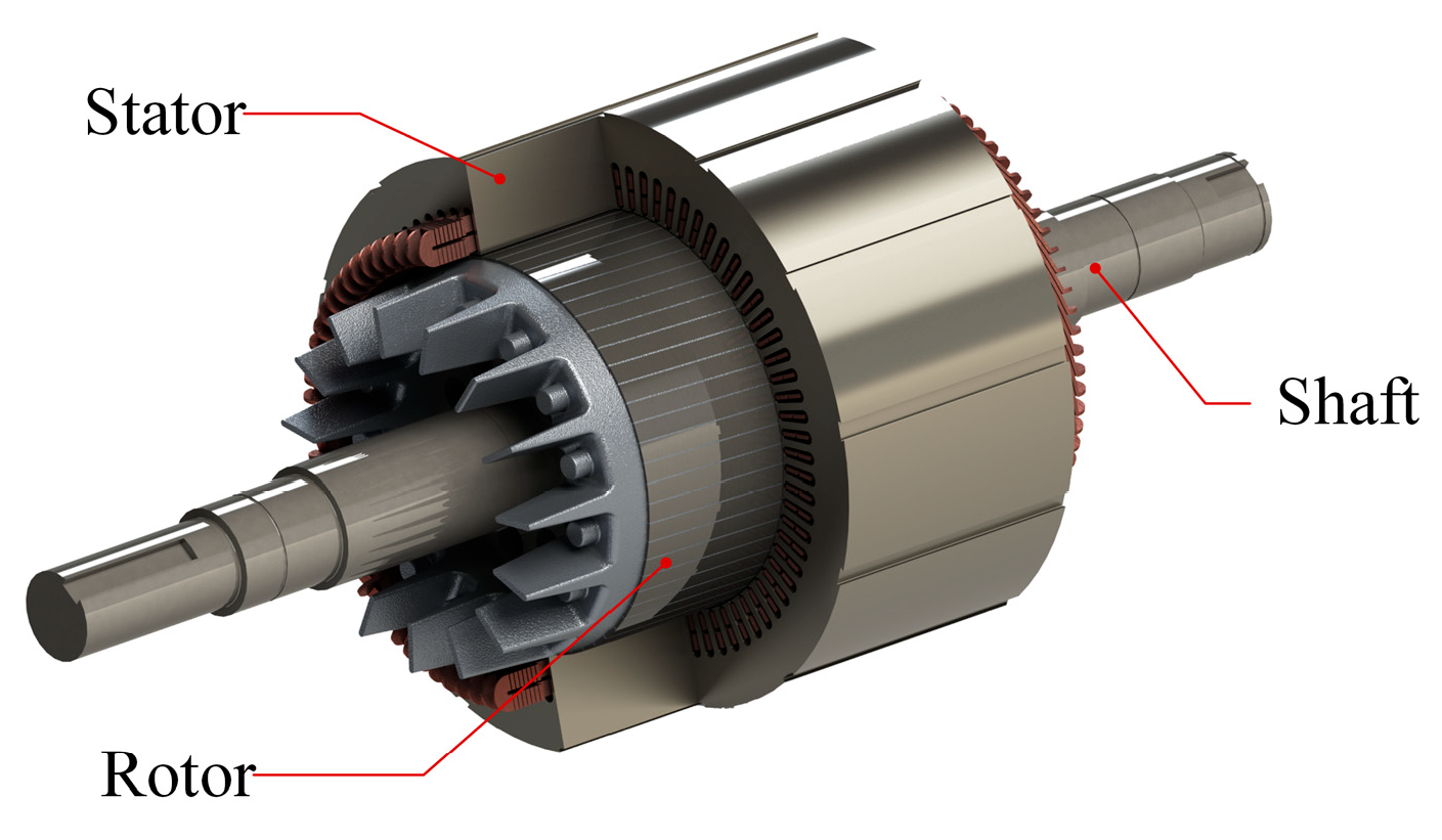
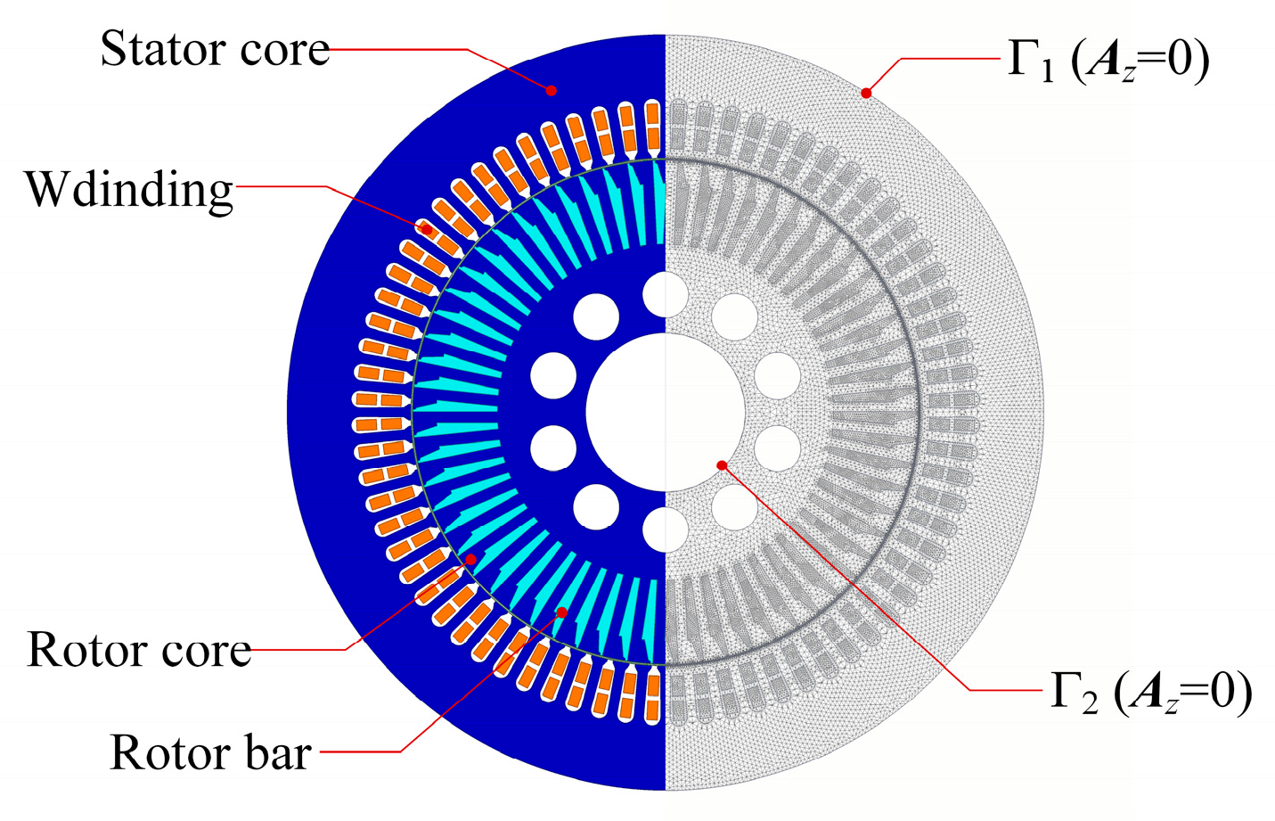
A 160 kW three-phase induction motor is selected to drive the pump. Induction motors are widely used in industrial applications due to their reliable operation and excellent starting and overload capabilities. The structure of the motor is shown in Figure 3, and its main parameters are listed in

Table 2. Main parameters of the induction motor.

Parameter	Value	Unit	Parameter	Value	Unit
Rated power	160	kW	Iron core length	395	mm
Rated voltage	380	V	Air-gap length	1.3	mm
Rated current	285	A	Stator outer diameter	520	mm
Rated speed	1490	rpm	Stator inner diameter	350	mm
Frequency	50	Hz	Rotor inner diameter	110	mm
Poles number	4		Connection type	Δ

. The motor consists of a stator with three-phase windings and a cast-aluminum squirrel-cage rotor. The pump and the motor are connected through a gear reducer.

3. Transient Coupled Dynamics Model

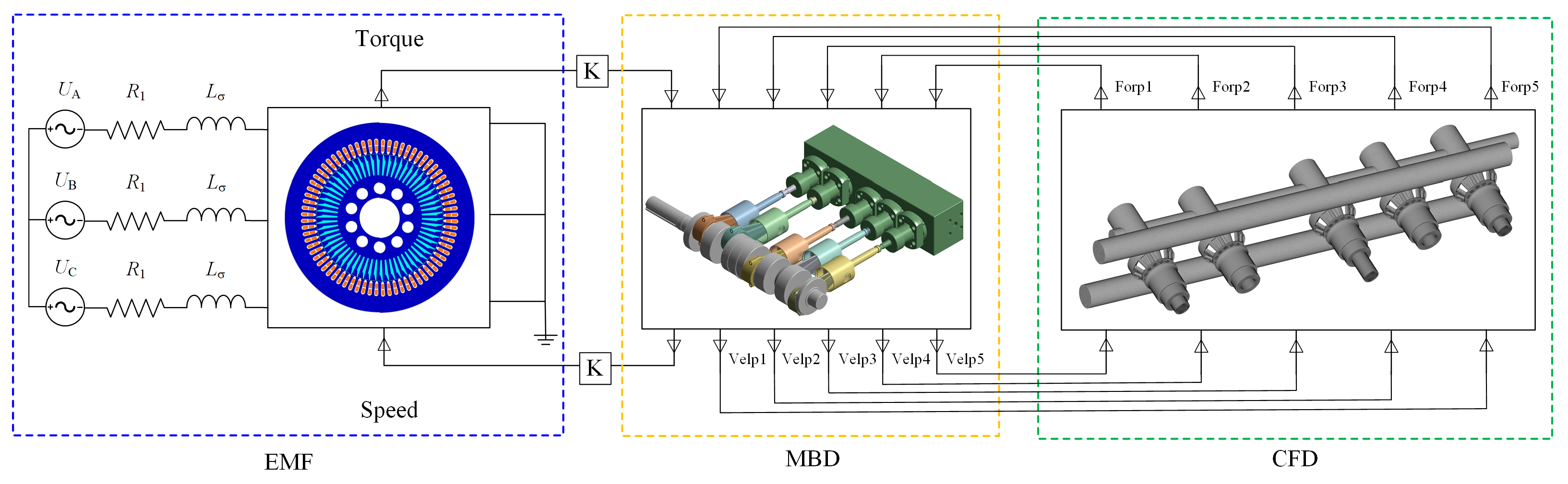
To investigate the interaction mechanisms in a motor–pump system, an electrical–mechanical–hydraulic coupled transient dynamics model is developed. The induction motor is modeled using a two-dimensional (2D) time-stepping finite element method to evaluate its electromagnetic characteristics. 3D CFD is employed to compute the valve motion and fluid flow, while MBD is used to solve the motion of the crankshaft and plungers. The different modules are dynamically coupled through the exchange of forces, torques, velocities, and displacements.

3.1. Electromagnetic Field Model

Neglecting end effects, the induction motor can be modeled using a 2D transient electromagnetic field approach. The electromagnetic field satisfies the following governing equation:

$$\left\{\begin{array}{l}{\displaystyle \frac{\partial }{\partial x}}\left({\displaystyle \frac{1}{{\mu }_p}}{\displaystyle \frac{\partial A_z}{\partial x}}\right)+{\displaystyle \frac{\partial }{\partial y}}\left({\displaystyle \frac{1}{{\mu }_p}}{\displaystyle \frac{\partial A_z}{\partial y}}\right)=-\left(J_z-\sigma {\displaystyle \frac{\mathrm{d}{A}_z}{\mathrm{d}t}}\right)\\ {\left.A_z\right|}_{{\mathrm{\Gamma }}_1}={\left.A_z\right|}_{{\mathrm{\Gamma }}_2}=0\end{array}\right.$$

(1)

where $A_z$ is the z-direction component of the magnetic vector potential, ${\mu }_p$ is the permeability, $J_z$ is the z-direction component of the current density, $\sigma$ is the electrical conductivity, $t$ is the time.

The finite element model and mesh are shown in Figure 4. The stator windings are excited via an external circuit. Dirichlet boundary conditions are applied to the outer boundary of the stator and the inner boundary of the rotor. Exploiting the structural symmetry, a 1/2-sector model is adopted to reduce computational cost, with periodic boundary conditions applied to the cut surfaces. The resistance and leakage inductance of the end windings and end rings are incorporated into the simulation as circuit parameters. A multi-slice method is employed to account for the skewed rotor slots. The effectiveness of the 2D multi-slice FEM model for induction machines with skewed rotors has been demonstrated in a previous study [23].

3.2. Multi-Body Dynamics Model

To analyze the motion of the power end of the plunger pump under various external excitations, an MBD model is established, as shown in Figure 5. Assuming that elastic deformation is negligible, all power-end components are modeled as rigid bodies. In this model, components connected by screws are simplified as a single part or treated with fixed constraints. Bearings and bearing shells are neglected, and the hydraulic end is considered a fixed component, serving only to restrict the motion of the plungers. The materials and masses of the movable parts of the pump are listed in

Table 3. Materials and masses of the movable components of the pump.

Component	Material	Density (g/cm3)	Mass (kg)
Crankshaft	40Cr	7.85	320.4
Connecting rod	ZG340~640		14.98
Link rod	45#		4.080
Plunger	45#		2.644
Crosshead	HT250	7.15	14.91

.

The components are connected through kinematic pairs, with all surface contacts assumed to be frictionless. The motion of the system is governed by the constrained Lagrange equations:

$$\left\{\begin{array}{l}\mathit{M}\ddot{\mathit{q}}+{\mathbf{\Phi }}_q^T\mathit{\lambda }+\mathit{F}(\mathit{q})=\mathit{Q}(\mathit{q})\\ \mathbf{\Phi }(\mathit{q},t)=0\end{array}\right.$$

(2)

where $\mathit{M}$ is the mass matrix, $\mathit{q}$ is the degrees of freedom of the system, $\mathit{\lambda }$ is the Lagrange multiplier, $\mathit{F}(\mathit{q})$ is the internal forces of the system, $\mathit{Q}(\mathit{q})$ is the generalized external forces, $\mathbf{\Phi }(\mathit{q},t)$ is the constraint function. The load acting on the power end consists of the torque transmitted from the motor via the reducer and the hydraulic pressure acting on the plunger surface. The joints between different components are listed in

Table 4. Types of joints between different pump components.

Component	Joint
Crankshaft and ground	Revolute
Crankshaft and connecting rod	Revolute
Connecting rod and crosshead	General
Plunger and hydraulic end	Translational
Crosshead and link rod	Fixed
link rod and plunger	Fixed
Hydraulic end and ground	Fixed

.

3.3. Computational Fluid Dynamics Model

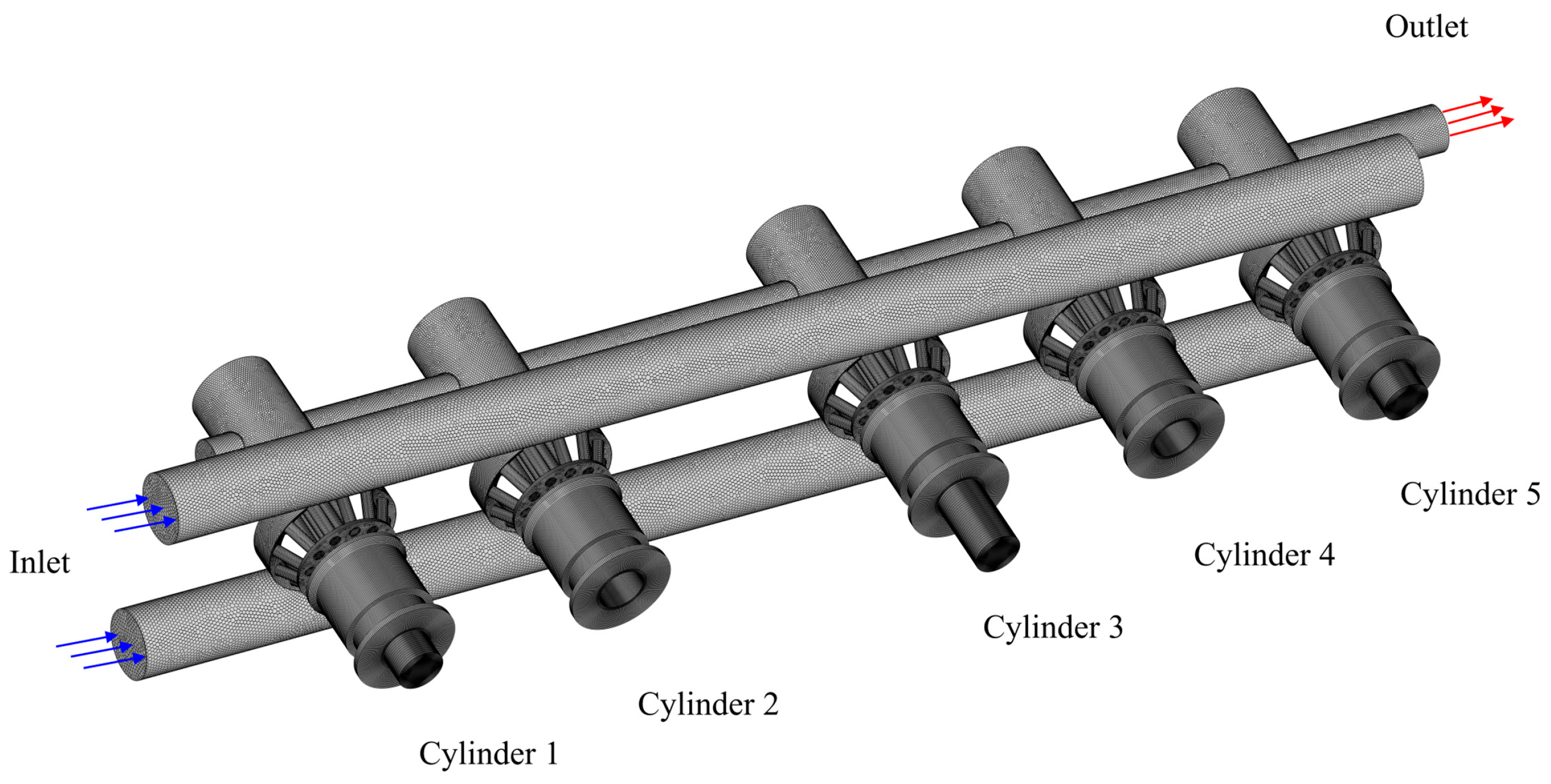
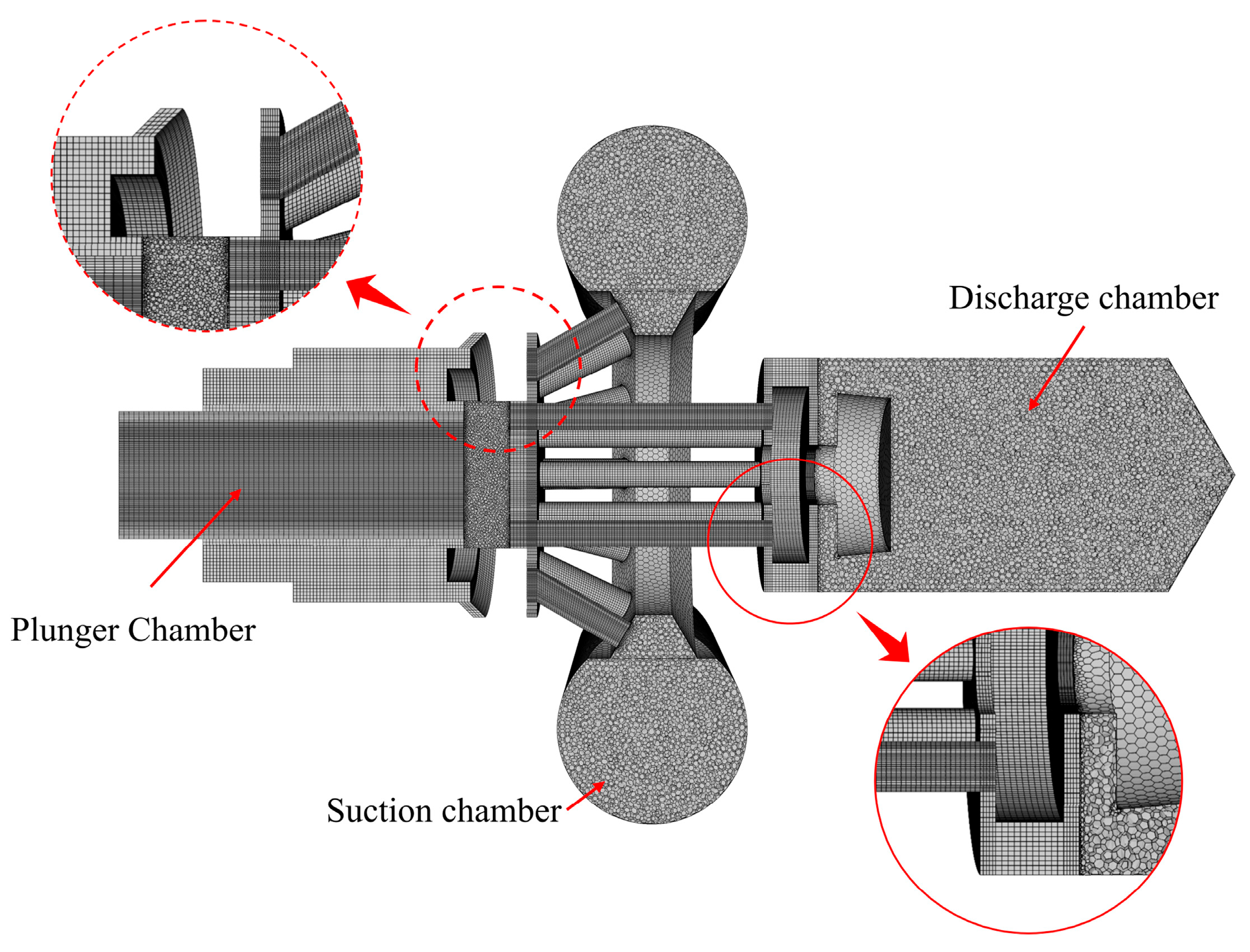
After simplifying certain geometric features, such as chamfers, filets, studs, and springs, the fluid domain was extracted to establish a 3D CFD model, as shown in Figure 6. Figure 7 shows the cross section of the fluid domain for a single cylinder.

The fluid in the computational domain satisfies mass conservation and momentum conservation. The Navier–Stokes equations governing the fluid flow can be written as [24]

$${\displaystyle \frac{\partial \rho }{\partial t}}+\nabla \cdot (\rho \mathit{v})=0$$

(3)

$${\displaystyle \frac{\partial }{\partial t}}(\rho \mathit{v})+\nabla \cdot (\rho \mathit{v}\mathit{v})+\nabla p-\nabla \cdot \mathit{\tau }=0$$

(4)

where $\rho$ is the density of the fluid, $\mathit{v}$ is the velocity vector, $p$ is the pressure, $\mathit{\tau }$ is the stress tensor. The $\mathit{\tau }$ can be further expressed as

$$\mathit{\tau }=\nabla \cdot \left[\mu \left(\nabla \mathit{v}+{(\nabla \mathit{v})}^T\right)\right]+\nabla \left(\lambda \nabla \cdot \mathit{v}\right)\mathit{I}$$

(5)

where $\mu$ is the molecular viscosity, $\lambda$ is the bulk viscosity coefficient, and $\mathit{I}$ is the unit tensor.

To apply the finite volume method, the fluid domain was discretized into a large number of hexahedral and polyhedral elements, as shown in Figure 6 and Figure 7. Structured hexahedral meshes were generated for regular geometries, whereas polyhedral meshes were adopted for irregular regions. The interface between the moving and stationary meshes was defined as a non-conformal mesh interface to facilitate data transfer across non-matching grids.

The SST k-ω model is used for turbulence modeling to capture the turbulent flow characteristics. It offers improved accuracy across a wide range of flow regimes, especially in cases involving strong adverse pressure gradients and flow separation. The transport formulation of the SST k-ω model is expressed as [25]

$$\left\{\begin{array}{l}{\displaystyle \frac{\partial }{\partial t}}(\rho k)+\nabla \cdot \left(\rho k\mathit{v}\right)=\nabla \cdot \left[\left(\mu +{\displaystyle \frac{{\mu }_t}{{\sigma }_k}}\right)\nabla k\right]+G_k-Y_k+S_k+G_b\hfill \\ {\displaystyle \frac{\partial }{\partial t}}(\rho \omega )+\nabla \cdot \left(\rho \omega \mathit{v}\right)=\nabla \cdot \left[\left(\mu +{\displaystyle \frac{{\mu }_t}{{\sigma }_{\omega }}}\right)\nabla \omega \right]+G_{\omega }-Y_{\omega }+D_{\omega }+S_{\omega }+G_{\omega b}\hfill \end{array}\right.$$

(6)

In the equations, $k$ is the turbulent kinetic energy; $\omega$ is the specific dissipation rate; ${\mu }_t$ is the turbulent viscosity; ${\sigma }_k$ and ${\sigma }_{\omega }$ are the turbulent Prandtl numbers for $k$ and $\omega$; $G_k$ and $G_{\omega }$ represent the generation of turbulence kinetic energy and specific dissipation; $Y_k$ and $Y_{\omega }$ represent the dissipation of $k$ and $\omega$; $D_{\omega }$ represents the cross-diffusion term; $S_k$ and $S_{\omega }$ are user-defined source terms; $G_b$ and $G_{\omega b}$ represent the buoyancy terms. The unique feature of the SST k-ω model is the introduction of a limiter to the formulation of the turbulent viscosity.

The detailed solver settings are listed in

Table 5. Solver settings.

Setting	Parameters	Type	Valve
Solver	Pressure-based model
Materials	Fluid	Liquid water (compressible)
Solution Methods	Pressure velocity couple	PISO
	Spatial discretization	Pressure	PRESTO!
		Density	Second-order upwind
		Momentum	Second-order upwind
Turbulence model	SST k-omega
Boundary condition	inlet	Pressure	0.1 MPa
	outlet	Pressure	37 MPa

.

Dynamic meshing is used to depict the movement at the boundaries of the fluid domain caused by the motion of the plungers and valves. The velocity of the plungers is determined by an MBD model, whereas the velocity of the valves is obtained by solving their motion equations. The suction and discharge valves periodically open and close under the action of spring, hydraulic, and damping forces. Therefore, the valve motion equation can be written as

$$m{\displaystyle \frac{d^{2}x}{d{t}^2}}+c{\displaystyle \frac{dx}{dt}}=k_s(x+x_0)+A_{val}\mathrm{\Delta }p$$

(7)

where $m$ is the mass of the valve, $x$ is the displacement, $c$ is the damping coefficient, $k_s$ is the spring stiffness, $A_{val}$ is the surface area of the valve, $\mathrm{\Delta }p$ is the pressure difference.

The valve dynamics are solved using User-Defined Functions (UDFs), which store all required variables and parameters. At each time step, the hydraulic force acting on the valve is obtained by integrating the pressure over the valve surfaces. The spring and damping forces are then evaluated from the current valve displacement and velocity. These forces are substituted into (7), and a fourth-order Runge–Kutta method is employed as the numerical differentiation scheme. The time step of the Runge–Kutta scheme is fixed at 0.05 times the global time step. If the valve reaches its mechanical limits, corresponding constraints are imposed on its displacement and velocity. The updated valve motion is subsequently used to regenerate the mesh, after which the flow field is solved. This procedure is repeated for successive time steps until the end of the simulation.

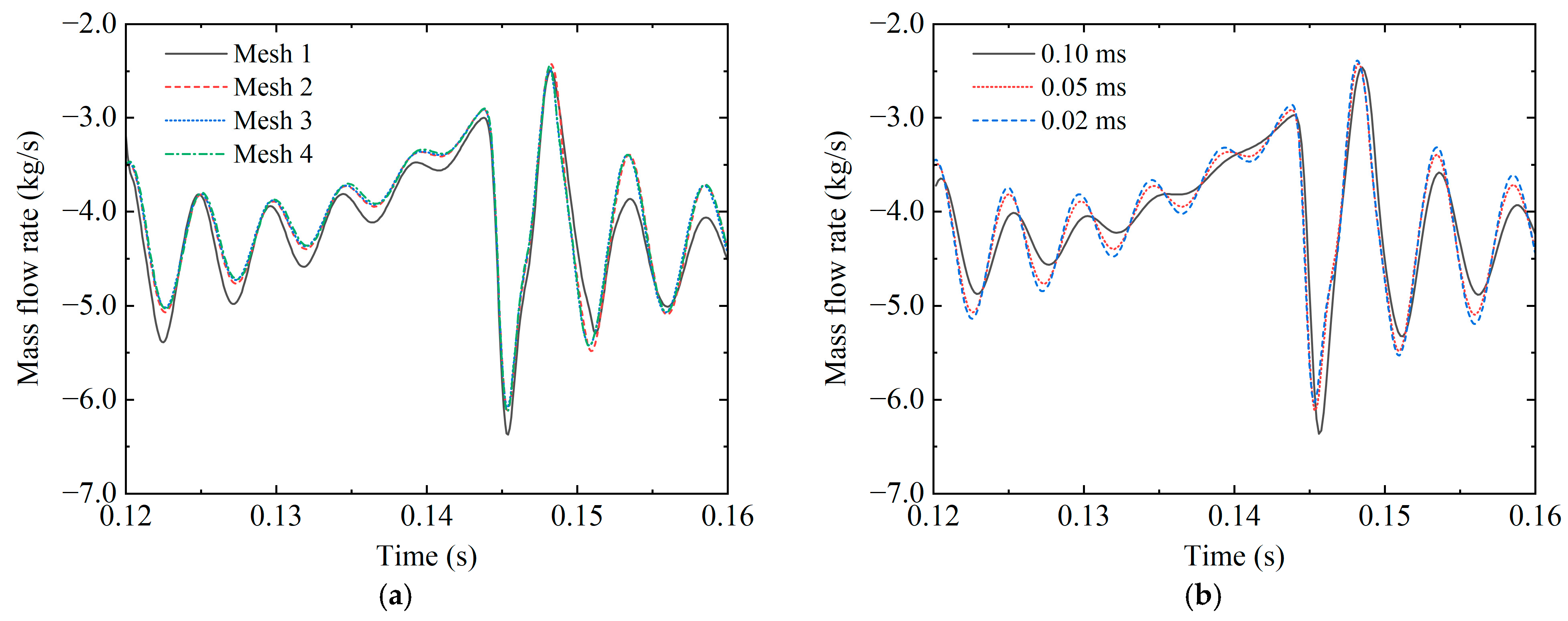
To eliminate the influence of mesh size and time step on the numerical results, mesh independence and time-step sensitivity analyses were conducted. Figure 8a presents the outlet mass flow rate obtained using four different mesh sizes. Meshes 1–4 consist of 4,054,560, 6,871,237, 8,652,342, and 10,284,002 cells, respectively. It can be observed that, as the number of cells increases, the flow rate curves exhibit a clear convergence trend. Taking Mesh 4 as the reference, the relative root mean square errors of Meshes 1–3 are 5.325%, 1.293%, and 0.774%, respectively. Considering the balance between computational accuracy and cost, Mesh 2 is selected for the final mesh scheme.

Figure 8b shows the outlet mass flow rate obtained using three different time steps of 0.1 ms, 0.05 ms, and 0.02 ms. Taking the time step of 0.02 ms as the reference, the relative root mean square errors of the other two cases are 5.233% and 1.437%, respectively. The deviation between the results obtained with 0.05 ms and 0.02 ms is less than 2%; therefore, a time step of 0.05 ms is selected for subsequent simulations.

3.4. Coupled Solution

A transient coupled simulation model is established using commercial software packages, including Ansys Twin Builder 2024 R1 (system coupling), Ansys Electronics Desktop 2024 R1 (FEM), Ansys Fluent 2024 R1 (CFD), and Ansys Motion 2024 R1 (MBD), as shown in Figure 9. The different physical fields are coupled through the exchange of forces, torques, displacements, and velocities. Under the assumption of an ideal three-phase power supply, the electromagnetic field is solved to obtain the torque based on the instantaneous rotor speed, which is provided by the rigid-body dynamics model. The induction machine and the pump are mechanically linked through the gear reducer, resulting in constant torque and speed transmission ratios. These ratios are accounted for by introducing a linear proportionality coefficient. Based on the torque on the crankshaft and the forces on the plungers, the crankshaft rotational speed and plunger velocities are determined using an MBD model. The plunger displacement is employed to determine the movement of the fluid boundary. The valve motion is implemented using UDFs in the model. The solution of the flow field provides the hydraulic forces acting on the surfaces of the plungers and valves, which are then transferred to the MBD model as input.

4. Results and Discussion

4.1. Electromagnetic Characteristics

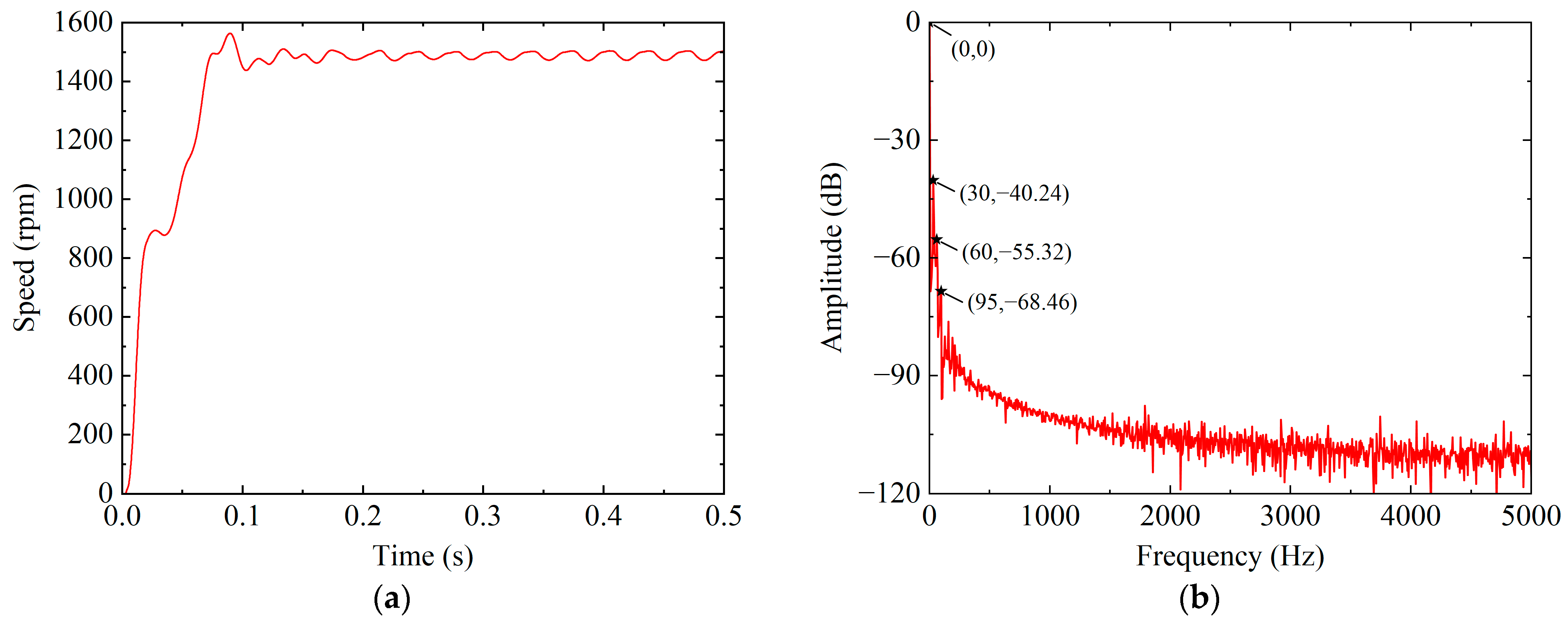
The proposed model is used to evaluate the dynamic characteristics of the motor–pump coupled system. The simulation is performed for a total time of 0.5 s with a time step of 0.1 ms. Figure 10 presents the curve of the motor rotational speed and its spectrum. During the start-up phase, the motor speed increases continuously and stabilizes after transient oscillations. Due to the periodic load torque, noticeable fluctuations in the motor rotational speed are present. The fluctuation coefficient is defined as:

$${\delta }_n={\displaystyle \frac{n_{\max }-n_{\min }}{n_{\mathrm{mean}}}}\times 100\%$$

(8)

where $n_{\max }$, $n_{\min }$, $n_{\mathrm{mean}}$ are maximum value, minimum value, and mean value of the rotational speed, respectively, and the ${\delta }_n$ is 2.11%.

The speed data from 0.3 s to 0.5 s are analyzed using FFT. Because the amplitude of the speed spectrum varies significantly, it is converted to a decibel scale. In the speed spectrum, the 0 dB corresponds to a constant-speed component at 0 Hz, whose amplitude is 1489.93 rpm. Moreover, three oscillatory components are observed at frequencies of 30 Hz, 60 Hz, and 95 Hz. Their actual amplitudes are 12.93 rpm, 2.30 rpm, and 1.05 rpm, corresponding to 0.87%, 0.15%, and 0.07% of the constant component, respectively. The pulsation frequencies are associated with the reciprocating frequency of the pump and its harmonics. The reciprocating frequency of the pump can be expressed as follows:

$$f_r={\displaystyle \frac{nN}{60i}}$$

(9)

where $n$ is the rotational speed of the motor, $N$ is the number of plungers, $i$ is the reduction ratio. Consequently, the curves of $n$ and $f_r$ have the same shape. The mean value of $f_r$ is 31.01 Hz. Since FFT cannot accurately capture continuously varying frequencies, the obtained result is only an approximation.

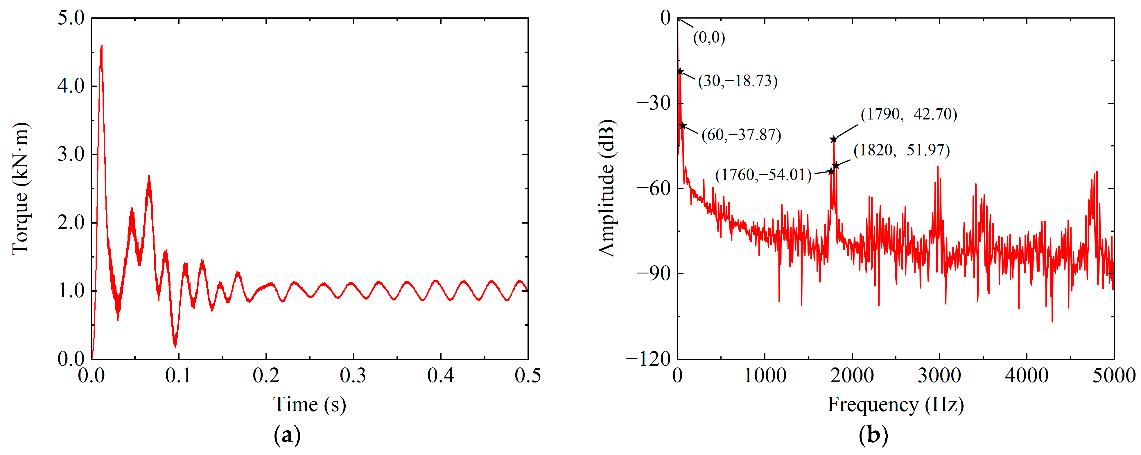
Figure 11 shows the instantaneous torque of the motor and its spectrum. Due to direct starting, the motor torque rises rapidly to 4.5 kN·m at the start. Subsequently, the torque decreases and undergoes fluctuations lasting approximately 0.2 s before stabilizing. According to (8), the torque fluctuation coefficient is 29.57%. In the torque spectrum, the actual amplitude of the constant torque components corresponding to 0 dB is 1.015 kN·m. Similar to the rotational speed spectrum, the torque spectrum mainly consists of components at 30 Hz and 60 Hz. The amplitudes of these components are 0.107 kN·m and 0.010 kN·m, corresponding to 10.54% and 0.99% of the constant torque amplitude, respectively. Additionally, the components at 1790 Hz and 1790 ± 30 Hz are observed in the torque spectrum. The component at 1790 Hz is derived from the harmonic magnetic field in the air gap of the motor, whereas the components at 1790 ± 30 Hz are correlated with the reciprocating frequency of the pump.

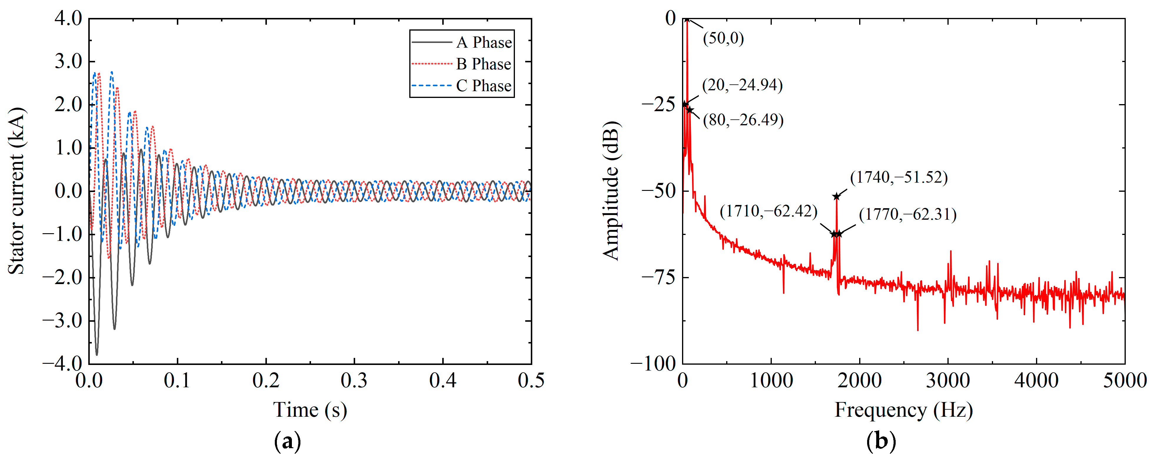
The fluctuations caused by the periodic load are also reflected in the stator current. Figure 12 shows the instantaneous stator current of the motor and its spectrum. The motor exhibits a significant start-up current. The actual amplitude of the fundamental current at 50 Hz is 221.14 A. In addition to the fundamental component at 50 Hz, sideband components at 20 Hz and 80 Hz are observed, which are exactly equal to $50\pm f_r$. Similarly, the components at 1740 ± 30 Hz can be observed near the component at 1740 Hz. Therefore, pump load can modulate the original fundamental and harmonic components and induce extra sideband harmonic components in the speed, torque and current spectrum.

4.2. Valve Motion and Fluid Flow Characteristics

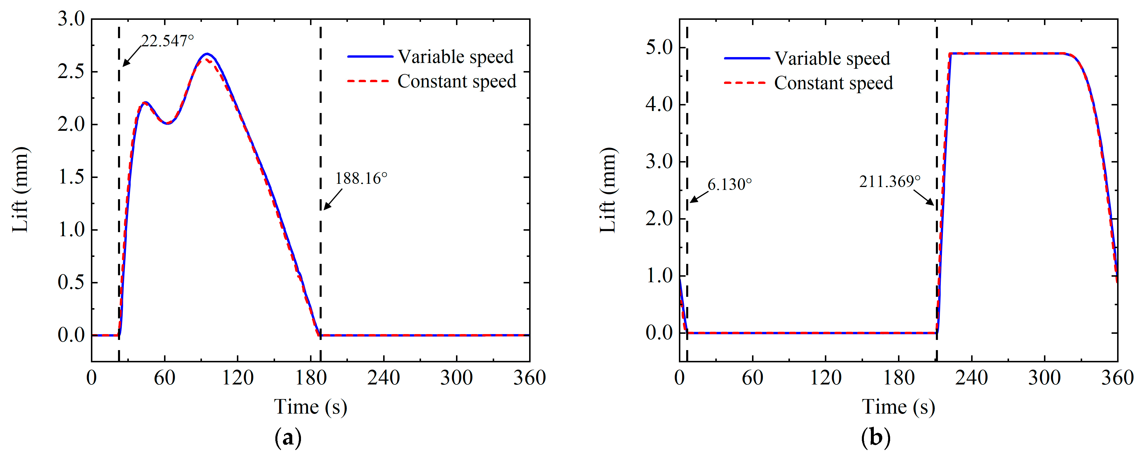
Figure 13 shows the lift curves of the suction and discharge valves under constant-speed and variable-speed conditions. Under the constant-speed condition, the crankshaft speed is set to 370 rpm. Under the variable-speed condition, the rotational speed is determined by the coupled motor–pump system. The time axis is converted to the crank angle based on the rotational speed of the crankshaft. Taking the third cylinder block as the reference, 0–180° corresponds to the suction stroke, while 180–360° corresponds to the discharge stroke. When the lift is 0, it indicates that the valve is in the closed position. By comparing the results for the two cases, it can be observed that the valve motion patterns in the two cases are almost identical. Due to the relatively small fluctuations in rotational speed, the electromagnetic characteristics exert only a limited influence on the valve motion. After the start of the suction stroke, the suction valve begins to open rapidly at 22.55°. The lift then slightly decreases before reaching a maximum value of approximately 2.670 mm. Subsequently, the valve gradually closes and becomes fully closed at 188.16°. Due to the compressibility of the fluid, the discharge valve does not open immediately after the suction valve closes. As the plunger moves, the pressure in the plunger chamber increases continuously. The valve opens only when the fluid pressure exceeds the spring force. When the crank angle reaches 211.37°, the discharge valve opens rapidly and reaches its maximum lift. After a period of time, it begins to close and becomes fully closed at 6.130° in the next stroke.

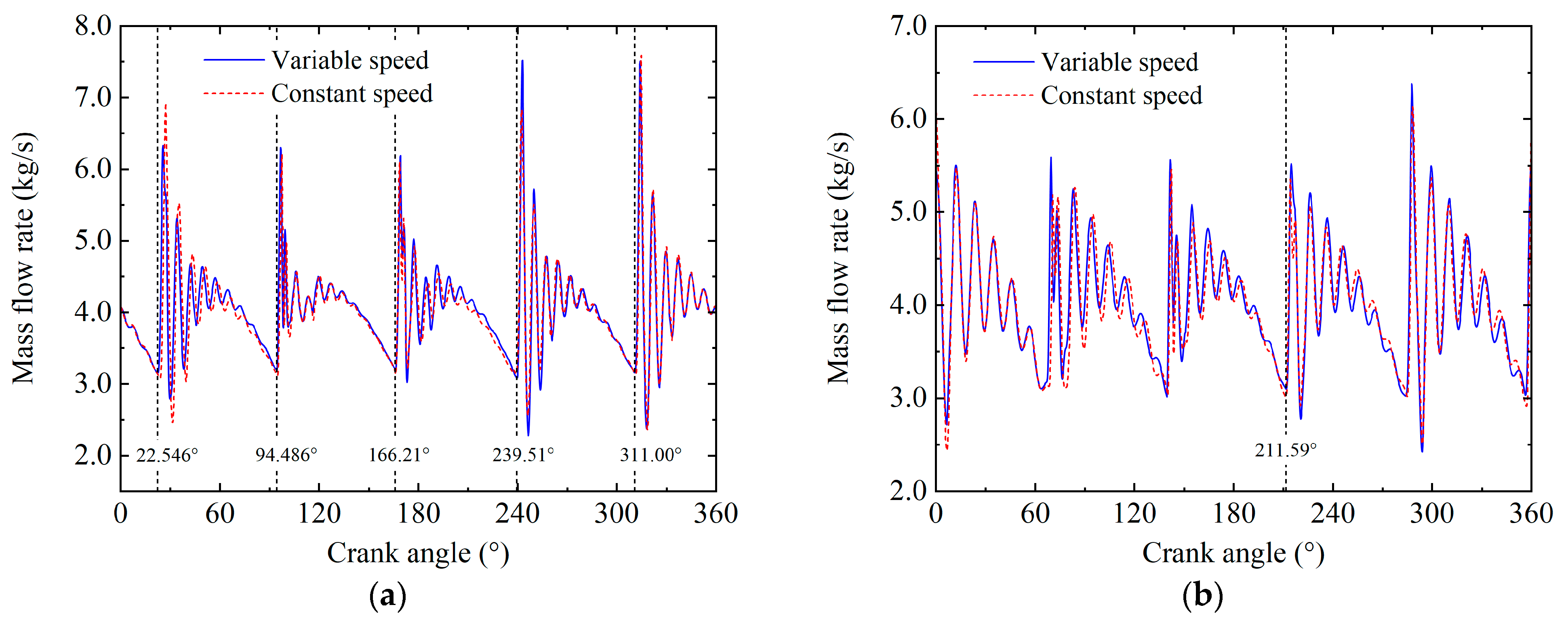
Figure 14 shows the inlet and outlet mass flow rate curves. Under both constant-speed and variable-speed conditions, the overall trends of the flow rate curves are nearly identical, with only minor differences. In the variable-speed case, the average suction and discharge mass flow rates are 4.046 and 4.047 kg/s, respectively, whereas in the constant-speed case, they are both 4.019 kg/s. In addition, five distinct main peaks can be identified in the flow curves, and the phase difference between adjacent peaks is approximately 72°. When the suction valve opens, the pressure in the plunger chamber is lower than that in the suction chamber. Due to the presence of inertia, the fluid will not be sucked into the plunger chamber until a brief delay, resulting in a small pressure fluctuation in the pressure within the plunger chamber. As the suction valve opens further, a large amount of fluid will be drawn in. As the pressure fluctuations gradually diminish, the flow pulsations will also gradually decrease until the suction valve of the next cylinder opens. Similar phenomena can also be observed in the discharge flow curve.

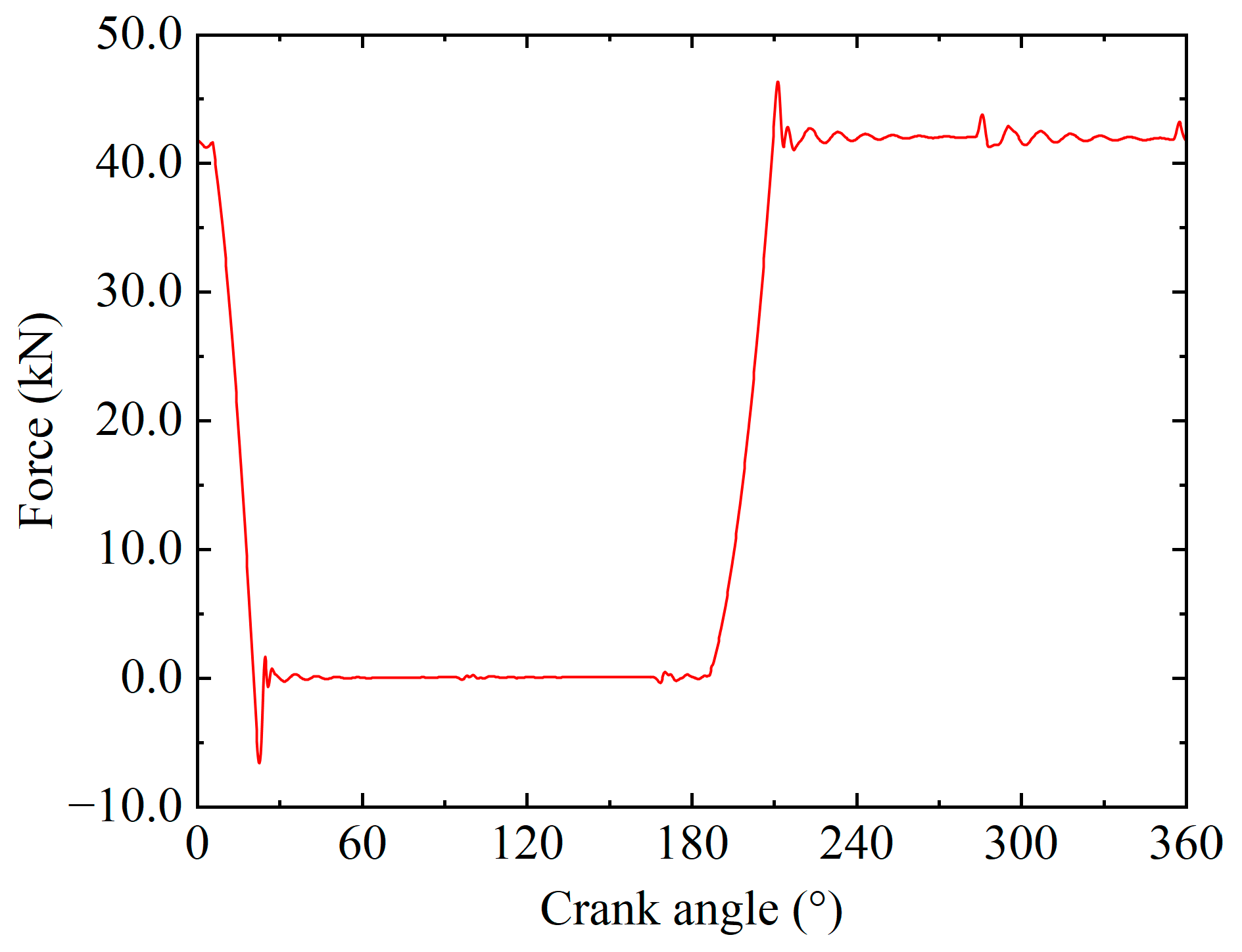
Figure 15 illustrates the hydraulic force acting on the end face of the plunger in Cylinder 3. Since the effective area of the plunger end face is constant, the force variation is proportional to the pressure variation in the plunger chamber. During the suction stage, the hydraulic force on the plunger remains close to zero. During the discharge stage, the chamber pressure rises rapidly, producing a hydraulic force of approximately 42 kN. Small transient force peaks occur during each transition between the suction and discharge strokes. In addition, a slight force fluctuation is observed at a shaft angle of approximately 285.55°, which coincides with the discharge valve reaching its maximum lift. The subsequent rapid valve closure may induce a weak water-hammer effect in the plunger chamber.

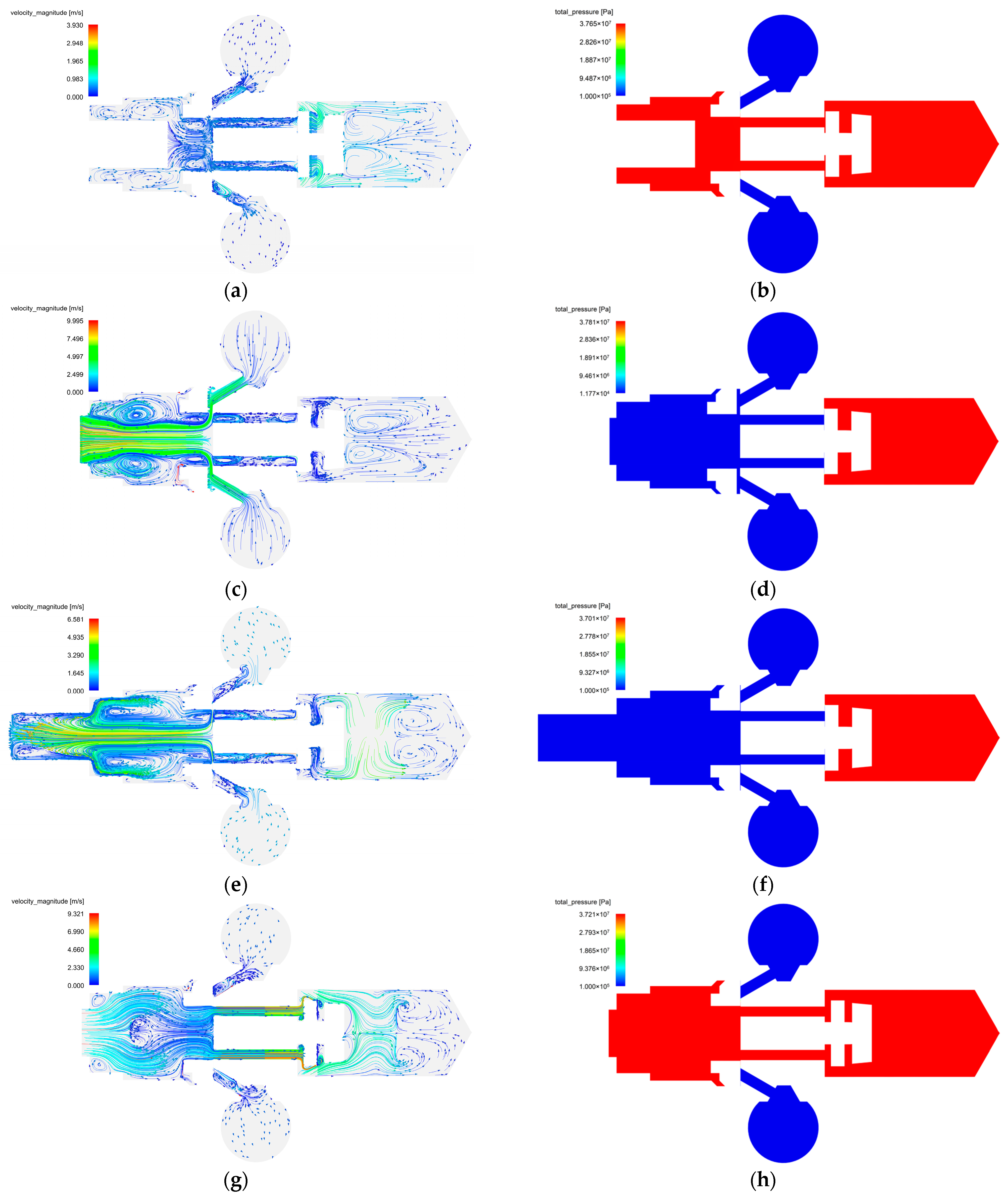
To further reveal the pump flow characteristics, Figure 16 presents the velocity vector field and pressure distribution in Cylinder 3 at crank angles of 0°, 90°, 180°, and 270°. When the crank angle is 0°, the discharge stroke has just ended, and only a small amount of flow passes through the discharge valve clearance. As the discharge valve is closing rapidly, the near-wall fluid is entrained and moves with the valve. The pressure contours indicate that the pressure in the plunger chamber is approximately 37 MPa at this crank angle, and the peak pressure slightly exceeds 37 MPa. A significant pressure gradient is observed near the suction valve seat.

When the crank angle is 90°, the pump is halfway through the suction stroke, and a large inflow rate is drawn into the plunger chamber. It can be seen that the pronounced velocity difference between the high-speed core flow at the chamber center and the slower near-wall fluid induces strong shear; as a result, the fluid in the clearance volume interacts with the main flow, and recirculation vortices form. At this crank angle, the pressure in the plunger chamber is approximately 0.1 MPa, and the minimum pressure drops slightly below 0.1 MPa.

When the crank angle is 180°, the pressure in the plunger chamber is approximately 0.1 MPa. The suction stroke has just ended, but the suction valve has not yet fully closed. Due to fluid inertia, the flow still tends to enter the chamber.

When the crank angle is 270°, the pressure in the plunger chamber is approximately 37 MPa, and a large flow rate is discharged at this stage. Owing to the rapid reduction in the diameter of the plunger chamber, a distinct recirculating flow can be observed in the central region of the chamber.

5. Conclusions

This study develops a transient coupled dynamic model of a motor–pump system and investigates its electrical–mechanical–hydraulic coupling characteristics under transient conditions. The results show that the alternating suction and discharge processes induce periodic rotational-speed fluctuations at the pump reciprocating frequency. Under these speed pulsations, the motor generates torque ripple components at the reciprocating frequency and its harmonics. Meanwhile, sidebands spaced by the reciprocating frequency appear in the stator current spectrum. Valve-motion analysis reveals significant delays in both valve opening and closing. The closing delay is mainly governed by valve parameters, whereas the opening delay is influenced by the closing delay as well as fluid compressibility. Flow-field analysis shows that, during the suction stroke, the velocity difference between the high-speed core flow and the near-wall fluid generates pronounced vortices in the residual clearance of the plunger chamber. During the discharge stroke, vortices also form in the midsection of the plunger chamber due to a locally enlarged diameter. By comparing valve motion and flow characteristics under constant-speed and variable-speed conditions, it is found that speed fluctuations induced by the electromagnetic characteristics of the motor only have a limited effect on the hydraulic performance of the pump.

The proposed modeling framework has broad application potential. Its complexity can be adjusted according to different research objectives. A limitation of this study is the lack of experimental validation. Improving the model accuracy will be a key focus of future work. Experimental comparisons will be conducted to further validate the proposed model.

References

1. Josifovic, A.; Roberts, J.J.; Corney, J.; Davies, B.; Shipton, Z.K. Reducing the environmental impact of hydraulic fracturing through design optimisation of positive displacement pumps. Energy 2016, 115, 1216–1233. [Google Scholar] [CrossRef] [Scilit]
2. Li, R.; Wei, W.; Lai, Y.; Lu, H.; Cao, T.; Ye, J.; Liu, H. Experimental and numerical study on valve dynamic impact contact characteristics and fault diagnosis of a reciprocating piston pump. Sci. Prog. 2025, 108, 1–20. [Google Scholar] [CrossRef] [Scilit]
3. Cieślicki, R.; Karpenko, M. An investigation of the impact of pump deformations on circumferential gap height as a factor influencing volumetric efficiency of external gear pumps. Transport 2022, 37, 373–382. [Google Scholar] [CrossRef] [Scilit]
4. Aakre, S.R.; Anderson, M.H.; Brook, P.W. Volumetric efficiency and pressure pulsations of a triplex reciprocating supercritical CO2 pump. J. Supercrit. Fluids 2021, 168, 105072. [Google Scholar] [CrossRef] [Scilit]
5. Wang, T.; Wang, G.; Dai, L.; Chen, L.; Qiu, S.; Li, R. Motion mechanism study on the valve disc of an ultra-high pressure reciprocating pump. Mech. Syst. Signal Process. 2021, 160, 107942. [Google Scholar] [CrossRef] [Scilit]
6. Ma, Y.; Ni, Y.; Zhang, H.; Zhou, S.; Deng, H. Influence of valve’s lag characteristic on pressure pulsation and performance of reciprocating multiphase pump. J. Pet. Sci. Eng. 2018, 164, 584–594. [Google Scholar] [CrossRef] [Scilit]
7. Zhu, G.; Dong, S. Analysis on the performance improvement of reciprocating pump with variable stiffness valve using CFD. J. Appl. Fluid Mech. 2020, 12, 387–400. [Google Scholar] [CrossRef] [Scilit]
8. Gu, Z.; Bai, C.; Zhang, H. Dynamic modeling of reciprocating pump valves with considering the interaction effects between pump and pipeline. Proc. Inst. Mech. Eng. Part I J. Syst. Control Eng. 2022, 236, 1491–1502. [Google Scholar] [CrossRef] [Scilit]
9. Zhao, S.; Tang, H.; Ren, Y.; Wu, D.; Liu, Y. The attitude changes and leakage characteristics of large-scale plunger pairs in high-pressure plunger pumps. Flow Meas. Instrum. 2025, 102, 102838. [Google Scholar] [CrossRef] [Scilit]
10. Dong, J.; Liu, Y.; Ji, H.; Wei, L.; Wu, D. Simulation of unsteady flow characteristics of the reciprocating pump check valve for high pressure and high flow water medium. J. Fluids Eng. 2022, 144, 031206. [Google Scholar] [CrossRef] [Scilit]
11. Qiu, G.; Zhu, S.; Wang, K.; Wang, W.; Hu, J.; Hu, Y.; Zhi, X.; Qiu, L. Numerical study on the dynamic process of reciprocating liquid hydrogen pumps for hydrogen refueling stations. Energy 2023, 281, 128303. [Google Scholar] [CrossRef] [Scilit]
12. Munsch, P.; Kiermerir, J.; Schilling, R.; Schluecker, E.; Skoda, R. Three-dimensional simulation of cavitation flow in reciprocating positive displacement pumps with fluid-actuated valves. ASEM J. Fluid Eng. 2025, 147, 041201. [Google Scholar] [CrossRef] [Scilit]
13. Munsch, P.; Gianfelice, T.; Feist, M.; Schlücker, E.; Skoda, R. Three-dimensional/one-dimensional seamlessly coupled simulation of cavitating flow in reciprocating positive displacement pumps and their piping. Phys. Fluids 2025, 37, 025228. [Google Scholar] [CrossRef] [Scilit]
14. Su, G.; Guo, Y.; Deng, H.; Hu, K.; Wang, P.; Wang, S.; Cheng, G. Pulsation analysis and suppression study of pump-controlled motor system driven by variable frequency permanent magnet synchronous motor. Proc. Inst. Mech. Eng. Part C J. Mech. Eng. Sci. 2022, 236, 12. [Google Scholar] [CrossRef] [Scilit]
15. Szolc, T.; Konowrocki, R.; Michajlow, M.; Pregowska, A. An investigation of the dynamic electromechanical coupling effects in machine drive systems driven by asynchronous motors. Mech. Syst. Signal Process. 2014, 49, 118–134. [Google Scholar] [CrossRef] [Scilit]
16. Chen, Y.; Xu, W.; Liu, Y.; Bao, Z.; Mao, Z.; Rashad, E.M. Modeling and transient response analysis of doubly-fed variable speed pumped storage unit in pumping model. IEEE Trans. Ind. Electron. 2023, 70, 9935–9947. [Google Scholar] [CrossRef] [Scilit]
17. Mauri, M.; Rossi, M.; Bruha, M. Generation of torsional excitation in a variable-speed-drive system. In Proceedings of the 2016 International Symposium on Power Electronics, Electrical Drives, Automation and Motion (SPEEDAM), Capri, Italy, 22–24 June 2016. [Google Scholar]
18. Liu, K.; Wu, W.; Yuan, S.; Lu, G.; Chen, X. Modal characteristics of electric vehicle powertrain considering electromagnetic effect. J. Sound Vib. 2022, 530, 116972. [Google Scholar] [CrossRef] [Scilit]
19. Shu, R.; Wei, J.; Tan, R.; Wu, X.; Fu, B. Investigation of dynamic and synchronization properties of a multi-motor driving system: Theoretical analysis and experiment. Mech. Syst. Signal Process. 2021, 153, 107496. [Google Scholar] [CrossRef] [Scilit]
20. Zhao, J.; Zhang, Q.; Wei, X. An integrated approach of a field-circuit coupling model and multi-physics finite-element simulation for analysing transient electromagnetic vibration of pump motors. IET Electr. Power Appl. 2022, 16, 1030–1056. [Google Scholar] [CrossRef] [Scilit]
21. Nan, G.; Chen, E.; Yang, A. Dynamic characteristics of centrifugal pump induced by fluid and motor excitation forces. J. Vibroeng. 2015, 17, 3909–3918. [Google Scholar]
22. Dong, L.; Shuai, Z.; Yu, T.; Jian, J.; Guo, Y.; Li, W. A multi-field coupling simulation model for the centrifugal pump system. Mech. Ind. 2023, 24, 9. [Google Scholar] [CrossRef] [Scilit]
23. Wang, Y.; Shen, T.; Xu, Y. An electromagnetic analytical model of squirrel cage induction motors for transient performance prediction. J. Electr. Eng. Technol. 2025, 20, 3235–3246. [Google Scholar] [CrossRef] [Scilit]
24. Karpenko, M. Aircraft hydraulic drive energy losses and operation delay associated with the pipeline and fitting connections. Aviation 2024, 28, 1–8. [Google Scholar] [CrossRef] [Scilit]
25. Xu, Z.; Xu, Y.; Yang, S.; Wang, Y.; Wang, Y. A novel electromagnetic-thermal-fluid bidirectional coupled model considering multiple factors for temperature rise and loss calculation of high current density motor. Int. J. Therm. Sci. 2026, 220, 110330. [Google Scholar] [CrossRef] [Scilit]
Figure 1. Geometric structure of the plunger pump.
Machines 14 00540 g001
Figure 2. Internal structure of the pump head.
Machines 14 00540 g002
Figure 3. Main structure of the induction motor.
Machines 14 00540 g003
Figure 4. 2D electromagnetic field model and mesh of the induction motor.
Machines 14 00540 g004
Figure 5. Multi-body dynamics model.
Machines 14 00540 g005
Figure 6. Computational fluid domain and mesh.
Machines 14 00540 g006
Figure 7. Mesh of a single cylinder.
Machines 14 00540 g007
Figure 8. Mesh independence and time-step sensitivity analyses. (a) Mesh independence; (b) Time-step sensitivity.
Machines 14 00540 g008
Figure 9. Transient coupled dynamics model for the motor–pump system.
Machines 14 00540 g009
Figure 10. Rotational speed of the induction motor. (a) time-domain waveform; (b) frequency spectrum.
Machines 14 00540 g010
Figure 11. Torque of the induction motor: (a) time-domain waveform; (b) frequency spectrum.
Machines 14 00540 g011
Figure 12. Stator current of the induction motor: (a) time-domain waveform; (b) frequency spectrum.
Machines 14 00540 g012
Figure 13. Valve lift curves: (a) suction valve; (b) discharge valve.
Machines 14 00540 g013
Figure 14. Mass flow rate under constant-speed and variable-speed cases: (a) inlet; (b) outlet.
Machines 14 00540 g014
Figure 15. Hydraulic force acting on the plunger end face.
Machines 14 00540 g015
Figure 16. Velocity vector fields and pressure contours at different crank angles: (a) velocity vector field at θ = 0°; (b) pressure contour at θ = 0°; (c) velocity vector field at θ = 90°; (d) pressure contour at θ = 90°; (e) velocity vector field at θ = 180°; (f) pressure contour at θ = 180°; (g) velocity vector field at θ = 270°; (h) pressure contour at θ = 270°.
Machines 14 00540 g016