A Novel Mechanism Analysis Method for the Robotic Grinding of a TC4 Workpiece Using Acoustic Emission Based on an Improved CCEEMD Algorithm

Abstract

The instantaneous contact zone in robotic abrasive belt grinding involves highly coupled thermo-mechanical interactions between abrasive grains and the workpiece material. Acoustic Emission (AE) signals generated during this process are inherently nonlinear and nonstationary, posing challenges for accurate process monitoring and mechanistic understanding. To address this, this study introduces an innovative AE signal processing framework designed to elucidate the robotic grinding mechanism for Ti-6Al-4V (TC4) titanium alloy. An improved Completely Complementary Ensemble Empirical Mode Decomposition (CCEEMD) algorithm, building upon Empirical Mode Decomposition (EMD), is developed to precisely extract intrinsic mode functions (IMFs) from raw AE data. Subsequently, a novel denoising algorithm utilizing noise statistical characteristics effectively removes invalid noise from the robotic machining system. Validation through robotic grinding experiments on TC4 workpieces successfully established quantifiable relationships between extracted AE features and the underlying grinding mechanism. Significantly, implementing this methodology contributed to extending the effective service life of a structured abrasive belt by approximately 20% while increasing machining efficiency by approximately 12%. This work presents a novel methodology combining improved CCEEMD and statistical denoising for AE analysis in robotic grinding, providing a robust link between AE signatures and material removal mechanisms, ultimately enabling quantitative process optimization.

1. Introduction

Material removal characteristics and mechanisms of compliant grinding remain challenging because the process involves coupled robot compliance, local contact deformation, abrasive belt wear, and thermo-mechanical interactions in the grinding zone, especially for the robotic belt grinding of complex workpieces [1,2,3,4]. Although modern industrial robots can provide high nominal repeatability, robotic grinding still faces precision challenges due to effective stiffness reduction under process loads, local contact deformation, and uneven abrasive belt wear [5,6]. Achieving high-precision closed-loop machining in the robotic grinding of complicated workpieces—a topic that has drawn considerable attention—hinges on precise digital monitoring and grinding mechanisms [7,8,9].

Numerous studies have been conducted from various perspectives to elucidate the material mechanism in conjunction with the intricate machining parameters and material characteristics by monitoring the machining process. In the abrasive belt grinding process, Pandiyan et al. [10] employed acoustic emissions to identify changes in contact mechanisms caused by tool wear and concluded that the cutting mechanism predominates on belt tools with fresh grains, progressively declining as the grain wears. Caesarendra et al. [11] provided an acoustic emission-based technique for monitoring the health of low-speed reversible slew bearings and indicated that AE energy is the most sensitive feature for detecting wear in slew bearings operating at low rotational speeds. By combining the multi-sensor fusion of sound and current signals under varying grinding parameters, Cheng et al. [12] created a Bayesian network to detect the belt wear condition, and the fusion of the sound and current significantly increases the accuracy of the prediction findings from 86% to 95%. Chen and Zhang et al. [13,14] suggested a novel technique based on sound signals to achieve real-time quantitative monitoring of abrasive belt conditions in robotic grinding systems, whose maximum absolute percentage errors (MAXE) are within 14%. In addition to signal-based monitoring, positioning accuracy, process velocity, and energy-consumption behavior are also critical evaluation dimensions for practical robotic manufacturing systems. Recent studies have shown that these factors directly affect production efficiency, process stability, and sustainability performance and should be considered jointly in process-orientated analysis [15].

Due to the complex nonlinear dynamics and numerous process parameters involved in the robotic grinding of complex surface components, the real-time acquisition and accurate processing of acoustic emission (AE) signals are of particular significance for process monitoring and quality prediction. Currently, wavelet transform (WT), Hilbert–Huang transform (HHT), and short-time Fourier transform (STFT) are some of the most used signal time-frequency analysis techniques [16]. In order to create the Hidden Markov Model (HMM) for the sharp and worn tool, Lu et al. [17] first employed fast Fourier transform (FFT) to examine the gathered signals, which achieved microtool wear monitoring. Lin et al. [18] proposed discrete wavelet transform (DWT) to distinguish distinct grades of grinding wheel condition from each raw AE signal segment, and the analysis findings show that the raw AE signals include the majority of the grinding information at the frequency ranges of 600–900 kHz. Using discrete wavelet decomposition (DWD) and fast Fourier transformation (FFT), Gao et al. [19] determined the idle running period and eliminated the noise signal during the grinding process; the statistical features were then extracted from each clean acoustic signal segment to better represent and quantify the grinding process. Yang et al. [20] employed the Hilbert–Huang transform (HHT) as a signal processing tool to digest the raw AE and accelerator signals, and then the grinding burn features were extracted to calculate the average energy percentage of intrinsic mode function (IMF) components, which achieved the grinding burn detection.

Considering the non-stationary and nonlinear behavior of the robotic grinding process of complex components [21], HHT is chosen as the time-frequency analysis method for AE signals due to its adaptability for nonlinear and unsteady signals, which avoids the subjective dependence on windows and basis functions in STFT and WT methods. However, EMD still suffers from mode mixing and noise sensitivity; CEEMD introduces extra computational burden with residual noise, and CEEMDAN may still produce leakage-like components in highly nonstationary AE conditions. Therefore, an improved CCEEMD algorithm based on EMD is proposed to extract IMF from original signals with better decomposition stability and interpretability. Then, a denoising algorithm based on statistical hypothesis testing is developed to obtain the time-frequency statistical properties of IMF components, which are used to calculate the temporal and marginal spectrum of AE signals based on Hilbert spectral analysis. Finally, robotic belt grinding experiments of Ti-6Al-4V alloy workpieces using an AE sensor are conducted to explore the relationship between IMF components and the three micro-grinding stages (sliding, plowing, and cutting), further demonstrating the robotic grinding mechanism for TC4 workpieces.

2. Improved AE Signal Processing Algorithm Based on EMD

The instantaneous contact area between abrasive grains and machined materials is a machining area with a high degree of mechanical and thermal coupling during the robotic belt grinding process. As a result, AE signals produced by robotic machining systems are typically regarded as nonlinear and unstable random signals [7]. Then, an appropriate processing algorithm of collected AE signals is presented to accurately grasp the trend of the AE signal spectrum, which can accurately monitor the state of the abrasive belt and demonstrate the grinding mechanism, preventing resource waste or machining deterioration.

2.1. Characteristics Analysis of AE Signal in Robotic Machining System

AE is derived from friction between abrasive grains and metal materials, plastic deformation of metal materials, fracture of debris and metal phase transformation caused by the accumulated grinding heat during the robotic grinding process [22]. After reflection, attenuation and mode shift on the surface and interior of metal materials, AE signals generated by multiple AE wave sources are finally captured by AE sensors and converted into electrical signals through the piezoelectric effect.

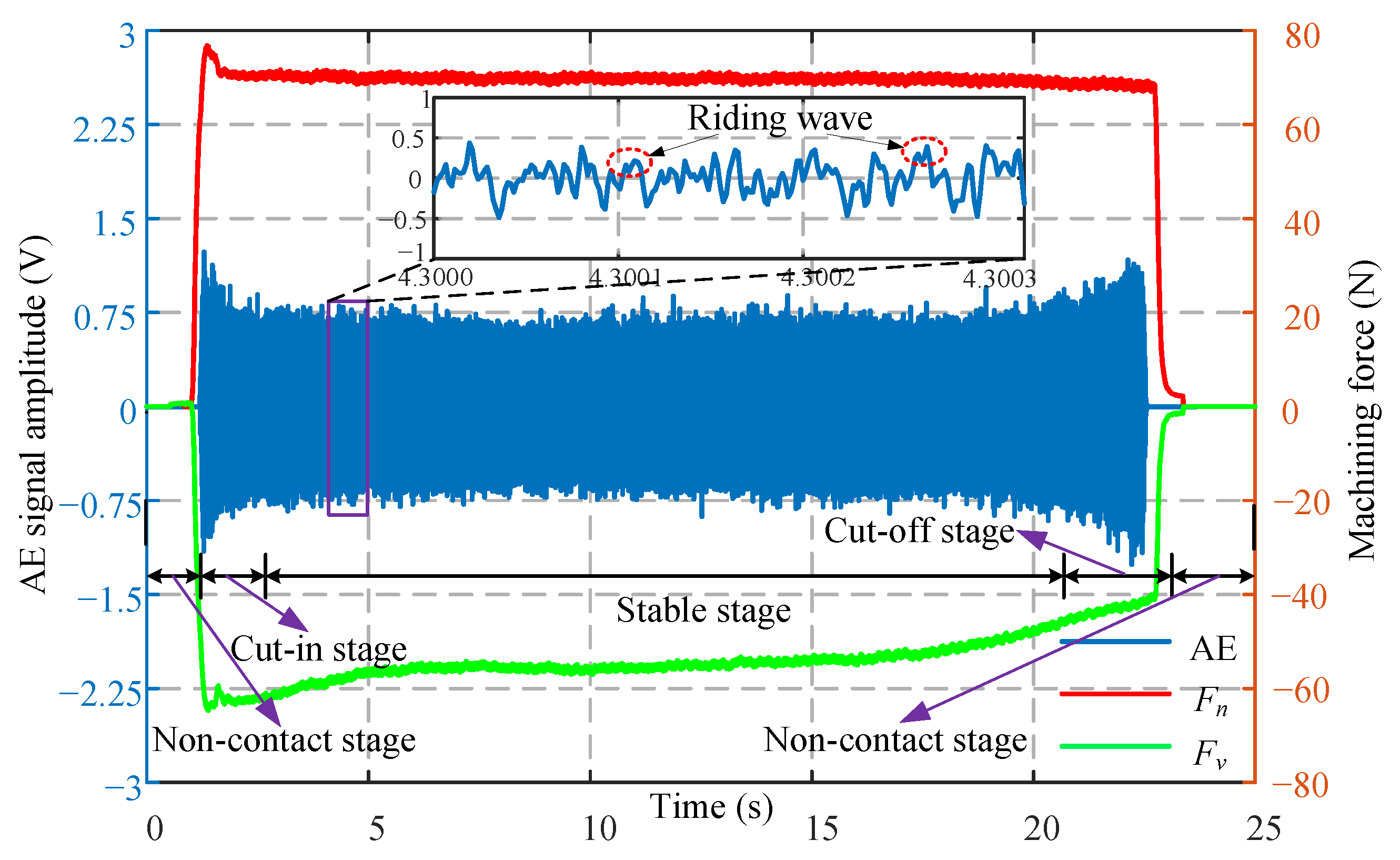
Figure 1 shows the actual collection of grinding force and AE signals in the robotic machining process, which demonstrates that the complete AE signal mainly includes four stages: non-contact stage, cut-in stage, stable stage, and cut-off stage. In the non-contact stage, the signal amplitude is small and primarily contributes to the background noise of the AE signal collection system, where the abrasive belt is not in touch with the machined material. In contrast, the signal amplitude fluctuates obviously during the cut-in and cut-off stages, which correlate to the beginning and leaving of the robotic belt grinding process, respectively. The continuous normal force causes steady signal amplitude variations in the stable phase. The local magnification image shows the local features of the AE signal, which exhibits irregular amplitude, variable period, the phenomenon of riding waves, and strong nonlinear and unsteady states.

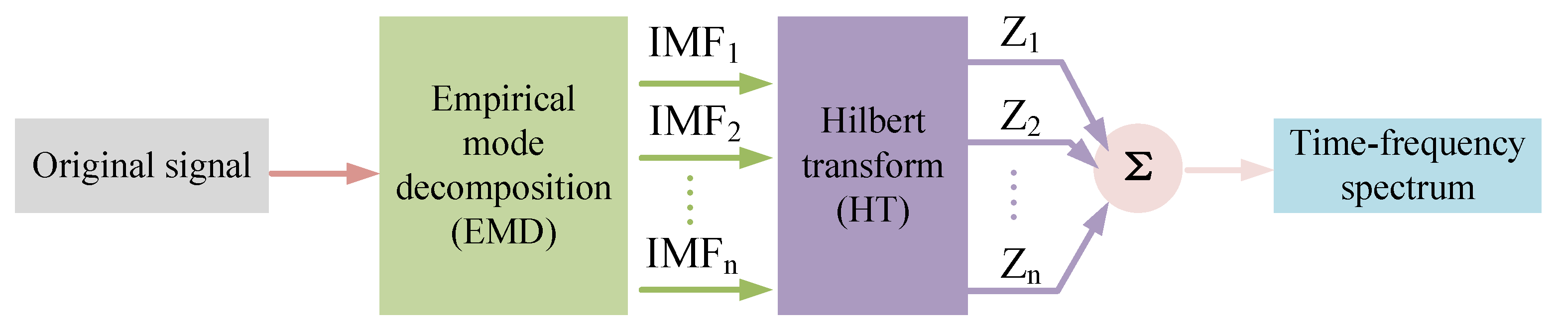
According to the analysis of AE signal characteristics, Hilbert–Huang transform (HHT) [20] is chosen as the time-frequency domain analysis method for AE signals in a robotic grinding system to reveal the robotic grinding mechanism for Ti-6Al-4V alloy workpieces. Figure 2 depicts the schematic of the HHT method, which is divided into empirical mode decomposition (EMD) and Hilbert transform (HT). Among these, the original signal is divided into a number of IMFs with physical significance that are decomposed from high to low frequency based on EMD.

Then, the Hilbert spectrum is selected to analyze each order of IMF components. The following is the definition of the Hilbert transform [23] for the signal $x\left(t\right)$:

$$H\left[x\left(t\right)\right]={\displaystyle \frac{1}{\pi }}·\mathrm{PV}{\int }_{-\infty }^{\infty }{\displaystyle \frac{x\left(\tau \right)}{\tau -t}}d\tau$$

(1)

where PV denotes the integral’s Cauchy principal value. The real domain signal $x\left(t\right)$ can then be converted into the complex domain signal $z\left(t\right)$ as follows:

$$z\left(t\right)=x\left(t\right)+j·H\left[x\right(t\left)\right]$$

(2)

The instantaneous amplitude and frequency of the signal $x\left(t\right)$ are as follows:

$$\left\{\begin{array}{c}a\left(t\right)=\sqrt{x^2\left(t\right)+H^2\left[x\left(t\right)\right]}\hfill \\ w\left(t\right)={\displaystyle \frac{d\left(\arctan \left(H\left[x\right(t\left)\right]/x\left(t\right)\right)\right)}{dt}}\hfill \end{array}\right.$$

(3)

The final original signal can thus be written as $X\left(t\right)$ in the complex domain by applying Equations (1)–(3) to each aforementioned order of ${\mathrm{IMF}}_i$ components [23]:

$$X\left(t\right)=\sum _{i=1}^n{a}_i\left(t\right)e^{j\int w_i\left(\tau \right)d\tau }$$

(4)

where $a_i\left(t\right)$ and $w_i\left(t\right)$ are functions of the amplitude and frequency of ${\mathrm{IMF}}_i$ components, respectively. The Hilbert spectrum of the original signal can be obtained:

$$H(w,t)=\mathrm{Re}\left(\sum _{i=1}^n{a}_i\left(t\right)e^{j\int w_i\left(\tau \right)d\tau }\right)$$

(5)

Among these, Re is the real component of the original signal $X\left(t\right)$. $H(w,t)$ is a comprehensive time–frequency–energy joint spectrum that can reflect the frequency changes over time but also track changes in the energy of the signal over frequency and time. Then, the Hilbert marginal spectrum [23] can be:

$$h\left(w\right)={\int }_0^{T}H(w,t)dt$$

(6)

where T is the signal’s duration in time and $h\left(w\right)$ the marginal spectrum.

2.2. Improved CCEEMD Algorithm of AE Signal in Robotic Machining System

Due to its excellent data adaptability, the Hilbert–Huang transform (HHT), which has no fixed basis function and does not require a choice of basis function in advance, is excellent for assessing AE signals. The EMD algorithm is required for the Hilbert–Huang transform to run smoothly, which affects the quality of signal analysis results. Academics have focused on the EMD algorithm [24], and an improved AE signal processing method is proposed to acquire the efficient time-frequency domain information during the robotic grinding process of workpieces.

2.2.1. EMD Algorithm and Its Derivatives of AE Signal

Empirical mode decomposition (EMD) is an adaptive data analysis method proposed by Huang et al. [23] in 1998, which has significant advantages in the analysis of nonlinear unsteady signals, and its core idea is to decompose the signal $x\left(t\right)$ into a number of intrinsic mode functions (IMF) and a trend term:

$$x\left(t\right)=\sum _{i=1}^n{\mathrm{IMF}}_i\left(t\right)+r_n\left(t\right)$$

(7)

where ${\mathrm{IMF}}_i\left(t\right)$ and $r_n\left(t\right)$ are the natural mode function and overall trend of the signal, respectively.

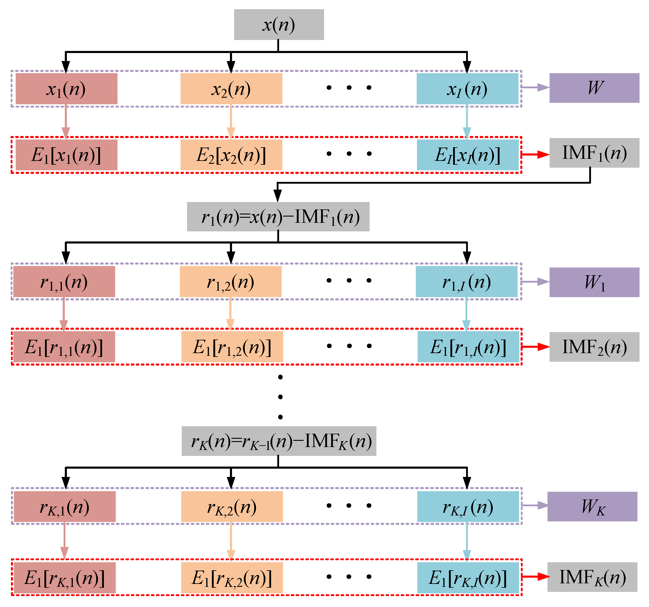
Figure 3 is used to explain why CEEMDAN is introduced before CCEEMD. Specifically, it visualizes the adaptive-noise decomposition sequence and residual-update path, which directly correspond to the modal-aliasing suppression logic described in the text. The distribution of the signal’s extremum points serves as the foundation for the highly adaptable decomposition outputs of the EMD algorithm, which only employs local extremum drives to finish signal selection. However, the system still suffers from mode aliasing because there are numerous riding waves in the signal (as depicted in Figure 1), which results in local intermittency of the signal and causes serious mode aliasing in its time-frequency distribution as well as blurring or losing of the physical meaning of its single IMF, seriously affecting the outcomes of signal analysis [25]. Therefore, modal aliasing must be suppressed and eliminated to accurately analyze AE signals in the robotic grinding system.

Then, an adaptive Complete Ensemble Empirical Mode Decomposition (CEEMDAN) method is proposed to address the above issue [26], as shown in Figure 3. The set W is considered as a whole, and the decomposition of its components is synchronized. Next, a particular limited white noise is added to the decomposition of each layer, which could solve the first-order modal function of all noise signals and receive the intrinsic mode function of the associated level of the signal $x\left(t\right)$. Finally, the residual $r\left(t\right)$ is calculated, and the procedure is repeated until the stopping condition is satisfied [23]. Therefore, the sequential execution approach of CEEMDAN algorithm effectively addresses the issues of reconstruction error, modal aliasing suppression and decomposition completeness.

2.2.2. Improved CCEEMD Algorithm of AE Signal

Although the CEEMDAN method outperforms the EMD algorithm, it still exhibits residual noise and “false” patterns [27]. The primary challenge is to reduce the residual noise in the IMF of the AE signal while maintaining the algorithm’s real-time efficiency and decomposition completeness. The Complementary Ensemble Empirical Mode Decomposition (CEEMD) method was proposed by Yeh et al. [28], and the set W could be divided into two parts by adding positive and negative pairs of auxiliary white noise to the original signal (the positive white noise set $W_{+}$ and the negative noise set $W_{-}$):

$$\left\{\begin{array}{c}{W}_{+}=\left\{x_i\left(n\right)\mid x_i\left(n\right)=x\left(n\right)+\xi ·w_i^{+}\left(n\right),i=1,2,\dots ,I\right\}\hfill \\ W_{-}=\left\{x_i\left(n\right)\mid x_i\left(n\right)=x\left(n\right)+\xi ·w_i^{-}\left(n\right),i=1,2,\dots ,I\right\}\hfill \end{array}\right.$$

(8)

where $\xi$ denotes the amplitude scaling factor of the introduced auxiliary white noise, which controls noise intensity to achieve an optimal trade-off between denoising effectiveness and signal fidelity. The added white noise in the set $W_{+}$ and $W_{-}$ meets the condition: $w_i^{-}\left(n\right)=-w_i^{+}\left(n\right)$, and it can be

$$E_j\left[w_i^{-}\left(n\right)\right]=E_j\left[-w_i^{+}\left(n\right)\right]=-E_j\left[w_i^{+}\left(n\right)\right]$$

(9)

It is demonstrated that the residual noise can be negated as much as possible throughout the signal IMF solution process and that the white noise with positive and negative pairs has IMF components that are diametrically opposed to one another. The CEEMD method outperforms the EMD algorithm in terms of decomposition efficiency and reconstruction error, but it suffers from alignment problems and a lack of decomposition completeness.

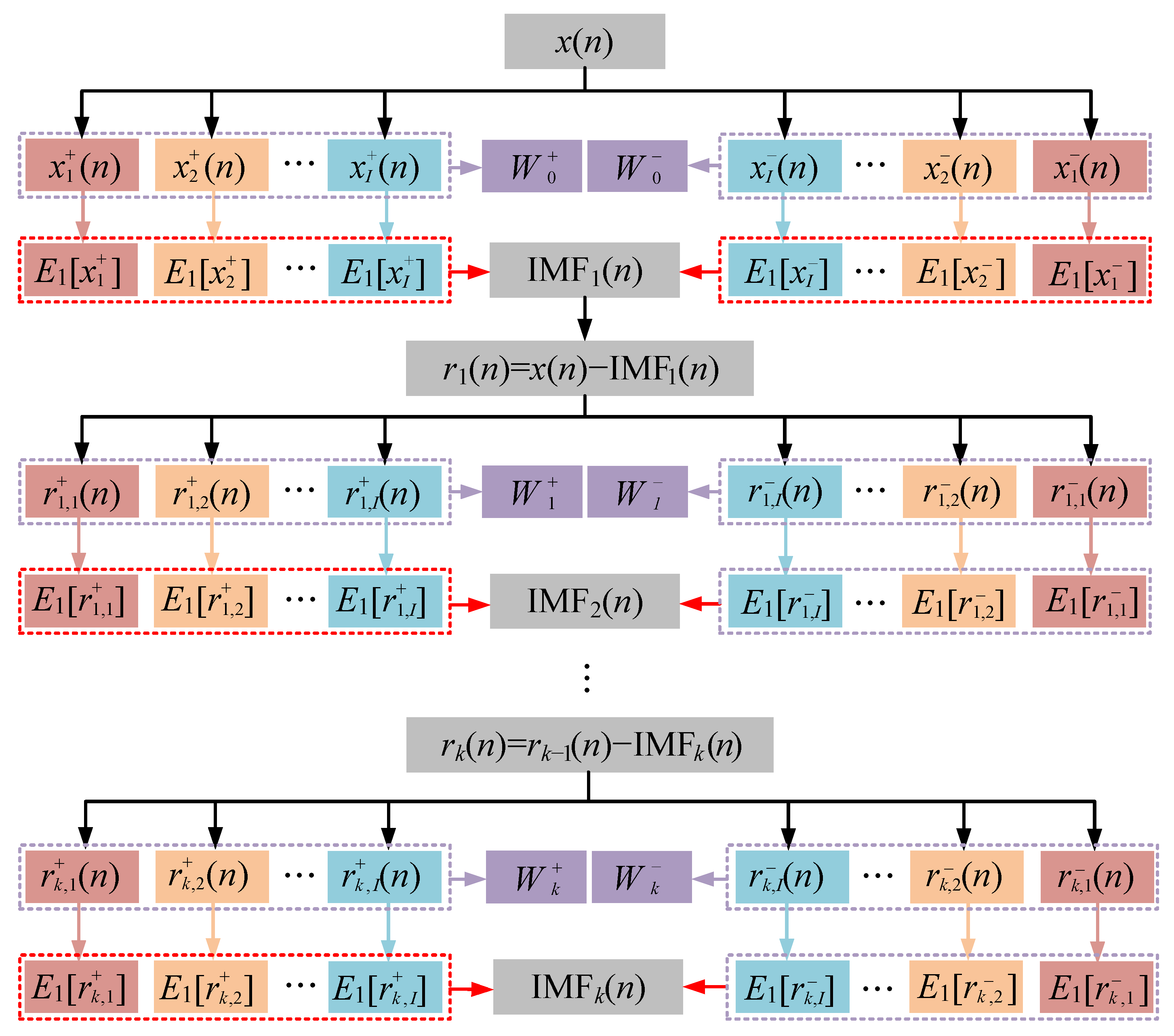
Therefore, an improved Completely Complementary Ensemble Empirical Mode Decomposition (CCEEMD) strategy is introduced to address the aforementioned shortcomings by merging the advantages of the CEEMD with the CEEMDAN algorithm. The initial signal is then defined as being $x\left(n\right)$, the corresponding noise sets are $W_{+}$ and $W_{-}$, and the natural mode functions and residuals of order k (k = 0, 1, 2 …, K) are then denoted as ${\mathrm{IMF}}_k\left(n\right)$ and $r_k\left(n\right)$, respectively. The detailed steps of the algorithm are as follows, and its schematic is shown in Figure 4.

(1)

Initialization: $r_0\left(n\right)=x\left(n\right)$, and k = 0;

(2)

Construct the kth-order noise-containing sets $W_k^{+}$ and $W_k^{-}$, then, a series of finite variance noise sequences $E_k\left[w_i\left(n\right)\right]$ should be added to the kth-order residual $r_k\left(n\right)$ using the following formula, where $w_i\left(n\right)$ (i = 1, 2, …, I) is the white noise that follows the $N(0,1)$ distribution:

$$\left[\begin{array}{c}{r}_k^{+}\left(n\right)\\ r_k^{-}\left(n\right)\end{array}\right]=\left[\begin{array}{cc}1& 1\\ 1& -1\end{array}\right]\left[\begin{array}{c}{r}_k\left(n\right)\\ {\xi }_k·E_k\left[w_i\left(n\right)\right]\end{array}\right]$$

(10)

(3)

Solve the $(k+1)$th order natural mode function using the following equation:

$${\mathrm{IMF}}_{k+1}\left(n\right)={\displaystyle \frac{1}{2I}}·\left(\sum _{i=1}^I{E}_1\left[r_k^{+}\left(n\right)\right]+\sum _{i=1}^I{E}_1\left[r_k^{-}\left(n\right)\right]\right)$$

(11)

(4)

Calculate the $(k+1)$th residual: $r_{k+1}\left(n\right)=r_k\left(n\right)-{\mathrm{IMF}}_{k+1}\left(n\right)$;

(5)

Determine whether residual $r_{k+1}\left(n\right)$ meets the stopping criterion; if not, $k=k+1$, then continue execution at Step 2; if so, the algorithm stops and the final residual is:

$$R\left(n\right)=x\left(n\right)-\sum _{k=1}^K{\mathrm{IMF}}_k\left(n\right)$$

(12)

where K represents the final number of signal decomposition layers and the decomposition of signal $x\left(n\right)$ is accurate.

Figure 4 summarizes the full CCEEMD workflow from initialization, complementary-noise injection, IMF extraction, and residual iteration to stopping criteria. The step-by-step equations are retained because each equation corresponds to one required operation in the implemented algorithm. For computational-cost clarification, if the signal length is N, decomposition layers are K, and ensemble size is I, the dominant complexity of the proposed decomposition is $\mathcal{O}\left(IKN\right)$. In our implementation, the parameter ranges were selected as $\xi \in [0.1,0.3]$ and $I\in \{50,100,200\}$ through pilot tests balancing decomposition stability and runtime. The final setting ($\xi =0.2$, $I=100$) provided stable IMF separation with acceptable computational cost in the robotic grinding dataset.

2.3. AE Signal Denoising Method Based on Monte Carlo

There is a strong background noise present in the actual gathered AE signals during the robotic machining system because of the coupled vibration between the robot and the grinding machine measuring equipment and the influence of the environmental noise interference. Therefore, a noise removal algorithm based on statistical hypothesis testing is introduced to obtain the time-frequency statistical characteristics of the IMF through the results of a Monte Carlo experiment, and the components that match the IMF background noise characteristics would then be removed to achieve denoising.

The noise in the normal robotic machining state is derived from several aspects: the friction between the abrasive belt and workpiece; the coupled vibration of the robotic machining system caused by the local intermittent and unstable grinding and abrasive grain wear; and the background noise of the AE sensor and signal acquisition system. Therefore, the actual collected AE signal $x\left(t\right)$ is the fusion of the effective AE signal $s\left(t\right)$ and noise signal $n\left(t\right)$:

$$x\left(t\right)=s\left(t\right)+n\left(t\right)$$

(13)

If the noise signal $n\left(t\right)$ is independent and identically distributed Gaussian white noise, its spectral distribution characteristic is reflected in the fact that the power spectral density is constant, which is different from the relatively concentrated spectral distribution of useful signals. Using computer numerical simulation technology, Wu et al. [25] conducted several experimental research studies on the statistical characteristics of intrinsic mode functions (IMFs) produced by white noise decomposed using the EMD algorithm. Their key findings are as follows: For white noise with standard uniform or Gaussian distribution, the energy density $E_i$ of ${\mathrm{IMF}}_i$ ($i=1,2,\dots ,n$) and its associated average period $T_i$ satisfy the following relationship [29]:

In this study, the Gaussian white-noise assumption is applied to the background component after removing effective cutting intervals and normalizing stationary idle/no-load segments. The assumption is used as a statistical approximation for denoising decision-making, and the confidence-bound validation supports its applicability for the present AE acquisition conditions.

$$ln{E}_i+ln{T}_i=0$$

(14)

It shows that the product of the energy density $E_i$ and its corresponding average period $T_i$ is a constant, and the energy density $E_i$ of ${\mathrm{IMF}}_i$ is defined as the mean square sum of the ith $\mathrm{IMF}$, then:

$$E_i={\displaystyle \frac{1}{N}}·\sum _{j=1}^N{\mathrm{IMF}}_i^2\left(j\right)$$

(15)

N is the data amount of the ${\mathrm{IMF}}_i$, the average period $T_i$ is defined as the number of data points between adjacent maximum points in ${\mathrm{IMF}}_i$, and the maximum number ${\mathrm{IMF}}_i$ is set as $N_{max}$, then:

$$T_i={\displaystyle \frac{N}{N_{max}}}$$

(16)

The experimental findings demonstrate that the amplitudes of each order of the IMF components produced by EMD decomposition of normalized white noise follow a normal distribution. Therefore, the energy density of each order IMF component follows the chi-square distribution, and the boundary distribution equation of energy density $E_i$ is:

$$\ln E_i=-\ln T_i\pm k·\sqrt{{\displaystyle \frac{2}{N}}}·e^{\ln T_i/2}$$

(17)

where “+” and “−” represent the upper and lower boundaries of the distribution of logarithmic energy density $E_i$, respectively, and k is related to the confidence level, which is approximately equal to the quantile of the corresponding standard normal distribution at a certain confidence level.

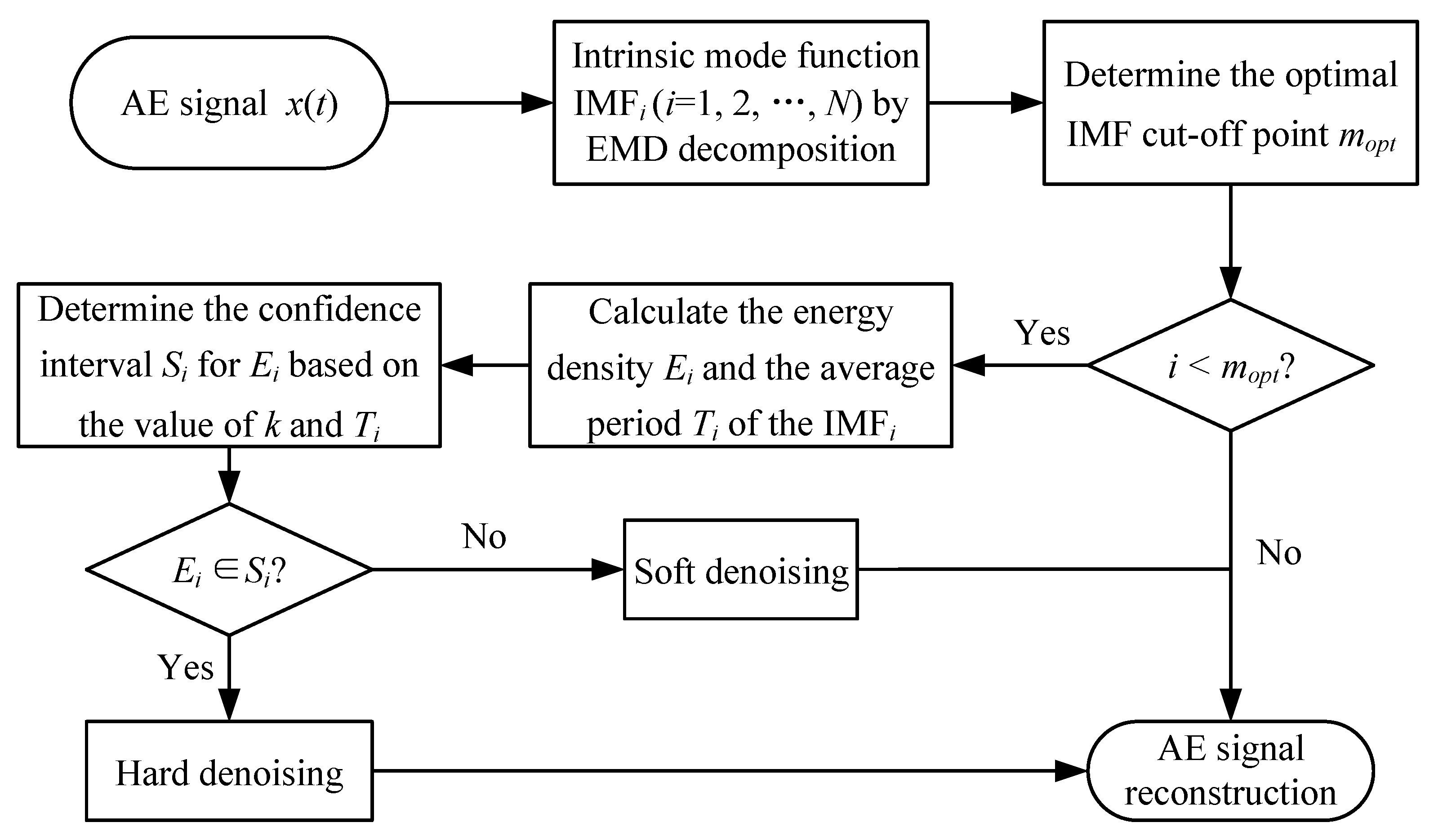
The hypothesis-testing decision rule is implemented as follows: $H_0$ indicates noise-dominant IMF components (inside the confidence bounds) and $H_1$ indicates informative IMF components (outside the confidence bounds). At 99% confidence ($k=2.34$), components satisfying Equation (18) are treated by hard denoising, while components satisfying Equations (19) or (20) are preserved and processed by soft thresholding. For unknown noise signals, the normalized signal by the EMD decomposition is the sum of a series of narrow band IMF components. If the unknown noise is assumed as white noise, the characteristics of each IMF component can be determined by computing the energy density and the average cycle of each IMF component. If they meet Equation (14), the IMF components are white noise; if not, the more they deviate from the line, the more statistically significant information they contain, and the less likely they are to be noise. The Monte Carlo verification method is used to investigate the relationship between energy density $E_i$ of ${\mathrm{IMF}}_i$ component and average period $T_i$.

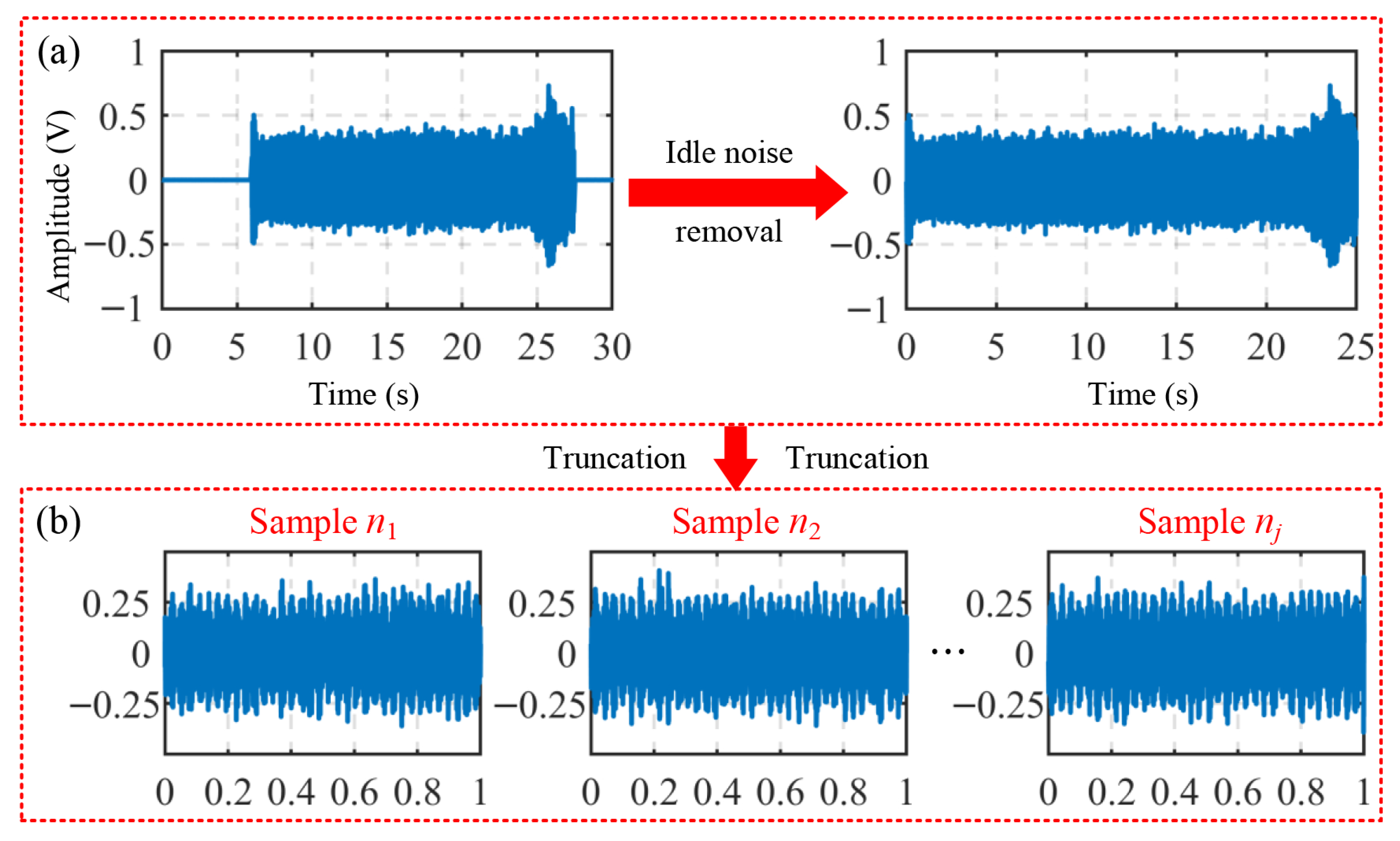
To optimize AE signal acquisition, the amplitude of the effective signal $s\left(t\right)$ should be minimized such that the measured raw signal $x\left(t\right)$ approximates the background noise level $n\left(t\right)$. This condition can be achieved by suppressing plastic deformation of the material during the measurement process. As a result, the serious wear of abrasive belts is used in the robotic grinding experiments to reduce or avoid producing as much material removal as possible. The background noise is truncated to obtain the noise signal sample $n_j$ (j = 1, 2, 3, …, 3000). The method of intercepting a sample signal is shown in Figure 5, and 3000 sample signals are ultimately acquired. Each sample signal $n_j$ was normalized according to the Z-score standardization method:

$$n_j^{\ast }={\displaystyle \frac{n_j-{\mu }_j}{{\sigma }_j}}$$

(18)

where ${\mu }_j$ and ${\sigma }_j$ are the mean and standard deviation of the sample signal $n_j$, respectively.

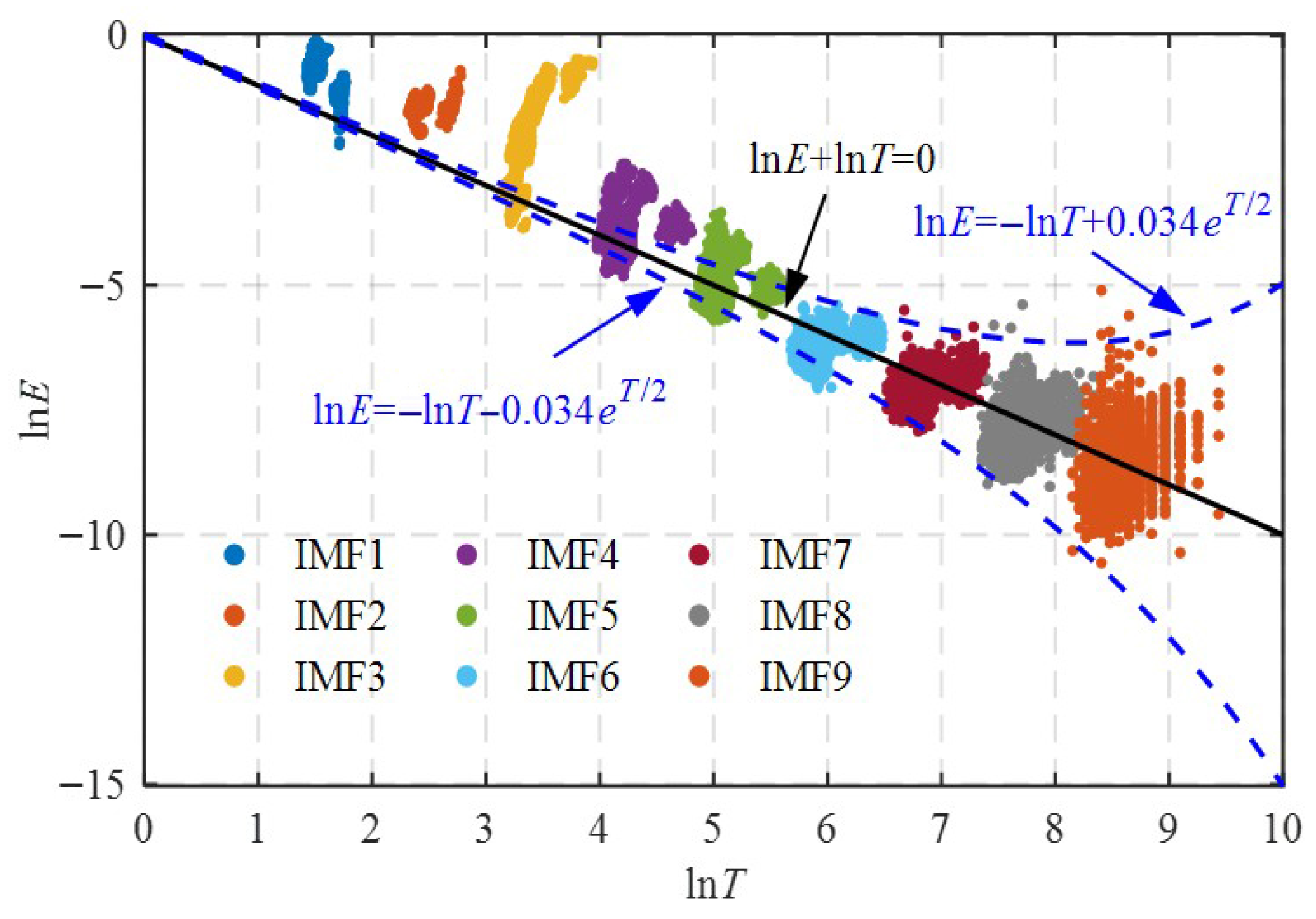
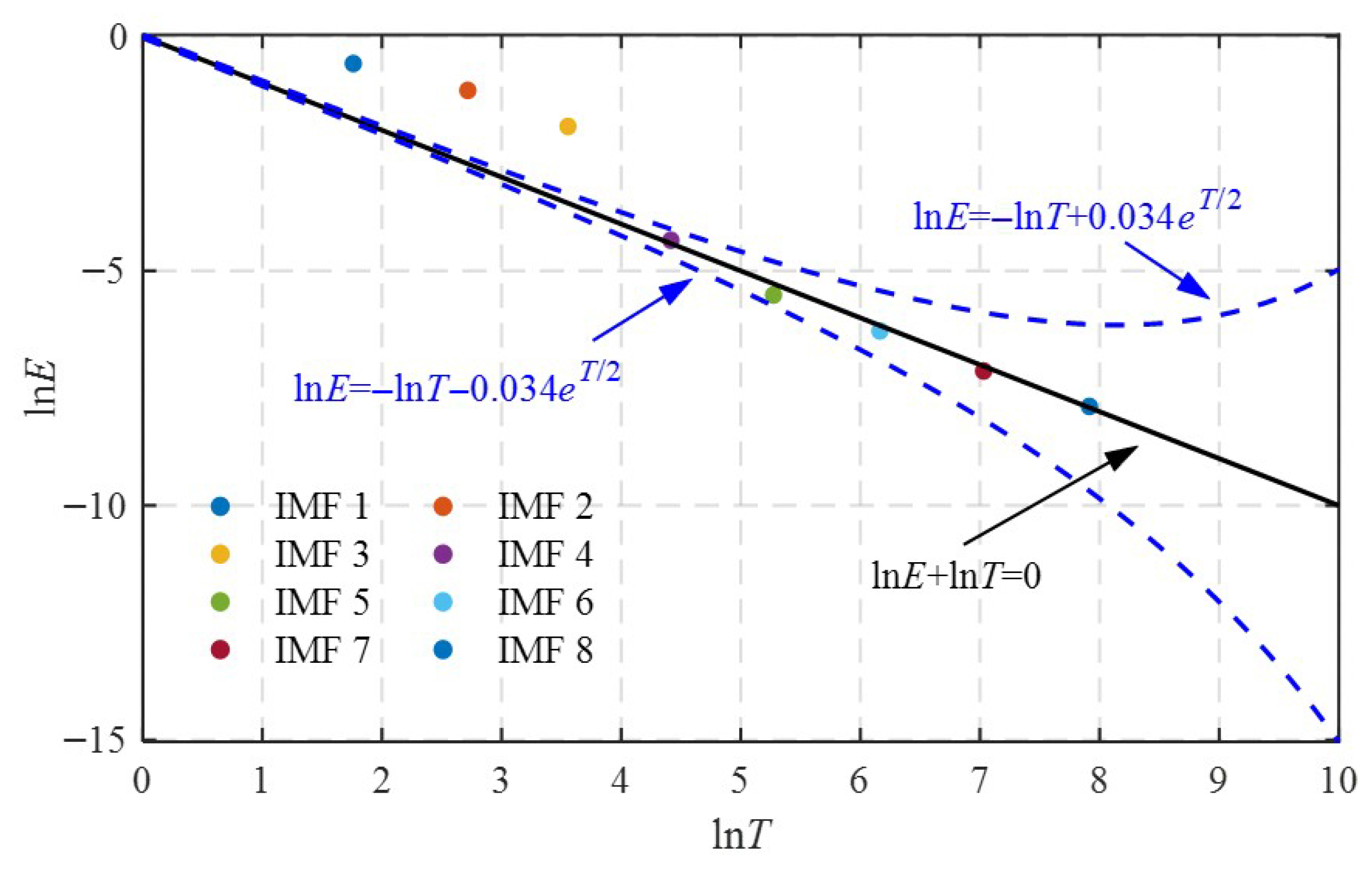
Through the Monte Carlo method, 3000 repeated samplings of noise signals were performed along with EMD. Following Equations (15) and (16), the energy density $E_i$ and mean period $T_i$ of each IMF component were computed and statistically analyzed to establish a benchmark statistical model for white noise. As illustrated in Figure 6, the logarithmic distributions of energy density $E_i$ and mean period $T_i$ were analyzed for ${\mathrm{IMF}}_i$ components across all 3000 noise samples. Statistical analysis at the 99% confidence level (k = 2.34) demonstrates strong agreement between the empirical distributions and the theoretical formulations presented in Equations (14) and (17). This analytical evidence confirms the equivalence in statistical properties between the white noise generated during robotic belt grinding processes and the ambient background noise. Certain points are distributed outside the boundary curve when specific parameter combinations are used, indicating that part of the gathered background noise includes some valuable information.

2.4. AE Signal Denoising Algorithm Based on Noise Statistical Characteristics

Based on the study above, the background noise in the robotic belt grinding process is defined as white noise, and the energy density and average period of its IMF satisfy Equations (14) and (17). Therefore, the relationship between energy density E and the average period T of the IMF component of the AE signal can be used to validate whether it is the background noise component; then the IMF component corresponding to noise can be removed to achieve the purpose of denoising in the signal reconstruction.

Using Equations (15) and (16), the energy density $E_i$ and average period $T_i$ can be solved for the original AE signal $x\left(t\right)$ after being normalized and decomposed using EMD to extract each component ${\mathrm{IMF}}_i$ (i = 1, 2, …, M), if $E_i$ and $T_i$ meets:

$$-\ln T_i-k·\sqrt{{\displaystyle \frac{2}{N}}}·e^{\ln T_i/2}\le \ln E_i\le -\ln T_i+k·\sqrt{{\displaystyle \frac{2}{N}}}·e^{\ln T_i/2}$$

(19)

It implies that ${\mathrm{IMF}}_i$ is inside the upper and lower boundary curves and can be considered as pure noise, then all of the amplitude can be ${\mathrm{IMF}}_i\left(j\right)$ = 0 by using the hard denoising method, where j = 1, 2, 3, …, N. On the other hand, if $E_i$ and $T_i$ meets:

$$\ln E_i>-\ln T_i+k·\sqrt{{\displaystyle \frac{2}{N}}}·e^{\ln T_i/2}$$

(20)

or

$$\ln E_i<-\ln T_i-k·\sqrt{{\displaystyle \frac{2}{N}}}·e^{\ln T_i/2},$$

(21)

this indicates that ${\mathrm{IMF}}_i$ is spread outside the upper and lower border curves and is primarily made up of effective signals. Due to the fact that white noise has the property of uniform distribution over the entire frequency range and the associated noise amplitude is very low, the IMF component fulfilling Equations (19) or (20) still contains noise. Therefore, the soft denoising method is used:

$${\mathrm{IMF}}_i{\left(j\right)}^{\ast }=\left\{\begin{array}{cc}\mathrm{sgn}\left({\mathrm{IMF}}_i\left(j\right)\right)·\left(|{\mathrm{IMF}}_i\left(j\right)|-{\chi }_i\right),\hfill & |{\mathrm{IMF}}_i\left(j\right)|>{\chi }_i;\hfill \\ 0,\hfill & |{\mathrm{IMF}}_i\left(j\right)|\le {\chi }_i.\hfill \end{array}\right.$$

(22)

where $\mathrm{sgn}(\ast )$ is the sign function, ${\chi }_i$ is the threshold value of ith $\mathrm{IMF}$ component, and ${\chi }_i=3{\sigma }_i$ in accordance with the “3$\sigma$” principle, which is conformed to the distribution rule of the coefficient of background noise $\mathrm{IMF}$ component; among the ${\sigma }_i$ is the standard deviation of ${\mathrm{IMF}}_i$.

The execution times of the above denoising algorithm are related to the number of decomposition layers M of the EMD algorithm. For signals with drastic changes in local features and plenty of data points, the number of decomposition layers is usually $M\ge 10$. Denoising the $\mathrm{IMF}$ components on every layer M will require a long period; it is required to further confirm the primary distribution layers of noisy energy to improve the effectiveness of the denoising algorithm. Therefore, $C\left(m\right)$ is defined as the energy of the m-order $\mathrm{IMF}$ and its proportion of the total energy.

$$C\left(m\right)=\sum _{i=1}^m{E}_i/\sum E_i$$

(23)

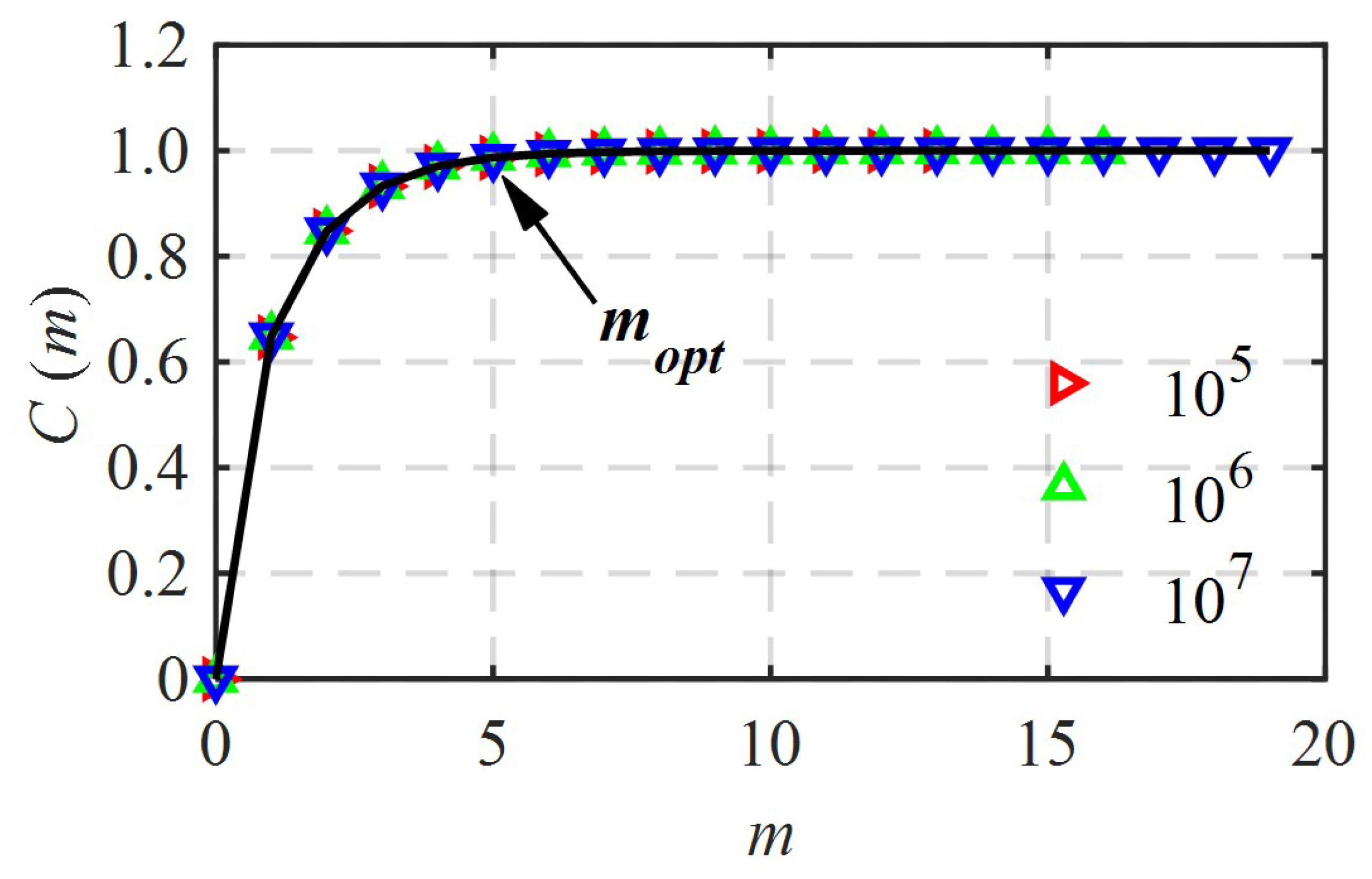
The larger $C\left(m\right)$ is, the more energy the noise distributes in the first m-order, and the smaller its influence on the later m-order. Figure 7 shows the variation of the specific gravity $C\left(m\right)$ with the cumulative order m when the number of white noise data points are ${10}^5$, ${10}^6$ and ${10}^7$, respectively. It can be seen that the variation tendency of three curves is nearly similar, and an optimal $\mathrm{IMF}$ cut-off point $m_{opt}$ exists with a corresponding energy proportion $C\left(m_{opt}\right)=98.68\%$. The energy proportion $C\left(m\right)$ changes extremely slowly after the order of the cut-off point $m_{opt}$, indicating that the energy of the subsequent noise $\mathrm{IMF}$ component is very low and less than 2%. Therefore, the optimal $\mathrm{IMF}$ cut-off point $m_{opt}$ is defined as the order corresponding to the specific gravity $C\left(m\right)$ exceeding 98% for the first time, and the signal denoising algorithm is performed for the $\mathrm{IMF}$ component with order $i\le m_{opt}$, while the impact of noise can be disregarded for the $\mathrm{IMF}$ with order $i>m_{opt}$ and the remaining trend term.

As a result, Figure 8 illustrates the specific steps of the AE signal denoising technique based on the statistical characteristics of background noise in the robotic grinding process, which are primarily divided into soft denoising and hard denoising. Figure 8 is explained as an executable denoising pipeline: IMF decomposition, energy-period feature extraction, confidence-bound decision, and hard/soft denoising reconstruction. This explicit mapping is added to improve the readability of the algorithm derivation.

3. Experimental Results and Discussions

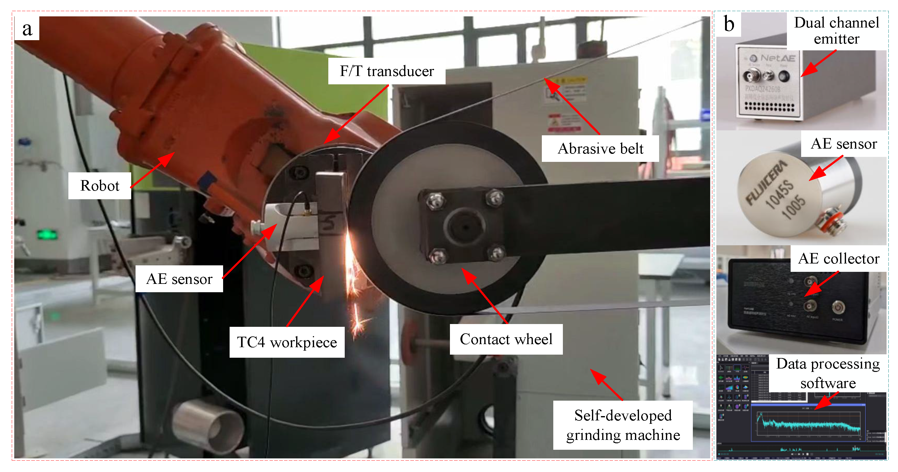
The robotic abrasive grinding system, depicted in Figure 9, is composed of a robot motion unit (ABB IRB4400, ABB Robotics, Zurich, Switzerland), a force control unit (ATI Omega 160, ATI Industrial Automation, Apex, NC, USA), a self-designed grinder machine with a 3M pyramid abrasive belt, and a Ti-6Al-4V alloy workpiece. While the AE signal sampling and processing system are composed of a dual-channel acoustic emitter, a 1045S wideband AE sensor, an AE signal collector and data processing software, the detailed parameter settings of the AE sensor are as follows: the sampling frequency, signal threshold, and pre-filtering energy are set as 1.25 MHz, 40 dB, and 50 kHz, respectively. The robot is an ABB IRB4400 (6-DOF) manipulator; the manufacturer-specified repeatability is ±0.07 mm.

3.1. Time-Frequency Analysis of AE Signal in Robotic Machining System

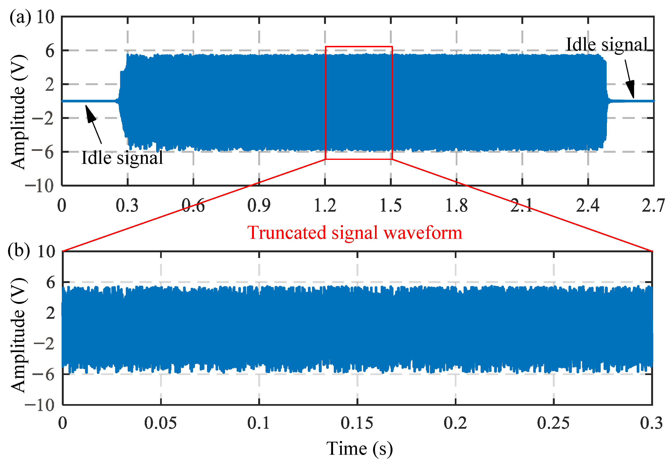
The AE information acquisition system includes the whole robotic belt grinding operation with idle information (about 500,000 data points), as illustrated in Figure 10a. Therefore, the collected AE signals are preprocessed to obtain the effective machining information.

It is revealed that the actual AE signal sampling time of the robotic belt grinding experiment is about 2 s (about 2.5 million data points), and the original signals should be truncated with the longest rotation time of the abrasive belt. Therefore, the truncation processing time of the AE signal is selected as 0.3 s; as shown in Figure 10b, the length of each section of the AE signal is controlled at 375,000 sampling points.

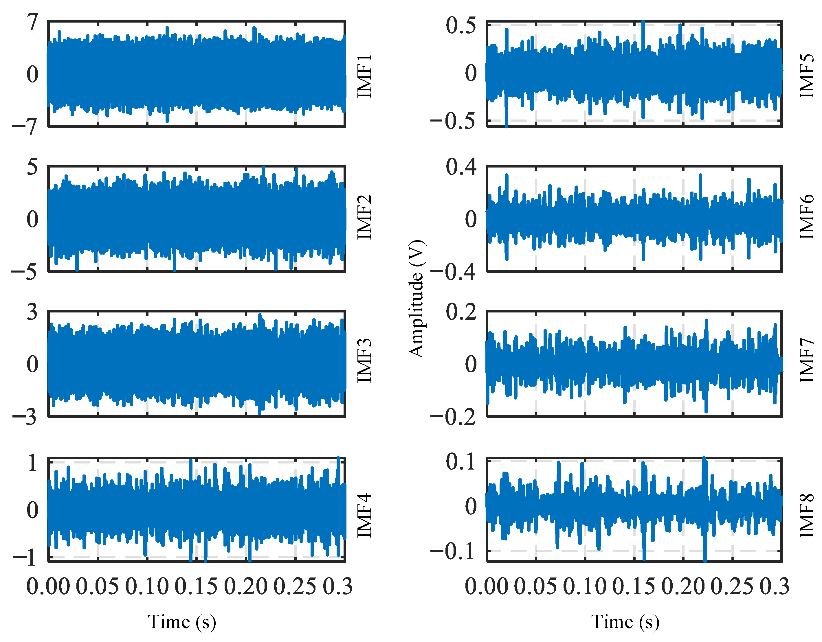
The CCEEMD method is an iterative decomposition process, and higher-order IMF components predominantly consist of negligible signal elements and residual noise, while the critical characteristic features of AE signals are primarily concentrated within the first eight IMF orders. Figure 11 is the first 8-order IMF components of the AE signal after the decomposition of the proposed CCEEMD algorithm during the robotic belt grinding system with processing parameters: normal force $F_n$ = 50 N, belt linear velocity $v_s$ = 16.75 m/s, robot feed rate $v_r$ = 5 mm/s, and contact wheel hardness $H_c$ = 30 HRC. It is demonstrated that each IMF component can reflect AE signals at different time scales. High-order IMF components typically correspond to long periods and low frequencies, while low-order IMF components correlate to short periods and high frequencies [20]. Meanwhile, the signal amplitude of each order IMF component is different, and as IMF component orders increase, the signal amplitude eventually declines.

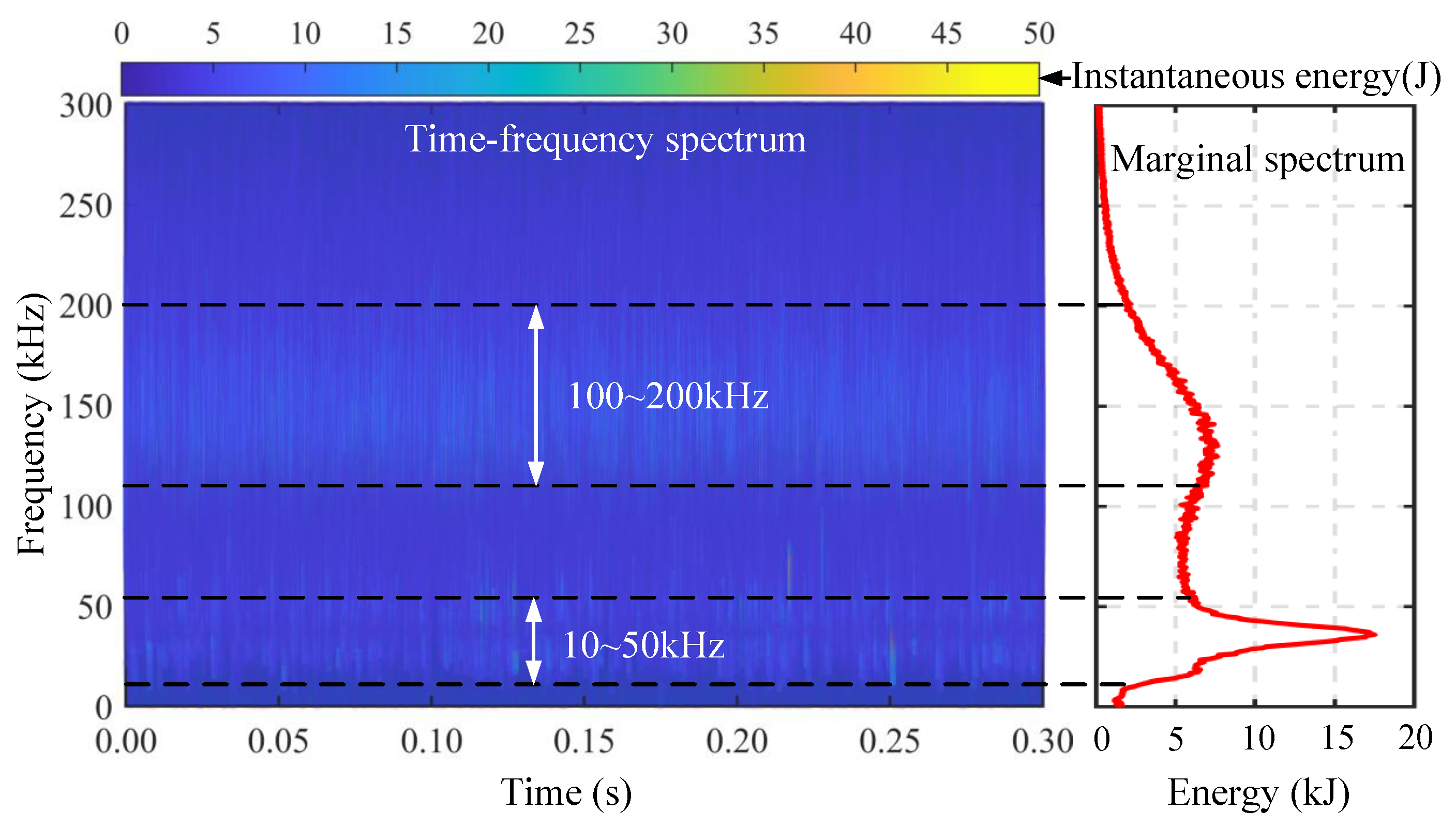
The Hilbert transform was applied to the IMF components obtained through CCEEMD decomposition to generate the time-frequency and marginal spectra of the AE signals, as shown in Figure 12, enabling detailed analysis of the frequency distribution characteristics of each IMF component. Our spectral analysis identified two distinct high-energy frequency bands at 10–50 kHz and 100–200 kHz. This finding contrasts with the results reported by Pandiyan et al. [10], who associated similar frequency bands with three distinct abrasive belt grinding phases: sliding and plowing phenomena occurring at 25–125 kHz and chip formation processes corresponding to 125–350 kHz.

AE signals are intrinsically linked to the plastic deformation of metallic materials, and a key distinction between sliding and plowing effects lies in their deformation mechanisms: sliding predominantly induces elastic deformation, whereas plowing leads to plastic deformation and subsequent chip formation. In contrast to the findings of Pandiyan et al. [10], our experimental results demonstrate that the 10–50 kHz free band exclusively corresponds to the sliding effect of abrasive grains, while the 100–200 kHz range is associated with the plowing and chip formation. Notably, their results demonstrate that the sliding stage occurs within a frequency range of 25–75 kHz, which aligns closely with our experimental observations. Furthermore, the high-frequency band in our study (100–200 kHz) is significantly narrower than the 125–325 kHz range reported by Chu et al. [30]. This variation can be primarily attributed to three key factors: the specific type of belt, inherent differences in material properties, and variations in experimental parameter settings.

Figure 13 presents the distribution of average period versus energy for the IMF components in logarithmic coordinates, which enables discrimination between signal and noise components. Quantitative analysis reveals that the first three IMF components lie distinctly outside the confidence interval for noise signals, while subsequent components fall within the noise-dominated region. These results confirm that only the initial three IMF components represent meaningful signal information, whereas the remaining components should be eliminated through the proposed AE signal denoising method.

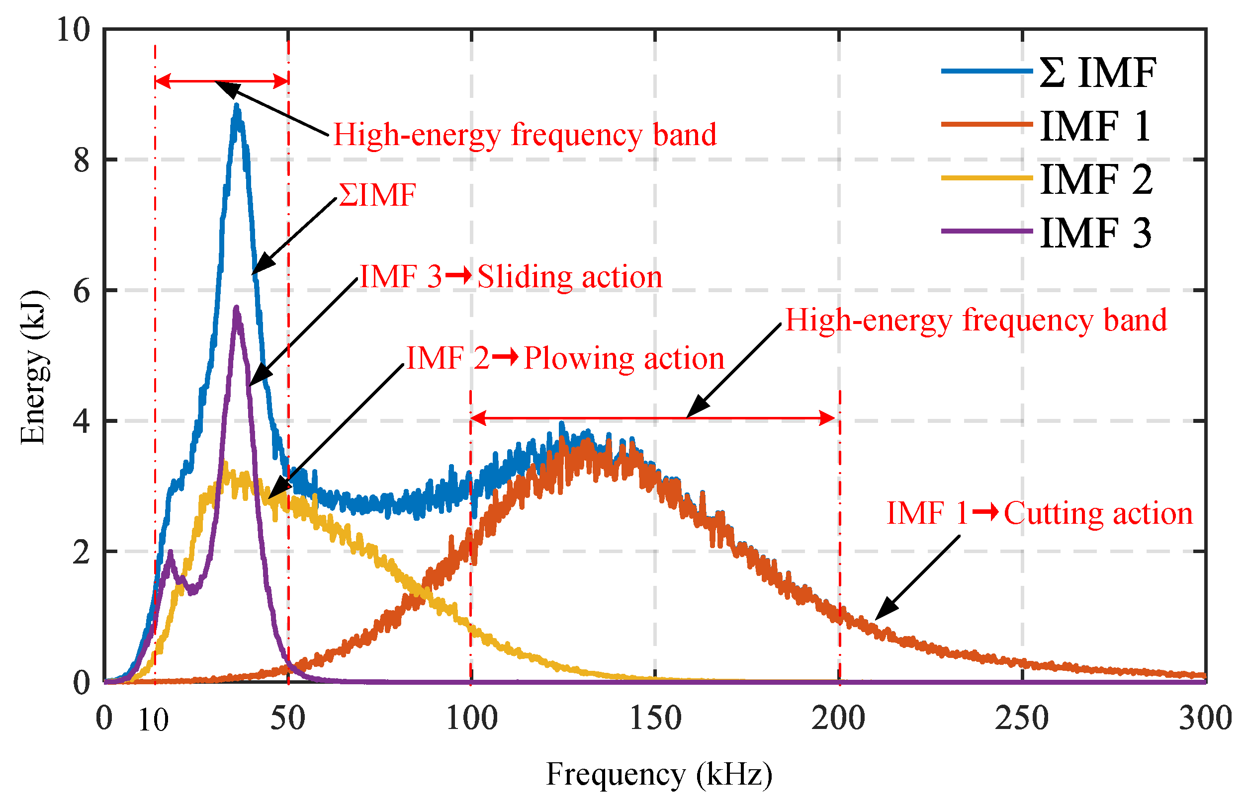
Whereas the non-noise IMF components are separately analyzed to characterise their frequency distribution range, Figure 14 presents the first three IMF components (IMF1–IMF3) along with their marginal spectra and combined spectrum. The analysis reveals that the composite marginal spectrum ($\Sigma$IMF) represents the algebraic superposition of individual IMF spectra, and each IMF component exhibits distinct dominant frequency ranges. Among the frequency distribution ranges, IMF1 and IMF3 components are compatible with the above-mentioned high-energy frequency band (100∼200 kHz and 10∼50 kHz), while the frequency range distribution of IMF2 falls between IMF1 and IMF3, and it is more inclined to the frequency band of IMF3. Therefore, these findings strongly support the correlation between the three IMF components and the fundamental stages of robotic abrasive belt processing (chip formation, plowing, and sliding, respectively). The observed frequency segregation provides quantitative evidence for energy partitioning during different material interaction phases.

3.2. Influence Analysis Between AE Signal and Grinding Mechanism

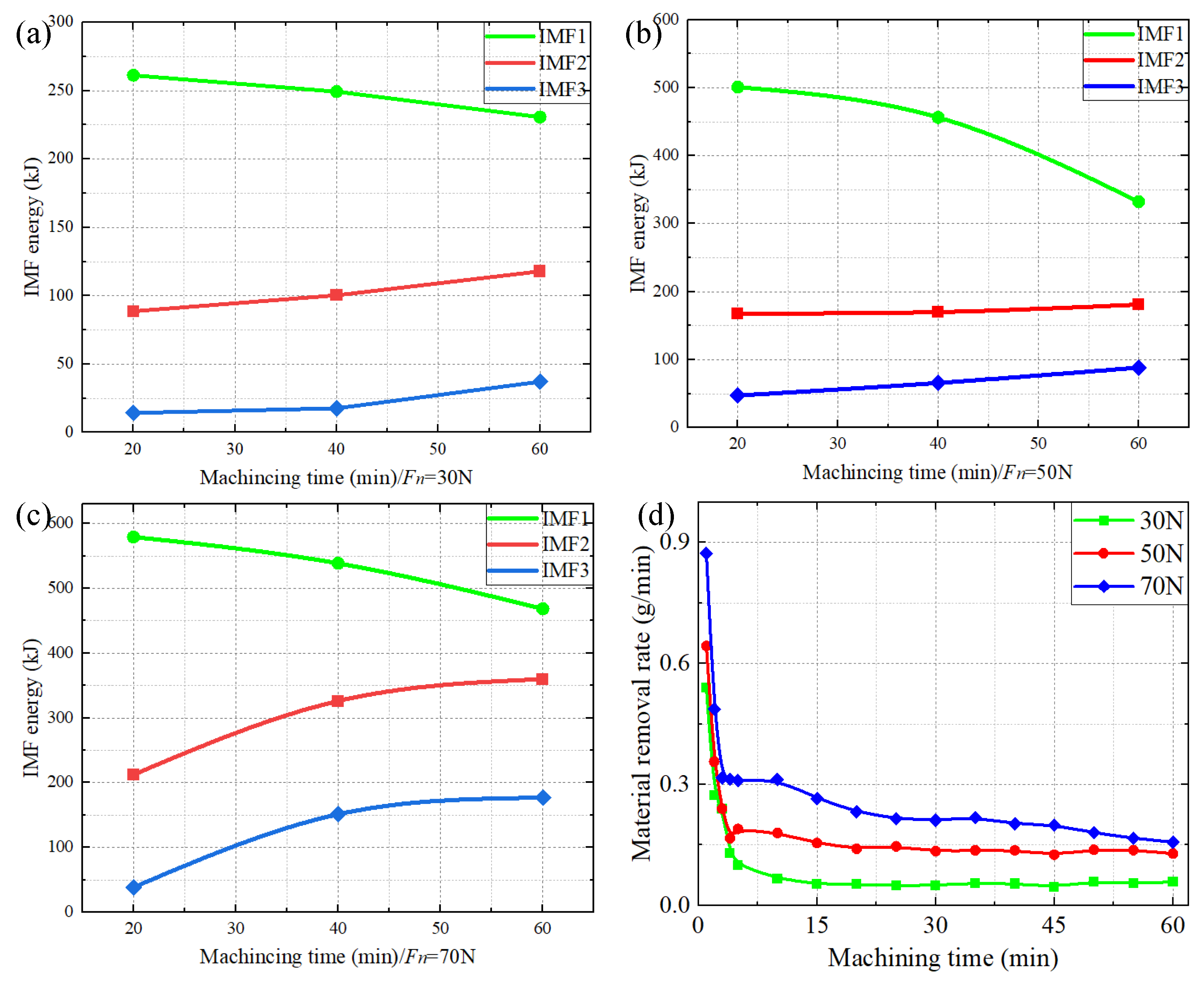
Figure 15 shows the changes of the IMF energy and material removal rate under various normal forces with the processing parameters: the belt linear velocity $v_s$ = 16.75 m/s, the robotic feed speed $v_r$ = 5 mm/s, the contact wheel hardness $H_c$ = 30 HRC, and the normal force $F_n$ = 30 N, 50 N, and 70 N, respectively. It is revealed that the energy of the IMF1 component gradually decreases with the machining time, while the energy of the IMF2 and IMF3 components both increase with the machining time under the same force, which is consistent with the change of cutting mechanism of the abrasive belt [10]. As the machining time increases, the cutting effect progressively weakens, while the plowing and sliding effect gradually strengthens, which is consistent with the changing trend of material removal [31]. Therefore, it can be demonstrated that the material removal rate will decrease with the machining time when all other factors remain constant, leading to an increase in the volume of material plastic deformation as well as the AE energy, as illustrated in Figure 15d. In conclusion, the three phases of abrasive belt cutting action are represented by the first three order components of the AE signal: IMF1 correlates to the cutting action, IMF2 to the plowing action, and IMF3 to the sliding action.

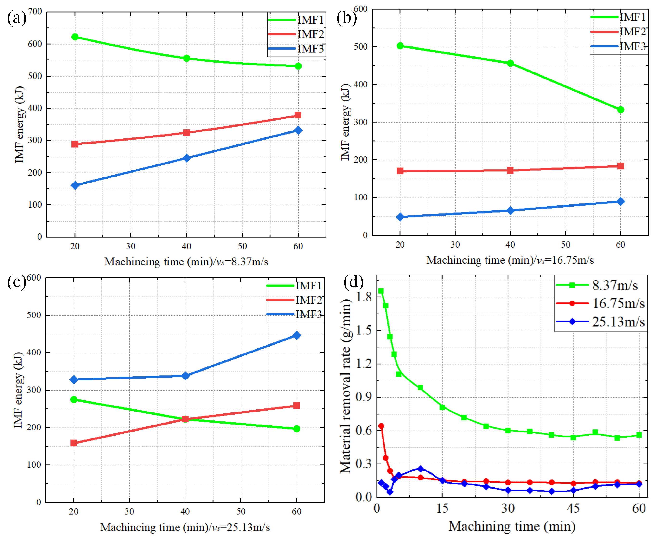
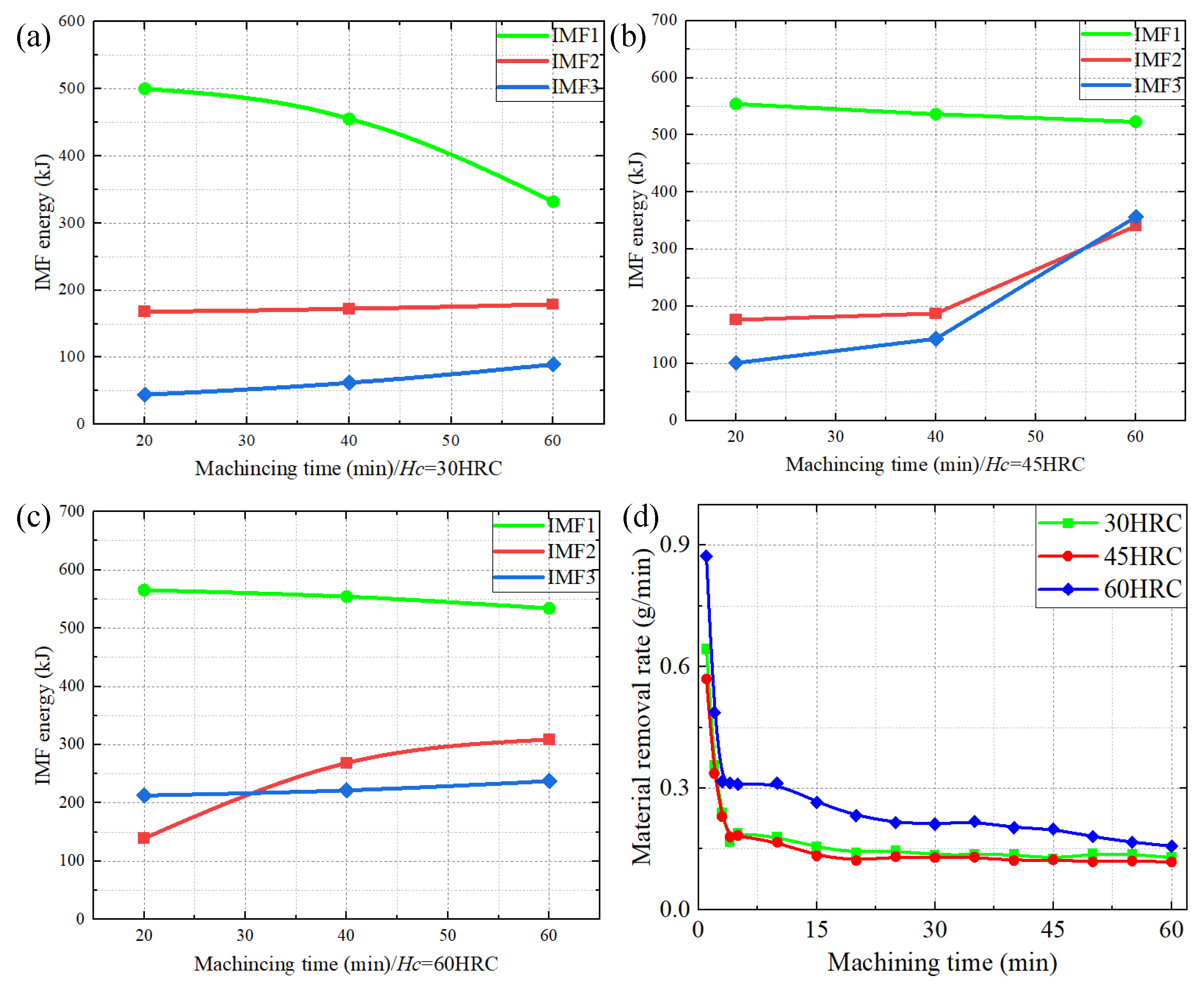
The robotic grinding mechanism is further revealed by analyzing the change trend of IMF energy and material removal rate at various linear velocities and contact wheel hardness, as shown in Figure 16 and Figure 17, respectively. It is illustrated in Figure 16a–c that the energy of IMF1 progressively declines with the machining time, while the energy of IMF2 and IMF3 both rise with the machining time under the same belt linear velocity, which is similar to the change trend of normal force analysis. However, the energy of the IMF3 component in Figure 16c is abnormally increased compared to other test findings. It is revealed that the IMF energy at a linear velocity of 8.37 m/s is significantly different from that of 25.13 m/s, indicating that the contact time between the abrasive grains and the workpiece is shortened with the increase of the belt linear velocity under certain conditions [30], resulting in the reduction of material removal rate, as illustrated in Figure 16d. In other words, the sliding and plowing effect of the robotic grinding process is relatively enhanced, while the chip-forming effect is relatively diminished.

The energy variation curves of the first three-order IMF components of the AE signal under varying contact wheel hardness in the robotic belt grinding process are shown in Figure 17a–c. It demonstrates that the energy variations in IMF1, IMF2 and IMF3 components are comparable to the trend in energy variation in normal force and belt linear velocity analysis. Additionally, the test results revealed that the energy of IMF1 gradually increases with contact wheel hardness and that there is a significant difference between the medium hard contact wheel ($H_c$ = 10–35 HRC) and the soft contact wheel ($H_c$ = 35–60 HRC). As contact wheel hardness increases, the abrasive cutting effect and IMF1 energy are enhanced [32], as illustrated in Figure 17d. However, the robotic soft processing becomes hard processing when contact wheel hardness reaches a certain point, deviating from the robotic flexible processing nature and increasing material removal at the expense of the workpiece’s surface quality [33].

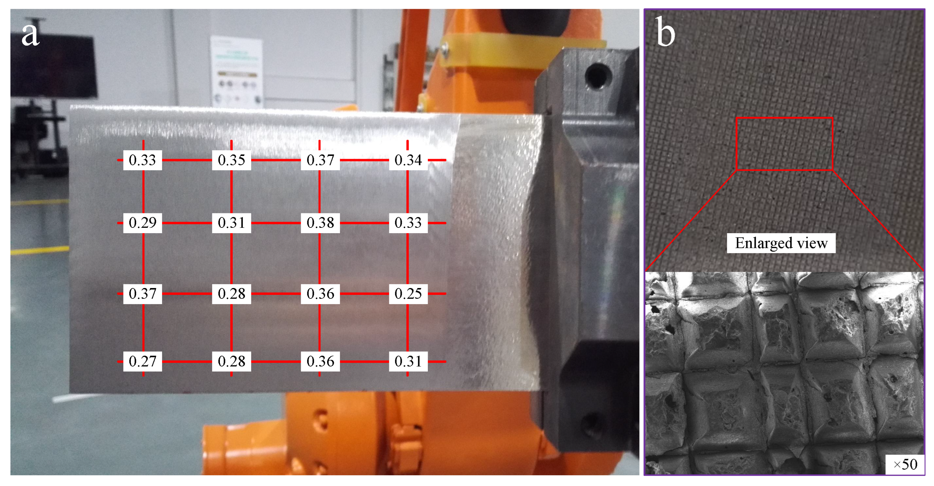
Based on the previously described investigation of IMF energy and its material removal rate, appropriate grinding parameters are selected at $v_s$ = 16.75 m/s, $v_r$ = 40 mm/s, $H_c$ = 30 HRC, and $F_n$ = 50 N in order to guarantee machining stability as well as enhance energy efficiency in the robotic abrasive grinding of the test workpiece. A surface roughmeter (Mitutoyo SJ-210, Mitutoyo, Kawasaki, Japan) with an evaluation length of 4mm and a Gaussian −50% filter was used to obtain the machined workpiece surface roughness values (Ra < 0.4 $\mathsf{\mu }$m), which demonstrate that the workpiece surface is smooth and fine without any machining marks or traces (Figure 18a). The morphology of abrasive belt wear after robotic grinding of a TC4 workpiece is illustrated in Figure 18b. The abrasive belt is currently at the steady wear stage, indicating that its overall wear is more constant and uniform. As observed in Figure 18a, it has a significant capacity for material removal at this stage and can achieve the perfect machining result with appropriate process parameters.

For the roughness statistics in Figure 18a, each location was measured three times ($n=3$), and the plotted value is the arithmetic mean. The 16 location means are summarized in

Table 1. Roughness values (Ra, $\mathsf{\mu }$m) from Figure 18a and statistical summary.

Ra Values at 16 Locations ($\mathbf{\mu }$m)				Indicator	Value
0.33	0.35	0.37	0.34	Overall mean	0.3238
0.29	0.31	0.38	0.33	Standard deviation	0.0406
0.37	0.28	0.36	0.25	Min	0.25
0.27	0.28	0.36	0.31	Max	0.38

. Based on these values, the overall mean roughness is 0.3238 $\mathsf{\mu }$m and the sample standard deviation is 0.0406 $\mathsf{\mu }$m. Furthermore, considering that the present process adopts a 3M structured abrasive belt, the resulting directional topography may have functional implications beyond roughness control. Recent multiscale wettability research indicates that anisotropic and fractal-like surface geometries can significantly influence contact-angle hysteresis, liquid transport behavior, and tribological interactions. Therefore, the textured morphology generated by robotic abrasive-belt grinding is expected to be relevant for applications involving lubrication management, liquid drainage, and surface functionalization [34]. For repeated verification ($n=3$), the normalized abrasive-belt service-life gain was $20.1\%\pm 1.8\%$ and the machining-efficiency gain was $11.9\%\pm 1.4\%$ (mean ± standard deviation), consistent with the improvement range reported in this work.

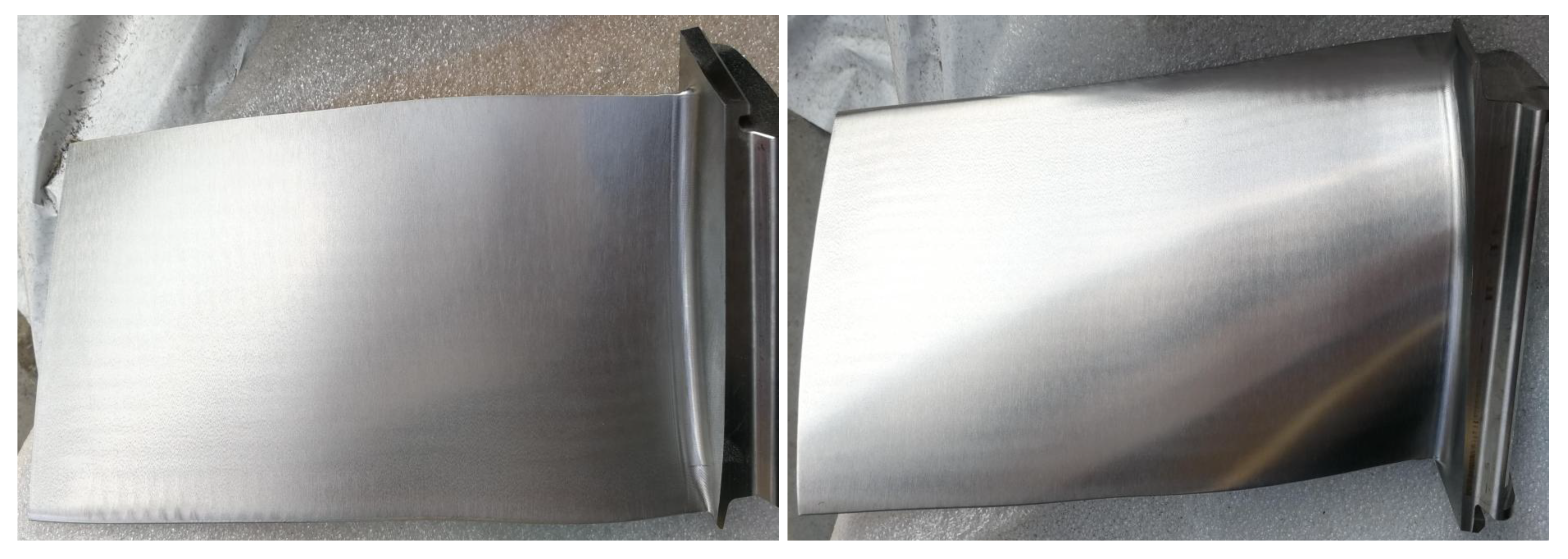
The machining effect of the convex and concave surfaces of a thin-walled blade is depicted in Figure 19 using the following process parameters: $v_s$ = 16.75 m/s, $v_r$ = 60 mm/s, $H_c$ = 30 HRC, and $F_n$ = 20 N. The grinding marks on the blade have clearly been eliminated, and the robotic grinding process has culminated in a smooth, shining blade surface without over-grinding or under-grinding phenomena. On the other hand, the average surface roughness Ra < 0.4 $\mathsf{\mu }$m for the convex and concave surfaces would be in accordance with the actual machining requirements. The quantity of blade scrap caused by excessive belt wear may be decreased by tracking the abrasion of the abrasive belt in real-time. Additionally, a brand-new 3M pyramid belt’s effective service life is extended by approximately 20%, while the machining efficiency is further increased by approximately 12% with the optimization of the IMF components and the three stages of robotic belt cutting action. This significantly extends the abrasive belt’s service life while ensuring the surface quality of the aero-engine blades.

4. Conclusions

A novel AE signal processing algorithm is proposed to demonstrate its characteristics and grinding mechanism, addressing the non-steady state signal of a nonlinear system, and achieving the online monitoring of robotic grinding of titanium alloy workpieces. The following conclusions are achieved:

(1)

The frequency distributions of the IMF1 and IMF3 components span 10–50 kHz and 100–200 kHz, respectively, while IMF2 occupies an intermediate band between IMF1 and IMF3, exhibiting closer spectral proximity to IMF3. Consequently, IMF1, IMF2, and IMF3 can be robustly associated with cutting, plowing, and sliding actions, respectively.

(2)

Under constant normal force, the energy of IMF1 decreases progressively with machining time, whereas both IMF2 and IMF3 energies increase, and this trend aligns with variations in belt linear velocity and contact wheel hardness.

(3)

Within a specific normal force range, both IMF1 energy and MRR increase with rising normal force. Conversely, an inverse relationship is observed with increasing linear velocity. Furthermore, IMF1 energy and MRR increase as contact wheel hardness rises from 45–60 HRC but remain relatively constant within the 30–45 HRC range.

References

1. Li, Y.; Wang, Z.; Zhu, X.; Cai, W.; Chen, D.; Ma, J.; Xu, X.; Yang, Z.; Song, H.; Wang, W.; et al. State-of-the-art in mobile robot-assisted grinding technologies for large-scale complex components. Robot. Comput.-Integr. Manuf. 2026, 101, 103297. [Google Scholar] [CrossRef] [Scilit]
2. Li, L.; Ren, X.; Feng, H.; Chen, H.; Chen, X. A novel material removal rate model based on single grain force for robotic belt grinding. J. Manuf. Process. 2021, 68, 1–12. [Google Scholar] [CrossRef] [Scilit]
3. Xu, B.; Zhang, X.; Yang, Z.; Wang, J.; Yan, S.; Ding, H. Dual flexible contact material removal model for robotic disk grinding. J. Manuf. Process. 2024, 124, 867–876. [Google Scholar] [CrossRef] [Scilit]
4. Yang, Z.; Xu, X.; Li, J.; Zhu, D.; Yan, S.; Ge, S.S.; Ding, H. Knowledge-wrapping method for prediction and evaluation of material removal behavior in robotic belt grinding. Mech. Syst. Signal Process. 2024, 208, 110914. [Google Scholar] [CrossRef] [Scilit]
5. Zhu, D.; Feng, X.; Xu, X.; Yang, Z.; Li, W.; Yan, S.; Ding, H. Robotic grinding of complex components: A step towards efficient and intelligent machining—Challenges, solutions, and applications. Robot. Comput.-Integr. Manuf. 2020, 65, 101908. [Google Scholar] [CrossRef] [Scilit]
6. Zhang, Y.; Liu, H.; Cheng, W.; Hua, L.; Zhu, D. A novel trajectory planning method for robotic deburring of automotive castings considering adaptive weights. Robot. Comput.-Integr. Manuf. 2024, 86, 102677. [Google Scholar] [CrossRef] [Scilit]
7. Xu, X.; Yang, Z.; Liu, Q.; Yan, S.; Ding, H. Condition monitoring and mechanism analysis of belt wear in robotic grinding of TC4 workpiece using acoustic emissions. Mech. Syst. Signal Process. 2023, 188, 109979. [Google Scholar] [CrossRef] [Scilit]
8. Mao, S.H.; Ye, S.T.; Jiang, Y.R.; Shen, C.Q.; Zhang, X.J.; Yan, S.J.; Ding, H. On the existence of mode-coupling chatter in robotic milling based on chatter type indicators extracted by dynamic mode decomposition. Mech. Syst. Signal Process. 2024, 220, 111591. [Google Scholar] [CrossRef] [Scilit]
9. Liu, J.; Ma, C.; Wang, S. Data-driven thermally-induced error compensation method of high-speed and precision five-axis machine tools. Mech. Syst. Signal Process. 2020, 138, 106538. [Google Scholar] [CrossRef] [Scilit]
10. Pandiyan, V.; Tjahjowidodo, T. Use of acoustic emissions to detect change in contact mechanisms caused by tool wear in abrasive belt grinding process. Wear 2019, 436–437, 203047. [Google Scholar] [CrossRef] [Scilit]
11. Caesarendra, W.; Kosasih, B.; Tieu, A.K.; Zhu, H.; Moodie, C.A.; Zhu, Q. Acoustic emission-based condition monitoring methods: Review and application for low speed slew bearing. Mech. Syst. Signal Process. 2016, 72–73, 134–1595. [Google Scholar] [CrossRef] [Scilit]
12. Cheng, C.; Li, J.; Liu, Y.; Nie, M.; Wang, W. An online belt wear monitoring method for abrasive belt grinding under varying grinding parameters. J. Manuf. Process. 2020, 50, 80–89. [Google Scholar] [CrossRef] [Scilit]
13. Chen, J.; Chen, H.; Xu, J.; Wang, J.; Zhang, X.; Chen, X. Acoustic signal-based tool condition monitoring in belt grinding of nickel-based superalloys using RF classifier and MLR algorithm. Int. J. Adv. Manuf. Technol. 2018, 98, 859–872. [Google Scholar] [CrossRef] [Scilit]
14. Zhang, X.; Chen, H.; Xu, J.; Song, X.; Wang, J.; Chen, X. A novel sound-based belt condition monitoring method for robotic grinding using optimally pruned extreme learning machine. J. Mater. Process. Technol. 2018, 260, 9–19. [Google Scholar] [CrossRef] [Scilit]
15. Peta, K.; Suszyński, M.; Wiśniewski, M.; Mitek, M. Analysis of Energy Consumption of Robotic Welding Stations. Sustainability 2024, 16, 2837. [Google Scholar] [CrossRef] [Scilit]
16. Lathi, B.P. Linear Systems and Signals; Berkeley-Cambridge Press: Cambridge, UK, 2009. [Google Scholar]
17. Lu, M.; Wan, B. Study of high-frequency sound signals for tool wear monitoring in micromilling. Int. J. Adv. Manuf. Technol. 2013, 66, 1785–1792. [Google Scholar] [CrossRef] [Scilit]
18. Lin, Y.; Wu, B.; Chen, C. Characterization of grinding wheel condition by acoustic emission signals. In 2018 International Conference on System Science and Engineering (ICSSE); IEEE: Piscataway, NJ, USA, 2018; pp. 1–6. [Google Scholar]
19. Gao, K.; Chen, H.; Zhang, X.; Ren, X.; Chen, J.; Chen, X. A novel material removal prediction method based on acoustic sensing and ensemble XGBoost learning algorithm for robotic belt grinding of Inconel 718. Int. J. Adv. Manuf. Technol. 2019, 105, 217–232. [Google Scholar] [CrossRef] [Scilit]
20. Yang, Z.; Yu, Z.; Xie, C.; Huang, Y. Application of Hilbert-Huang Transform to acoustic emission signals for burn feature extraction in surface grinding process. Measurement 2014, 47, 14–21. [Google Scholar] [CrossRef] [Scilit]
21. Yan, S.; Xu, X.; Yang, Z.; Zhu, D.; Ding, H. An improved robotic abrasive belt grinding force model considering the effects of cut-in and cut-off. J. Manuf. Process. 2019, 37, 496–508. [Google Scholar] [CrossRef] [Scilit]
22. Yin, S.; Song, D.; Li, J.; He, X.; Qiu, L.; Lou, Q.; Wei, M.; Liu, Y. Research on electromagnetic radiation (EMR) waveform characteristics of coal failure process using Hilbert-Huang transform (HHT). Measurement 2022, 187, 110195. [Google Scholar] [CrossRef] [Scilit]
23. Huang, N.E.; Shen, Z.; Long, S.R.; Wu, M.C.; Shih, H.H.; Zheng, Q.; Yen, N.-C.; Yung, C.; Liu, H. The empirical mode decomposition and the Hilbert spectrum for nonlinear and non-stationary time series analysis. Proc. Math. Phys. Eng. Sci. 1998, 454, 903–995. [Google Scholar] [CrossRef] [Scilit]
24. Tang, Y.W.; Tai, C.C.; Su, C.C.; Chen, C.Y.; Chen, J.F. A correlated empirical mode decomposition method for partial discharge signal denoising. Meas. Sci. Technol. 2010, 21, 085106. [Google Scholar] [CrossRef] [Scilit]
25. Wu, Z.; Huang, N. Ensemble empirical mode decomposition: A noise-assisted data analysis method. Adv. Adapt. Data Anal. 2009, 1, 1–41. [Google Scholar] [CrossRef] [Scilit]
26. Torres, M.E.; Colominas, M.A.; Schlotthauer, G.; Flandrin, P. A complete ensemble empirical mode decomposition with adaptive noise. In IEEE International Conference on Acoustics, Speech and Signal Processing; IEEE: Piscataway, NJ, USA, 2011; pp. 4144–4147. [Google Scholar]
27. Colominas, M.; Schlotthauer, G.; Torres, M. Improved complete ensemble EMD: A suitable tool for biomedical signal processing. Biomed. Signal Process. Control 2014, 14, 19–29. [Google Scholar] [CrossRef] [Scilit]
28. Yeh, J.; Shieh, J.; Huang, N. Complementary ensemble empirical mode decomposition: A novel noise enhanced data analysis method. Adv. Adapt. Data Anal. 2011, 2, 135–156. [Google Scholar] [CrossRef] [Scilit]
29. Wu, Z.; Huang, N. A study of the characteristics of white noise using the empirical mode decomposition method. Proc. Math. Phys. Eng. Sci. 2004, 460, 1597–1611. [Google Scholar] [CrossRef] [Scilit]
30. Chu, Y.; Yan, S.; Yang, Z.; Xu, X.; Wang, H.; Ding, H. Grain shape-protrusion-based modeling and analysis of material removal in robotic belt grinding. J. Manuf. Process. 2024, 110, 211–223. [Google Scholar] [CrossRef] [Scilit]
31. Xu, X.; Chu, Y.; Zhu, D.; Yan, S.; Ding, H. Experimental investigation and modeling of material removal characteristics in robotic belt grinding considering the effects of cut-in and cut-off. Int. J. Adv. Manuf. Technol. 2020, 106, 1161–1177. [Google Scholar] [CrossRef] [Scilit]
32. Xu, X.; Ye, S.; Yang, Z.; Yan, S.; Zhu, D.; Ding, H. Analysis and prediction of surface roughness for robotic belt grinding of complex blade considering coexistence of elastic deformation and varying curvature. Sci. China Technol. Sci. 2021, 64, 957–970. [Google Scholar] [CrossRef] [Scilit]
33. Huang, Y.; Wu, Y.; Xiao, G.; Zhang, Y.; Wang, W. Analysis of abrasive belt wear effect on residual stress distribution on a grinding surface. Wear 2021, 486–487, 204113. [Google Scholar] [CrossRef] [Scilit]
34. Peta, K.; Kubiak, K.J.; Brown, C.A. Multiscale geometric analysis of dynamic wettability on complex, fractal-like, anisotropic surfaces. Measurement 2026, 264, 120328. [Google Scholar] [CrossRef] [Scilit]
Figure 1. AE signal characteristics of robotic belt grinding for titanium alloy workpiece.
Machines 14 00501 g001
Figure 2. Schematic of Hilbert–Huang transform (HHT) method.
Machines 14 00501 g002
Figure 3. Schematic of the CEEMDAN method.
Machines 14 00501 g003
Figure 4. Schematic of the proposed CCEEMD method.
Machines 14 00501 g004
Figure 5. Processing schematic of background noise in robotic belt grinding experiments: (a) original noise and eliminated idle noise; (b) sample signal.
Machines 14 00501 g005
Figure 6. Mode function “energy-period” logarithmic distribution of background noise.
Machines 14 00501 g006
Figure 7. Change of m-order IMF component energy and proportion C ( m ) in its total energy.
Machines 14 00501 g007
Figure 8. Schematic of AE signal denoising algorithm based on noise statistical characteristics.
Machines 14 00501 g008
Figure 9. Schematic of robotic grinding system (a) and AE signal processing system (b).
Machines 14 00501 g009
Figure 10. Acquired AE signal (a) and truncated waveform (b) with parameters: normal force F n = 50 N, belt velocity v s = 16.75 m/s, feed speed v f = 5 mm/s, and contact hardness H c = 30 HRC.
Machines 14 00501 g010
Figure 11. The first 8-order IMFs of the AE signal after decomposition of the proposed method.
Machines 14 00501 g011
Figure 12. Time and marginal spectrum of AE signal by Hilbert–Huang transform.
Machines 14 00501 g012
Figure 13. Log period and energy distribution of each IMF component of AE signals.
Machines 14 00501 g013
Figure 14. Marginal spectrum of the first three-order IMF components and their sum Σ IMF.
Machines 14 00501 g014
Figure 15. Variation curves under different normal forces: (a) IMF1 energy versus machining time; (b) IMF2 energy versus machining time; (c) IMF3 energy versus machining time; (d) material removal rate versus machining time.
Machines 14 00501 g015
Figure 16. Variation in IMF energy and material removal rate under different belt linear velocities: (a) IMF1 energy versus machining time; (b) IMF2 energy versus machining time; (c) IMF3 energy versus machining time; (d) material removal rate versus machining time.
Machines 14 00501 g016
Figure 17. Variation in IMF energy and material removal rate under different contact wheel hardness values: (a) IMF1 energy versus machining time; (b) IMF2 energy versus machining time; (c) IMF3 energy versus machining time; (d) material removal rate versus machining time.
Machines 14 00501 g017
Figure 18. The machining effect of the TC4 workpiece: (a) the surface roughness values after robotic abrasive belt grinding; (b) the wear degree of a 3M pyramid belt.
Machines 14 00501 g018
Figure 19. The robotic grinding effect of a convex and concave surface of an aero-engine blade.
Machines 14 00501 g019