1. Introduction
The Job Shop Scheduling Problem (JSP) is a classical combinatorial optimization problem in manufacturing systems. The Flexible Job Shop Scheduling Problem (FJSP) extends JSP by allowing each operation to be processed on one of several alternative machines, which significantly enlarges the search space and increases the complexity of decision-making [
1,
2]. While most early studies focused on single-objective formulations such as makespan minimization, practical production environments usually involve multiple conflicting objectives. In particular, with increasing emphasis on due-date compliance and sustainable manufacturing, the Multi-Objective Flexible Job Shop Scheduling Problem (MOFJSP), which simultaneously considers makespan (MT), total tardiness (TT), and total energy consumption (TE), has become more relevant to real industrial requirements [
3].
Existing studies on MOFJSP are still dominated by metaheuristic methods, especially multi-objective evolutionary algorithms (MOEAs) [
4]. These methods are effective for global search and can provide high-quality approximations to the Pareto front. However, they typically rely on repeated population evolution and large numbers of objective evaluations, which lead to considerable computational cost. As a result, although MOEAs remain strong offline optimizers, their iterative search nature limits their applicability in time-sensitive manufacturing scenarios that require rapid scheduling responses.
Deep reinforcement learning (DRL) provides a different paradigm. By learning a policy through repeated interactions with the environment during training, DRL can make scheduling decisions efficiently at inference time through direct policy rollout, which makes it attractive for online or low-latency scheduling. Recent studies have also shown that combining DRL with graph representation learning can improve the modeling of job–machine relationships and support end-to-end decision-making in FJSP [
4,
5]. Nevertheless, for MOFJSP, many existing DRL methods still optimize a fixed scalarized objective or a narrow range of preferences [
1]. Consequently, the learned policy is often tailored to a particular trade-off and cannot directly provide a well-distributed Pareto-front approximation after a single training process.
To address multi-objective decision-making, several DRL-based directions have been explored. PDR-based methods constrain the action space to a predefined set of dispatching rules, which improves interpretability but limits policy expressiveness [
6,
7]. Multi-agent or multi-policy methods decompose the decision process across objectives or subproblems, but often require multiple coordinated policies and may incur additional training and deployment complexity [
8,
9,
10]. More recently, preference-conditioned graph reinforcement learning has shown that a single policy conditioned on a preference vector can rapidly generate Pareto-approximate solution sets for MOFJSP at inference time [
11]. The proposed DPG-GRL follows this general paradigm, but differs from existing methods in the optimization setting and training mechanism. In particular, this work addresses the MT/TT/TE objective setting and introduces a dual-pool-guided proximal policy optimization (PPO) framework to improve sample efficiency and training stability in multi-preference policy learning. In constrained, long-horizon scheduling problems such as MOFJSP, stable and efficient multi-preference learning remains challenging.
Another relevant line of work combines evolutionary algorithms and reinforcement learning. Existing hybrid methods mainly fall into two categories. In the first category, RL is used to adaptively control evolutionary search, for example by selecting operators or tuning hyperparameters during optimization [
12]. In the second category, high-quality solutions generated by EAs are used to guide RL training and improve learning efficiency [
13]. Although these studies demonstrate the potential of combining search-based and learning-based paradigms, most of them focus on single-objective FJSP or dynamic scheduling settings. For MOFJSP, what is still lacking is a more stable and sample-efficient preference-conditioned framework that enables a single policy to cover diverse preference trade-offs while remaining practical in deployment.
Accordingly, this paper proposes dual-pool guided preference-conditioned graph reinforcement learning (DPG-GRL) for MOFJSP. The proposed method learns a single preference-conditioned policy that can generate scheduling solutions with different trade-offs under different preference vectors. To improve sample efficiency and training stability, we further introduce a dual-pool guidance mechanism. Specifically, an offline expert pool provides a stable behavioral prior through replayed demonstration trajectories, while an online elite pool continuously replays high-quality trajectories generated by the current policy for self-improving refinement. In this way, DPG-GRL combines graph-based structured state encoding, preference-conditioned policy learning, and experience-guided training within a unified framework for fast Pareto-front approximation.
The main contributions of this study are summarized as follows.
- (1)
We develop a distinct preference-conditioned graph reinforcement learning framework for MOFJSP that combines heterogeneous operation–machine modeling and PPO-based optimization for Pareto approximation under multiple preferences.
- (2)
We introduce a dual-pool guidance mechanism that combines offline expert demonstrations and online elite replay to improve sample efficiency and training stability during multi-preference policy learning.
- (3)
We design a preference-aware encoder–decoder policy with lightweight decoder-level hypernetwork conditioning, which enables preference-sensitive decision-making across trade-offs while preserving a shared graph representation.
- (4)
Experiments on synthetic and public benchmark instances show that the proposed method achieves competitive Pareto approximation quality with clear inference-efficiency advantages.
The rest of this paper is organized as follows.
Section 2 reviews related work.
Section 3 presents the problem formulation and background.
Section 4 describes the proposed method.
Section 5 reports the experimental results and analysis.
Section 6 concludes the paper and outlines directions for future research.
2. Related Work
The MOFJSP is typically addressed as a Pareto optimization problem that seeks a set of non-dominated trade-off solutions rather than a single optimum [
14]. Existing studies can be broadly grouped into three categories: metaheuristic methods, DRL-based methods, and hybrid methods that combine evolutionary search and reinforcement learning. The following review focuses on representative directions most relevant to this work.
2.1. Metaheuristic Methods
Metaheuristic algorithms, especially evolutionary algorithms, have long been the dominant approach for MOFJSP because they are well suited to approximating Pareto fronts and producing multiple trade-off solutions in a single run. Representative studies include improved NSGA-II variants for low-carbon flexible job shop scheduling [
15] and neighborhood-enhanced discrete evolutionary methods for real production scheduling scenarios [
16]. These methods often achieve strong global search performance and can produce competitive solution sets across multiple objectives.
Despite their effectiveness, metaheuristic methods still face an inherent limitation in time-sensitive settings. Their performance depends on repeated population evolution, objective evaluations, and parameter tuning, all of which become increasingly expensive as the problem size and constraint complexity grow. Therefore, although MOEAs remain strong baselines for MOFJSP, their iterative search nature limits their suitability for rapid deployment and real-time scheduling.
2.2. Deep Reinforcement Learning Methods
Recent DRL-based methods for production scheduling can be roughly divided into three directions: PDR-based reinforcement learning, multi-agent or multi-policy methods, and graph-based reinforcement learning. These approaches improve decision efficiency in different ways, but their effectiveness for MOFJSP still depends on their ability to balance preference coverage, learning stability, and deployment efficiency.
2.2.1. PDR-Based Reinforcement Learning
PDR-based reinforcement learning methods usually treat the selection of a priority dispatching rule as the core action. This design reduces action-space complexity and offers better interpretability, which is especially useful in dynamic or resource-constrained scheduling scenarios. For example, hybrid deep Q-network methods have been used to select dispatching rules for dynamic FJSP settings with transportation constraints [
17], and PPO-based event-driven rescheduling has been explored to cope with unexpected job arrivals [
18].
However, the performance of such methods is largely constrained by the coverage and expressiveness of the rule library. If promising scheduling decisions are not represented by the predefined rules, the policy cannot discover them directly. This makes it difficult for PDR-based methods to robustly approximate diverse Pareto trade-offs in MOFJSP.
2.2.2. Multi-Agent Methods for MOFJSP
Another important direction is to decompose scheduling decisions into multiple interacting subproblems and solve them through multi-agent or multi-policy learning. In dynamic MOFJSP settings, multi-agent frameworks have been used to separately model coupled decisions such as job selection and machine assignment [
9]. Collaborative multi-agent reinforcement learning has also been introduced to balance different objective preferences, such as makespan and energy consumption, through weight-allocation mechanisms [
19]. In addition, multi-policy deep reinforcement learning has been proposed to learn multiple policies under different objective weights and jointly approximate Pareto trade-offs [
8].
These methods improve flexibility and policy expressiveness by decomposing the learning task. However, they often rely on multiple coordinated policies or agents, which can increase training complexity, coordination instability, and deployment cost. More importantly, they do not directly address how to learn a single stable policy that generalizes well across diverse preference trade-offs.
2.2.3. Graph-Based Deep Reinforcement Learning
Graph Reinforcement Learning (GRL) models shop-floor states as disjunctive or heterogeneous graphs and leverages graph neural networks (GNNs) to learn structured representations for end-to-end scheduling decisions [
5]. For green and low-carbon FJSP, ref. [
1] adopted a disjunctive-graph representation and proposed a graph attention-based method to improve generalization. For MOFJSP, ref. [
11] introduced a preference-conditioned GRL approach that uses a single preference-conditioned policy for fast Pareto-approximate solution generation at inference time.
These studies demonstrate that graph-based policy learning is a promising direction for MOFJSP because it can better capture operation–machine coupling and exploit structured representations. However, existing GRL-based methods still often suffer from limited sample efficiency and unstable training, especially when a single policy is required to cover diverse preferences. Relative to Su et al. [
11], the present work considers a different objective setting and adopts a heterogeneous operation–machine graph together with a lightweight decoder-level conditioning strategy. More importantly, it places greater emphasis on sample efficiency and training stability through a dual-pool-guided PPO framework. This motivates the introduction of experience-guided training mechanisms to improve multi-preference policy learning and Pareto-front approximation quality.
2.3. Hybrid Algorithms
To combine the global search capability of evolutionary algorithms with the rapid inference of learned policies, EA-RL hybrid methods have attracted increasing attention. Existing studies mainly follow two routes.
In the first route, referred to here as RL-assisted EA, reinforcement learning is used to guide the evolutionary process, for example by selecting operators or adapting search strategies online [
20,
21]. Such methods can improve the efficiency of evolutionary search, but they still retain the iterative optimization framework of EAs and therefore remain computationally expensive at deployment time.
In the second route, referred to here as EA-assisted RL, high-quality solutions found by evolutionary algorithms are used to guide RL training [
13,
22]. This idea is particularly relevant to scheduling because good solutions can be replayed as demonstrations to reduce early exploration difficulty and improve training stability. However, existing studies of this kind mainly focus on dynamic scheduling or non-MOFJSP variants, and a unified framework for stable multi-preference learning in MOFJSP is still lacking.
In summary, metaheuristic methods can provide high-quality Pareto solutions but are computationally expensive; DRL-based methods enable efficient inference but still struggle with preference coverage and training stability in MOFJSP; and existing hybrid methods improve learning or search efficiency only partially. To address these limitations simultaneously, this paper proposes DPG-GRL, which combines preference-conditioned graph policy learning with dual-pool guidance to improve both training stability and Pareto-front approximation quality.
4. The DPG-GRL Algorithm for MOFJSP
This section presents the proposed DPG-GRL in detail. For the MOFJSP, DPG-GRL scalarizes multi-objective feedback under a preference vector , decomposing the original problem into a family of preference-dependent subproblems. It then learns a single preference-conditioned policy network that can produce preference-specific decisions for different . After training, inference only requires specifying a set of preference vectors and performing forward inference to rapidly generate scheduling solutions with diverse trade-offs, enabling a unified model to approximate the Pareto front.
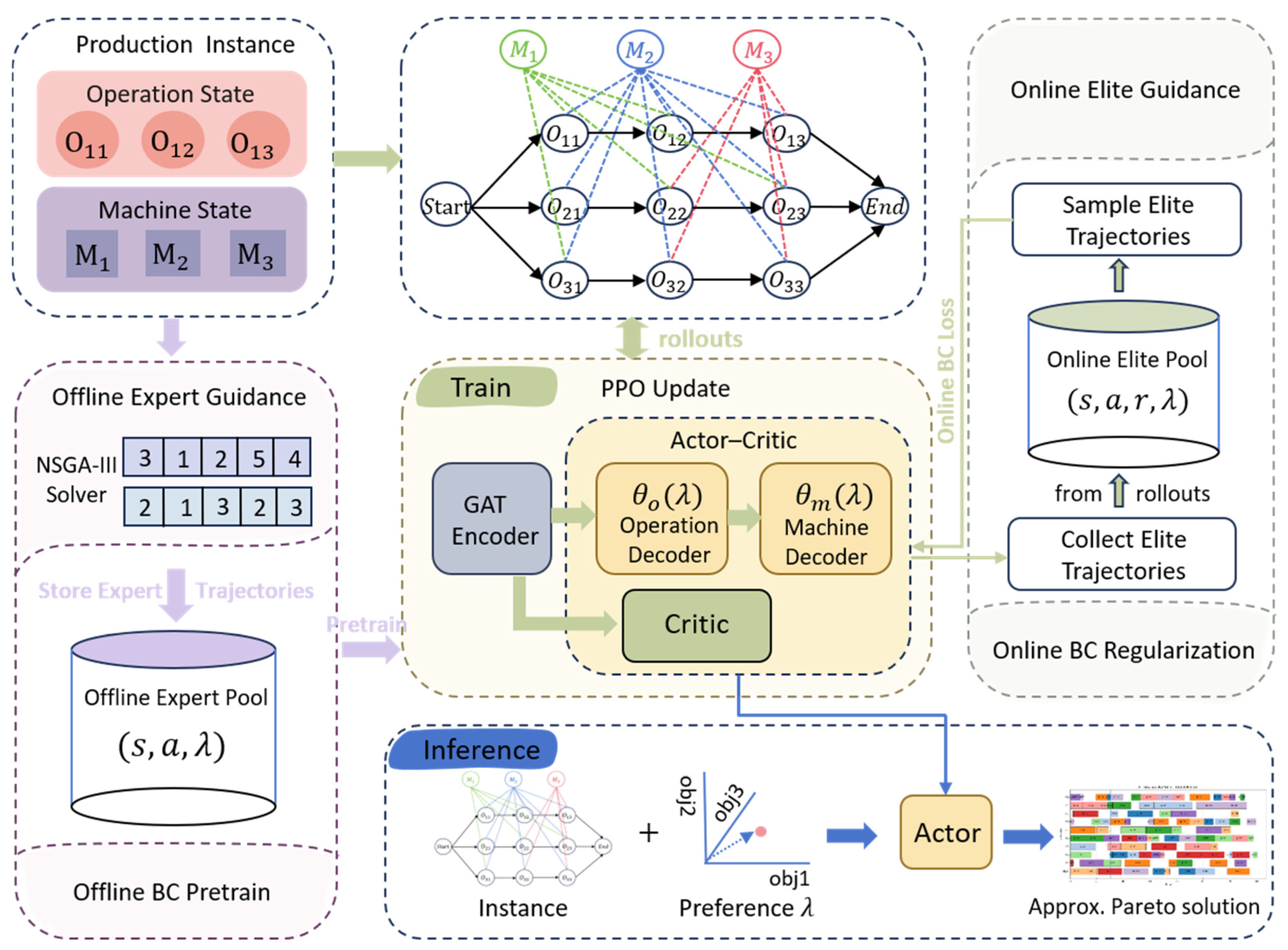
To improve sample efficiency and training stability, DPG-GRL incorporates a dual-pool guidance mechanism. An offline expert pool provides a transferable behavioral prior across preferences for stable initialization, while an online elite pool continuously collects and filters high-quality trajectories generated by the current policy to form self-improving supervision. This mechanism mitigates policy drift and improves training stability during learning. The framework includes an offline stage for expert-pool construction and behavior-cloning initialization, an online stage for PPO rollout and elite-pool update, and an inference stage in which the trained policy is executed under a set of preference vectors to generate a Pareto-approximate solution set. The overall workflow is illustrated in
Figure 2.
4.1. MDP Formulation of MOFJSP
We formulate the MOFJSP as a multi-objective Markov decision process. Given a preference weight vector over the three objectives, the problem under a fixed is represented by the tuple At each decision step , the agent selects an action based on the current state , and the environment transitions to the next state according to . This process continues until all operations have been scheduled and the terminal state is reached.
To enable a single policy to exhibit differentiated behaviors under different preferences, we apply preference-conditioned scalarization during learning and convert the multi-objective feedback into a scalar reward under , which can be directly used for reinforcement learning updates. The MDP components and the corresponding policy are defined as follows.
4.1.1. State
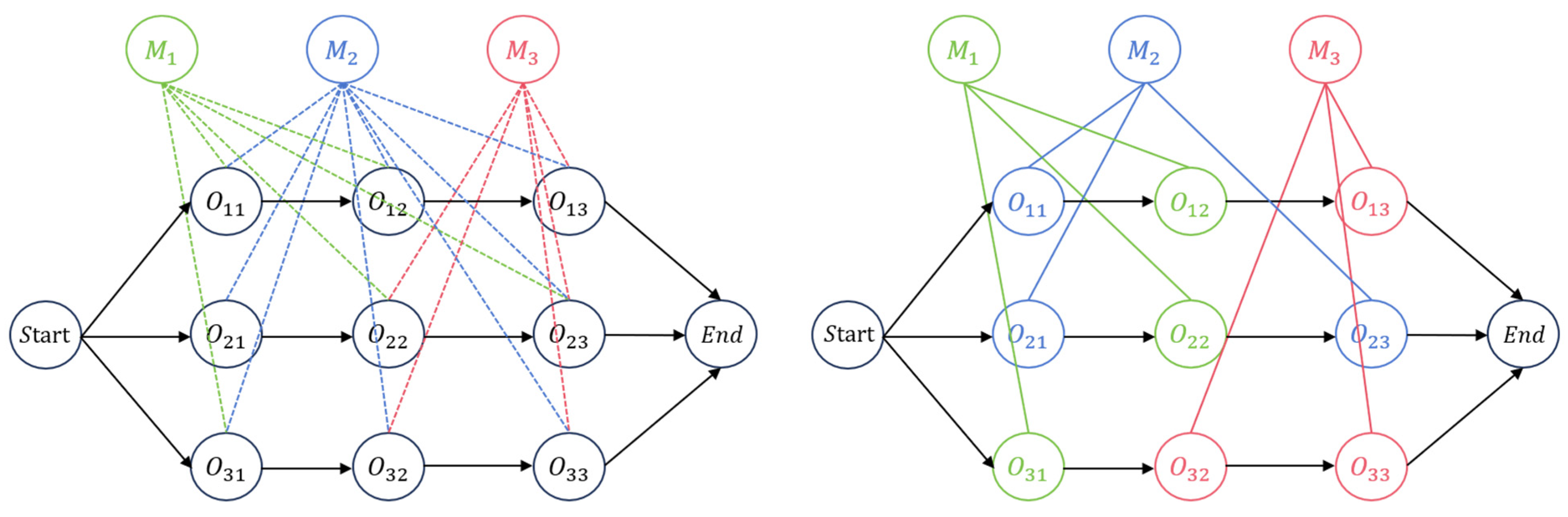
The state should jointly represent the features of both operations and machines. To this end, we model as a decision-evolving heterogeneous graph . The graph contains two types of nodes, operation nodes and machine nodes , as well as two types of edges: precedence edges between consecutive operations and operation–machine feasibility edges. For an operation node , the raw features include a readiness indicator and a scheduling indicator . For a machine node , the features mainly include the machine availability time and statistics related to the current workload.
4.1.2. Action
In MOFJSP, each decision is naturally decomposed into two steps: selecting an operation and then assigning an eligible machine to the selected operation. Accordingly, the action at decision step is defined as where denotes the selected operation and denotes the eligible machine assigned to that operation.
4.1.3. State Transition
After the agent executes an action in state , the environment advances the schedule by one step and updates the associated state features, resulting in the next state .
4.1.4. Reward
Because MT and TT can only be computed exactly after a complete schedule is obtained, constructing rewards directly from these global objectives would yield extremely sparse feedback and may undermine the training stability of proximal policy optimization (PPO). To address this issue, we transform MT and TT into dense feedback using difference-based reward shaping: after executing action in state and transitioning to , we define , ; here, is defined as the maximum estimated completion time across all jobs under the current partial schedule, and is defined as the estimated total tardiness under the current partial schedule. In contrast, the energy-related component is computed directly from the environment. To eliminate scale differences across objectives, each raw component is normalized as , where denotes the objective-specific scale factor estimated from the running statistics of the corresponding reward component during training. This normalization is used to reduce numerical-scale imbalance among MT, TT, and TE.
The proposed reward design is intended to alleviate the long-horizon credit assignment problem caused by sparse terminal feedback in MOFJSP. In particular, the difference-based shaping terms provide stepwise signals related to the marginal improvement in the current partial schedule. Given a preference vector , the scalar reward is then computed as , and is used for PPO in the two-stage decision-making process.
4.1.5. Policy
Based on the above definitions of states and actions, we learn a preference-conditioned policy that takes as input. To match the two-step action structure, the policy is parameterized in a hierarchical manner. First, the operation-selection policy outputs a probability distribution over candidate operations, from which an operation is selected. Then, conditioned on the selected operation, the machine-selection policy outputs a probability distribution over feasible machines, from which a machine is chosen.
The two-stage decisions share the same graph-encoded representation and incorporate the preference vector , enabling a single set of network parameters to produce differentiated scheduling behaviors under different preferences.
4.2. Preference-Conditioned Graph Policy Network
Accordingly, we parameterize the policy of the MOMDP using a preference-conditioned graph policy network. Given the scheduling state
and preference vector
, the network outputs a two-stage action
, corresponding to operation selection and feasible machine assignment, respectively. The overall policy is factorized as
The network consists of a preference-agnostic heterogeneous-graph encoder and two preference-aware decoders. At decision step
, the encoder maps the heterogeneous graph into a shared embedding that captures instance-specific information. Following Navon et al. [
26], we introduce a hypernetwork [
27] to generate the parameters of decoder-related layers, allowing the decoder to condition on
and produce differentiated decisions under different trade-offs. Unlike approaches that condition the entire network on
[
26], we condition only the final linear layer of each decoder while sharing all other layers. This design reduces the number of preference-conditioned parameters while preserving expressiveness across preferences and improving training stability.
4.2.1. Graph Attention Network Encoder
At decision step , the MOFJSP state is represented as a heterogeneous graph , where and denote the sets of operation nodes and machine nodes, respectively. The edge set represents technological precedence relations among operations, and denotes operation–machine feasibility relations. Node features are provided by the state-construction module. For operation–machine edges, edge attributes include assignment-related information such as processing time.
We adopt a graph attention network (GAT) [
28] with relation-specific parameters to model different edge types. For an edge
under relation
, let
and
be the representations of the source and target nodes, and let
denote the edge feature. The unnormalized attention score and its normalized coefficient are computed as
where
denotes the set of neighbors with edges pointing to node
under relation
. The target node is then updated via weighted aggregation:
where
and
is an activation function.
By stacking multiple heterogeneous attention layers, we obtain the operation embedding matrix and the machine embedding matrix . The node embeddings can also be pooled to form a global graph representation , which provides global context to the decoders. The encoder parameters are independent of the preference vector and the same encoder is shared across different preferences to provide stable structural representations.
4.2.2. Preference-Aware Decoder
The encoder outputs
, which are shared by the two decoders. To realize preference conditioning, we employ a hypernetwork to generate the parameters of the final linear layer in each decoder, while all preceding layers are shared. This design reduces the conditioning overhead and improves training stability. For each decoder
, let
denote the output of the shared multilayer perceptron (MLP) trunk. The hypernetwork takes the preference vector
as input and produces the parameters of the last scoring layer. Specifically, the hypernetwork output is computed by
where
denotes the trainable parameter set of the hypernetwork associated with decoder
. Since
,
and
correspond to the hypernetworks for the operation-selection decoder and the machine-assignment decoder, respectively. The weight vector and bias of the final linear layer are then generated as
where
. The resulting logit is
With this formulation, different preferences induce different action scores by modifying only the final layer, which enables a single network to generate Pareto-approximate solution sets across multiple preferences.
Operation-selection decoder. The operation-selection decoder
is implemented as an MLP that outputs a distribution over the candidate set
at step
. Consistent with the implementation, we extract the embedding of the current operation of each job, denoted by
from
and concatenate it with the global representation:
The shared MLP trunk maps
to
, and the hypernetwork module in (17)–(19) produces the corresponding logit
. We then mask out infeasible operations [
29] and apply a masked softmax over the remaining logits to obtain the operation-selection policy:
Machine-assignment decoder. Similarly, the machine-assignment decoder
outputs a distribution over the feasible machine set
after an operation
is selected. For each machine
k, we construct the candidate feature vector as
where
is the embedding of the selected operation and
summarizes assignment-related information. The machine-selection policy is obtained by masking infeasible machines and normalizing over the feasible machine set
.
With the preference-conditioned dual decoders, inference only requires changing the preference vector to generate scheduling action sequences with different trade-offs using a single policy network, thereby achieving broad coverage across preferences and approximating the Pareto front efficiently.
4.3. Dual-Pool Guidance Mechanism
Although a preference-conditioned policy can cover different trade-offs with a single model at inference time, purely on-policy training in MOFJSP—featuring long decision horizons and stringent feasibility constraints—often suffers from low exploration efficiency, high gradient variance, and policy drift. To mitigate these issues, we introduce a dual-pool guidance mechanism. Specifically, an offline expert pool provides a transferable behavioral prior for stable initialization, while an online elite pool continuously filters and replays high-quality trajectories generated by the current policy to refine the policy and stabilize learning, thereby improving sample efficiency and convergence performance.
4.3.1. Offline Expert Pool
The offline expert pool
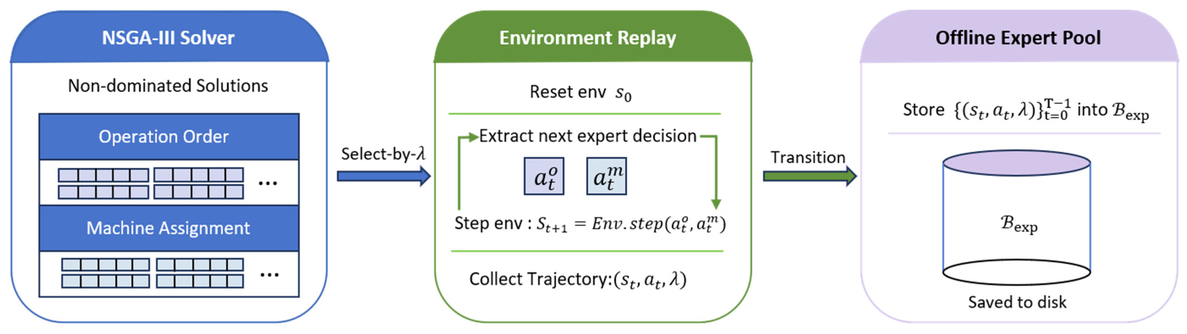
transforms high-quality scheduling solutions produced by a multi-objective solver into supervised data that can be directly learned by the preference-conditioned policy, thereby providing a stable behavioral prior. As illustrated in
Figure 3, we first run NSGA-III on the training instances to obtain a set of non-dominated solutions, where each solution specifies both an operation sequence and a machine assignment. Given a preference vector
, we then select a solution that matches the corresponding trade-off from this set and deterministically reconstruct it into a step-by-step decision trajectory through environment replay. Starting from the initial state
, at each decision step we extract the action
that is consistent with the selected expert solution and advance the environment to the next state,
. During replay, tuples
are recorded, and the resulting trajectories are stored in
as an offline demonstration dataset that can be repeatedly sampled.
The offline expert pool is used for behavior-cloning initialization in the early stage of training, which alleviates insufficient exploration and policy drift. It also provides a stable supervised regularization signal for subsequent on-policy optimization.
4.3.2. Online Elite Pool
The online elite pool is designed to continuously select high-quality samples from trajectories generated by the current policy and use them as supervised signals for an online behavior-cloning regularizer, enabling self-improvement. To prevent the pool from degenerating into a short-term buffer that only reflects the most recent data distribution, we maintain an external elite archive and adopt a top- truncated update scheme, so that the stored samples preserve elite quality while retaining a certain level of diversity over time.
In each update cycle, the policy performs rollouts under preferences sampled from We collect the terminal schedules produced by these rollouts and their objective vectors to form a candidate set . The candidates are first filtered by non-dominance to obtain . Given a preference vector , we compute the corresponding scalarized score for each solution, rank the solutions accordingly, and retain the top- solutions to form the elite set . The trajectories associated with elite solutions are then converted into tuples and stored in . When the pool reaches its maximum capacity, lower-scoring samples are evicted using the same scoring criterion. The resulting elite replay provides a continual source of high-quality supervision that regularizes PPO updates, thereby improving training stability and solution quality.
4.4. Two-Stage Training and Online Inference
To learn a stable single-policy model for MOFJSP under diverse preferences, we adopt a two-stage training and one-pass inference paradigm. The policy is first initialized from offline expert demonstrations and is then optimized mainly by PPO through online interactions. During online training, behavior-cloning regularization from both the offline expert pool and the online elite pool is introduced to reduce policy drift and improve sample efficiency. After training, inference only requires sweeping a set of preference vectors to generate a Pareto-approximate solution set without additional search.
For clarity, the dual-pool-guided learning procedure consists of five steps. First, an offline expert pool is constructed by solving the training instances with NSGA-III and replaying selected high-quality solutions into stepwise demonstration trajectories. Second, the preference-conditioned policy is initialized by behavior cloning on these expert samples. Third, PPO rollouts are performed under sampled preference vectors to collect on-policy trajectories. Fourth, the terminal solutions generated by the current policy are filtered by non-dominance and preference-conditioned ranking, and the corresponding top- trajectories are written into the online elite pool. Fifth, the policy is updated using the PPO objective together with behavior-cloning regularization from both pools. In this way, the offline pool provides stable early guidance, while the online pool supplies evolving high-quality supervision during later training.
4.4.1. Offline Expert Pretraining
Offline pretraining is performed on the Expert Pool to obtain an initial policy that produces feasible schedules and captures reasonable decision patterns across multiple preferences. For each supervised sample, the action is decomposed into two stages,
, corresponding to operation selection and machine assignment. Pretraining minimizes the negative log-likelihood of the demonstrated two-stage actions, encouraging the policy to reproduce expert decisions conditioned on the state and the preference vector. This initialization reduces exploration noise in the early phase and improves the stability of subsequent on-policy learning (Algorithm 1).
| Algorithm 1: Two-stage training procedure of DPG-GRL |
| Require: preference-conditioned policy ; critic , ExpertPool capacity , ElitePool capacity , BC pretrain epochs , PPO iterations , rollout horizon T, PPO epochs K; elite size , BC weights , validation period |
| 1: Build ExpertPool with capacity via NSGA-III solutions and trajectory replay (Algorithm 2) |
| 2: Stage I: Offline expert pretraining |
| 3: for epoch = 1 to do |
| 4: Sample supervised batch ~ |
| 5: Update by minimizing |
| 6: end for |
| 7: Stage II: Online RL with dual-pool guidance |
| 8: for iter = 1 to do |
| 9: Sample preference vectors from Dirichlet for parallel rollouts |
| 10: Collect on-policy batch by rolling out for horizon T |
| 11: Update ElitePool using candidate rollouts and (Algorithm 2) |
| 12: Compute PPO loss with -conditioned scalar advantage |
| 13: Sample ~ ElitePool and ~ |
| 14: Compute BC regularizers |
| 15: Update by minimizing |
| 16: if iter mod then evaluate HV on ; save best model |
| 17: end for |
| 18: Output: and critic |
4.4.2. Online PPO with Dual-Pool Regularization
In the online stage, the policy interacts with the environment under preferences sampled from the distribution
to collect an on-policy batch
, which is used for PPO updates. Meanwhile, supervised batches
and
are sampled from the offline expert pool and the online elite pool, respectively, to construct behavior-cloning regularizers that are optimized jointly with the PPO objective. Here,
denotes the parameters of the preference-conditioned actor policy
= (
,
), including the encoder, the two decoders, and the decoder-level hypernetwork modules. In addition,
denotes the parameters of the critic/value network
. The resulting joint objective is
where
and
control the strengths of the two guidance sources, allowing learning to transition from demonstration-based regularization in the early stage to return-driven policy improvement in the later stage. In this formulation, the two behavior-cloning terms serve as auxiliary regularizers of the PPO objective and provide expert-guided and self-improving supervision during policy learning. Consistent with the two-stage action structure, the behavior-cloning loss is defined as
where
and
denote the policy distributions for operation selection and machine assignment, respectively.
The online elite pool is updated in each cycle using candidate solutions extracted from rollouts. We first apply non-dominance filtering and then perform top-
truncation based on a preference-conditioned scalarized score. This score adopts the same weighted-sum form used during training and is used to rank candidates under a given
. The trajectories associated with the selected elite solutions are then written into ElitePool to form self-improving supervision (Algorithm 2). In this way, the supervised signal evolves with the current policy, thereby improving training stability and preference coverage.
| Algorithm 2: Dual-pool guidance mechanism of DPG-GRL |
| Require: NSGA-III solver , expert preference set , ExpertPool capacity , ElitePool capacity , elite size ; scalarization |
| 1: Build ExpertPool |
| 2: for each instance do |
| 3: Run NSGA-III solver to obtain a non-dominated set |
| 4: for each do |
| 5: Select representative solution λ |
| 6: Replay λ in the environment to recover stepwise decisions |
| 7: Store supervised tuples into ExpertPool |
| 8: end for |
| 9: end for |
| 10: Update ElitePool per PPO iteration |
| 11: Collect rollout candidates with terminal objectives under current |
| 12: Filter by non-dominated sorting to obtain |
| 13: Score each by |
| 14: Select the top- trajectories with the best scores |
| 15: Insert into ElitePool; if overflow , remove lowest-score items |
| 16: Output: ExpertPool, ElitePool |
4.4.3. Online Inference and Solution-Set Generation
No search is performed during inference. Given a test instance, we construct a deterministic preference set using the Das-Dennis method with 12 partitions, resulting in
preference vectors for the three-objective setting. For each preference vector, we perform a single rollout using the learned policy until termination to obtain a scheduling solution
. All solutions are then aggregated and filtered by non-dominance to produce an approximate Pareto set
(Algorithm 3). Because the policy is preference-conditioned, this procedure provides diverse trade-off solutions with a low and fixed inference cost. The same inference-time preference set is used for all compared methods to ensure fair evaluation.
| Algorithm 3: Online inference for Approximate Pareto Set Generation |
| Require: trained actor policy ; test instance ; preference set |
| 1: Initialize candidate solution set |
| 2: for each do: |
| 3: Reset environment with instance , obtain initial state |
| 4: while is not terminal do |
| 5: Compute graph embedding |
| 6: Select operation |
| 7: Select machine |
| 8: Execute , transition to |
| 9: end while |
| 10: Obtain terminal objective vector ; add solution to |
| 11: end for |
| 12: |
| 13: Output: approximate Pareto set for . |
For clarity,
Figure 2 provides the conceptual workflow of the proposed framework, whereas Algorithms 1–3 summarize its executable procedures at three different levels. Algorithm 1 describes the overall two-stage training process, Algorithm 2 details the construction and update of the dual-pool guidance mechanism, and Algorithm 3 summarizes the inference-time generation of the approximate Pareto set.
Algorithm 1 presents the complete training procedure of DPG-GRL. Its main purpose is to show how offline expert pretraining and online PPO are integrated within a unified learning framework. In particular, the algorithm highlights that the ExpertPool is first constructed and used for behavior-cloning initialization, after which PPO rollouts, ElitePool update, and dual-pool-regularized policy optimization are performed iteratively.
Algorithm 2 presents the dual-pool guidance mechanism in greater detail. The offline part explains how representative solutions obtained by NSGA-III are transformed into replayable expert trajectories, while the online part shows how elite trajectories are selected from current policy rollouts through non-dominance filtering and preference-conditioned top- selection. This algorithm therefore clarifies how the two pools are constructed from different sources and how they provide complementary supervision during training. Here, denotes the expert preference set used to select representative solutions from the NSGA-III-generated non-dominated set during ExpertPool construction; each is a non-negative three-objective preference vector satisfying + TT + TE = 1. The parameter denotes the number of top-ranked elite trajectories retained in each ElitePool update.
Algorithm 3 presents the inference-time generation of the approximate Pareto set. Its main purpose is to show how the trained preference-conditioned policy is deployed after training. In particular, for each preference vector in the deterministic preference set, the policy performs one rollout on the test instance to generate a candidate scheduling solution, after which all candidate solutions are filtered by non-dominance to obtain the final approximate Pareto set.
5. Experiments
To systematically evaluate the proposed DPG-GRL, we conduct experiments on synthetic instances and standard public benchmark instances, and compare DPG-GRL against representative baselines in terms of solution quality and computational efficiency. We further perform ablation studies by removing offline expert pretraining and the online elite pool, respectively, to quantify the contribution of each component in the dual-pool guidance mechanism to convergence speed and final Pareto-front approximation quality. All experiments are conducted on a server equipped with an AMD EPYC 9754 CPU (Advanced Micro Devices, Inc., Santa Clara, CA, USA) and an NVIDIA RTX 4090 GPU (NVIDIA Corporation, Santa Clara, CA, USA).
5.1. Experimental Settings
5.1.1. Datasets
We construct synthetic instances at three scales: 10 × 5, 10 × 10, and 15 × 15. Instance generation follows the setting in [
14]. Specifically, an n × m instance contains
jobs and
machines, and the number of operations in each job is set equal to the number of machines. The processing time
is sampled from a uniform distribution
. To construct the total tardiness (TT) and total energy consumption (TE) objectives, we additionally generate job due dates and assign power parameters to machines. The due date
is generated using the classical procedure in [
30], where the due-date generation rule is set to tf_rdd with TF = 0.3 and RDD = 1.3. The processing power
of each machine is sampled from
, and the idle power is set to
, where
= 0.2. The transportation energy
is fixed to 20.
To further evaluate cross-dataset generalization, we test the proposed method on widely used public FJSP benchmark instance families, including Brandimarte [
31] and HUdata [
32]. For both benchmarks, we generate the additional parameters required by the extended objectives, including job due dates and machine power parameters, using the same parameterization scheme as in the synthetic instances. This setting allows us to assess the policy’s generalization to unseen instances while maintaining a consistent and standard evaluation protocol.
5.1.2. Configuration
The training hyperparameters are set as follows. The graph encoder uses two attention heads; for each head, the output dimensions of the two GAT layers are 32 and 8, respectively. In both decoders, the multilayer perceptron used for action scoring has two hidden layers with 64 units each and uses the tanh activation function. During online learning, proximal policy optimization (PPO) is used to update the policy. The weights of the policy loss and value loss are set to 0.5 and 1.0, respectively, and the entropy regularization weight is set to 1.0; the clipping coefficient is 0.2. The generalized advantage estimation parameter is 0.98, the discount factor is 1, the learning rate is 2 × 10⁻⁴, and the PPO mini-batch size is set to 256. The capacities of ExpertPool and ElitePool are both set to 2000, and behavior-cloning pretraining is performed for 10 iterations before online training starts. The behavior-cloning regularization coefficients follow a simulated-annealing-style decay schedule, where is annealed from 1.0 to 0 and is annealed from 0.5 to 0.02. Preference vectors are sampled from a Dirichlet distribution with concentration parameter 0.2 to improve coverage of both boundary and interior preferences.
5.2. Benchmarks and Evaluation Metrics
Baselines. We consider four representative MOEAs as baselines: NSGA-II [
33], MOEA/D [
34], NSGA-III [
35], and RVEA [
36]. All algorithms are implemented using pymoo version 0.6.1.6 [
37] and evaluated under the same scheduling environment, objective definitions, and evaluation protocol as the proposed method. Their hyperparameter settings are summarized in
Table 2. For all MOEA baselines, the population size is set to 100 and the number of generations is set to 100, while the remaining algorithm-specific parameters follow the default settings in pymoo. The reported MOEA results should therefore be interpreted as a fixed-budget comparison under a unified search setting.
To further validate the performance of DPG-GRL on MOFJSP, we compare our method with two advanced MOFJSP solvers, HMOMA [
38] and NSGA-III-COE [
39]. HMOMA is a memetic algorithm that augments NSGA-III with local search procedures to enhance exploitation. NSGA-III-COE is an NSGA-III variant that incorporates multiple co-evolving subpopulations and a natural-selection mechanism to improve search diversity and convergence.
In addition, to provide a direct DRL-based comparison with the preference-conditioned GRL framework in [
11], we implement a PGRL-adapted baseline based on the official PGRL codebase. Since the original PGRL method was developed under a different objective setting and problem environment, we adapt the objective formulation and environment setting to the MT/TT/TE configuration used in this work, while preserving the original preference-conditioned graph policy and the ES-based training paradigm as much as possible. Following the training configuration reported in Ref. [
11], the adapted model is trained on synthetic 10 × 10 instances and evaluated under the same protocol as DPG-GRL.
Evaluation metrics. We use the hypervolume (HV) [
40] and the GAP metric to evaluate performance.
Hypervolume (HV). Let
be a non-dominated solution set for an
-objective minimization problem. After objective normalization, the hypervolume is computed using the reference point
.
A larger HV indicates that the solution set is closer to the Pareto front and provides more comprehensive coverage.
GAP. The GAP metric measures the relative HV difference with respect to our method:
A positive GAP indicates that the compared method outperforms ours, whereas a negative GAP implies that our method achieves better performance.
5.3. Results on Synthetic Instances
As shown in
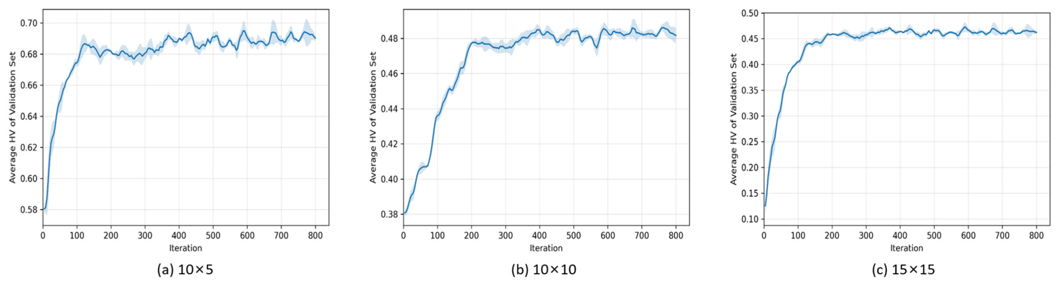
Figure 4, we report the average hypervolume (HV) convergence curves on 100 fixed validation MOFJSP instances for three training scales: 10 × 5, 10 × 10, and 15 × 15. In all three cases, the HV increases rapidly during the early training stage and approaches a stable plateau after approximately 200 iterations, indicating that the proposed method can achieve relatively stable convergence across different training scales.
5.3.1. Results on Training-Scale Synthetic Instances
Table 3 reports the average HV, GAP, and runtime on 100 synthetic test instances at the training scales. Compared with MOEAs that rely on iterative search, DPG-GRL generates Pareto-approximate solution sets with substantially lower inference time while maintaining competitive solution-set quality under the current evaluation setting. As the problem scale increases, the computational cost of MOEAs grows rapidly due to repeated evaluations, whereas the inference cost of DPG-GRL is dominated by a single network forward pass, leading to an even more pronounced advantage at larger scales.
To further assess the statistical reliability of the HV comparisons in
Table 3, two-tailed paired
t-tests were conducted between DPG-GRL and each baseline method over the same test instances, with the significance level set to 0.05. The results show that all pairwise HV differences are statistically significant at the 0.05 level, which further supports the reliability of the observed performance differences.
5.3.2. Cross-Scale Results on Larger Synthetic Instances
To further evaluate cross-scale generalization, we directly test the model trained only on 10 × 10 synthetic instances on three larger settings, namely 20 × 10, 20 × 20, and 30 × 20, without fine-tuning. The results are summarized in
Table 4. DPG-GRL achieves the best HV on all three larger scales, with negative GAP values against all compared MOEA baselines, indicating consistent solution-quality advantages under the adopted evaluation protocol. Although the HV of all methods decreases as the problem scale increases, which is expected due to the higher difficulty of larger instances, DPG-GRL maintains stable relative superiority. In addition, its runtime remains substantially lower than that of the MOEA baselines, and the efficiency gap becomes more pronounced on larger instances. These results indicate that the proposed method exhibits promising cross-scale transfer ability while preserving a clear inference-efficiency advantage.
5.4. Runtime, Complexity, and Scalability Discussion
The runtime results in
Table 3 and
Table 4 show that DPG-GRL consistently requires much less test time than the MOEA baselines, especially at larger scales. This difference is mainly due to the distinct computational structures of the compared methods. Under a trained policy, DPG-GRL generates a solution set by sweeping a fixed set of preference vectors and performing direct policy rollout. Its test-time cost therefore grows primarily with the number of operations, the graph size of the current instance, and the number of preference vectors used at inference. In contrast, the MOEA baselines rely on iterative population search during testing, which involves repeated offspring generation, ranking or decomposition-based update, and repeated objective evaluation. As the problem scale increases, this repeated-search mechanism leads to a much steeper runtime growth than direct policy inference.
It should also be noted that the dual-pool guidance mechanism mainly increases offline training cost rather than inference cost. Specifically, ExpertPool construction, ElitePool maintenance, and replay-based regularization introduce additional overhead during learning, but they do not change the deployed inference procedure once the model has been trained. In this sense, DPG-GRL shifts more computation to the offline stage while preserving a lightweight online decision process. Combined with the results in
Table 3 and
Table 4, this indicates that the proposed method has favorable deployment scalability and is particularly suitable for low-latency scheduling scenarios.
5.5. Comparison with Advanced Baselines
5.5.1. Comparison with the PGRL-Adapted Baseline
To further examine the difference between DPG-GRL and the recent preference-conditioned GRL framework in [
11], we additionally compare our method with the PGRL-adapted baseline defined in
Section 5.2.
Table 5 reports the comparison results on synthetic 10 × 10 instances. As shown, the two methods achieve comparable HV performance, while DPG-GRL requires slightly less inference time. This observation is consistent with the lightweight decoder-level conditioning design adopted in DPG-GRL, which reduces preference-conditioned overhead while preserving competitive Pareto approximation quality.
5.5.2. Results on Public Benchmark Instances
To evaluate solving performance and cross-dataset generalization, we directly apply the model trained only on synthetic 10 × 10 instances to public benchmark instances MK06 (10 × 15), MK08 (20 × 10), La16 (10 × 10), and La21 (15 × 10) without any fine-tuning, and compare it against two advanced baselines, HMOMA and NSGA-III-COE. For each instance, the candidate solution set produced by each method is first filtered to retain only non-dominated solutions, after which HV, GAP, and runtime are computed to evaluate the quality and stability of preference-conditioned solution sets as well as the inference-efficiency advantage of DPG-GRL over iterative-search baselines.
As shown in
Table 6, DPG-GRL achieves competitive solution quality across all public benchmark instances while maintaining a pronounced advantage in computational efficiency. It attains the highest HV on La16 and MK08, outperforming all compared MOEA baselines. On MK06 and La21, its HV remains very close to the best-performing baseline, with gaps of only 0.96% and 0.44%, respectively, indicating stable and high-quality Pareto-front approximation across different benchmark instances. More importantly, compared with iterative-search baselines, DPG-GRL generates solution sets with markedly lower runtime, demonstrating a clear efficiency advantage for low-latency scheduling scenarios.
Overall, despite being trained only on synthetic instances, DPG-GRL maintains reliable performance on public benchmarks without fine-tuning, suggesting promising cross-dataset generalization. Moreover, its low-latency single-model inference makes it well suited for real-time scheduling and industrial scenarios that require fast responses.
5.6. Ablation Study on the Dual-Pool Guidance Mechanism
5.6.1. Mechanism Ablation
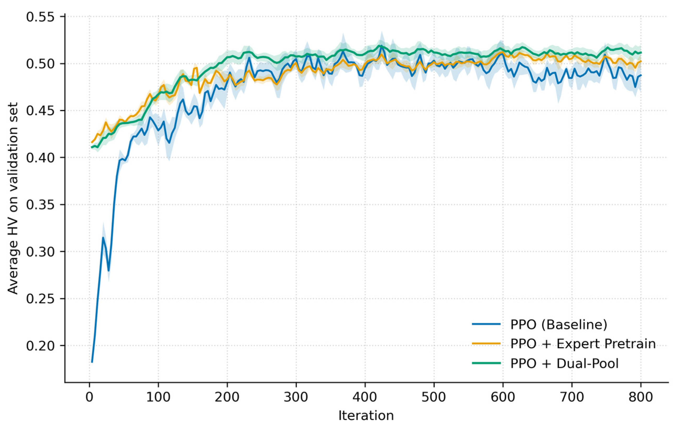
To verify the effectiveness of the dual-pool mechanism, we conduct an ablation study on 10 × 10 synthetic instances by comparing three training settings: PPO (Baseline), PPO + Expert Pretrain, and PPO + Dual-Pool. All settings are evaluated under the same random seeds and identical hyperparameter configurations.
Figure 5 presents the convergence curves of the average HV on the validation set across training iterations.
The results show that expert pretraining substantially increases the initial HV and accelerates convergence to a stable plateau, indicating that offline expert demonstrations provide a stronger behavioral prior and reduce early-stage exploration noise and instability. Building on this initialization, the dual-pool setting further improves the final HV and noticeably reduces mid-to-late training fluctuations, suggesting that the online elite pool continuously feeds back high-quality trajectories and promotes self-improving policy refinement. Overall, the dual-pool mechanism is not a simple additive combination; instead, its two components play complementary roles at different stages of training by improving initialization and enhancing long-term training stability and Pareto approximation quality.
5.6.2. Hyperparameter Sensitivity Analysis
To further justify the choice of BC-related regularization coefficients, we conduct a small-scale sensitivity analysis on the same 10 × 10 synthetic training setting used in the mechanism ablation in
Section 5.6.1. All architectural settings, PPO hyperparameters, and replay-pool sizes are kept unchanged, and only the BC-related coefficients are varied. Results are averaged over three random seeds and reported in terms of Final Test HV and Best Val. HV.
Specifically, we compare four settings: (1) No-BC, where both BC regularizers are removed; (2) Expert-only fixed, where only the offline expert regularizer is retained with a fixed coefficient; (3) Dual-BC fixed, where both offline expert and online elite BC terms are applied with fixed coefficients; and (4) Dual-BC annealed, which is the default setting in the proposed method. This comparison is intended to examine whether BC regularization is beneficial, whether dual-pool BC is preferable to expert-only BC, and whether annealing is more suitable than fixed regularization throughout training. The sensitivity results of the BC-related coefficient settings are summarized in
Table 7.
Removing BC regularization leads to the lowest HV, indicating that pure PPO receives weaker supervised guidance. Introducing the expert BC term improves both Final Test HV and Best Val. HV, confirming the benefit of the offline expert pool as a stable behavioral prior. When the elite BC term is incorporated, performance improves again, suggesting that online self-improving supervision is complementary to offline demonstrations. Among the tested settings, the annealed dual-BC scheme achieves the best performance, indicating that strong early guidance followed by gradual relaxation is more effective than maintaining fixed BC strength throughout training.
6. Conclusions
This paper proposes an end-to-end method for MOFJSP, referred to as DPG-GRL. The proposed approach integrates a graph attention network with reinforcement learning, models operation–machine coupling via a heterogeneous graph representation, and explicitly injects a preference vector into the policy network. As a result, the trained model can rapidly generate Pareto-approximate solution sets under different preference vectors at inference time, thereby covering diverse trade-offs among multiple objectives. To improve sample efficiency and training stability, we further introduced a dual-pool guidance mechanism: offline expert demonstrations provide stable early-stage guidance, while an online elite pool continuously feeds back high-quality trajectories to enhance policy stability and solution-set quality. Experimental results show that DPG-GRL achieves competitive performance on both synthetic instances and public benchmarks in terms of HV and GAP, while being significantly faster during inference than MOEAs that require iterative search. These results indicate promising generalization to unseen instances and practical potential for low-latency scheduling applications.
Despite these encouraging results, several limitations of the present study should also be acknowledged. First, the preference decomposition relies on weighted-sum scalarization, which may provide limited coverage for non-convex regions of the Pareto front. Second, although the dual-pool mechanism empirically improves sample efficiency and training stability, a more rigorous theoretical convergence analysis of the regularized PPO framework remains a valuable direction for future research. Third, the present study is confined to the static MOFJSP setting, and dynamic disruptions such as machine failures or unexpected job arrivals are beyond the scope of the current work. Finally, validation on proprietary industrial datasets or real production scenarios is still needed to further assess practical applicability. Future work will investigate alternative scalarization schemes, alternative reward-shaping strategies, dynamic scheduling extensions, more realistic due-date and energy models, and broader validation in industrial scenarios.