Using an Accelerometer for State Estimation on an Icosahedral Tensegrity Structure

Abstract

This paper presents a methodology for implementing a Kalman filter on an icosahedral tensegrity system capable of performing state estimation on an icosahedral structure. A motion model based on the geometry of the system and a measurement model based on the Inertial Measurement Unit (IMU) data are derived for this purpose. Due to the nature of icosahedral tensegrity robots, accurately predicting the state of the robot through conventional models is difficult, primarily because the entire structure is rotated in 3D space during movement. As such, adding bearing or distance sensors to this robot is very difficult, since the location of those sensors with respect to the base frame changes with every rotation. This paper instead uses a simple kinematic model based on the predicted geometry of the structure to act as the motion model and uses the data from an accelerometer to create a measurement model. These models are then used in a Kalman filter to estimate the state of the system.

1. Introduction

This paper utilizes the data from an IMU and the geometry of an icosahedron to perform state estimation on an icosahedral system from an initial state. This state comprises the planar x-y coordinates of the system, as well as a quaternion that represents the rotation of the system. That information is then combined within a Kalman filter, where the motion model is based on icosahedral geometry and the measurement model is constructed utilizing data acquired from an IMU. The Kalman filter is updated iteratively with the movement of the system.

State estimation has two parts. The first part of state estimation is the motion model. This model will predict how the system moves between rotation events, showing the change in global x-y displacements and system rotation. The motion model has uncertainty because the physical system is not a perfect icosahedron, the exact geometry is not known, and the system could slip when movement occurs. The second part of state estimation is the measurement model, which is derived from IMU readings recorded during the motion event. The data collected from the IMU can be used to estimate the motion of the system. That estimate can be combined with the estimate from the motion model to reduce the uncertainty of the system state.

This paper shows a novel motion model specifically designed for an icosahedral structure. In addition, it demonstrates the application of Kalman filtering techniques to an icosahedral tensegrity structure by leveraging IMU measurements and geometric constraints to reliably estimate the state of the system. The novelty of this approach revolves around having a motion model that works very well even with problematic measurements.

The structure of the paper is organized as follows: first, an overview of relevant background information is given, setting the stage for understanding the motivation behind addressing this specific problem. Next, the methodology for determining the support polygon and the rotation matrix is given. The motion model and the measurement model of the system are then described. The motion and measurement model are then combined together into a Kalman filter and the results are shown.

IMUs have been used for state estimation for a variety of different applications [1]. These systems include using an accelerometer for state estimation in soft robotics [2,3], and other traditional forms of rigid robotics as well [4]. In these applications, accurate estimates of the current state of the system were needed to successfully manipulate the trajectory.

To fully know the orientation of a system, it is necessary to estimate the system’s quaternion, often estimated through a Kalman filter [5,6,7,8]. This approach is implemented on a wide range of applications, such as helicopters [9], quadcopters [10], underwater navigation [11], and other robotic applications [12]. With a quaternion, it is possible to precisely identify which nodes comprise the polygonal support of the system.

State estimation is often used when localizing a system [13]. These state estimation techniques typically rely on knowledge about the motion of the robot, as well as some kind of measurement to predict where the robot is located. The motion and measurement information are then combined in what is commonly referred to as a filter. These filters are often particle filters [14,15], or some rendition of a Kalman filter [16,17,18], both of which have unique advantages and disadvantages.

Tensegrity structures have been analyzed and used in many different fields, from structures [19] to robotic manipulators [20], and from morphing wings [21] to robots capable of locomotion [22]. One common structure used in tensegrity robotics is an icosahedron (20-face polyhedron). Motion has been created in this structure through a variety of different methods, including hopping [13], variable mass bars [23,24,25] and varying string length [26]. All these implementations have yet to address the unique state estimation problem in tensegrity robots. Since all these structures rotate between states, an algorithm needs to be created to estimate the state of these structures. Icosahedral shapes are also used in robotics outside of tensegrity [27], allowing for this method to be relevant even outside of the tensegrity field.

State estimation on tensegrity structures has been attempted [28,29,30], with additional emphasis on other forms of pose tracking [31,32,33]. These efforts focused on fusing several types of sensors into a single Kalman filter. This work on the other hand creates a novel, simplified motion model from the geometry of the structure. Specifically, the motion model considers that propagation of uncertainty occurs only when the robot is rolling, and that uncertainty is more likely to propagate in the direction of the momentum of the robot during the roll compared to other directions. Estimation efforts have also occurred on robots that have similar properties to tensegrity robots, such as soft robots [33] and spherical robots [34,35,36,37]. Due to the quasi-static nature of the motion, rotational state information is computed directly from geometric constraints and used to transform measurements prior to filtering, allowing the use of a linear Kalman filter for state estimation.

2. Materials and Methods

2.1. Support Polygon for Icosahedral System

An icosahedral tensegrity system has 20 faces, 6 bars, and 24 cables. All pertinent lengths can be derived from the length of the bars. For this work, the bar length was chosen to be 600 mm, which gives a cable length of 367 mm. Each face is defined by three unique points, where each point is a vertex of a regular icosahedron. Therefore, the current support polygon can be defined as the three vertices closest to the ground, assuming a flat ground. 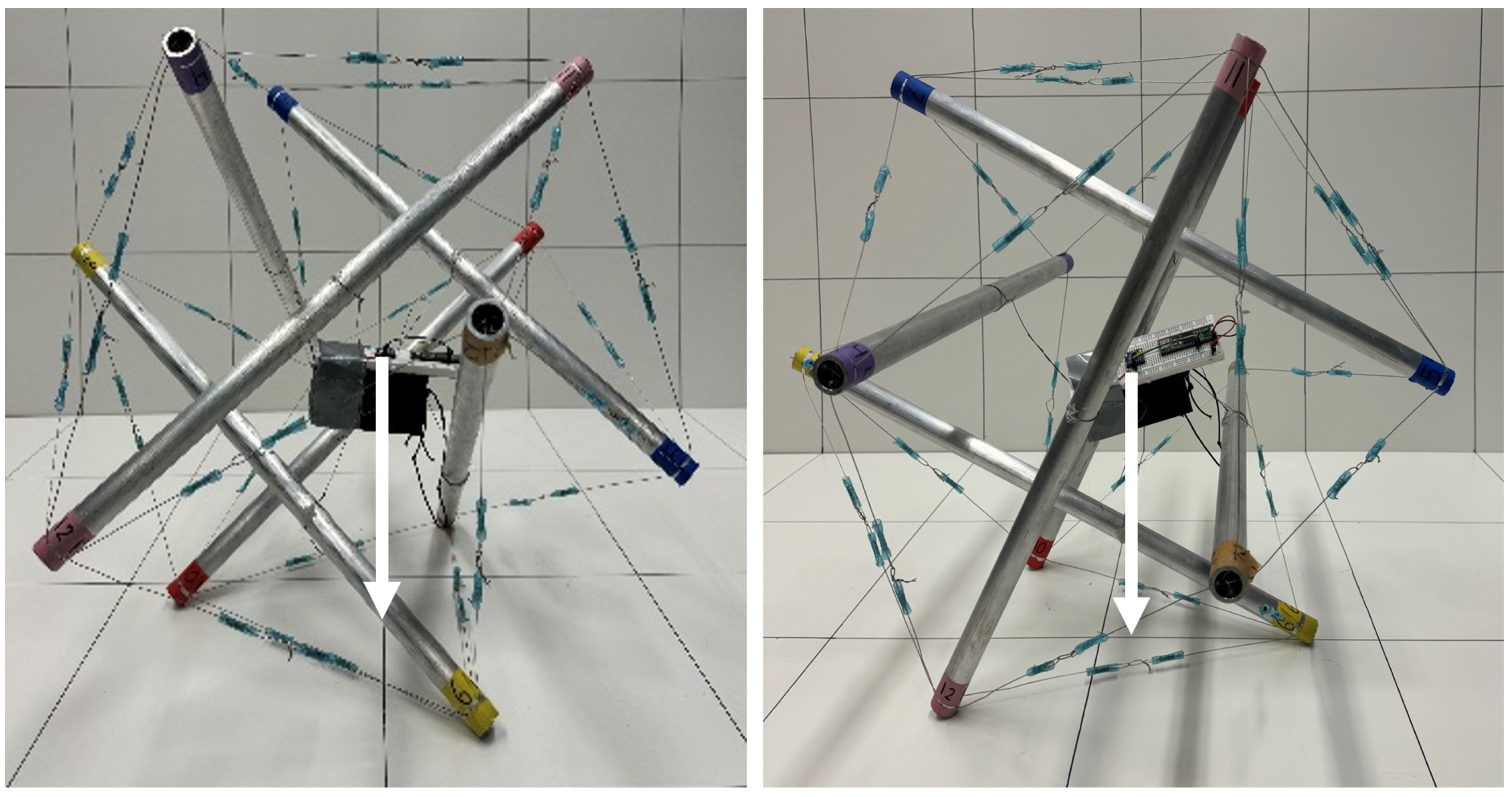Figure 1 shows an icosahedral tensegrity structure in two different orientations. If a 3-axis accelerometer is fixed to the robot, in a static configuration the accelerometer readings will point to the base that is on the ground. These readings are shown as an arrow in Figure 1. For this method to work, the sensor frame and the system frame begin in the same orientation. In addition, the system frame is located at the center of the system, with the z axis pointing up.

Once the system is properly oriented, identifying the support polygon is accomplished by calculating the dot product between the accelerometer’s reading and each vertex’s vector. The white arrow represents the acceleration vector recorded by the accelerometer, showing the direction of gravity. These vectors are defined by the positional vector extending from the structure’s center to the node at the end of each bar. Subsequently, the three with the highest dot product values are selected. This method is effective since the accelerometer’s readings are best aligned with the vertices forming the face towards which it is oriented. This method can work on any tensegrity structure if each node can be defined from the center of the structure.

2.2. Rotation Matrix Methodology

To determine the rotation matrix, the first step is to know the location of three ground nodes from the initial orientation of the object. These are the three initial points used in calculating the rotation matrix. Each of these points have an x, y, and z component, thus when appended together it creates the matrix:

$$\left[\begin{array}{ccc}{n}_{1i}& n_{2i}& n_{3i}\end{array}\right]=N_i$$

(1)

where $n_{1i}, n_{2i}, \mathrm{a}\mathrm{n}\mathrm{d} n_{3i}$ are the coordinates of the three nodes that represent the initial system state. The same process is applied to the nodes after the system has rotated:

$$\left[n_{1f}, n_{2f}, n_{3f}\right]=N_f$$

(2)

where $n_{1f}, n_{2f}, \mathrm{a}\mathrm{n}\mathrm{d} n_{3f}$ are the coordinates of the three nodes that represent the final system state.

Using the definition of a rotation matrix, the following can be determined:

$$N_f=R{N}_i$$

(3)

Solving for R yields

$$N_f{N}_i^{-1}=R$$

(4)

The initial nodes of this system are the location of the nodes at the current time step. These locations are calculated by multiplying the current rotation matrix by the first locations of the nodes. The final nodes are the projected location of the nodes at the next time step. The projection is determined by taking the location for the two nodes about which rotation happened and estimating the position of the third base node. To calculate the location of the third node of the system, it is assumed the node will be located at the average height of the other two nodes, translated perpendicular to the center of the rotation vector by

$${\displaystyle \frac{\sqrt{3}}{2}}\ast s$$

(5)

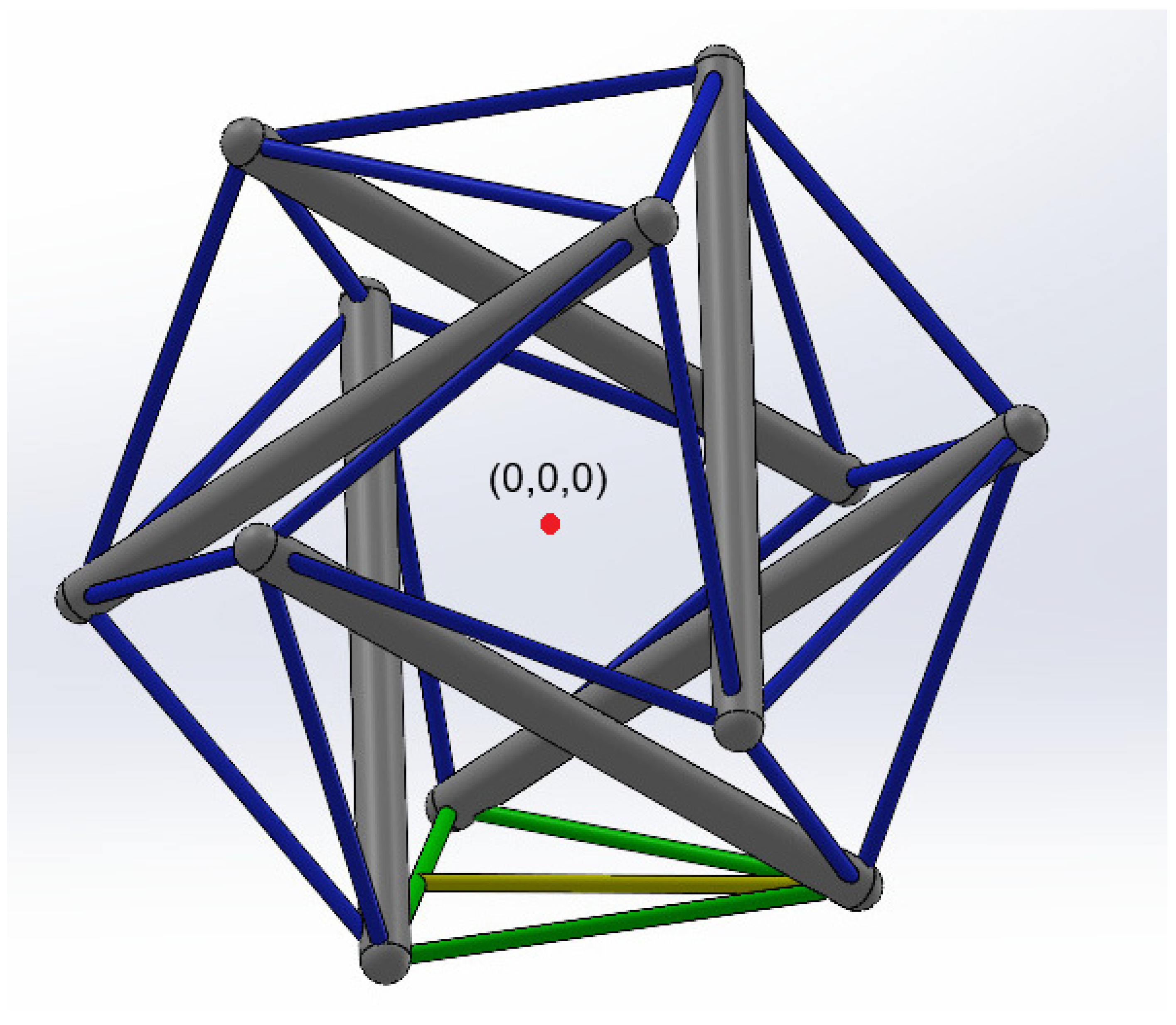
where s is the length of one of the edges. The initial nodes and the final nodes are then translated so that the system’s centroid is at (0,0,0), as illustrated in Figure 2.

Now that $N_i$ and $N_f$ are determined, R can be solved for with Equation (4). To get the entire rotation of the system up to the point $N_f$, multiply the previous rotation matrix by the newly acquired rotation matrix. The rotation matrix that describes the final rotation is converted to a quaternion so it can be represented as part of the state.

2.3. Tensegrity Motion Model

To predict the motion of the icosahedral structure, the geometry of the icosahedron is heavily leveraged. A regular icosahedron is composed of congruent equilateral triangles. The height of the triangle, as shown in Figure 2, is twice the x-y distance that the structure moves each time it rotates, which will be either 319 mm or 335 mm, depending on the face.

With the distance caused by rotation known, the last thing to determine is the direction of movement. To do this, the current orientation of the structure must be known. As the structure rotates, the total rotation of the structure is updated using the method discussed previously. Rotating the initial state by the total rotation gives the orientation of the structure. The orientation then reveals the directions the structure can move.

At each time step, the base of the structure is reevaluated. If the structure ‘s base has changed, then rotation has occurred. The new base nodes of the structure are determined, the new base is compared with the previous base, and the nodes that are the same between the two bases are selected. The difference between those nodes is the vector about which rotation occurs. A vector perpendicular to the rotation vector is the direction in which movement occurred. The direction vector must be in the direction of movement and is created as a unit vector.

The movement of the model is estimated by multiplying the distance vector by Equation (5). The estimated state is then augmented by that value. The state estimate is the location of the robot’s center of mass and a quaternion representation of the rotation of the model. When the model is initialized, this x-y state is set to (0,0) and the quaternion is initialized to (1,0,0,0).

To represent the covariance in a way that is consistent with a discretized state space model, the covariance is preserved at each timestep, with two additional uncertainties added to it: uncertainty due to geometry, and uncertainty due to the momentum of the structure.

2.4. Measurement Model

To create the measurement model of this system, the data from an IMU was used to determine the current predicted state of the structure. The MPU6050 library by ElectronicCats was used to extract the information needed for the measurement model.

Due to the quasi-static nature of this problem, the measurements taken during each measurement interval were combined until the motion model was reevaluated. To combine the data, the sensor data was transformed into acceleration and integrated using

$$x_t={\displaystyle \frac{1}{2}}{a}_t{t}^2+v_{t-1}t+x_{t-1}$$

(6)

where $a_t$ is the acceleration received by the accelerometer at the current time step $v_{t-1}$ is the velocity of the previous time step and $x_{t-1}$ is the previous position. The velocity and position are updated iteratively. It is important to note that dead-reckoning caused by this model is mitigated by filtering low acceleration and only using the measurements if the structure has moved. If needed, the process can be further improved by providing stationary periods where the system is known to be still and the accelerometer can be recalibrated.

For the approach described in Equation (6) to work, it is essential that the acceleration vector is aligned with the world frame. Given that the structure may undergo rotation at each time step, the accelerometer data must be rotated into the world frame. This adjustment involves analytically rotating the accelerometer to align with the structure’s rotation and subtracting the gravity component to isolate the structure’s movement.

This adjustment is achieved by incorporating a gyroscope capable of deriving a quaternion prediction at each structure state. The quaternion is derived from the gyroscope by integrating the gyroscope’s values over time. This quaternion is used to rotate the accelerometer into the base frame and remove gravity. The quaternion is used as the rotation measurement for the structure. The IMU is fixed in position at the center of mass of the system through a set of 4 taut wires, which was sufficient for accurate results on the quasi-static system.

Two distinct update rates are used in this implementation. The inertial measurement unit (IMU) is sampled at a relatively high frequency (on the order of 10–100 Hz), while state updates within the Kalman filter occur at a much slower rate, corresponding to the completion of a discrete rotation event. This slower update rate is typically on the order of several seconds and reflects the quasi-static nature of the system’s motion.

Bias handling for the IMU was intentionally simple for this iteration of the system. No explicit bias estimation or correction was performed. Instead, accelerometer measurements were discarded during periods when state updates were not required. While this approach limits long-term accuracy, it was sufficient for demonstrating the effectiveness of the geometry-based motion model and is identified as an area for improvement in future work.

Stationarity of the system is inferred from geometric information rather than signal-level detection. When the support polygon is observed to change, the system is assumed to have completed a rotation and to be resting flat on the newly identified base. During these intervals, the system is treated as quasi-static.

All inertial measurements are first transformed into the body frame using the externally computed quaternion derived from the system geometry. Gravity is then removed from the transformed acceleration vector to isolate translational motion prior to integration.

The order of operations for inertial processing is therefore: (1) computation of orientation from geometric constraints, (2) transformation of accelerometer data into the body frame, (3) gravity subtraction, and (4) integration of the remaining acceleration during motion intervals.

The combination of the position and the quaternion estimates compose the measurement model of the structure and can be used in a Kalman filter to improve the estimated state of the structure. Integration errors arising from accelerometer drift are not explicitly eliminated in this iteration of the system. Instead, the geometry-based motion model provides the primary source of displacement estimation, with inertial integration contributing supplementary information during motion intervals. This limitation is acknowledged, and future work will focus on incorporating absolute references to reduce reliance on dead-reckoning.

2.5. Kalman Filter Implementation

Although the system undergoes three-dimensional rotation, the Kalman filter implemented in this work does not explicitly propagate nonlinear rotational dynamics. Due to the quasi-static nature of the motion, the orientation of the structure at each timestep is computed externally using the geometry of the icosahedral support polygons. This orientation, represented as a quaternion, is used only to transform inertial measurements into the world frame prior to entering the Kalman filter. As a result, the filter operates on pre-processed state estimates rather than directly modeling quaternion kinematics, allowing a standard linear Kalman filter formulation to be used.

$$x[k+1]=Ax\left[k\right]+Bu\left[k\right]$$

(7)

$$y\left[k\right]=Cx\left[k\right]+Du\left[k\right]$$

(8)

This paper assumes that actuating the system causes all changes to $x[k+1]$. As such, A is the identity. B was estimated by using the motion model process. It is also assumed that the output is the observed states, so C is an identity matrix, while D is the 0 matrix, as no direct feedthrough exists.

Because the filter does not estimate or propagate quaternion state derivatives, unit-norm constraints and nonlinear quaternion update equations are enforced outside the filtering framework. At each polling interval, the quaternion is recomputed from geometric relationships and renormalized before being used for measurement transformation. Consequently, no nonlinear rotational state evolution occurs within the Kalman filter itself.

Uncertainty from the motion model and from momentum sliding is added at each time step. The variance in state due to the motion model in the x-y direction was approximated as 2 cm and from the momentum sliding was 4 cm. From simple testing, these values were deemed appropriate. A large value was used for the rotation uncertainty from the motion model. The process noise covariance values were selected empirically based on repeated experimental observation of slip magnitude and rotational variability during rolling. Rather than representing sensor noise alone, these values capture unmodeled effects such as contact uncertainty, geometric imperfections, and minor sliding during rotation. While these parameters are not optimized statistically, they were found to provide consistent and stable estimation performance across the tested trajectories. While the injected process noise is modeled as independent in each state component, correlations between states naturally arise through the prediction and update steps of the Kalman filter. The independence assumption applies only to the uncertainty added at each timestep and reflects the physical interpretation of the dominant error sources.

The state vector tracked by the Kalman filter consists of planar position and orientation, (x,y,θ). Process uncertainty is injected at each timestep to account for geometric imperfections and potential slip during rolling. This injected uncertainty is modeled as independent in each state component, reflecting the physical interpretation that translational slip in the x-direction primarily affects x, slip in the y-direction primarily affects y, and rotational uncertainty affects θ. While cross-correlations between states naturally arise through repeated prediction and update cycles, the uncertainty added at each step is assumed independent to reflect the underlying error sources.

3. Results

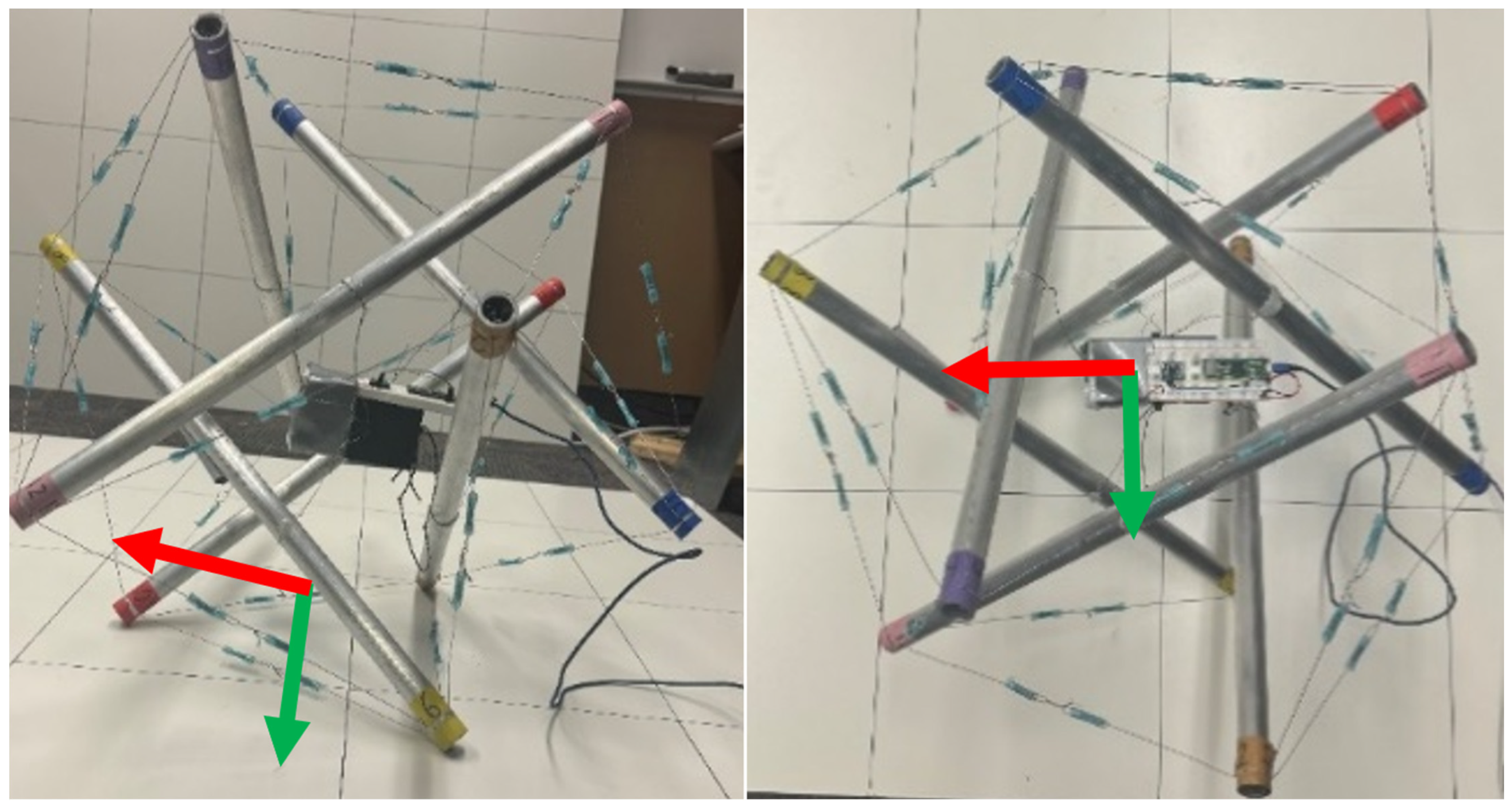
To test the filter described above, we started by creating an icosahedral system, as shown in Figure 3, that has an accelerometer rigidly attached to the system, located near the centroid of the system. This accelerometer sends data to an Arduino running the Kalman filter for processing.

The IMU was mounted near the center of mass of the structure using a set of taut cables. While this mounting approach introduces potential sources of error such as eccentricity, compliance, and vibration, the quasi-static operating conditions of the system limited these effects in practice. This method was chosen to minimize interference with the structure’s motion while maintaining sufficient measurement fidelity. The influence of sensor mounting and structural dynamics represents an additional source of uncertainty and will be addressed in future iterations through improved mounting strategies.

Using that data, the base of the system at each time step was calculated. By following the procedure outlined previously, the system could go from an arbitrary face to any other face, and the accelerometer method would correctly identify the base every time.

When the structure was initialized, the initial rotation matrix was set to the identity matrix. Then, the system was rotated to a new face, and the new matrix was checked to ensure that it is part of the Special Euclidean group. The criterion for validating the rotation matrix involves verifying that the determinant of the rotation matrix equals 1. Once the structure parameters were properly tuned from observed patterns, testing showed that the determinant from one rotation to the next were between 0.99 and 1.01. This was renormalized at every time step. The gain for the system was determined based on the slip deviation that was calculated.

To verify that the rotation matrix was determined correctly, the system was rotated through a series of steps, and then followed the reverse of that path back to the original position. Such a procedure should ideally lead the motion model to predict an identity matrix for the rotation matrix in the final state. The outcome of this experimental test yielded an approximation of the identity matrix, indicating the rotation matrix’s effectiveness in modeling the system’s orientation accurately. A variant of this test was conducted where the system ended up its same initial face, but with some rotation about the global z axis, and the predicted matrix still closely aligned with the expected outcomes, demonstrating the robustness of rotation matrix calculation.

To further validate the x-y component of the motion model, the system was subjected to various path trajectories to assess the performance of the system. It is important to emphasize that this type of testing also serves as an evaluation of the rotation matrix of the system as well, since reasonable x-y values depend on a good approximation of the rotation matrix.

The experiment design was as follows:

1.

The robot was placed on a grid at a location defined as (0,0). In addition, the robot was placed in a predefined orientation, with the same starting base as well as the three base nodes located in the same location. That location was determined by marking the location of where each node must start on the measurement grid.

2.

The person performing the test rotated the robot about one of the three edges of the base, attempting to ensure that the robot pivoted without slipping.

3.

The tester waited for a state update to appear in the terminal, signaling that the algorithm detected a new orientation and has a new prediction for the current state of the system. The delay in the system was set by the tester to match the speed at which they wanted to test.

4.

The process above repeated until the robot reached the final desired location.

All experiments were conducted in a controlled laboratory environment on a uniform, flat surface. No data were collected on alternative terrains due to operational constraints. As such, the reported results reflect performance under consistent surface conditions, and performance on varying terrain remains an open area for future investigation.

Direction and reproducibility were ensured by ensuring the same start state by denoting starting orientation and position. Ground truth was determined by performing the test on a known grid. At each step, the location of the center of the robot was measured and recorded. This ground truth was the result of real-world events such as slip and incongruent faces. The result from the motion model with state estimation was compared to an estimate using only acceleration data. However, due to the highly flexible structure, significant sensor uncertainties, and the inherent challenges of integrating acceleration to determine displacement, the estimates derived from acceleration data alone were unusable. In fact, errors for each rotation were often larger than the maximum expected travel distance for each roll. This result does demonstrate the effectiveness of the motion model, which does not rely solely on acceleration data and is able to provide meaningful state estimates where direct accelerometer integration fails.

Once the motion model has been successfully validated, the next critical step is to validate the Kalman filter itself. This involves ensuring that the filter accurately integrates incoming data, effectively estimates the system’s state, and adjusts its predictions based on the observed measurements. This validation process is essential for confirming the Kalman filter’s efficacy in real-time data assimilation and its capability to provide precise state estimations under varying conditions. The validation strategy for the Kalman filter consisted of several trials of 5 unique trajectories and 2 extended trajectories. The results are summarized in

Table 1. The result from each trajectory is summarized here. The degrees refer to the angle from the y axis that the system moved along, where 0 degrees is along the y axis. Note that the distance traveled is different for each trial and that stationary data was removed.

	0 Degrees	25 Degrees	45 Degrees	−25 Degrees	−45 Degrees
Mean Distance from Target: (m)	0.167	0.235	0.128	0.186	0.195
Standard Deviation:	0.17	0.32	0.13	0.18	0.52
Error as Percentage of Distance:	9.2%	11.6%	5.0%	9.1%	7.5%

. Each trajectory presented in this table (0 degrees, 25 degrees, etc.) was repeated five times in order to calculate basic statistics.

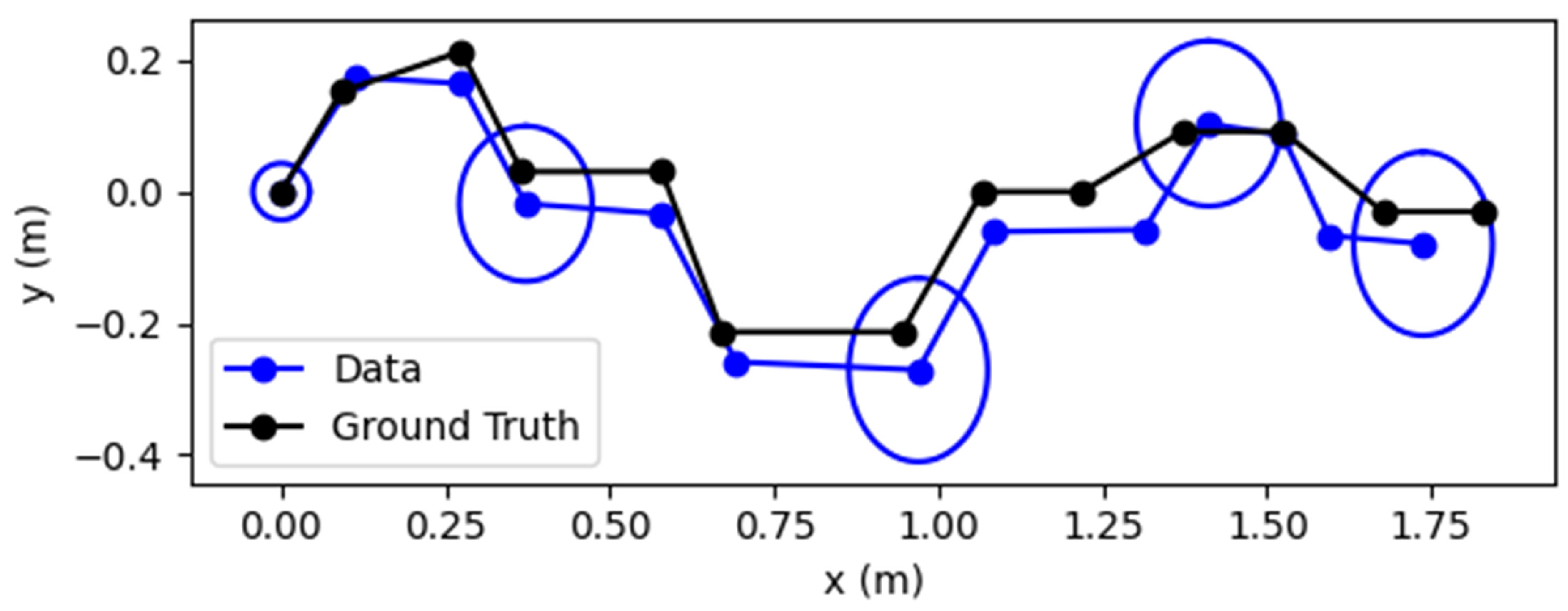
The results of the extended trajectories matched the same percentage of error for the distance traveled. The covariance growth observed along the direction of travel reflects the accumulation of uncertainty over successive rotation events, while the narrower covariance perpendicular to motion is consistent with the anisotropic uncertainty model used in the filter. The covariance of the system following the 0-degree trajectory shown in Table 1 is shown in Figure 4. The observed error reflects the cumulative effect of multiple discrete rotations. As the number of steps increases, small errors in rotation estimation, slip during contact, and geometric imperfections accumulate, leading to increased positional deviation. This behavior is consistent with the quasi-static rolling nature of the system.

The relatively larger standard deviations observed for certain directions are primarily attributed to sensitivity to initial orientation, variations in friction during rotation, and small inconsistencies in how the structure contacts the ground between steps. Additionally, minor deviations in the estimated rotation matrix can compound over successive steps, contributing to directional variance.

4. Conclusions

This study demonstrates the application of a Kalman filter to an icosahedral tensegrity system for estimating the state of the system from an initial state. Utilizing data from an IMU and leveraging the known geometry of the icosahedron, the filter achieved reliable position estimation.

By adapting this approach, the principles of both the motion and measurement model can be extended to cable driven tensegrity systems provided the nodes’ locations within the system are known. The use of a Kalman filter could help to better predict the current system’s pose.

Most inaccuracies within the measurement model were observed in the x and y coordinates, attributable to the double integration performed on the acceleration data. To mitigate these errors in future iterations, implementing a low pass filter on the acceleration data is recommended. This adjustment is expected to refine the signal quality by attenuating high-frequency noise, thereby enhancing the precision of the integration process and reducing overall measurement discrepancies.

Overall, this work demonstrated the capability to estimate the state of a nonlinear icosahedral tensegrity system using a Kalman filter. It developed a motion and measurement model that relies on the geometry of the model IMU data. This paper shows how IMU data can be used to determine the pose of the system as the system moves. The simplicity of this model is also important. The entire program can run on a microcontroller, allowing for fewer resources to be dedicated for state estimation.

While this work focuses on a specific icosahedral tensegrity structure operating under quasi-static conditions, the underlying principles of geometry-based motion modeling and inertial data fusion are applicable to other rolling polyhedral and tensegrity systems. Future extensions will investigate the use of absolute landmarks, such as visual features detected by onboard cameras, to further reduce integration drift and improve robustness in more dynamic environments. Future work will focus on increasing the number of trials, evaluating performance on varied terrain, and analyzing error growth as a function of step count to further characterize the robustness of the approach.