Physics-Informed Bayesian Inference for Virtual Testing and Prediction of Train Performance

Abstract

This paper proposes a physics-informed Bayesian framework for virtual testing and predictive modeling of train performance, specifically addressing stopping-distance prediction. The approach unifies physical simulation models with data-driven statistical inference to achieve uncertainty-aware predictions under limited or noisy measurements. By embedding governing equations of motion into a hierarchical Bayesian structure, the method systematically accounts for both model-form and data uncertainty, allowing explicit decomposition into aleatoric and epistemic components. A Gaussian process surrogate is employed to efficiently emulate high-fidelity physics simulations while preserving key dynamic behaviors and parameter sensitivities. The Bayesian formulation enables probabilistic calibration and validation, providing predictive distributions and confidence bounds. As a representative application, the framework is applied to the virtual prediction of train stopping distances, demonstrating how the proposed methodology captures nonlinear braking dynamics and quantifies uncertainty in safety-relevant performance metrics directly compatible with statistical verification standards such as EN 16834. The results confirm that the physics-informed Bayesian approach enables accurate, interpretable, and standards-aligned virtual testing across a wide range of dynamical systems.

1. Introduction

Virtual testing is rapidly transforming safety-critical engineering by enabling performance evaluation through computational simulation, reducing reliance on full-scale, costly experimental campaigns. This approach leverages advanced computational models to predict system behavior under a range of operating conditions, accelerating design, certification, and operational decision-making. At the core of this methodology, physics-informed modeling explicitly incorporates governing physical laws such as conservation of energy and momentum, constitutive material behavior, and thermal transfer into the computational framework. By embedding these principles, the hypothesis space is constrained to physically admissible trajectories and material responses, which reduces data requirements, mitigates overfitting, and improves extrapolation to conditions underrepresented in experimental measurements [1,2].

In parallel, Bayesian inference provides a principled probabilistic framework to represent uncertainties arising from unknown model parameters, measurement noise, and potential model discrepancy. By updating prior beliefs with observed data, Bayesian methods generate posterior distributions that quantify both epistemic and aleatoric uncertainty, rather than producing a single deterministic prediction [3,4]. Modern computational approaches including Hamiltonian Monte Carlo, variational inference, and ensemble Kalman inversion enable tractable inference for high-dimensional, nonlinear systems, facilitating the integration of physics-based priors with sparse or noisy observational data. The synergy of physics-informed modeling and Bayesian inference thus allows for predictive simulations that are not only consistent with fundamental physical laws but also accompanied by well-characterized uncertainty metrics.

The utility of such a framework becomes particularly evident in domains where full-scale experimental evaluation is challenging, costly, or risky. Rail vehicle braking provides a prototypical example. Braking performance is governed by complex, coupled interactions between vehicle dynamics, frictional contact at the wheel–rail interface, brake pad and disc thermomechanics, and environmental factors. Regulatory standards, such as EN 16834 and the EN 14531 series, specify procedures for validating brake performance through stopping distance measurements, deceleration profiles, and braked weight evaluation [5,6]. While these standards provide deterministic calculation methods and statistical validation criteria (e.g., K1 and K2 for stopping distance uncertainty), they do not explicitly incorporate probabilistic uncertainty arising from operational variability, measurement errors, or frictional stochasticity. Physics-informed Bayesian virtual testing addresses this gap by predicting performance metrics under a range of operational scenarios while providing confidence intervals and risk estimates, effectively complementing existing standards [7,8,9,10].

Over the past decades, computational frameworks for brake performance have evolved significantly. Early deterministic analytical methods estimated stopping distances based on mean-value analyses [11,12], while later efforts incorporated variable loading conditions, thermal effects, and frictional dynamics in iterative simulation tools [13,14,15,16]. More recent approaches have introduced mathematical models capturing critical parameters such as braking force, train resistance, wheel–rail adhesion coefficients, and transient pressure dynamics in brake cylinders [17,18]. However, most existing models remain deterministic, limiting their ability to quantify uncertainty and assess risk. Monte Carlo simulations and other stochastic approaches have partially addressed this limitation [8,9,10], but a unified framework systematically integrating physics-based modeling, Bayesian inference, and probabilistic virtual testing is still lacking.

A physics-informed Bayesian approach offers a structured solution. By combining mechanistic priors derived from physical principles with observed data, the posterior model can iteratively refine predictions of system behavior while naturally capturing uncertainty from all relevant sources. Surrogate models, such as Gaussian Processes, provide flexible, nonparametric representations of nonlinear dynamics and allow the propagation of uncertainty into critical output quantities, such as stopping distances and deceleration rates. These probabilistic predictions are directly interpretable within regulatory contexts, facilitating risk-informed decision-making and compliance with standards like EN 16834 [5,6].

Virtual testing enabled by this framework supports a coherent workflow: first, developing a physics-informed model capturing essential system dynamics; second, calibrating the model with available experimental or field data; third, performing posterior predictive simulations under representative operational scenarios; and finally, quantifying the probability of meeting or violating performance criteria. While railway braking serves as a concrete example, the framework is generalizable to other safety-critical systems where experimental campaigns are expensive, operational variability is high, and reliable predictions under uncertainty are essential. In this sense, the railway application highlights both the potential impact and practical relevance of physics-informed Bayesian virtual testing, without limiting the framework’s applicability.

Two major challenges arise in the development of a probabilistic framework for virtual prediction. First, the nonlinear behavior of dynamics under varying conditions complicates the accurate modeling of the relationship between predictors and output. Second, the availability of limited experimental data poses difficulties in reliably quantifying uncertainties. Bayesian inference offers a principled solution by enabling the integration of prior domain knowledge, often derived from physics-based simulations, with sparse observational data. This is particularly valuable when experimental data is limited or costly to acquire. When combined with Gaussian Process (GP) regression, the approach provides a flexible, non-parametric means of capturing complex input–output relationships while naturally quantifying predictive uncertainty. The GP serves as an effective surrogate model, not only representing nonlinear dynamics but also producing confidence intervals that are directly interpretable within the context of statistical validation frameworks such as EN 16834. This synergy enhances predictive accuracy and supports adaptive learning from limited or noisy data, thereby facilitating compliance with regulatory requirements.

The proposed probabilistic framework integrates deterministic modeling with Bayesian inference and Gaussian Process (GP) regression to enable uncertainty-aware predictions. A physics-based simulation model of the problem under study is first employed. This surrogate model is then used as the prior mean function within the GP framework, thereby embedding physical knowledge into the probabilistic prediction process. To account for real-world variability and potential model inaccuracies, the parameters of the deterministic surrogate are treated as uncertain quantities and updated through a Bayesian calibration procedure. Experimental test data, serving as training data, is used to refine the prior distributions of these parameters, resulting in an updated posterior mean function that better aligns with observed behavior.

In addition to the mean function, the GP formulation requires a prior covariance function that encodes assumptions about the smoothness and correlation structure of the input–output relationship. A radial basis function (RBF) kernel is adopted for this purpose, and its hyperparameters, governing the length scale and signal variance, are also inferred from the calibration data using Bayesian updating. This allows the model to adaptively learn the functional behavior directly from observations.

By updating both the mean and covariance functions using training data, the framework yields a posterior GP model that provides probabilistic predictions of stopping distances at new, unseen test (validation) points. These predictions include not only point estimates but also confidence intervals that reflect uncertainties in estimation of the stopping distance. The resulting approach ensures a strong physical foundation while maintaining the flexibility to incorporate empirical evidence, supporting reliable and regulation-aligned virtual testing in accordance with standards such as EN 16834.

Classical braking-distance studies use deterministic models with Monte Carlo perturbations to represent variability, which quantifies spread but does not reconcile model-form discrepancy with test data in a unified Bayesian update. Purely data-driven Gaussian Processes improve interpolation but risk unrealistic extrapolation and lack physical interpretability, while physics-informed neural approaches (e.g., PINNs) primarily target inverse problems rather than regulatory validation workflows. The present framework embeds a validated brake simulator as the GP mean to enable test-driven Bayesian calibration of both mean and covariance, models heteroskedastic noise by velocity groups aligned with EN 16834 sampling, and reports K1/K2 statistics from the posterior predictive distribution as standards-aligned evidence, an incremental methodology tailored to certification-adjacent railway practice. The work employs a physics-based brake model for providing the prior mean of stopping distance as a function of initial speed; a Gaussian-process discrepancy, calibrated to measured track tests, yields the posterior predictive distribution in lieu of a point estimate. The associated credible intervals reflect both aleatoric variability (measurement scatter) and epistemic uncertainty (model-form simplifications and limited data) and are evaluated against EN 16834 K1/K2 thresholds for standards-aligned assessment.

The structure of this paper is as follows: Section 2 presents a deterministic surrogate model for stopping distance prediction. Section 3 motivates the need for a probabilistic framework to quantify uncertainty, outlining key methodologies and their application to stopping distance estimation. The validation of the proposed framework through case studies and comparative analyses are provided in Section 4. Finally, Section 5 summarizes the main findings and outlines directions for future research.

2. Physics-Informed Mathematical Model

As a practical application, we explored the use of the method in railway engineering, focusing specifically on virtual testing of brake system performance. For this purpose, the underlying mathematical model capturing the relevant physical phenomena is introduced in this section. In such a framework, the brake pad, disc, and vehicle are treated as coupled subsystems whose behavior evolves simultaneously during a braking event. As mechanical power is dissipated at the friction interface, part of it is transformed into heat within the pad–disc pair, causing their temperatures to rise. Heat is then redistributed between pad and disc through thermal conduction, while convective exchange with the surrounding airflow contributes to energy loss. At the same time, the frictional force opposes motion, reducing vehicle speed. This formulation results in a thermomechanically coupled model that has become standard in brake thermal analyses [19], offering a physically grounded means of predicting both thermal response and deceleration under varying operating conditions. The governing equations can be expressed as

$$\begin{array}{cc}\hfill c_p{m}_m{\displaystyle \frac{d{T}_m}{dt}}& =\xi |\mu v_{\mathrm{f}}{F}_n|+(c_{\mathrm{a}}+c_{\mathrm{a},v}{v}_{\mathrm{f}})(T_{\mathrm{a}}-T_m)+\lambda (T_d-T_m),\hfill \end{array}$$

(1)

$$\begin{array}{cc}\hfill c_p{m}_d{\displaystyle \frac{d{T}_d}{dt}}& =(c_{\mathrm{a},d}+c_{\mathrm{a},v,d}{v}_{\mathrm{f}})(T_{\mathrm{a}}-T_d)+\lambda (T_m-T_d)\hfill \end{array}$$

(2)

$$\begin{array}{cc}\hfill M{\displaystyle \frac{dv}{dt}}& =-\mu (v,T,F_n)F_n\left({\displaystyle \frac{r_f}{r_w}}\right)-F_{\mathrm{res}}\left(v\right)\hfill \end{array}$$

(3)

where $c_p$ denotes the specific heat capacity of the material, $m_m$, $m_d$ are thermal masses of pad and disc, $\mu$ is the friction coefficient at the interface, $\xi$ shows the fraction of frictional work converted to heat in the pad and $\lambda$ represents the thermal coupling coefficient between the pad and disc. The model describes the temperature evolution of the pad ($T_m$) and disc ($T_d$), as well as the vehicle deceleration (${\displaystyle \frac{dv}{dt}}$) due to braking. Friction between the pad and disc generates heat proportional to the relative sliding velocity $v_{\mathrm{f}}$ and the normal load $F_n$, represented in the pad thermal equation by $\xi |\mu v_{\mathrm{f}}{F}_n|$. This heat is partially stored in the pad ($m_m$) and partially transferred to the disc through thermal coupling $\lambda (T_d-T_m)$, while convective heat losses to the ambient are accounted for by $(c_{\mathrm{a}}+c_{\mathrm{a},v}{v}_{\mathrm{f}})(T_{\mathrm{a}}-T_m)$, with $T_a$ as ambient temperature. Similarly, the disc temperature evolves according to its own thermal mass $m_d$, receiving heat from the pad through $\lambda (T_m-T_d)$ and losing heat to the ambient via $(c_{\mathrm{a},d}+c_{\mathrm{a},v,d}{v}_{\mathrm{f}})(T_{\mathrm{a}}-T_d)$. The friction velocity is expressed as $v_{\mathrm{f}}=v{\displaystyle \frac{r_f}{r_w}}$, converting the vehicle linear speed v to the relative sliding speed at the pad–disc interface using the friction radius $r_f$ and wheel radius $r_w$. Finally, the vehicle deceleration is governed by the dynamic motion equation, which follows directly from Newton’s second law applied to the vehicle-brake system. The negative sign indicates deceleration, and the term ${\displaystyle \frac{r_f}{r_w}}$ translates rotational braking torque into linear deceleration. The dynamic mass M depends on the scope of the analysis and is defined as the sum of the static (vehicle) mass and the equivalent inertial contribution of rotating components, scaled to the translational domain. This formulation accounts for the entity under consideration such as an axle, bogie, or complete vehicle, as detailed in Section 4 of EN 14531 [6]. The resistive force, $F_{\mathrm{res}}\left(v\right)$, including aerodynamic drag and rolling resistance, are explicitly modeled as a velocity-dependent term in accordance with the European standard EN 14531 [6].

The coefficient of friction $\mu$ is neither constant nor solely a material property; it depends on the sliding state, contact mechanics, temperature, and the history of the frictional boundary layer. For disc and tread brakes, a broad spectrum of models is used in system-level simulation. Widely used railway models include the Karwatzki and Gralla formulations [8]. These capture the predominating decrease of $\mu$ with increasing v, T and its sensitivity to $F_n$, while remaining simple enough for real-time simulation and Monte Carlo braking-distance studies [10]. In simulation practice for brakes, a semi-empirical algebraic law due to Karwatzki is frequently adopted as a compact $\mu (v,T,F_n)$ description:

$$\mu (v,T,F_n)={\mu }_0\left({\displaystyle \frac{1+av}{1+bv}}\right)(1+cT)(1+d{F}_n)$$

(4)

It expresses the instantaneous $\mu$ as a rational function of sliding speed and normal load, with a small parameter set $\{{\mu }_0,a,b,c,d\}$ obtained by fitting to dynamometer data. Although originally proposed for tread brakes, it is commonly used for disc brakes when suitable identification data are available, thanks to its robustness and low computational cost in train-level simulations. Since the coefficient of friction varies with the instantaneous vehicle velocity, interface temperature and normal load, the resulting system exhibits strong nonlinear coupling. Consequently, closed-form analytical solutions are rarely attainable, and the model must typically be integrated numerically. In the most classical setting, the state equations are integrated forward in time using numerical ODE solvers (explicit, implicit, or adaptive step schemes), where the choice of solver directly influences stability and computational cost—particularly under rapidly varying loads or during high-energy braking. Implicit formulations are often preferred when strong thermal coupling or stiff temperature dynamics are present, whereas explicit schemes remain attractive for large-scale Monte Carlo or control-oriented simulation due to their low per-step cost. Extensions of the lumped model to multi-objective braking scenarios, regenerative braking, or multi-axle configurations typically follow the same solution philosophy, but require tighter control of numerical stability and error accumulation to ensure physically meaningful temperature evolution and braking distance predictions.

In operational use, stopping-distance prediction is achieved by calibrating and validating the thermal and frictional sub-models against experimental observations, thereby ensuring physically consistent temperature evolution and friction-level representation. The identified friction–temperature model is then coupled with the dynamic equation to compute the time-resolved deceleration of the vehicle, from which the stopping distance is subsequently obtained by temporal integration. Beyond purely mechanistic simulation, modern studies increasingly couple the model with data-driven identification and validation strategies. The goal is not only to simulate thermal and dynamic responses, but to adjust model parameters so that predicted behavior aligns with measured brake system performance. This calibration may target the friction model parameters, heat partition ratio, or convective coefficients, all of which exert strong influence on the predicted thermal trajectory. Parameter identification is typically posed as an optimization problem, where experimental dynamometer measurements of pad/disc temperature, torque, or deceleration serve as reference data. Validation forms the second essential pillar of a data-augmented simulation workflow. Once calibrated, the model must be exercised under conditions not used during training—varying loads, deceleration rates, braking duration, or airflow environments to assess its ability to generalize. Validation metrics often include temperature trajectory error, predicted stopping distance deviation, and time-resolved coefficient-of-friction reconstruction. A well-validated lumped model then becomes a reliable surrogate for design studies, real-time estimation, and system-level safety assessments, significantly reducing the need for costly dynamometer campaigns.

Source Simulation and Validation

The prior mean function of the stopping distance is obtained from a lumped-parameter thermomechanical brake model implemented in an in-house C + R-based simulation code. This model couples (i) the thermal dynamics of the brake pad and disc—represented as discrete thermal masses exchanging heat via conduction and convection, as described in Equations (1) and (2)—with (ii) the longitudinal dynamics of the train, wherein the braking torque is related to the friction force through the geometric ratio $r_f/r_w$, as specified in Equation (3). Resistive forces, including aerodynamic drag and rolling resistance, are explicitly modeled as a velocity-dependent term $F_{\mathrm{res}}\left(v\right)$ in accordance with the European standard EN 14531 [6].

The frictional behavior is governed by a Karwatzki model, whose parameters were calibrated using experimental data from a dedicated dynamometer test campaign. The experimental test data are recorded as multi-channel time series across combinations of initial speed and load state. A worked example of the friction-law identification (Karwatzki parameters) is provided in [8]. The identical identification workflow is used here to calibrate the friction model prior to Bayesian updating. The model relies on several simplifying assumptions: spatially uniform (lumped) temperatures for both pad and disc, quasi-uniform pressure distribution across the contact interface, and a constant normal force during each braking event. Additionally, the heat partition coefficient $\xi$ and the thermal coupling parameter $\lambda$ are held constant throughout an individual stop, while convective heat transfer coefficients are treated as functions of the instantaneous vehicle speed v.

Independent of the subsequent Gaussian process (GP) calibration, the simulator was validated against a series of multi-stop braking maneuvers conducted across a range of initial speeds and axle load conditions. The validation demonstrated acceptable predictive accuracy. These results substantiate the use of the simulator output as a physics-informed prior mean function within the GP framework. In the Bayesian updating procedure, this deterministic simulation provides the structural prior, which is then refined using real-world track test data comprising measured deceleration profiles and brake system responses; thereby enabling the GP discrepancy term to absorb unmodeled dynamics, parametric uncertainty, and environmental variability not captured by the idealized model.

Table 1 summarizes, for each velocity, the calibration measurements and the corresponding posterior predictions, including virtual-test predictions at unmeasured speeds, where $s_i$$(i=1,\dots ,4)$ denote the measured stopping-distance samples.

Table 1. Simulation mean stopping distances and representative test stopping-distance samples. “—” indicates velocities for which only the simulation-based mean prediction (virtual testing) is reported and no corresponding test samples are available.

v (km/h)	${\overline{\mathit{s}}}_{\mathbf{sim}}$ (m)	${\mathit{s}}_1$ (m)	${\mathit{s}}_2$ (m)	${\mathit{s}}_3$ (m)	${\mathit{s}}_4$ (m)
80	191.50	193.3	191.1	187.5	194.3
90	242.88	—	—	—	—
100	301.21	295.4	303.3	299.6	295.3
120	440.65	—	—	—	—
140	611.88	620.2	595.8	629.1	604.4
200	1341.82	—	—	—	—

3. Probabilistic Framework

In a probabilistic framework, uncertainty is classified into two types: aleatoric and epistemic. Aleatoric uncertainty refers to irreducible noise inherent in the data, while epistemic uncertainty arises from a lack of knowledge about the model. These two types of uncertainty require different methodological approaches for effective quantification. Sampling techniques are fundamental for quantifying both aleatoric and epistemic uncertainties, as they enable the generation of representative samples from probability distributions. For exploring complex, high-dimensional parameter spaces, methods such as Monte Carlo (MC) simulation are commonly employed. MC methods are reliable in low-dimensional settings but face scalability challenges as dimensionality increases [20]. To overcome these challenges, Markov Chain Monte Carlo (MCMC) methods are often used, as they construct a Markov chain that asymptotically converges to the target posterior distribution [21]. Advanced sampling techniques like Hamiltonian Monte Carlo (HMC) and the No-U-Turn Sampler (NUTS) further enhance the sampling efficiency by leveraging gradient-based information, leading to faster convergence and more effective exploration of the posterior [22]. Non-sampling methods are also employed, particularly when computational efficiency is a priority. These methods, such as variational inference [23] and polynomial chaos expansion (PCE) [24,25,26], bypass direct sampling and instead rely on optimization or approximation techniques. Non-sampling approaches tend to be more scalable than sampling-based methods but may sacrifice some accuracy in exchange for computational efficiency. While sampling-based methods like MCMC are more suited for quantifying epistemic uncertainty due to their ability to incorporate model knowledge, non-sampling methods are often favored for aleatoric uncertainty, where the focus is on efficiently approximating uncertainty propagation without the need for extensive sampling.

While traditional sampling and non-sampling methods are effective for quantifying uncertainty, Gaussian Process (GP) regression offers a flexible framework for modeling complex, uncertain relationships in data. GPs are well-suited for estimating stopping distances, as they allow for the incorporation of both prior knowledge and observed data, while accounting for both aleatoric and epistemic uncertainties in the model and measurements. This enables accurate predictions of stopping distances across different velocities, even in the presence of noisy data.

3.1. Gaussian Process Regression

The stopping distance of a train is influenced by multiple factors such as initial velocity, load condition and friction conditions, environmental factors, etc. In cases where measurements are available at only a few discrete velocities, a robust statistical approach is required to interpolate and extrapolate stopping distances at unmeasured velocities. The objective is to predict the stopping distance s for a new velocity v, based on an available training dataset consisting of n sample pairs as $\mathcal{D}=(\mathcal{V},\mathcal{S})={\left\{(s_i,v_i,T_i,\dots )\right\}}_{i=1,\dots ,n}$. To account for uncertainty in the predictions, one can adopt a probabilistic framework by modeling the stopping distance using a conditional probability distribution. Specifically, it is assumed that for a given velocity $v_i$, the corresponding stopping distance $s_i$ follows a Gaussian random variable, with a normal distribution having the mean $f_{\mathbf{sim}}+\delta$ and the variance ${\sigma }_i^2$, expressed as

$$s_i\sim \mathcal{N}\left(f_{\mathbf{sim}}(v,\mu ,F_n,T,\theta )+\delta ,{\sigma }_i^2\right)$$

(5)

where $f_{\mathbf{sim}}$ represents the stopping distance from simulation model with corresponding bias of $\delta$ and ${\sigma }^2$ denotes the data variance.

According to the K1 criterion specified in the EN 16834 standard, for physical tests conducted under identical initial speeds, load conditions, and brake modes, the standard deviation $\sigma$ must not exceed $3\%$ of the mean stopping distance. For the purposes of simulation, the mean value $\overline{s}$ of this distribution is derived from the output of the simulation model of the vehicle dynamics or a parametric surrogate model, $\overline{s}(v,\mathit{\beta })$, evaluated at $v_i$. Accordingly, the estimation of the stopping distance $\mathit{s}$ at various velocities implies that $\mathit{s}$ is governed by a stochastic process where any finite set of function values follows a multivariate Gaussian distribution at a given velocity $\mathbf{v}$. The process is represented by a Gaussian Process (GP):

$$\mathit{s}\sim \mathcal{GP}\left(\overline{\mathit{s}}(\mathbf{v},\mathit{\beta }),\Sigma (\mathbf{v},{\mathbf{v}}^{\prime })\right)$$

(6)

Here, $\mathit{s}(\mathbf{v},\mathit{\beta })={\left[\overline{s}(v_i,\mathit{\beta })\right]}_{i=1,2,\dots ,n}^T$ represents the mean function, which describes the expected stopping distance for a given velocity $\mathbf{v}$ and model parameters $\mathit{\beta }$. The prior mean function ${\overline{s}}_0$ can be any deterministic simulation model available, or, as mentioned above, a surrogate parametric model represented in the following form:

$${\overline{\mathit{s}}}_0(v,\mathit{\beta })={\mathit{v}}^{\top }\mathit{\beta }$$

(7)

in which $\mathit{v}=\{1,v,v^2,v^3\}$ and $\mathit{\beta }=\{{\beta }_0,{\beta }_1,{\beta }_2,{\beta }_3\}$.

The function $\Sigma (\mathbf{v},{\mathbf{v}}^{\prime })$ represents the covariance function, which encodes the similarity between different velocities and models the uncertainty in the predictions. This covariance structure captures how changes in one velocity $\mathbf{v}$ are related to changes in another velocity ${\mathbf{v}}^{\prime }$, allowing the model to incorporate spatial correlation and variability in the stopping distance predictions. While a covariance matrix is often used in classical statistics to describe the relationship between variables, in GP, the kernel function serves as a more general and powerful tool to encode prior assumptions about the smoothness and structure of the underlying function. The kernel function quantifies the similarity or correlation between two input points $v_i$ and $v_j$, with larger values of $k(v_i,v_j)$ indicating higher similarity between the velocities $v_i$ and $v_j$. This suggests that the corresponding stopping distances $s\left(v_i\right)$ and $s\left(v_j\right)$ are likely to be similar as well.

A commonly used kernel is the Radial Basis Function (RBF) kernel, which assumes that the function is smooth and infinitely differentiable. In the presence of noisy data, the RBF kernel is expressed as

$$k({\mathbf{v}}_i,{\mathbf{v}}_j)={\eta }^{2}exp\left(-{\displaystyle \frac{\parallel {\mathbf{v}}_i-{\mathbf{v}}_j{\parallel }^2}{2{\rho }^2}}\right)+{\sigma }^2{\delta }_{ij},$$

(8)

where ${\eta }^2$ is the signal variance, $\rho$ is the length scale controlling the rate at which similarity decays with distance between velocities, and ${\sigma }^2$ represents the variance of the observation noise. The kernel can be generalized to an anisotropic form, enabling dependence on multiple input dimensions such as initial velocity, load state, and braking configuration, rather than being limited to velocity alone. For simplicity, it is assumed in the following that the kernel depends only on the velocity v. The kernel’s hyperparameters ${\eta }^2,\rho ,{\sigma }^2$ govern the behavior of the GP, enabling it to adapt to the observed data. Using this kernel function, the covariance matrix $\Sigma \in {\mathbb{R}}^{n\times n}$ is constructed by evaluating the pairwise covariances between all input velocity points $v_i,v_j\in \mathcal{V}$. Each entry ${\Sigma }_{ij}$ corresponds to $k(v_i,v_j)$, resulting in a symmetric, positive-definite matrix that encodes both the similarity between input points and the noise present in the observations. The inclusion of the noise term ${\sigma }^2{\delta }_{ij}$ ensures numerical stability during inversion and reflects the aleatoric uncertainty associated with measurement variability, aligning with the statistical validation criteria such as K1 in EN 16834. By assigning prior values to the hyperparameters, the prior covariance matrix ${\Sigma }_0$ is constructed as ${\Sigma }_0=\left[{\Sigma }_{ij}\right]$, where each element ${\Sigma }_{ij}$ is determined by the kernel function $k(v_i,v_j)$. The hyperparameters are then updated through Bayesian inference, leading to the posterior covariance function.

Alternative covariance functions—Matérn ($\nu =3/2,5/2$) and Rational-Quadratic—were examined under identical priors and calibration settings. Across validation speeds, differences in log marginal likelihood and predictive scores were not material; consequently, the RBF kernel is retained as default, consistent with the observed smooth dependence of stopping distance on initial speed and the preference for a parsimonious hyperparameterization.

3.2. Bayesian Inference

In the GP regression framework described above, the mean function and the kernel function are parameterized by a set of parameters $\mathit{\beta }$ and hyperparameters $\{{\eta }^2,\rho ,{\sigma }^2\}$, respectively. These parameters govern the behavior and flexibility of the GP model. Depending on the inference approach, these quantities can either be treated as fixed and assigned prior values, or modeled as random variables with associated prior probability distributions. Various techniques can be employed to estimate these parameters from the data. A common approach for estimating the model parameters and hyperparameters is Maximum Likelihood Estimation (MLE), which treats them as fixed but unknown quantities. The estimation is carried out by maximizing the marginal likelihood of the observed data. While MLE is computationally efficient and widely used, it may suffer from overfitting, particularly when the dataset is small or noisy. An alternative is the Maximum A Posteriori (MAP) method, which incorporates prior information about the parameters into the estimation process. Instead of maximizing the marginal likelihood alone, MAP maximizes the posterior distribution, thereby introducing regularization through the prior. Although MAP reduces the risk of overfitting and improves robustness, it still yields only point estimates of the parameters and does not fully quantify their uncertainty.

In contrast to MLE and MAP, Bayesian inference provides a full probabilistic treatment of the model parameters and hyperparameters. Rather than producing single best estimates, Bayesian inference computes the entire posterior distribution over the unknowns by combining the likelihood with prior distributions through Bayes’ theorem. This results in a more comprehensive quantification of uncertainty and naturally incorporates prior knowledge. Posterior sampling techniques such as MCMC or approximate methods like variational inference are typically employed to carry out this computation. While computationally more demanding than MLE or MAP, Bayesian inference provides a principled framework for model selection, uncertainty quantification, and robust prediction, particularly beneficial in scenarios with limited or noisy data.

Let $\mathit{\theta }=\{\mathit{\beta },{\eta }^2,\rho ,{\sigma }^2\}$ denote the full set of model parameters and hyperparameters. A prior distribution $p\left(\mathit{\theta }\right)$ is specified to reflect prior beliefs about these quantities. Given observed data $\mathcal{D}=\{\mathcal{V},\mathcal{S}\}$, the posterior distribution over $\mathit{\theta }$ is then obtained via Bayes’ theorem:

$$p(\mathit{\theta }\mid \mathcal{D})={\displaystyle \frac{p(\mathcal{S}\mid \mathcal{V},\mathit{\theta })p\left(\mathit{\theta }\right)}{p(\mathcal{S}\mid \mathcal{V})}}$$

(9)

where $p(\mathcal{S}\mid \mathcal{V},\mathit{\theta })$ is the marginal likelihood and $p(\mathcal{S}\mid \mathcal{V})$ is the model evidence, serving as a normalization constant. In practice, the normalizing constant is often intractable, especially in high-dimensional problems. Therefore, inference is commonly performed using the unnormalized posterior:

$$p(\mathit{\theta }\mid \mathcal{S},\mathcal{V})\propto p(\mathcal{S}\mid \mathbf{V},\mathit{\theta })p\left(\mathit{\theta }\right)$$

(10)

Predictions for new input velocities ${\mathbf{v}}_{*}$ are then obtained by marginalizing over the posterior distribution of the parameter set $\mathit{\theta }$. This integrates the uncertainty in parameters, leading to the posterior predictive distribution:

$$p(s_{*}\mid {\mathbf{v}}_{*},\mathcal{S},\mathbf{V})=\int p(s_{*}\mid {\mathbf{v}}_{*},\mathit{\theta },\mathcal{S},\mathcal{V})p(\mathit{\theta }\mid \mathcal{S},\mathcal{S})d\mathit{\theta }$$

(11)

where $s_{*}$ represents the predicted stopping distance corresponding to ${\mathbf{v}}_{*}$, and the integrand involves the product of the predictive likelihood conditioned on the parameters and the posterior distribution of the parameters. This integral encapsulates the uncertainty both in the observed data and in the model parameters, reflecting the essence of Bayesian inference. By marginalizing over the parameters, Bayesian predictions inherently incorporate prior beliefs and observed data, providing more robust uncertainty quantification than point estimates alone. However, the integral itself is often analytically intractable due to the high-dimensionality of the parameter space. As a result, numerical methods such as MCMC or variational inference are typically employed to approximate the posterior distribution and, consequently, the predictive distribution. These sampling-based approaches allow for efficient estimation of the posterior predictive mean and variance, facilitating the computation of credible intervals and uncertainty estimates for the predicted stopping distances.

3.3. Prior Distributions for Model Parameters

The prior distributions for the model parameters $\mathit{\beta }$ are specified based on a vehicle simulation model, which generates synthetic data grounded in theoretical principles and computational analysis of vehicle dynamics. These priors are informed by the simulation framework, ensuring that the initial parameter estimates are consistent with established domain knowledge. Specifically, the parameters are assumed to follow normal distributions, with the mean values of each parameter derived from fitting a surrogate model to deterministic simulation results. The standard deviations of an informative prior are determined by assessing the uncertainty inherent in the deterministic simulation. This uncertainty may arise from factors such as model inaccuracies and variability in the simulation parameters such as friction coefficient. The chosen standard deviation reflects the confidence in the simulation results; a larger standard deviation indicates greater uncertainty, while a smaller one suggests higher confidence in the prior knowledge. In the absence of a simulation model, an uninformative (flat) prior can be used. This prior imposes minimal constraints, allowing the data to speak for itself. Common examples include uniform distributions or improper priors that do not assign meaningful probabilities to specific values.

For setting prior distributions on the kernel parameters ${\eta }^2$, $\rho$, and ${\sigma }^2$, the choice of priors is guided by both theoretical knowledge and empirical observations.

• The parameter ${\eta }^2$ is the signal variance and controls the overall scale of the covariance function in the GP model. It governs the variability in the function values, with larger values allowing for more flexibility in fitting the data. A prior for ${\eta }^2$ is typically assigned a distribution, such as log-normal or gamma, based on the expected magnitude of variability. The prior is typically set based on the observed variance in stopping distances for the velocity with the maximum variability. This approach ensures that the GP model accounts for the most variable scenario, reflecting the expected fluctuations in stopping distances due to factors such as vehicle dynamics.
• The length scale parameter $\rho$ in the kernel function controls the smoothness of the function across input space, such as stopping distances measured at different velocities. The difference between these velocities can inform the prior for $\rho$. A larger $\rho$ indicates that stopping distances are smooth and highly correlated across velocities, while a smaller $\rho$ suggests rapid changes in stopping distance with small velocity differences. The prior for $\rho$ can be chosen based on observed changes in stopping distances. For example, if stopping distances change smoothly with velocity, a prior such as a log-normal or inverse gamma distribution may be appropriate to reflect this smoothness. This prior reflects the belief that the function is likely to exhibit smooth behavior, while still allowing the data to adjust the posterior distribution.
• Since the variance in measured stopping distances varies across different velocities, ${\sigma }^2$ must be defined for each data set or velocity group individually. Specifically, ${\sigma }_i^2$ represents the heteroskedastic variance [27] of the observed data at velocity $v_i$. The prior for ${\sigma }^2$ is thus defined separately for each velocity, reflecting the observed variability in the measurements at that velocity. For example, an inverse gamma prior could be applied to each ${\sigma }_i^2$, with shape and scale parameters chosen based on prior knowledge or empirical data. This approach allows the model to account for varying levels of uncertainty in stopping distance measurements at different velocities, making the model more accurate and flexible.

4. Numerical Simulation

Test data were conducted on a multi-car train (cf. Figure 1) to evaluate brake performance under controlled conditions. The tests were conducted at velocities 30, 80, 100, 110, 140 and 160 km/h.

Figure 1. Multi-car train.

For each combination of initial velocity and loading condition, a minimum of four independent stopping distance measurements were conducted. To optimize the data split, a cross-validation procedure based on maximizing the estimated likelihood probability density is employed [28,29]. Accordingly, the dataset corresponding to 30, 110, and 160 km/h serves as the calibration (seen) set, and data at 80, 100, and 140 km/h are reserved for validation (unseen). The objective is to conduct virtual tests within a velocity range of 30 to 160 km/h. The model will be validated using previously unobserved data. It is assumed that prior values of parameters for the surrogate model, which define the mean function ${\overline{s}}_0(v,\mathit{\beta })$, can be inferred from a simulation model of the vehicle. To this end, the vehicle dynamics simulation is executed at above calibration velocities to generate corresponding stopping distance estimates. These simulated values are then utilized to estimate the prior parameters $\mathit{\beta }$ for the mean function. Since $s=0$ when $v=0$, the intercept parameter ${\beta }_0$ in the third-order surrogate model is set to zero.

The Bayesian model employs GP regression with a cubic polynomial mean function and group-specific heteroskedastic noise. The cubic polynomial without an intercept term is selected to capture the nonlinear relationship between velocity and stopping distance while avoiding unrealistic assumptions at zero velocity. It reflects the physical behavior where stopping distance starts at zero when velocity is zero, and simplifies the model by removing unnecessary parameters, reducing the risk of overfitting. A squared exponential kernel is used to construct the covariance matrix, incorporating velocity-dependent observation noise. Predictions at new inputs are generated by computing the posterior predictive mean and variance. The simulation results derived from Bayesian inference are compared with the available stopping distances for the validation data. To this end, the empirical probability density function of the predicted stopping distances for each velocity is compared with the normal distribution of the test data, as stipulated in EN 16834. To demonstrate the validation of the results, the conditions specified by the K1 and K2 criteria in EN 16834 are monitored. Using the mean, ${\overline{s}}_i$, and standard deviation of the data, ${\sigma }_i$, at velocity $v_i$, these criteria are defined as follows:

$$\mathrm{K}1:{\displaystyle \frac{{\sigma }_i}{{\overline{s}}_i}}\le 0.03,\mathrm{K}2:\mid s_{e_i}-{\overline{s}}_i\mid \le 1.95{\sigma }_i$$

where $s_{e_i}$ denotes the extreme values among the measured stopping distance at $v_i$. The K1 criterion ensures statistical consistency of the predicted stopping distances by limiting the influence of random variability. The K2 criterion defines acceptable prediction bounds by identifying and excluding potential outliers, thereby enforcing general lower and upper limits.

In addition to K2, the confidence interval (CI) for the sample mean $\overline{s}$ can be estimated by calculating the standard error of the mean (SEM), given by ${\displaystyle \frac{\sigma }{\sqrt{n}}}$ with n as the number of test repetitions; the minimum required number of valid measurements is $n\ge 4$, as in EN 16834. Consequently, at a $95\%$ confidence level, the CI for the mean stopping distance, $\overline{s}$ is given by

$$\overline{s}\pm 1.96{\displaystyle \frac{\sigma }{\sqrt{n}}},$$

The CI reflects the uncertainty associated with estimating the true mean stopping distance from a finite sample. Since Bayesian inference yields a large number of posterior samples through simulation, the distribution of the sample mean $\overline{s}$ can be assumed to be approximately normal due to the central limit theorem. Consequently, a confidence level of $95\%$ is employed, corresponding to a critical value of $z_{0.975}=1.96$ for the standard normal distribution.

The posterior sampling was performed using RStan with the No-U-Turn Sampler (NUTS), configured with four chains, each running 5000 iterations (including the default warm-up), executed in parallel on four cores. To minimize divergent transitions, the target acceptance probability was set to 0.999, which reduces step sizes, and the maximum tree depth was increased to 25 to enable longer trajectories and improved posterior exploration. All chains converged without divergences; $\widehat{R}\approx 1$ for all parameters, and bulk/tail effective sample sizes exceeded 1000. 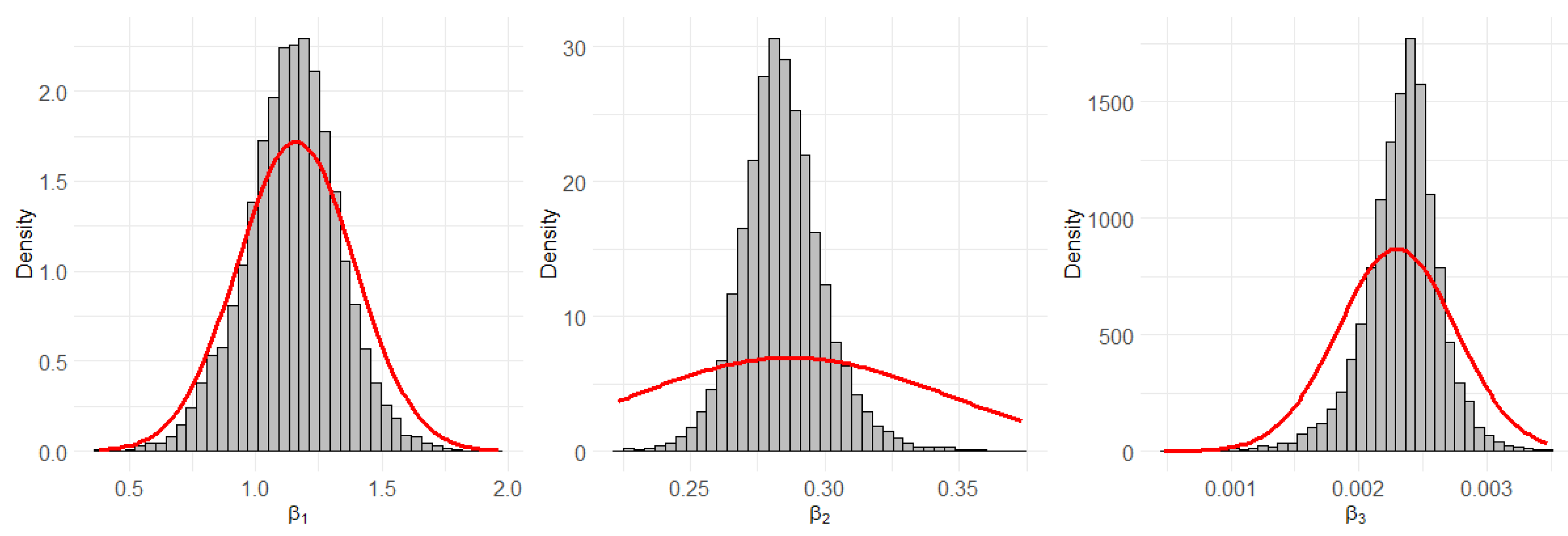The prior and posterior results for the $\mathit{\beta }$ parameters are shown in Figure 2. The prior distributions for the parameters ${\beta }_i$ are defined as normal distributions, with mean values obtained from the deterministic simulation model used to construct the surrogate.

Figure 2. Prior distributions (red curves) and posterior estimates (histograms) for $\beta$-parameters.

As shown, the prior distributions for the parameters ${\beta }_1$ and ${\beta }_3$ are more informative (less uncertain) compared to that of ${\beta }_2$. In contrast, the wider prior distribution for ${\beta }_2$ suggests higher uncertainty in its deterministic value, allowing for more flexibility in updating during the calibration process. The parameter ${\beta }_2$ is related to the deceleration rate in the context of stopping distance, which inherently involves variability and uncertainty. Using the training data, the parameters are then updated to obtain their posterior distributions, which reflect the refined estimates after incorporating the observed data.

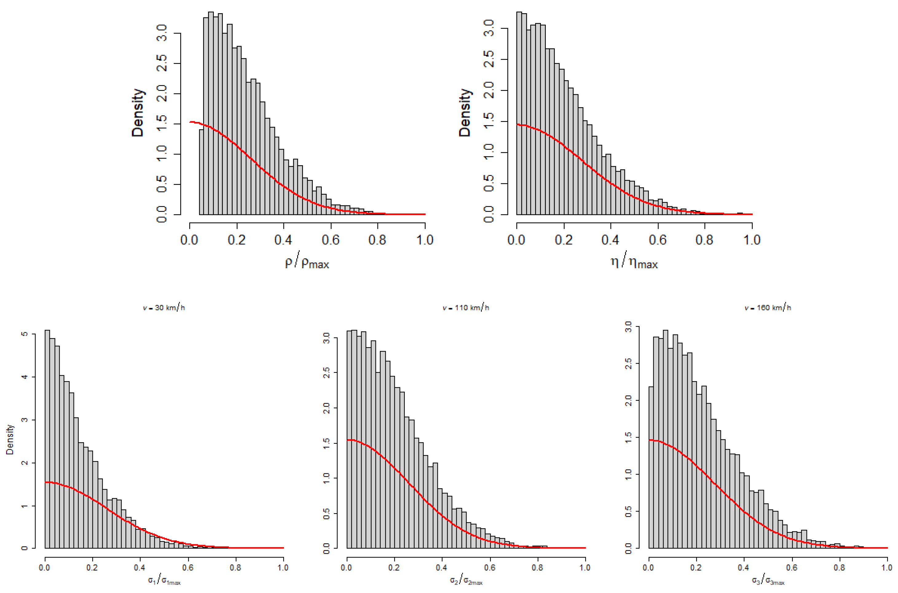
The prior and posterior densities of the kernel parameters ($\rho$, $\eta$, and $\sigma$) are shown in Figure 3, scaled with respect to their maximum values.

Figure 3. The prior (red curve) and the posterior (histogram) of kernel parameters (scaled): correlation length $\rho$ and deviation $\eta$ (upper row); $\sigma$ for calibration velocities 30, 110 and 160 km/h (lower row).

These distributions reflect the uncertainty in the parameter estimates after incorporating both prior knowledge and observed data. Initially, all kernel parameters are assumed to follow normal distributions, constrained to positive values. Notably, the correlation length $\rho$ is defined with a lower bound corresponding to the minimum difference between all training and testing velocities. Since the variance in the data is assumed to be heteroscedastic, individual $\sigma$ parameters are defined for each calibration velocity. The posterior density retains a similar range of values as the prior but exhibits a notable shift in its distributional form. While the prior follows a normal distribution, the posterior appears to transition towards an exponential-like shape. This suggests that the calibration data has significantly influenced the parameter’s distribution, introducing skewness and emphasizing smaller values within the feasible range.

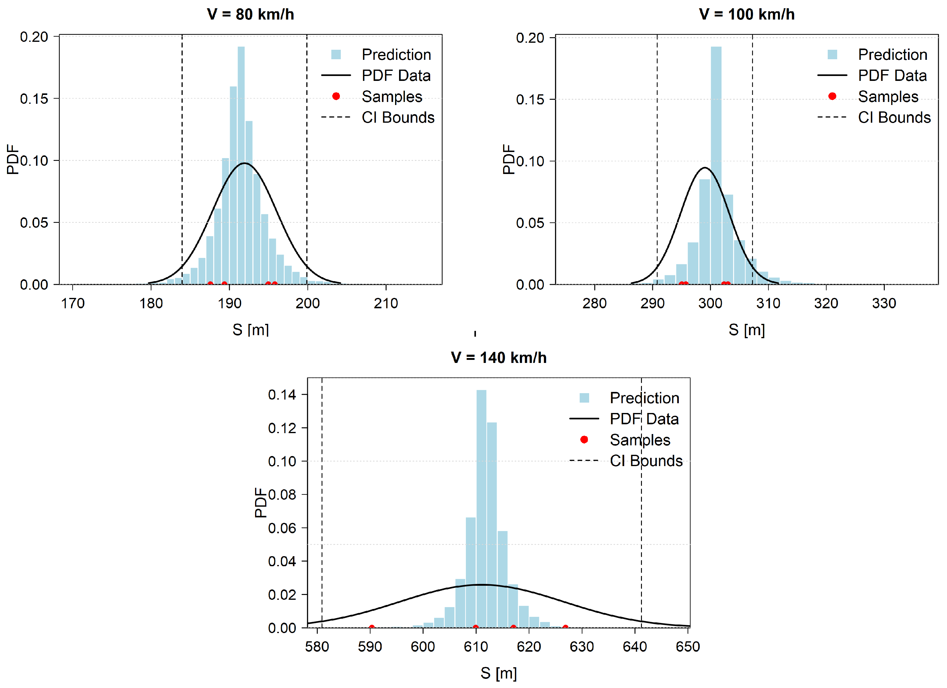
The results for the predicted stopping distances at the validated velocities are presented in Figure 4, along with the probability density functions (PDFs) of the corresponding measured samples.

Figure 4. Comparison of predicted stopping distances (posterior histogram) at 80, 100, and 140 km/h overlaid with the normal model of measurements (black curve).

The histograms represent the predicted stopping distances at the validation velocities of 80, 100, and 140 km/h. The solid black curves indicate the corresponding normal distributions of the measured stopping distances, modeled as $\mathcal{N}(\overline{s},\sigma )$, where $\sigma$ is defined as $3\%$ of the mean stopping distance $\overline{s}$ in accordance with the K1 criterion specified in EN 16834. $\overline{s}$ denotes the estimated mean of the stopping distances. The histograms are obtained from the model’s posterior predictive distribution, which accounts for both parameter uncertainty and observational noise in the predictions. The figure also includes the $95\%$ confidence intervals (CI) and the individual validation samples for reference. The overlap between the histogram and the black curve reflects the model’s predictive accuracy; a narrow, centered histogram indicates high confidence and good agreement with the measured data. Each validation group contains at least four tests, which is sufficient for K1/K2 evaluation but limits precise estimation of heteroskedastic noise. At 140 km/h the posterior predictive spread is narrower than the empirical scatter, indicating potential under-dispersion. Two remedies will be considered: (i) an explicit input-dependent noise model ${\sigma }^2\left(v\right)$ with monotonicity constraints; and (ii) kernels allowing scale variation across v. These are reflected in the narrower predictive distribution compared to the spread of the measured stopping distances. Such reduced uncertainty indicates that the model is more constrained and better informed at this velocity, due to consistent training data in this region.

Key numerical outcomes of the Bayesian predictions are summarized in Table 2. As observed, the predicted mean stopping distances closely match the sample means from the validation tests (values in parentheses), indicating high predictive accuracy. In addition, Table 2 reports the predicted standard deviations, coefficients of variation (CVs), and confidence intervals for the mean values. Notably, the Bayesian inference consistently yields CV values below $3\%$ across all validated velocities, satisfying the precision criteria stipulated in EN 16834.

Table 2. Summary of posterior predictions of stopping distance at validated velocities. Values in parentheses are sample means from the measured validation data. CI denotes the $95\%$ confidence interval for the posterior mean; cv denotes $({\sigma }_{\mathrm{pred}}/{\overline{s}}_{\mathrm{pred}})\times 100$ computed from the posterior predictive distribution.

v [km/h]	${\overline{\mathit{s}}}_{\mathbf{pred}}$ [m]	${\mathit{\sigma }}_{\mathbf{pred}}$ [m]	cv [%]	CI of Mean
80	191.5 (191.93)	3.19 (4.08)	1.67	[188.39, 194.62]
100	301.21 (299.03)	3.94 (4.22)	1.31	[297.37, 305.06]
140	611.88 (611.06)	3.91 (15.47)	0.64	[608.07, 615.69]

At 80 km/h and 100 km/h, the predicted stopping distance distributions show moderate spread and align well with the empirical data, indicating that the model effectively captures both the central tendency and variability of the observed behavior. At 140 km/h, however, the predictive distribution becomes notably narrower and more peaked, suggesting reduced posterior uncertainty. This contrasts with the wider spread of the test data at this speed, implying that the model underestimates real-world variability at higher velocities. The discrepancy could stem from limitations in capturing heteroskedasticity from training data in this range.

After training and testing (calibration and validation) on experimental data, the model demonstrates strong predictive capability for stopping distances at untested velocities. The results summarized in Table 3 illustrate the model’s performance for virtual test points at 90, 120, and 200 km/h, providing predicted mean stopping distances along with their associated uncertainties.

Table 3. Summary of predicted stopping distance statistics at virtual test velocities.

v [km/h]	${\overline{\mathit{s}}}_{\mathbf{pred}}$ [m]	sd [m]	cv [%]	CI of Mean
90	242.88	3.55	1.46	[237.65, 249.49]
120	440.65	3.65	0.83	[435.16, 447.6]
200	1341.82	11.93	0.89	[1315.16, 1364.61]

The predictions exhibit narrow credible intervals and low coefficients of variation, signifying consistent and reliable estimates across the tested velocity range. This ability to generalize effectively beyond the calibration data, while maintaining statistical rigor, positions the model as a valuable tool for uncertainty-aware virtual testing and the validation of railway brake performance.

5. Conclusions

We proposed a physics-informed Bayesian framework that fuses mechanistic brake thermodynamics and vehicle dynamics with Gaussian Process (GP) regression to deliver uncertainty-aware virtual testing. Embedding a calibrated physics surrogate as the GP mean and learning velocity-dependent covariance with heteroskedastic noise enables explicit decomposition of aleatoric and epistemic uncertainty and yields interpretable, standards-aligned predictions. Validation at 80, 100, and 140 km/h showed close agreement between posterior predictive means and test sample means, with predictive histograms aligning with empirical normal models, indicating robust calibration of both central tendency and dispersion. Coefficients of variation remained below 3% across validated speeds, satisfying EN 16834 K1, while predictive intervals were consistent with K2 bounds, supporting standards-compliant virtual verification. Posterior inference concentrated ${\beta }_1$ and ${\beta }_3$ (curvature and higher-order effects) and retained broader support for ${\beta }_2$ (deceleration sensitivity), matching physical intuition. Kernel posteriors favored shorter effective length-scales, reflecting sharper local correlation in velocity. Virtual tests at unobserved velocities produced narrow credible intervals and low CVs, demonstrating reliable interpolation within 30–160 km/h while preserving uncertainty quantification. Limitations include stationarity of the RBF kernel and reduced input dimensionality (velocity-only), which can underrepresent regime changes and cross-coupled thermomechanics; at 140 km/h, posterior spread was narrower than empirical variability, suggesting under-modeled heteroskedasticity or missing covariates. Future work will extend inputs (load, mode, temperatures, adhesion), adopt nonstationary/anisotropic or deep kernels, model input-dependent noise and multi-output responses (distance, deceleration, temperatures), introduce physics-informed kernels and state-space friction, and incorporate certification-oriented coverage guarantees and Bayesian optimal design. Overall, the framework delivers accurate, interpretable, and EN 16834-aligned virtual testing, with clear pathways to strengthen generalization and certification readiness in safety-critical dynamical systems.

While coefficients of variation remained <3% (K1), small sample sizes per speed and the stationary RBF kernel can under-represent real-world variability at high speeds. Future work will expand the dataset and adopt input-dependent noise and nonstationary kernels to improve uncertainty calibration.