Efficient Path Planning for Fiber Sorting Manipulators Based on Improved Bi-RRT* in Narrow Environments

Abstract

Automated foreign-fiber sorting in textile processing requires efficient robotic path planning, yet conventional sampling-based planners often struggle in narrow passages because of limited entrance accessibility and constrained tree expansion. To address this problem, this study proposes HA-Bi-RRT*, an improved Bi-RRT* planner incorporating a cooperative breakthrough mechanism, hybrid adaptive sampling, and hierarchical path refinement. When tree expansion is blocked, the cooperative mechanism guides the search along obstacle boundaries to facilitate passage-entrance localization. During passage traversal, the adaptive sampler enlarges the local sampling radius after consecutive failures to improve exploration around blocked regions. The method is evaluated in a two-dimensional benchmark, a three-dimensional narrow-passage environment, a ROS-based 5-DOF manipulator simulation, and a physical manipulator experiment. The observed results show favorable finite-budget trade-offs in planning success, runtime, and path cost relative to the selected baselines. The ROS simulation and physical experiments demonstrate the feasibility of converting the generated workspace paths into executable manipulator motions under the tested laboratory conditions.

1. Introduction

The textile industry is currently accelerating its transition towards Industry 4.0, focusing on boosting manufacturing intelligence and automation [1]. Within this context, automated foreign-fiber sorting has emerged as a critical step to ensure product quality. The ultimate goal of this momentum is to utilize robotic arms for the precise grasping of foreign fibers in complex environments [2]. To achieve such precise grasping, deep learning-based foreign-fiber detection systems have matured to achieve high-precision identification [3,4]. However, relying exclusively on visual detection is insufficient; the automated sorting process inherently requires path planning to play a crucial connecting role. By translating visual localization results into specific motion commands, the path planning algorithm ensures successful obstacle avoidance and precise target reaching for the robotic arm, thereby directly determining the efficiency and safety of the foreign-fiber sorting system [5].

Path planning spans several established families of methods. A* uses heuristic estimates to search graphs for minimum-cost paths [6], while D* updates plans efficiently when the environment is only partially known or changes during navigation [7]. The artificial potential field (APF) method guides motion through attraction to the goal and repulsion from obstacles [8]. Later work improved APF to address goal unreachability and local minima in mobile-robot planning [9], and combined improved APF with RRT to exploit the complementary strengths of potential-field guidance and tree-based exploration [10]. These studies establish useful search and guidance principles; for the confined sorting workspace considered here, sampling-based planning offers a flexible basis for investigating narrow-passage traversal.

Among these approaches, sampling-based methods are widely used for robotic manipulation. Algorithms represented by PRM [11] and RRT [12] are attractive because they avoid full-space discretization and can handle complex planning domains. Under standard assumptions, these methods are probabilistically complete, meaning that the probability of finding a feasible solution approaches one as the number of samples increases when such a solution exists. However, in narrow-passage scenarios for fiber sorting, uniform sampling faces two related challenges: locating a small passage entrance and sustaining valid tree growth within the constrained region. These challenges lead to a scarcity of useful samples and may cause search stagnation [13,14,15,16].

To address the narrow passage problem, researchers have explored several distinct strategies, each embodying a fundamental trade-off between computational speed, environmental adaptability, and prior knowledge requirements. Within the sampling optimization paradigm, the prevailing approach has been to progressively constrain the search space. Gammell et al. [17] pioneered this direction with Informed-RRT*, which concentrates samples within an ellipsoidal domain defined by the current best path length. Adaptive successors such as AI-RRT [18] pushed this further by continuously shrinking the heuristic region, while density-sensitive frameworks such as MINER-RRT* [19] modulated local sampling density according to obstacle proximity. ACO-based variants [20] introduced pheromone-guided search to iteratively refine path quality. However, for sampling distribution optimization methods, their shared reliance on the statistical regularity of uniform sampling becomes a critical liability in extremely narrow passages, often resulting in slow convergence or outright initial sampling failure.

To reduce the blindness of random sampling, geometric guidance methods offer a more deterministic alternative. Rather than relying on samples to encounter narrow openings, skeleton-guided methods [21] precompute guidance corridors by extracting topological structures from the workspace. Supplementary techniques such as B-spline path smoothing [22] and boundary-reactive steering corrections [23,24] further improve behavior in confined spaces. However, global map preprocessing introduces additional computational cost and may be unsuitable for time-sensitive online planning.

Beyond conventional sampling optimization and geometric guidance, researchers have investigated learned and hybrid strategies. GAN-based heuristics learn to bias the sampling distribution [25]. RJ-RRT dynamically reduces the sampling space and explores identified narrow passages with subtrees [26]. Bi-RRT* trajectory optimization for serial manipulators [27], planners that balance exploration and exploitation [28], and APF-RRT hybrids [29] offer other forms of search or path guidance. MPNet uses a learned representation of the environment to propose motion paths [30]. Learned approaches depend on representative training data, while heuristic variants have distinct design and tuning requirements; the extent to which either class can reliably locate and traverse very narrow openings remains task-dependent.

Existing narrow-passage planners commonly improve either passage discovery, local traversal, or post-processing, but these stages are often treated separately. GDRRT* accelerates target-directed exploration by adapting its sampling range according to goal distance [31], but it does not explicitly reuse repeated collision failures as local passage cues. HA-Bi-RRT* instead couples boundary expansion with feedback-driven sampling and collision-aware path refinement. Unlike skeleton-guided methods, it does not require global skeleton preprocessing; unlike fixed bridge or tunnel samplers, its local sampling behavior is updated from recent tree-growth feedback.

Accordingly, this paper proposes HA-Bi-RRT*, a Bi-RRT*-based planner designed to improve finite-budget planning efficiency, success rate, and path quality in constrained environments. The main contributions are summarized as follows:

To solve the problem of geometric guidance strategies in irregular gaps, a cooperative breakthrough mechanism is designed. When the search is blocked, this mechanism guides the random tree to extend along the obstacle contours, achieving “wall-following” traversal without the need for precise geometric modeling.

To improve dynamic adaptability in confined spaces, a hybrid adaptive sampling strategy is developed. This strategy integrates centroid tracking with a dynamic sampling domain based on historical success rates, enabling the algorithm to switch efficiently between global exploration and local narrow passage breakthrough.

A hierarchical geometric path-refinement method combines global dynamic-programming shortcutting with local collision-aware shortcutting to remove redundant waypoints. This stage improves path length and compactness; it does not optimize velocity, acceleration, jerk, or execution time.

2. Wool–Cashmere Foreign-Fiber Sorting Task and Motion-Planning Formulation

2.1. Vision-Guided Sorting Workflow and Planning Interface

The proposed HA-Bi-RRT* planner is embedded in a vision-guided robotic workflow for wool–cashmere foreign-fiber sorting, as illustrated in Figure 1. First, the material scene is acquired by the vision system, and the foreign-fiber target is detected and localized. The detected position is then transformed into the manipulator coordinate system. Based on the current manipulator state and workspace obstacle constraints, HA-Bi-RRT* generates collision-free geometric paths for the approach, grasp, transfer, and removal stages.

As shown in Figure 1, the complete sorting workflow consists of a perception layer, a workspace motion-planning layer, and a manipulator-execution stage. Let ${\mathrm{q}}_{\mathrm{c}\mathrm{u}\mathrm{r}}$ denote the measured joint configuration of the manipulator. The corresponding end-effector position is obtained through forward kinematics and used as the workspace start point ${\mathrm{x}}_{\mathrm{s}\mathrm{t}\mathrm{a}\mathrm{r}\mathrm{t}}$. The detected foreign-fiber position, after camera calibration and coordinate transformation, defines the workspace goal point ${\mathrm{x}}_{\mathrm{g}\mathrm{o}\mathrm{a}\mathrm{l}}$. Let M denote the workspace obstacle map. HA-Bi-RRT* receives ${\mathrm{x}}_{\mathrm{s}\mathrm{t}\mathrm{a}\mathrm{r}\mathrm{t}}$, ${\mathrm{x}}_{\mathrm{g}\mathrm{o}\mathrm{a}\mathrm{l}}$, and M as inputs and generates a collision-free geometric path ${\mathrm{\pi }}^{*}$ in the Cartesian workspace. During robot execution, the workspace waypoints are mapped into the reachable region and converted into joint targets through inverse kinematics.

The process used to generate the motion-planning target from the wool–cashmere material image is illustrated in Figure 2. The purpose of this process is to establish a concise interface between foreign-fiber perception and manipulator motion planning, rather than to develop a separate visual-detection method.

As shown in Figure 2, the foreign-fiber target is first identified in the acquired wool–cashmere image. Because foreign fibers generally have irregular or elongated geometries, the target center and principal orientation are extracted to determine the grasp point and end-effector approach direction. The image-space grasp point is then mapped into the manipulator base coordinate system through camera calibration and coordinate transformation. The resulting Cartesian target position defines ${\mathrm{x}}_{\mathrm{g}\mathrm{o}\mathrm{a}\mathrm{l}}$ for workspace path planning, while the desired end-effector orientation is specified separately as an execution constraint. After a collision-free workspace path has been obtained, its waypoints are converted into joint targets through inverse kinematics.

2.2. Manipulator Kinematic Model

After the foreign-fiber target pose is obtained, a manipulator kinematic model is required to convert the planned Cartesian waypoints into executable joint targets. The D–H coordinate-frame assignment of the 5-DOF Dobot manipulator is shown in Figure 3. The kinematic model of the 5-DOF Dofbot manipulator therefore provides the geometric basis for forward-kinematic initialization, inverse-kinematic conversion, and trajectory execution. It does not define the search space of HA-Bi-RRT*, which remains a two-dimensional or three-dimensional Cartesian workspace. Because HA-Bi-RRT* performs geometric planning in the Cartesian workspace, the planner itself is not explicitly parameterized by the number of manipulator joints. In principle, the same workspace planning interface can be coupled with manipulators of different DOFs, provided that an appropriate inverse-kinematics solver, joint-limit model, and collision-checking model are available in the execution layer. However, this study validates this interface only on the 5-DOF Dofbot platform; therefore, performance and executability on higher-DOF manipulators are not experimentally established and should be evaluated in future work.

Figure 3. D-H coordinate-frame assignment of the 5-DOF Dofbot manipulator.

Figure 3. D-H coordinate-frame assignment of the 5-DOF Dofbot manipulator.

The spatial relationship between two adjacent coordinate frames is described by the four standard D–H parameters: link length, link twist, link offset, and joint angle. According to the physical structure of the manipulator, the parameters are listed in

Table 1. Standard D–H parameters of the 5-DOF manipulator.

i	${\mathbf{d}}_{\mathbf{i}}$ (m)	${\mathbf{a}}_{\mathbf{i}}$ (m)	${\mathsf{\alpha }}_{\mathbf{i}}$ (rad)	${\mathsf{\theta }}_{\mathbf{i}}$ (rad)
1	0.066	0	0	${\mathrm{\theta }}_1$
2	0.04145	0	$\mathrm{\pi }/2$	${\mathrm{\theta }}_2$
3	0	−0.08285	0	${\mathrm{\theta }}_3$
4	0	−0.08285	0	${\mathrm{\theta }}_4$
5	0	−0.07385	$-\mathrm{\pi }/2$	${\mathrm{\theta }}_5$

.

The homogeneous transformation matrix ${}_{\mathrm{i}}{}^{\mathrm{i}-1}\mathrm{T}$ relating frame $\left\{\mathrm{i}\right\}$ to frame $\{\mathrm{i}-1\}$ is formulated as:

$${}_{\mathrm{i}}{}^{\mathrm{i}-1}\mathrm{T}=\left[\begin{array}{cccc}\cos {\mathrm{\theta }}_{\mathrm{i}}& -\sin {\mathrm{\theta }}_{\mathrm{i}}\cos {\mathrm{\alpha }}_{\mathrm{i}}& \sin {\mathrm{\theta }}_{\mathrm{i}}\sin {\mathrm{\alpha }}_{\mathrm{i}}& {\mathrm{a}}_{\mathrm{i}}\cos {\mathrm{\theta }}_{\mathrm{i}}\\ \sin {\mathrm{\theta }}_{\mathrm{i}}& \cos {\mathrm{\theta }}_{\mathrm{i}}\cos {\mathrm{\alpha }}_{\mathrm{i}}& -\cos {\mathrm{\theta }}_{\mathrm{i}}\sin {\mathrm{\alpha }}_{\mathrm{i}}& {\mathrm{a}}_{\mathrm{i}}\sin {\mathrm{\theta }}_{\mathrm{i}}\\ 0& \sin {\mathrm{\alpha }}_{\mathrm{i}}& \cos {\mathrm{\alpha }}_{\mathrm{i}}& {\mathrm{d}}_{\mathrm{i}}\\ 0& 0& 0& 1\end{array}\right]$$

(1)

By multiplying the transformation matrices of all joints, the forward kinematics of the manipulator can be obtained as:

$${}_5{}^0\mathrm{T}(\mathrm{q}){ = }_1^0\mathrm{T}({\mathrm{\theta }}_1{)}_2^1\mathrm{T}({\mathrm{\theta }}_2{)}_3^2\mathrm{T}({\mathrm{\theta }}_3{)}_4^3\mathrm{T}({\mathrm{\theta }}_4{)}_5^4\mathrm{T}({\mathrm{\theta }}_5)$$

(2)

where $\mathrm{q}=[{\mathrm{\theta }}_1,{\mathrm{\theta }}_2,{\mathrm{\theta }}_3,{\mathrm{\theta }}_4,{\mathrm{\theta }}_5{]}^{\mathrm{T}}$ denotes the joint configuration vector. The forward-kinematics model maps the measured joint state to the Cartesian end-effector pose, whereas inverse kinematics converts the planned workspace waypoints into joint targets for execution. The vector $\mathrm{q}$ is used by the kinematic conversion and execution layer and is not directly sampled by HA-Bi-RRT*.

2.3. Workspace and Collision Modeling for Wool–Cashmere Sorting

To construct the map required by HA-Bi-RRT*, the physical wool–cashmere foreign-fiber sorting scene is abstracted into a geometric workspace model. As illustrated in Figure 4, the detected foreign-fiber position defines the task target, while the sorting-tray boundaries, supporting frame, fixed workspace structures, and receiving container are represented as obstacle constraints. The current end-effector position provides the workspace start point, and the target grasp position provides the workspace goal point.

In Figure 4a, the foreign-fiber target is identified in the wool–cashmere material scene. Figure 4b shows the corresponding manipulator workcell, including the material tray, manipulator, supporting structures, and receiving container. These components are converted into the simplified obstacle representation in Figure 4c. The green and red nodes denote the workspace start and goal points, respectively, while the gray regions represent non-traversable obstacles. The narrow free region between the obstacles is the constrained passage explored by the planner. The illustrated curve is a schematic feasible path rather than an experimental result.

The HA-Bi-RRT* search is performed in a geometric Cartesian workspace. Let $\mathrm{X}\subset {\mathrm{R}}^{\mathrm{d}}$ denote the planning domain, where $\mathrm{d}=2$ for Scenario 1 and $\mathrm{d}=3$ for Scenario 2 and the ROS planning environment. Let ${\mathrm{O}}_{\mathcal{l}}$ denote the region occupied by the $\mathcal{l}$-th obstacle, and let ${\mathrm{n}}_{\mathrm{o}}$ be the number of obstacles. The total obstacle region is defined as

$$\mathrm{O}={\cup }_{\mathcal{l}=1}^{{\mathrm{n}}_{\mathrm{o}}}{\mathrm{O}}_{\mathcal{l}}$$

(3)

To account for the required collision clearance, the geometric obstacles are expanded by a safety region $\mathrm{B}({\mathrm{r}}_{\mathrm{s}})$, where ${\mathrm{r}}_{\mathrm{s}}$ denotes the prescribed safety margin. The resulting obstacle region used for collision checking is

$${\mathrm{X}}_{\mathrm{o}\mathrm{b}\mathrm{s}}=\mathrm{O}\oplus \mathrm{B}({\mathrm{r}}_{\mathrm{s}})$$

(4)

where $\oplus$ denotes the Minkowski sum. The collision-free planning region is therefore

$${\mathrm{X}}_{\mathrm{f}\mathrm{r}\mathrm{e}\mathrm{e}}=\mathrm{X}\setminus {\mathrm{X}}_{\mathrm{o}\mathrm{b}\mathrm{s}}$$

(5)

A workspace point is feasible if it lies in ${\mathrm{X}}_{\mathrm{f}\mathrm{r}\mathrm{e}\mathrm{e}}$, and an edge between two tree nodes is feasible if the corresponding line segment remains entirely within ${\mathrm{X}}_{\mathrm{f}\mathrm{r}\mathrm{e}\mathrm{e}}$. Narrow passages occupy only a small portion of this collision-free workspace, which reduces the probability of obtaining useful random samples and increases the frequency of blocked tree extensions.

2.4. Workspace Path-Planning Problem Statement

During each foreign-fiber removal cycle, the current end-effector position obtained through forward kinematics defines ${\mathrm{x}}_{\mathrm{s}\mathrm{t}\mathrm{a}\mathrm{r}\mathrm{t}}$, while the detected and calibrated foreign-fiber position defines ${\mathrm{x}}_{\mathrm{g}\mathrm{o}\mathrm{a}\mathrm{l}}$. Depending on the execution stage, ${\mathrm{x}}_{\mathrm{g}\mathrm{o}\mathrm{a}\mathrm{l}}$ may represent a pre-grasp point, a grasp point, or a transfer point above the receiving container.

Given ${\mathrm{x}}_{\mathrm{s}\mathrm{t}\mathrm{a}\mathrm{r}\mathrm{t}}\in {\mathrm{X}}_{\mathrm{f}\mathrm{r}\mathrm{e}\mathrm{e}}$ and ${\mathrm{x}}_{\mathrm{g}\mathrm{o}\mathrm{a}\mathrm{l}}\in {\mathrm{X}}_{\mathrm{f}\mathrm{r}\mathrm{e}\mathrm{e}}$, the objective is to determine a continuous collision-free workspace path connecting the two points. For a discrete path $\mathrm{\pi }={\mathrm{x}}_1,{\mathrm{x}}_2,\dots ,{\mathrm{x}}_{\mathrm{m}}$, where ${\mathrm{x}}_1={\mathrm{x}}_{\mathrm{s}\mathrm{t}\mathrm{a}\mathrm{r}\mathrm{t}}$ and ${\mathrm{x}}_{\mathrm{m}}={\mathrm{x}}_{\mathrm{g}\mathrm{o}\mathrm{a}\mathrm{l}}$, the path cost is defined as

$$\mathrm{J}(\mathrm{\pi })={\sum }_{\mathrm{j}=1}^{\mathrm{m}-1}{\left|{\mathrm{x}}_{\mathrm{j}+1}-{\mathrm{x}}_{\mathrm{j}}\right|}_2.$$

(6)

A lower path cost indicates a shorter workspace path with fewer redundant detours. The planning objective is therefore to find a feasible path with low workspace path cost while satisfying collision-avoidance and clearance constraints. After planning, the workspace waypoints are mapped and converted into joint targets for manipulator execution.

3. HA-Bi-RRT* Algorithm

3.1. Framework of HA-Bi-RRT* Algorithm

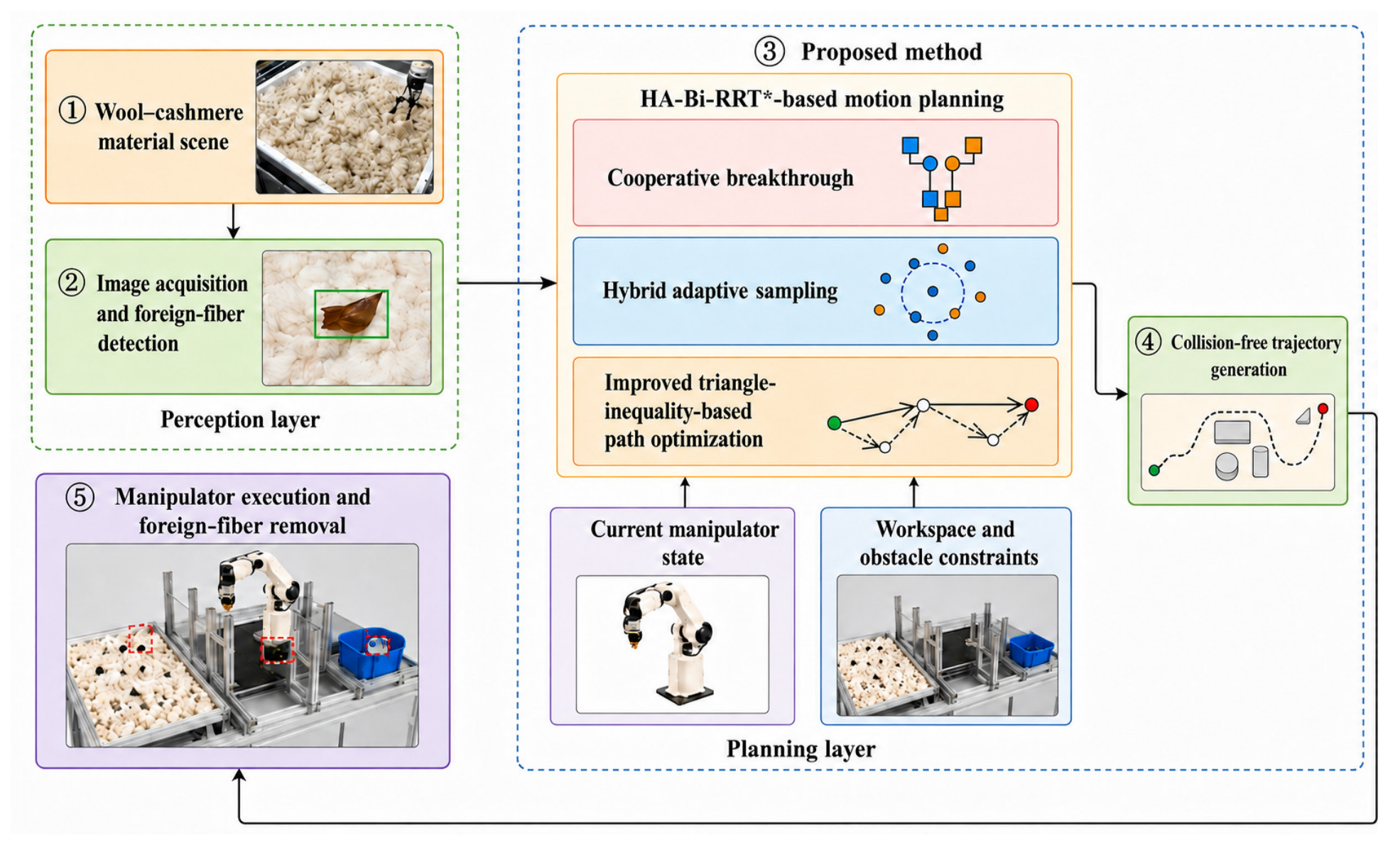
To address narrow-passage planning in fiber-sorting manipulation, this paper proposes HA-Bi-RRT*, a failure-informed adaptive planner based on Bi-RRT*. Instead of discarding failed extensions, HA-Bi-RRT* reuses blocked boundary nodes to guide later exploration.

Because its adaptive sampling and deterministic boundary-expansion policies differ from standard RRT*, this study does not claim a formal asymptotic-optimality guarantee for HA-Bi-RRT*. The evaluation therefore focuses on finite-budget success rate, runtime, search effort, and workspace path cost.

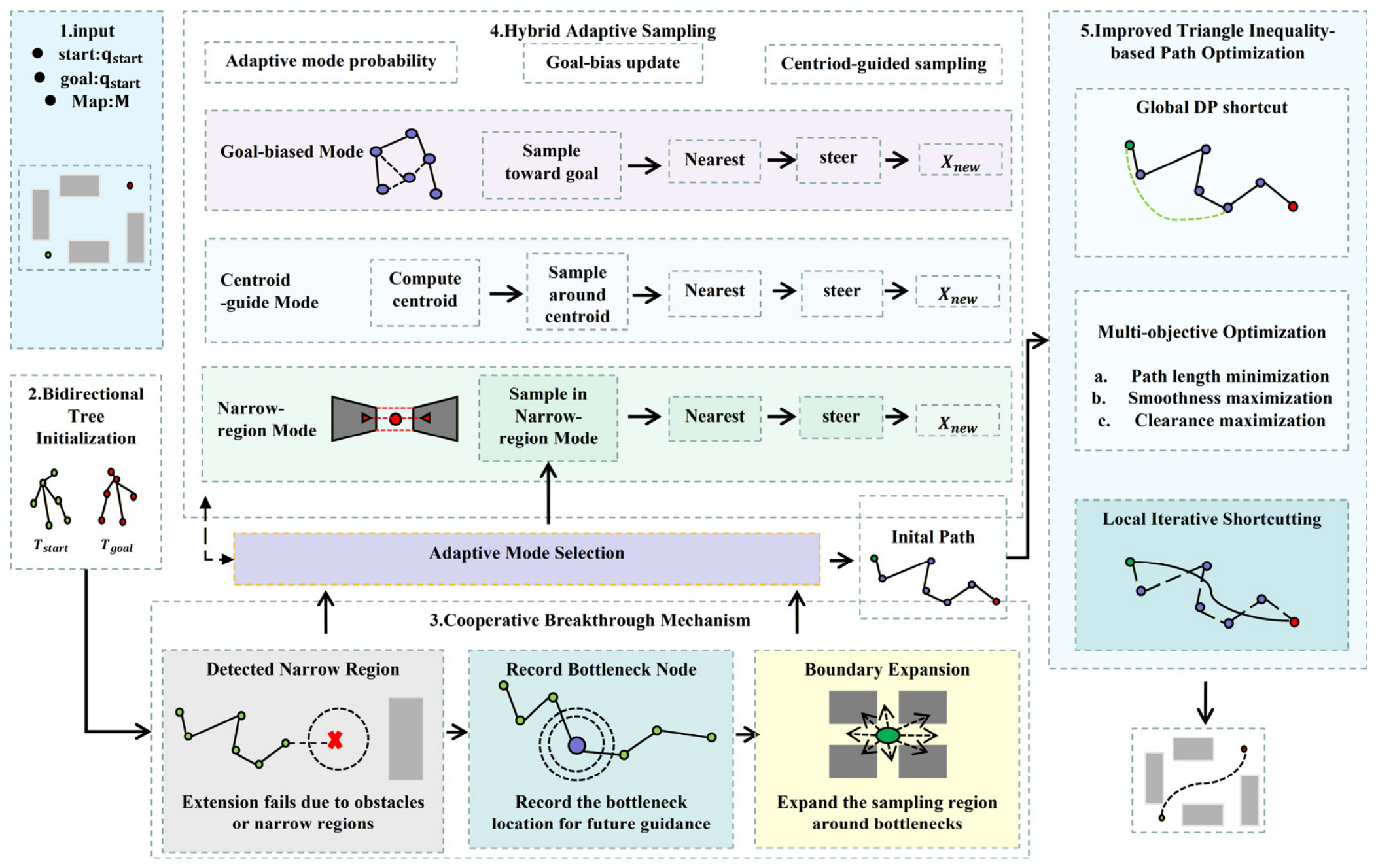
As shown in Figure 5, HA-Bi-RRT* contains three modules: cooperative breakthrough, hybrid adaptive sampling, and hierarchical path refinement. The cooperative breakthrough module reuses blocked boundary nodes for obstacle-boundary expansion. The hybrid sampler switches among goal-biased, centroid-guided, and narrow-region sampling according to tree-growth feedback. The refinement module removes redundant waypoints and improves path compactness.

The overall procedure of HA-Bi-RRT* is summarized in Algorithm 1.

Algorithm 1. HA-Bi-RRT* Main Framework
Input: Start point $x_{start},$ Goal point $x_{goal},$ map M, maximum Iteration $N_{max},$ connection threshold ε Output: refined path ${\pi }^{*}$
1	Initialize two trees $T_{start}\leftarrow x_{start}, T_{goal}\leftarrow x_{goal}$
2	Initialize narrow-region memory $N_{reg}$← ∅
3	Initialize best path π* ← ∅ and best cost c* ← ∞.
4	for k = 1 to N_max do
5	if k is odd then
6	$T_{curr}$ ← $T_{start},$ $T_{other}$ ← $T_{goal},$ $x_{target}$ ← $x_{goal}.$
7	else
8	$T_{curr}$ ← $T_{goal},$ $T_{other}$ ← $T_{start},$ $x_{target}$ ←$x_{start}.$
9	end if
10	$x_{rand}$ ← HybridAdaptiveSampling($T_{curr},$ $x_{target},$ $N_{reg}$).
11	$x_{near}$ ← Nearest$(T_{curr},$ $x_{rand}$).
12	$x_{new}$ ← Steer$(x_{near},$ $x_{rand}$).
13	if CollisionFree$(x_{near},$ $x_{new},$ M) then
14	InsertNode$(T_{curr},$ $x_{new},$ $x_{near}$).
15	Rewire$(T_{curr},$ $x_{new}$).
16	else
17	RecordNarrowRegion$(N_{reg},$ $x_{near}$).
18	$x_{bound}$ ← BoundaryExpansion$(x_{near},$ M).
19	if x_bound ≠ NULL then
20	InsertNode$(T_{curr},$ $x_{bound},$ $x_{near}$).
21	$x_{new}$ ← $x_{bound}.$
22	else
23	continue.
24	end if
25	end if
26	$x_{conn}$ ← Nearest$(T_{other},$ $x_{new}$).
27	if$\Vert x_{new}$ $- x_{conn}$ $\Vert < \epsilon and CollisionFree(x_{new},$ $x_{conn},$ M) then
28	${\pi }_{curr}$ ← ConstructPath$(T_{curr},$ $T_{other},$ $x_{new},$ ${ x}_{conn}$).
29	if Cost$({\pi }_{curr}$) < c* then
30	π* ← ${\pi }_{curr},$ c* ← Cost$({\pi }_{curr}$).
31	end if
32	end if
33	if π* ≠ ∅ and QualityStop(c*/c_min, k/N_max) then break.
34	end for
35	if π* ≠ ∅ then π* ← HierarchicalPathRefinement(π*).
36	return π*.

Algorithm 1 initializes two trees from the start and goal configurations. In each iteration, the hybrid sampler generates a candidate sample, and the selected tree extends toward it through nearest-neighbor search, steering, and collision checking. If the extension is blocked, the cooperative breakthrough mechanism records the blocked node and attempts boundary expansion. If the two trees connect, the resulting feasible path replaces the incumbent if its cost is lower. The search continues until a shared hard limit or the shared quality-based early-stop rule is reached; the retained path is then passed to hierarchical path refinement.

In Algorithm 1, $N_{max}$ denotes the shared maximum-iteration limit. The connection threshold ε in line 27 is the maximum Euclidean separation allowed between the nearest nodes of the two trees before the straight connecting segment is checked for collision; a connection is accepted only when both the distance and collision-free conditions are satisfied. Here, $T_{curr}$ and $T_{other}$ denote the currently expanded tree and the opposite tree, respectively; $x_{target}$ is the active target of the current expansion; $x_{rand}$, $x_{near}$ and $x_{new}$ denote the sampled point, nearest tree node, and newly generated node, respectively; $x_{bound}$ is the node generated by boundary expansion, and $x_{conn}$ is the nearest node in the opposite tree used for tree connection. The loop shown in Algorithm 1 is also subject to the generated-node and timeout limits in

Table 2. Common experimental settings for all planners.

Parameter	Scenario 1	Scenario 2	ROS Simulation
Workspace size	50 cm × 50 cm	50 cm × 50 cm × 30 cm	50 cm × 50 cm × 30 cm workspace
Maximum iterations	10,000	10,000	10,000
Maximum nodes	5000	5000	5000
Timeout threshold	5 s	10 s	10 s
Number of independent trials	100	100	—

Note: The 100-trial protocol applies to the two geometric benchmark scenarios only; the ROS simulation is a representative execution-feasibility demonstration rather than a repeated-trial statistical benchmark.

; finding a feasible path does not itself end the search.

For the geometric comparisons, every planner used the same quality-based early-stop rule in addition to the hard limits in Table 2. Let $\rho =c^{*}/c_{min}$, where c* is the cost of the current best feasible path and c_min is the straight-line start–goal distance. Once more than 20%, 30%, or 40% of the maximum iteration count had elapsed, respectively, the search could stop if $\rho$ < 1.10, $\rho$ < 1.15, or $\rho$ < 1.20. The first feasible path therefore establishes an incumbent but is not itself a stopping event. After the search terminates, HA-Bi-RRT* applies its hierarchical path-refinement stage.

3.2. Cooperative Breakthrough Mechanism

Traditional RRT-based planners often stagnate near narrow passages because random samples rarely fall inside small feasible gaps. When an extension is blocked, the failed attempt is usually discarded. In contrast, HA-Bi-RRT* treats such failures as useful boundary information.

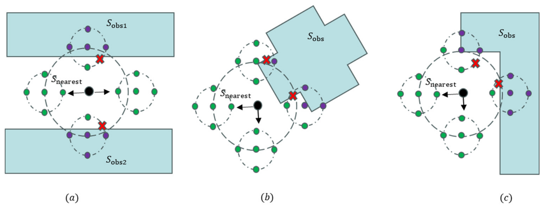
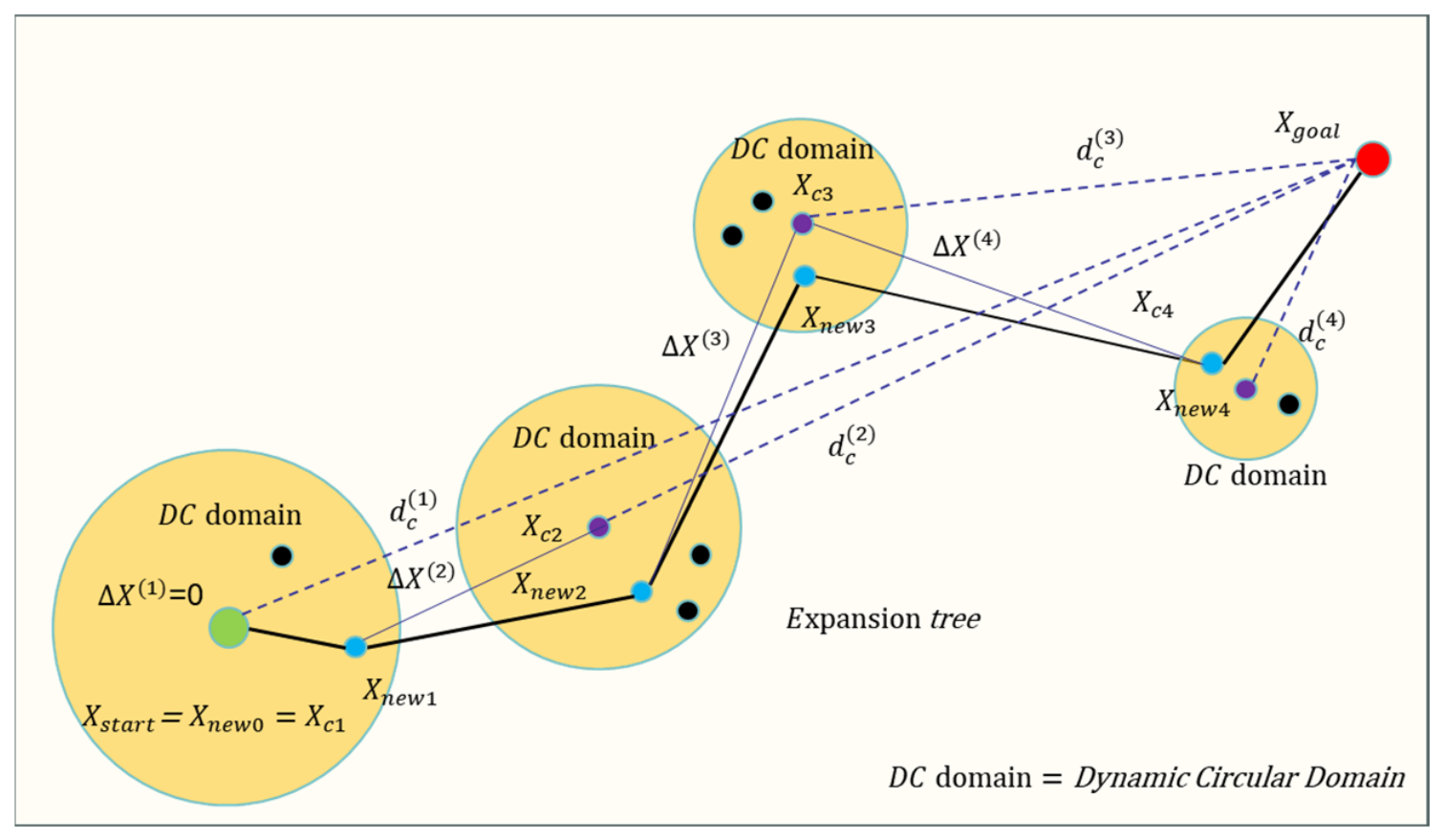
When the extension from ${\mathrm{x}}_{\mathrm{n}\mathrm{e}\mathrm{a}\mathrm{r}}$ to ${\mathrm{x}}_{\mathrm{r}\mathrm{a}\mathrm{n}\mathrm{d}}$ is blocked, the planner records ${\mathrm{x}}_{\mathrm{n}\mathrm{e}\mathrm{a}\mathrm{r}}$ as a bottleneck candidate in the narrow-region memory. It then probes several directions around this node and attempts a short boundary expansion. If a collision-free direction is found, the tree continues to grow along the obstacle boundary instead of stopping at the blocked point. This mechanism turns a failed extension into a local search cue and helps the tree approach narrow-passage entrances more steadily.

As shown in Figure 6, the boundary node cannot directly extend toward the random sample because of obstacle blockage. The proposed boundary expansion probes multiple local directions and selects a feasible direction if one exists. Assuming that the success probability of one probing direction is p_single, the probability of obtaining at least one feasible extension among n directions is

$${\mathrm{P}}_{\mathrm{s}\mathrm{u}\mathrm{c}\mathrm{c}\mathrm{e}\mathrm{s}\mathrm{s}}=1-(1-{\mathrm{p}}_{\mathrm{s}\mathrm{i}\mathrm{n}\mathrm{g}\mathrm{l}\mathrm{e}}{)}^{\mathrm{n}}$$

(7)

This probability increases with the number of probing directions, which explains why local boundary probing can improve passage traversal.

3.3. Hybrid Adaptive Sampling

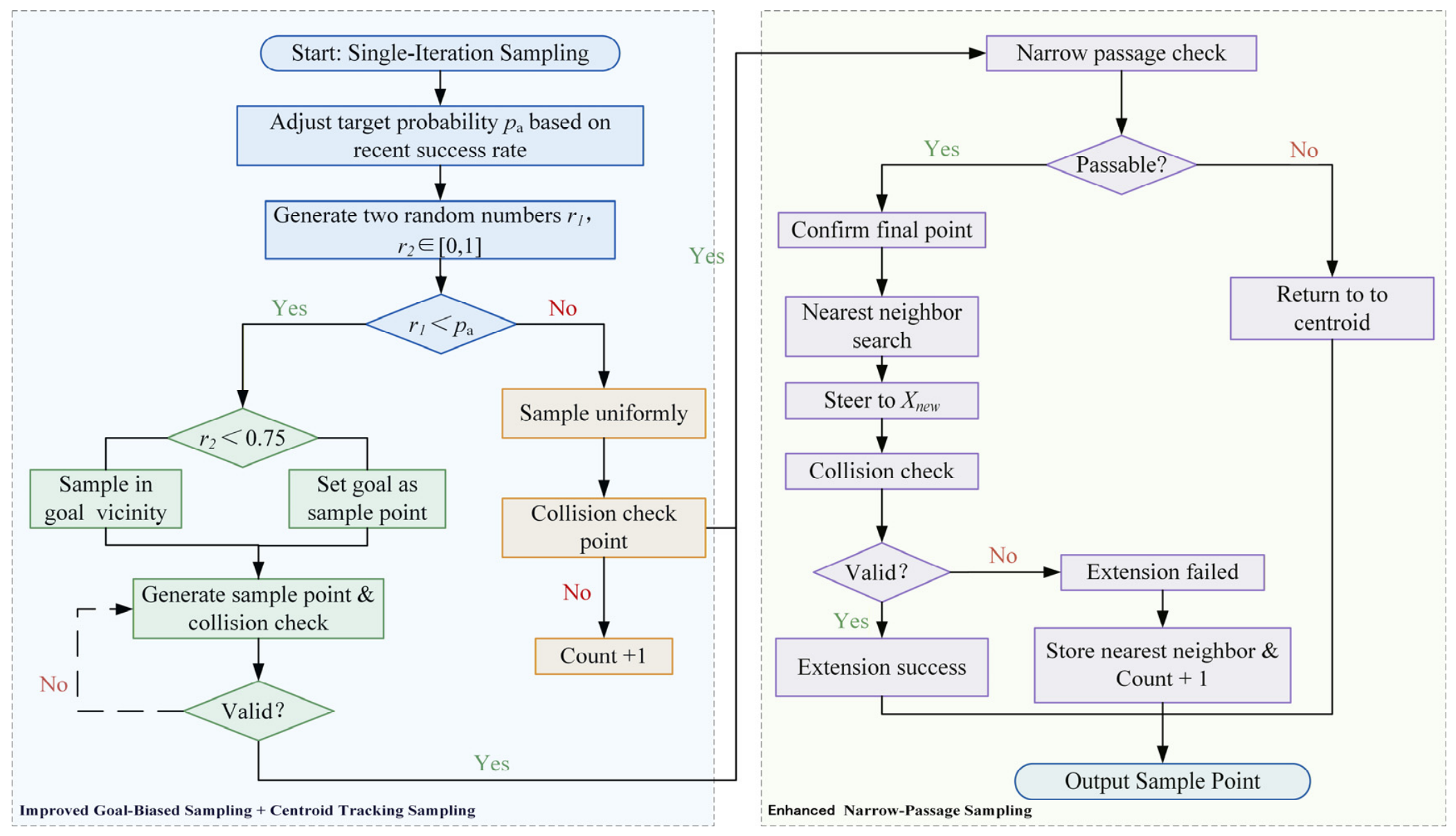
The hybrid adaptive sampler balances global search and local passage exploration. It contains three sampling modes: goal-biased sampling, centroid-guided sampling, and narrow-region sampling. The planner selects the sampling mode according to recent tree-growth feedback and the recorded narrow-region memory.

As shown in Figure 7, goal-biased sampling accelerates convergence when the search is smooth. Centroid-guided sampling keeps the sampling region close to the current tree-growth direction. Narrow-region sampling is activated when repeated extension failures indicate a possible passage entrance. This switching strategy helps the planner avoid blind uniform sampling while preserving global exploration.

3.3.1. Adaptive Goal-Biased Sampling

A fixed goal-bias probability is not suitable for narrow-passage planning. In open regions, a larger goal bias helps the tree move quickly toward the target. Near obstacles, however, excessive goal bias may repeatedly pull the tree toward blocked directions. Therefore, HA-Bi-RRT* adjusts the goal-bias probability according to the recent extension success rate.

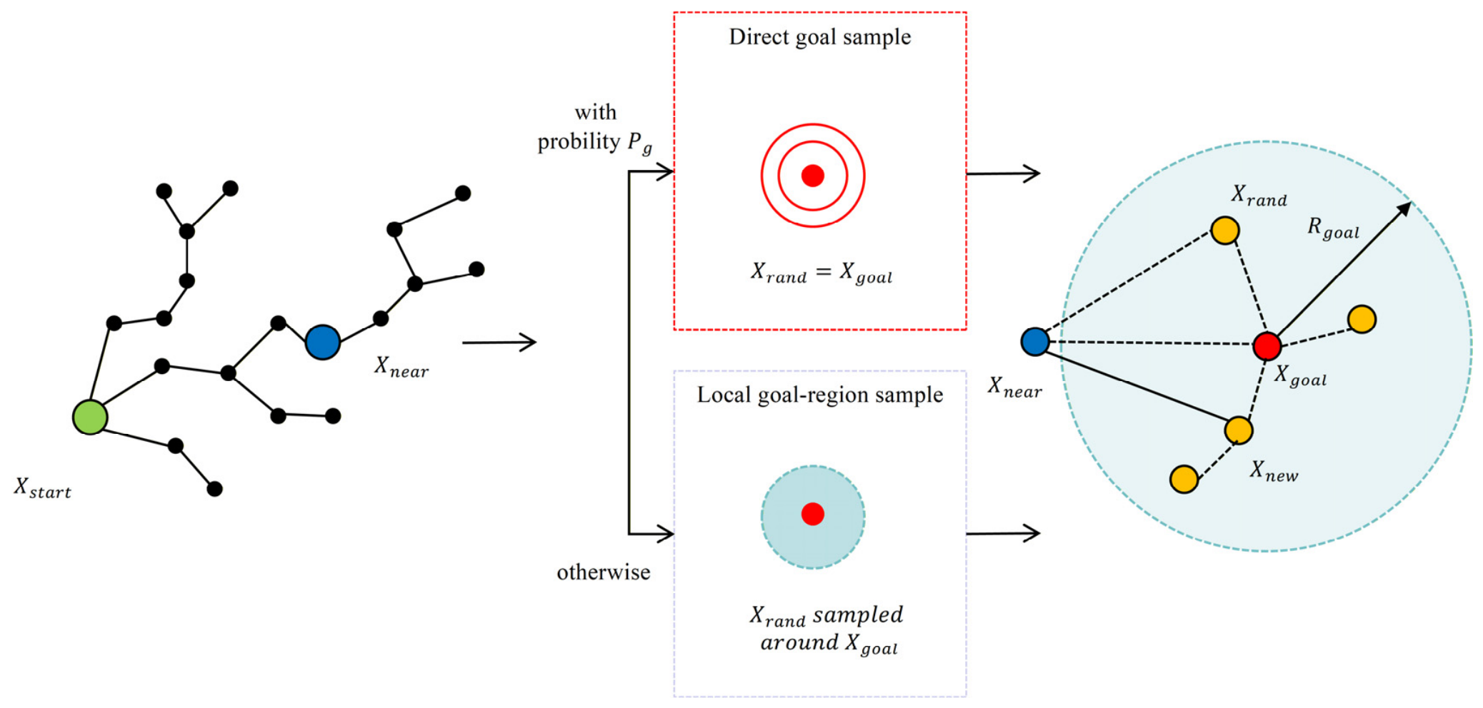
As shown in Figure 8, the planner uses two target-oriented sampling modes. With probability $p_g$, the active target itself is selected; otherwise, a sample is generated in a local region around the active target. This design preserves goal attraction while maintaining local randomness around the target. The sampling model is defined as

$${\mathrm{x}}_{\mathrm{r}\mathrm{a}\mathrm{n}\mathrm{d}}=\left\{\begin{array}{ll}{\mathrm{x}}_{\mathrm{t}\mathrm{a}\mathrm{r}\mathrm{g}\mathrm{e}\mathrm{t}},& \mathrm{u}<{\mathrm{p}}_{\mathrm{g}}\\ {\mathrm{x}}_{\mathrm{t}\mathrm{a}\mathrm{r}\mathrm{g}\mathrm{e}\mathrm{t}}+{\mathrm{R}}_{\mathrm{g}\mathrm{o}\mathrm{a}\mathrm{l}}\cdot [\cos \mathrm{\theta },\sin \mathrm{\theta }],& \mathrm{u}\ge {\mathrm{p}}_{\mathrm{g}}\end{array}\right.$$

(8)

where $x_{target}$ denotes the active target of the current tree expansion, $R_{goal}$ is the local sampling radius, $u$ is a uniformly distributed random variable in $\left[\mathrm{0,1}\right]$, and $\theta$ is a random planar direction. Equation (8) gives the two-dimensional form; in three dimensions, the planar direction $[\cos \theta ,\sin \theta ]$ is replaced by a random unit direction in ${\mathbb{R}}^3$. The goal-bias probability is updated according to the recent extension success rate:

$${\mathrm{p}}_{\mathrm{g}}^{(\mathrm{k}+1)}=\left\{\begin{array}{c}\min ({\mathrm{p}}_{\mathrm{m}\mathrm{a}\mathrm{x}},{\mathrm{p}}_{\mathrm{g}}^{(\mathrm{k})}+\alpha ),{\mathrm{\rho }}_{\mathrm{s}\mathrm{u}\mathrm{c}\mathrm{c}\mathrm{e}\mathrm{s}\mathrm{s}}^{(\mathrm{k})}>{\mathrm{\tau }}_{\mathrm{s}\mathrm{u}\mathrm{c}\mathrm{c}\mathrm{e}\mathrm{s}\mathrm{s}},\\ \max ({\mathrm{p}}_{\mathrm{m}\mathrm{i}\mathrm{n}},{\mathrm{p}}_{\mathrm{g}}^{(\mathrm{k})}-\alpha ),{\mathrm{\rho }}_{\mathrm{s}\mathrm{u}\mathrm{c}\mathrm{c}\mathrm{e}\mathrm{s}\mathrm{s}}^{(\mathrm{k})}<{\mathrm{\tau }}_{\mathrm{f}\mathrm{a}\mathrm{i}\mathrm{l}\mathrm{u}\mathrm{r}\mathrm{e}},\\ {\mathrm{p}}_{\mathrm{g}}^{(\mathrm{k})},otherwise.\end{array}\right.$$

(9)

where $p_g^k$ is the goal-bias probability at iteration k, $p_{min}$ and $p_{max}$ denote the predefined lower and upper bounds of the goal-bias probability, respectively, $\mathrm{\alpha }$ is the adjustment step, and ${\tau }_{success}$ and ${\tau }_{failure}$ are the success-rate thresholds, with ${\tau }_{failure}<{\tau }_{success}$.

$${\mathrm{\rho }}_{\mathrm{s}\mathrm{u}\mathrm{c}\mathrm{c}\mathrm{e}\mathrm{s}\mathrm{s}}^{(\mathrm{k})}={\displaystyle \frac{1}{\mathrm{W}}}{\sum }_{\mathrm{i}=\mathrm{k}-\mathrm{W}+1}^{\mathrm{k}}{\mathrm{I}}_{\mathrm{i}}$$

(10)

where $\mathrm{W}$ is the window size, ${\mathrm{I}}_{\mathrm{i}}=1$ if the $\mathrm{i}$-th extension succeeds, and ${\mathrm{I}}_{\mathrm{i}}=0$ otherwise. A high success rate increases ${\mathrm{p}}_{\mathrm{g}}$ to accelerate convergence, whereas a low success rate decreases ${\mathrm{p}}_{\mathrm{g}}$ to encourage exploration.

3.3.2. Centroid-Guided Sampling

Centroid-guided sampling keeps the sampling region close to the current tree-growth direction. Instead of sampling throughout the whole planning workspace, the planner samples around the centroid of the current search tree. This allows the sampler to reuse previous search information while preserving local randomness.

As shown in Figure 9, centroid-guided sampling narrows the random sampling region toward the current growth direction while retaining exploratory variation. Let the current tree contain n nodes. Its centroid is defined as

$${\mathrm{x}}_{\mathrm{c}}={\displaystyle \frac{1}{\mathrm{n}}}{\sum }_{\mathrm{i}=1}^{\mathrm{n}}{\mathrm{x}}_{\mathrm{i}}$$

(11)

where $x_i$ denotes the i-th node of the current tree.

The sampling radius is adjusted according to the distance from the centroid to the target:

$${\mathrm{R}}_{\mathrm{c}}=\max \left({\mathrm{R}}_{\mathrm{m}\mathrm{i}\mathrm{n}},\min \left({\mathrm{R}}_{\mathrm{m}\mathrm{a}\mathrm{x}},\mathrm{\lambda }|{\mathrm{x}}_{\mathrm{t}\mathrm{a}\mathrm{r}\mathrm{g}\mathrm{e}\mathrm{t}}-{\mathrm{x}}_{\mathrm{c}}{|}_2\right)\right),$$

(12)

where ${\mathrm{R}}_{\mathrm{m}\mathrm{i}\mathrm{n}}$ and ${\mathrm{R}}_{\mathrm{m}\mathrm{a}\mathrm{x}}$ are the lower and upper bounds of the sampling radius, and $\mathrm{\lambda }$ is a scaling factor controlling the influence of the centroid-target distance.

A new centroid-guided sample is generated as

$${\mathrm{x}}_{\mathrm{r}\mathrm{a}\mathrm{n}\mathrm{d}}={\mathrm{x}}_{\mathrm{c}}+{\mathrm{R}}_{\mathrm{c}}\mathrm{d}$$

(13)

where d is a random unit direction vector. This strategy guides samples toward the explored growth region while keeping enough randomness for further exploration.

3.3.3. Narrow-Region Sampling

When repeated extension failures occur near the same area, the planner treats this area as a potential narrow region. The nearest valid node is used as the local sampling center, and the sampling radius is enlarged according to the failure count. This strategy increases the chance of generating samples near difficult passage entrances.

Let ${\mathrm{x}}_{\mathrm{n}\mathrm{e}\mathrm{a}\mathrm{r}}$ be the nearest valid node around the latest failed extension. A narrow-region sample is generated as

$${\mathrm{x}}_{\mathrm{r}\mathrm{a}\mathrm{n}\mathrm{d}}={\mathrm{x}}_{\mathrm{n}\mathrm{e}\mathrm{a}\mathrm{r}}+\mathrm{\beta }(\mathrm{f}){\mathrm{R}}_{\mathrm{b}\mathrm{a}\mathrm{s}\mathrm{e}}\mathrm{d}$$

(14)

where ${\mathrm{R}}_{\mathrm{b}\mathrm{a}\mathrm{s}\mathrm{e}}$ is the base local sampling radius, $\mathrm{d}$ is a random unit direction vector, and $\mathrm{f}$ is the consecutive failure count. The scaling factor is defined as

$$\mathrm{\beta }(\mathrm{f})=1+\min \left({\displaystyle \frac{\mathrm{f}}{{\mathrm{f}}_{\mathrm{m}\mathrm{a}\mathrm{x}}}},0.5\right)$$

(15)

where ${\mathrm{f}}_{\mathrm{m}\mathrm{a}\mathrm{x}}$ is the predefined maximum consecutive failure threshold. Thus, $\mathrm{\beta }(\mathrm{f})$ increases from 1.0 to 1.5 as failures accumulate, allowing for wider local exploration near repeatedly blocked regions.

In the implementation, the failure count f is capped at f_max. Consequently, the scale factor β(f) remains within [1.0, 1.5], preventing unbounded growth of the local sampling radius.

3.4. Hierarchical Path Refinement

After the search terminates with a feasible incumbent path, HA-Bi-RRT* applies hierarchical path refinement to remove redundant waypoints and improve path compactness. The refinement contains two stages: global dynamic-programming shortcutting and local iterative shortcutting.

Given an initial path $\mathrm{\pi }={\mathrm{x}}_1,{\mathrm{x}}_2,\dots ,{\mathrm{x}}_{\mathrm{m}}$, the global shortcutting stage first checks whether two non-adjacent waypoints can be directly connected without collision. A feasible connection matrix is defined as

$$\mathrm{G}(\mathrm{i},\mathrm{j})=\left\{\begin{array}{c}1,\mathrm{i}\mathrm{f} \mathrm{i}<\mathrm{j} \mathrm{a}\mathrm{n}\mathrm{d} \mathrm{C}\mathrm{o}\mathrm{l}\mathrm{l}\mathrm{i}\mathrm{s}\mathrm{i}\mathrm{o}\mathrm{n}\mathrm{F}\mathrm{r}\mathrm{e}\mathrm{e}({\mathrm{x}}_{\mathrm{i}},{\mathrm{x}}_{\mathrm{j}},\mathrm{M}),\\ 0,\mathrm{o}\mathrm{t}\mathrm{h}\mathrm{e}\mathrm{r}\mathrm{w}\mathrm{i}\mathrm{s}\mathrm{e}.\end{array}\right.$$

(16)

Here, adjacent feasible connections preserve the original path connectivity, while non-adjacent feasible connections provide shortcut candidates. The shortest feasible shortcut path is obtained by dynamic programming:

$$\mathrm{D}(\mathrm{j})=\underset{\mathrm{i}<\mathrm{j},\mathrm{G}(\mathrm{i},\mathrm{j})=1}{\min }\left[\mathrm{D}(\mathrm{i})+|{\mathrm{x}}_{\mathrm{j}}-{\mathrm{x}}_{\mathrm{i}}{|}_2\right]$$

(17)

where $\mathrm{D}(\mathrm{j})$ is the minimum cumulative path cost from ${\mathrm{x}}_1$ to ${\mathrm{x}}_{\mathrm{j}}$. Backtracking the predecessor nodes gives a compact path with fewer redundant detours.

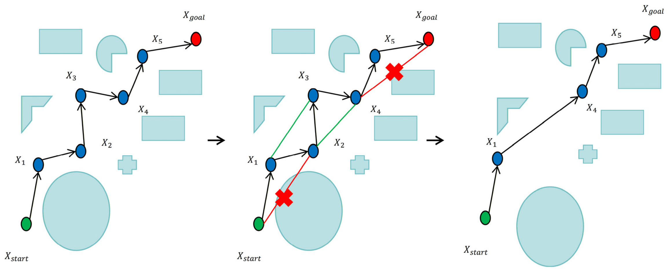
As illustrated in Figure 10, the global shortcutting stage tests collision-free connections between non-adjacent waypoints and uses dynamic programming to retain the connection sequence with the lowest cumulative path cost. The resulting path contains fewer redundant turns. Local iterative shortcutting then examines each remaining segment and removes intermediate waypoints only when the replacement segment satisfies the path-reduction and clearance conditions in Equation (18).

$${‖{\mathrm{x}}_{\mathrm{j}}-{\mathrm{x}}_{\mathrm{i}}‖}_2<\mathrm{\eta }{\displaystyle \sum _{\mathrm{k}=\mathrm{i}}^{\mathrm{j}-1}}{‖{\mathrm{x}}_{\mathrm{k}+1}-{\mathrm{x}}_{\mathrm{k}}‖}_2 \mathrm{a}\mathrm{n}\mathrm{d} \mathrm{d}({\mathrm{x}}_{\mathrm{i}},{\mathrm{x}}_{\mathrm{j}})>\mathrm{\sigma }$$

(18)

where $\mathrm{\eta }\in (\mathrm{0,1})$ is the path-reduction threshold, $\mathrm{d}({\mathrm{x}}_{\mathrm{i}},{\mathrm{x}}_{\mathrm{j}})$ denotes the minimum clearance along the shortcut segment, and $\mathrm{\sigma }$ is the safety margin. The refinement stops when no further valid shortcut can be found. This stage shortens the path while preserving collision safety.

4. Experimental Results and Analysis

To evaluate planning efficiency, path quality, search effort, and narrow-passage adaptability, comparative experiments were conducted in two geometric benchmark environments and a ROS-based manipulator simulation. HA-Bi-RRT* was compared with Bi-RRT, Bi-RRT*, RRT-Connect, RRT-Connect with bridge-test sampling, Skeleton-Guided RRT, Tunnel-RRT, and GDRRT*. These baselines represent bidirectional tree expansion, sampling-distribution enhancement, goal-distance guidance, and geometric guidance. All planners used the same collision-checking framework, maps, start–goal configurations, stopping limits, and matched random-seed sets.

4.1. Experimental Setup

All simulations were conducted on the same hardware platform to ensure a fair comparison. The computing platform was equipped with an Intel Core i5-12450H processor with a base frequency of 2.0 GHz and 16 GB of RAM. All algorithms were implemented in MATLAB R2024a and executed on Windows 11.

Two benchmark scenarios were used. Scenario 1 is the two-dimensional narrow-passage environment used to evaluate passage-entrance localization, traversal reliability, search efficiency, and path quality. Scenario 2 is the three-dimensional narrow-passage environment used to evaluate planning robustness and search efficiency under spatial constraints. A ROS-based 5-DOF manipulator simulation was additionally used to evaluate whether the mapped path could be converted into executable manipulator motion.

For fair comparison, all planners used the same obstacle maps, start–goal configurations, collision-checking resolution, maximum number of iterations, maximum number of generated nodes, and timeout threshold in each scenario. Algorithm-specific hyperparameters were fixed before the reported 100-trial test batches and then held constant during testing. The common experimental settings shared by all planners are summarized in Table 2, while the documented algorithm-specific settings are listed in

Table 3. Algorithm-specific hyperparameter settings.

Algorithm	Step Size	Goal Bias	Rewiring Radius	Special Parameters
Bi-RRT	2.0 cm	—	—	Connection threshold = 3.0 cm
Bi-RRT*	2.0 cm	0.10	4.0 cm	Neighbor radius = 6.0 cm; Connection threshold = 5.0 cm
RRT-Connect	2.0 cm	—	—	Connection threshold = 5.0 cm
RRT-Connect + Bridge Test	2.0 cm	—	—	Bridge-test probability = 0.45; bridge distance = 2.5 cm
Skeleton-Guided RRT	2.0 cm	0.10	—	Skeleton resolution = 0.25; skeleton bias = 0.75; σ = 0.35
Tunnel-RRT	2.0 cm	0.10	—	Tunnel bias = 0.50; radius = 10.0–35.0 cm; grow rate = 1.3
GDRRT*	2.0 cm	0.10	3.0–6.0 cm (S1); 2.5–5.0 cm (S2)	Near-goal distance = 8.0 cm; guide-box scale = 0.20; goal-connection radius = 5.0 cm
HA-Bi-RRT* (Ours)	2.0 cm	0.10–0.40	4.0 cm	Memory size = 20; window size = 10; boundary directions = 8; ${\mathrm{R}}_{\mathrm{b}\mathrm{a}\mathrm{s}\mathrm{e}}$$= 5.5 \mathrm{cm}; {\mathrm{f}}_{\mathrm{m}\mathrm{a}\mathrm{x}}$$= 6; {\mathrm{\tau }}_{\mathrm{s}}/{\mathrm{\tau }}_{\mathrm{f}}$= 0.65/0.35.

Note: Step size is reported in workspace units for the geometric benchmark scenarios. In the ROS simulation, the planned workspace path is mapped into the manipulator’s reachable region before inverse-kinematics conversion. For HA-Bi-RRT*, the goal-bias probability is adaptively adjusted within the range of 0.10–0.40 according to the recent extension success rate, while the initial value is set to 0.10 for all experiments. The GDRRT* implementation follows the goal-distance-based sampling formulation in [31] and uses the common stopping limits in Table 2. In Scenario 1, the goal-bias probability was 0.10, the rewiring radius was limited to 3.0–6.0 cm, the guide-advance fraction was 0.55, and the guide-box range was 2.0–8.0 cm. In Scenario 2, the goal-bias probability was also 0.10; the rewiring radius was limited to 2.5–5.0 cm, the guide-advance fraction was 0.45, and the guide-box range was 2.0–9.0 cm. Both settings used a nominal step size of 2.0 cm with an adaptive range of 0.8–3.0 cm, a near-goal distance of 8.0 cm, a guide-box scale of 0.20, and a goal-connection radius of 5.0 cm.

. The values listed in Table 2 are common hard caps; the shared quality-based early-stop rule is described in Section 3.1.

The HA-Bi-RRT* hyperparameters were empirically selected during preliminary testing and fixed before the formal repeated experiments. The base narrow-region sampling radius was set to ${\mathrm{R}}_{\mathrm{b}\mathrm{a}\mathrm{s}\mathrm{e}}$ = 5.5 cm to maintain localized exploration around detected bottleneck regions while providing sufficient coverage for escaping blocked extensions. The maximum consecutive-failure threshold was set to ${\mathrm{f}}_{\mathrm{m}\mathrm{a}\mathrm{x}}$ = 6 to prevent isolated extension failures from triggering excessive local adaptation. The success and failure thresholds were set to ${\mathrm{\tau }}_{\mathrm{s}\mathrm{u}\mathrm{c}\mathrm{c}\mathrm{e}\mathrm{s}\mathrm{s}}$ = 0.65 and ${\mathrm{\tau }}_{\mathrm{f}\mathrm{a}\mathrm{i}\mathrm{l}\mathrm{u}\mathrm{r}\mathrm{e}}$ = 0.35, respectively, creating a neutral interval that reduces frequent oscillation of the adaptive goal-bias probability. A window size of 10 was used to smooth short-term stochastic variations in extension outcomes, while a narrow-region memory size of 20 retained recent bottleneck information without excessive memory accumulation. Eight boundary-probing directions were adopted as a compromise between directional coverage and additional collision-checking cost. These settings were kept unchanged during the formal evaluation and are regarded as practical default values rather than globally optimal hyperparameters. The common 2.0 cm step size keeps expansion granularity comparable across planners. Rewiring radii are used only by planners that perform rewiring, whereas the remaining method-specific settings control each baseline’s intended sampling or geometric guidance mechanism. For HA-Bi-RRT*, the memory size and success-rate window limit the amount of recent feedback used by the adaptive sampler, and the boundary-direction count controls the angular resolution of local boundary probing. The algorithm-specific parameters listed in Table 3 were selected during preliminary validation and fixed before the formal 100-trial test batches. Parameter selection considered planning success rate, runtime, path cost, and search effort in the narrow-passage benchmark environments. The same final parameter settings were then retained throughout the reported comparison, and no parameter was adjusted according to the final test results. Because an exhaustive hyperparameter search over all baseline planners was not conducted, the reported settings should be regarded as documented practical configurations rather than globally optimal parameter combinations. The sensitivity of the two principal HA-Bi-RRT* parameters, $R_{base}$ and $f_{max}$, is examined separately in the section “Hyperparameter Sensitivity Analysis”.

The exploratory search ranges and exact number of preliminary validation scenes were not fully archived. These quantities therefore cannot be reconstructed reliably. Although the final configurations are documented, the incomplete preliminary-validation record prevents full reproduction of the parameter-selection process and verification of an equivalent tuning budget across planners. The reported comparisons therefore apply to the specified practical configurations; they do not establish performance rankings under globally optimized hyperparameters.

4.2. Evaluation Metrics and Statistical Protocol

The geometric benchmark comparison uses the five metrics reported in

Table 4. Quantitative comparison in Scenario 1 (100 independent trials).

Planner	Runtime, s Mean ± SD [95% CI]	Path Cost Mean ± SD [95% CI]	Success n/N (%; 95% CI)	Iterations Mean ± SD	Generated Nodes Mean ± SD	Holm-Adjusted p (Success)
Bi-RRT	0.319 ± 0.022 [0.314–0.324]	112.620 ± 3.836 [111.754–113.484]	74/100 (74%; 64.6–81.6)	2541.2 ± 222.2	777.4 ± 60.6	2.086 × 10−7
Bi-RRT*	2.810 ± 0.222 [2.763–2.856]	100.252 ± 3.544 [99.452–100.996]	79/100 (79%; 70.0–85.8)	2284.1 ± 195.8	550.0 ± 41.6	5.722 × 10−6
RRT-Connect	0.211 ± 0.019 [0.208–0.215]	113.795 ± 3.988 [113.022–114.570]	98/100 (98%; 93.0–99.4)	1608.3 ± 134.0	525.0 ± 43.1	1.000
RRT-Connect + Bridge Test	0.336 ± 0.026 [0.330–0.341]	110.712 ± 4.039 [109.945–111.503]	99/100 (99%; 94.6–99.8)	1438.2 ± 114.7	506.8 ± 38.6	1.000
Skeleton-Guided RRT	0.196 ± 0.014 [0.193–0.199]	104.413 ± 3.891 [103.648–105.183]	100/100 (100%; 96.3–100.0)	728.6 ± 70.2	385.4 ± 27.1	1.000
Tunnel-RRT	0.207 ± 0.016 [0.204–0.210]	103.329 ± 4.169 [102.547–104.141]	99/100 (99%; 94.6–99.8)	1536.3 ± 123.6	824.0 ± 69.7	1.000
GDRRT*	1.151 ± 0.222 [1.109–1.195]	94.609 ± 0.685 [94.481–94.748]	100/100 (100%; 96.3–100.0)	1795.5 ± 321.1	1073.8 ± 179.1	1.000
HA-Bi-RRT* (Ours)	0.186 ± 0.012 [0.184–0.188]	91.583 ± 2.501 [91.096–92.058]	100/100 (100%; 96.3–100.0)	1171.6 ± 75.8	656.0 ± 41.8	Reference

Note: All results are based on 100 independent trials. Runtime and path cost are calculated from successful trials only and are reported as mean ± SD with 95% confidence intervals. Iterations and generated nodes are summarized over all trials. Success n/N includes all trials and is accompanied by a Wilson 95% confidence interval. The final column reports Holm-adjusted p values from two-sided exact McNemar tests against HA-Bi-RRT*, reflecting the matched-seed design. Runtime and path cost are presented descriptively because the trial-level records needed for paired analyses are not currently available. For Skeleton-Guided RRT, the reported runtime excludes one-time skeleton construction and represents query-stage planning with a precomputed skeleton. Because preprocessing measurements are unavailable, total and amortized runtimes are not reported; timing comparisons are conditional on this boundary.

,

Table 5. Quantitative comparison in Scenario 2 (100 independent trials).

Planner	Runtime, s Mean ± SD [95% CI]	Path Cost Mean ± SD [95% CI]	Success n/N (%; 95% CI)	Iterations Mean ± SD	Generated Nodes Mean ± SD	Holm-Adjusted p (Success)
Bi-RRT	4.317 ± 0.239 [4.256–4.381]	213.635 ± 4.911 [212.356–214.844]	57/100 (57%; 47.2–66.3)	7552.9 ± 355.2	1813.9 ± 68.6	1.364 × 10−12
Bi-RRT*	4.820 ± 0.170 [4.787–4.853]	137.404 ± 1.420 [137.137–137.681]	99/100 (99%; 94.6–99.8)	9684.6 ± 279.9	3732.6 ± 89.2	1.000
RRT-Connect	0.589 ± 0.019 [0.585–0.593]	192.575 ± 1.982 [192.157–192.998]	86/100 (86%; 77.9–91.5)	3668.2 ± 90.4	1440.6 ± 33.6	0.000610
RRT-Connect + Bridge Test	0.717 ± 0.026 [0.712–0.722]	198.530 ± 2.693 [198.009–199.057]	100/100 (100%; 96.3–100.0)	3593.4 ± 126.6	1401.5 ± 33.6	1.000
Skeleton-Guided RRT	0.668 ± 0.023 [0.663–0.673]	159.645 ± 2.070 [159.203–160.067]	87/100 (87%; 79.0–92.2)	3737.1 ± 133.3	2041.6 ± 58.3	0.000977
Tunnel-RRT	1.454 ± 0.057 [1.443–1.465]	192.952 ± 2.879 [192.359–193.530]	93/100 (93%; 86.3–96.6)	7470.4 ± 296.0	3465.5 ± 109.5	0.046875
GDRRT*	0.695 ± 0.057 [0.675–0.716]	154.458 ± 2.899 [153.438–155.525]	28/100 (28%; 20.1–37.5)	5641.7 ± 315.5	3056.7 ± 249.0	2.965 × 10−21
HA-Bi-RRT* (Ours)	0.729 ± 0.011 [0.727–0.731]	118.842 ± 0.676 [118.708–118.973]	100/100 (100%; 96.3–100.0)	2556.3 ± 38.7	1418.4 ± 16.5	Reference

Note: All results are based on 100 independent trials. Runtime and path cost are calculated from successful trials only and are reported as mean ± SD with 95% confidence intervals. Iterations and generated nodes are summarized over all trials. Success n/N includes all trials and is accompanied by a Wilson 95% confidence interval. The final column reports Holm-adjusted p values from two-sided exact McNemar tests against HA-Bi-RRT*, reflecting the matched-seed design. Runtime and path cost are presented descriptively because the trial-level records needed for paired analyses are not currently available. For Skeleton-Guided RRT, the reported runtime excludes one-time skeleton construction and represents query-stage planning with a precomputed skeleton. Because preprocessing measurements are unavailable, total and amortized runtimes are not reported; timing comparisons are conditional on this boundary.

and

Table 6. Ablation results of HA-Bi-RRT* in Scenario 2.

Planner	Success Rate (%) [95% CI]	Runtime (s)	Path Cost	Iterations	Generated Nodes
Full HA-Bi-RRT*	100/100 (100%; 96.3–100.0)	0.691 ± 0.037 [0.684–0.698]	120.122 ± 5.102 [119.110–121.134]	2497.39 ± 175.00 [2462.67–2532.11]	1326.95 ± 92.00 [1308.70–1345.20]
–CB	77/100 (77%; 67.8–84.2)	0.853 ± 0.245 [0.798–0.908]	123.946 ± 6.976 [122.369–125.523]	3392.21 ± 430.00 [3294.99–3489.43]	1439.32 ± 138.00 [1408.12–1470.52]
–NRM	79/100 (79%; 70.0–85.8)	0.755 ± 0.042 [0.746–0.764]	120.155 ± 5.621 [118.900–121.410]	2523.46 ± 235.00 [2471.00–2575.92]	1294.65 ± 108.00 [1270.54–1318.76]
–CGS	91/100 (91%; 83.8–95.2)	0.710 ± 0.074 [0.695–0.725]	123.076 ± 7.155 [121.588–124.564]	2570.03 ± 248.00 [2518.45–2621.61]	1110.60 ± 86.00 [1092.71–1128.49]
–PR	100/100 (100%; 96.3–100.0)	0.684 ± 0.039 [0.676–0.692]	163.773 ± 13.003 [161.193–166.353]	2527.39 ± 218.00 [2484.14–2570.64]	1326.95 ± 106.00 [1305.92–1347.98]
Fixed goal bias	88/100 (88%; 80.2–93.0)	0.652 ± 0.044 [0.643–0.661]	123.005 ± 8.102 [121.291–124.719]	2440.70 ± 226.00 [2392.90–2488.50]	1229.65 ± 96.00 [1209.35–1249.95]

Note: CB, NRM, CGS, and PR denote cooperative breakthrough, narrow-region memory, centroid-guided sampling, and path refinement, respectively. The fixed-goal-bias variant disables adaptive goal-bias updating. Runtime and path cost are calculated from successful trials only; iterations and generated nodes are summarized over all trials. Success-rate parentheses report Wilson 95% confidence intervals based on 100 trials.

: planning success rate, path cost, runtime, generated nodes, and iterations. Joint-angle and clearance profiles are examined separately in the ROS simulation figures and are not included as columns in the benchmark tables.

The planning success rate measures the robustness of a planner in constrained spaces and is defined as the ratio of successful trials to the total number of independent trials:

$${\mathrm{P}}_{\mathrm{s}\mathrm{u}\mathrm{c}\mathrm{c}\mathrm{e}\mathrm{s}\mathrm{s}}={\displaystyle \frac{{\mathrm{N}}_{\mathrm{s}\mathrm{u}\mathrm{c}\mathrm{c}\mathrm{e}\mathrm{s}\mathrm{s}}}{{\mathrm{N}}_{\mathrm{t}\mathrm{o}\mathrm{t}\mathrm{a}\mathrm{l}}}}\times 100\%$$

(19)

where ${\mathrm{N}}_{\mathrm{s}\mathrm{u}\mathrm{c}\mathrm{c}\mathrm{e}\mathrm{s}\mathrm{s}}$ denotes the number of trials in which a collision-free path is successfully found from the start configuration to the goal configuration, and ${\mathrm{N}}_{\mathrm{t}\mathrm{o}\mathrm{t}\mathrm{a}\mathrm{l}}$ denotes the total number of independent trials conducted under the same experimental conditions.

The path cost is used to evaluate the quality of the generated path. For a successful trial, the path cost is computed as the cumulative Euclidean distance between consecutive waypoints:

$${\mathrm{L}}_{\mathrm{i}}={\sum }_{\mathrm{j}=1}^{{\mathrm{m}}_{\mathrm{i}}-1}\sqrt{{\left({\mathrm{x}}_{\mathrm{j}+1}^{(\mathrm{i})}-{\mathrm{x}}_{\mathrm{j}}^{(\mathrm{i})}\right)}^{\mathrm{T}}\left({\mathrm{x}}_{\mathrm{j}+1}^{(\mathrm{i})}-{\mathrm{x}}_{\mathrm{j}}^{(\mathrm{i})}\right)}$$

(20)

where ${\mathrm{x}}_{\mathrm{j}}^{(\mathrm{i})}$ denotes the (j)-th waypoint of the path generated in the (i)-th successful trial, and ${\mathrm{m}}_{\mathrm{i}}$ is the number of waypoints in that path. The average path cost over all successful trials is then calculated as

$$\overline{L}={\displaystyle \frac{1}{N_{success}}}{\sum }_{i=1}^{N_{success}}{L}_i$$

(21)

For the two-dimensional and three-dimensional benchmarks, path cost is reported in the coordinate unit of the Cartesian workspace. All path-cost values in Table 4, Table 5 and Table 6 are therefore workspace path lengths rather than joint-space trajectory costs.

Runtime evaluates the computational efficiency of successful planning trials and is defined as the elapsed time from the start of the planner call until the final path is returned. For HA-Bi-RRT*, this interval includes planner initialization, tree search, hierarchical geometric path refinement, and final path validation. The mean successful-trial runtime is calculated as

$$\overline{\mathrm{T}}={\displaystyle \frac{1}{{\mathrm{N}}_{\mathrm{s}\mathrm{u}\mathrm{c}\mathrm{c}\mathrm{e}\mathrm{s}\mathrm{s}}}}{\sum }_{\mathrm{i}=1}^{{\mathrm{N}}_{\mathrm{s}\mathrm{u}\mathrm{c}\mathrm{c}\mathrm{e}\mathrm{s}\mathrm{s}}}{\mathrm{T}}_{\mathrm{i}}$$

(22)

where ${\mathrm{T}}_{\mathrm{i}}$ denotes the runtime of the (i)-th successful trial. Failed trials are excluded from the runtime summary and represented through the success-rate metric. The reported mean is therefore based on successful trials only.

For Skeleton-Guided RRT, the reported runtime excludes one-time skeleton construction and represents query-stage planning with a precomputed skeleton. It is not an end-to-end timing measure from the raw map. The preprocessing time was not available for this analysis, so neither total runtime nor amortized runtime across repeated queries is quantified. The timing comparison is therefore conditional on the stated preprocessing boundary.

The number of generated nodes and the number of iterations are further recorded to evaluate the search complexity of each algorithm. Their average values are calculated as

$${\overline{\mathrm{N}}}_{\mathrm{n}\mathrm{o}\mathrm{d}\mathrm{e}\mathrm{s}}={\displaystyle \frac{1}{{\mathrm{N}}_{\mathrm{t}\mathrm{o}\mathrm{t}\mathrm{a}\mathrm{l}}}}{\sum }_{\mathrm{i}=1}^{{\mathrm{N}}_{\mathrm{t}\mathrm{o}\mathrm{t}\mathrm{a}\mathrm{l}}}{\mathrm{N}}_{\mathrm{n}\mathrm{o}\mathrm{d}\mathrm{e}\mathrm{s}}^{(\mathrm{i})}$$

(23)

$${\overline{\mathrm{N}}}_{\mathrm{i}\mathrm{t}\mathrm{e}\mathrm{r}}={\displaystyle \frac{1}{{\mathrm{N}}_{\mathrm{t}\mathrm{o}\mathrm{t}\mathrm{a}\mathrm{l}}}}{\sum }_{\mathrm{i}=1}^{{\mathrm{N}}_{\mathrm{t}\mathrm{o}\mathrm{t}\mathrm{a}\mathrm{l}}}{\mathrm{N}}_{\mathrm{i}\mathrm{t}\mathrm{e}\mathrm{r}}^{(\mathrm{i})}$$

(24)

where ${\mathrm{N}}_{\mathrm{n}\mathrm{o}\mathrm{d}\mathrm{e}\mathrm{s}}^{(\mathrm{i})}$ and ${\mathrm{N}}_{\mathrm{i}\mathrm{t}\mathrm{e}\mathrm{r}}^{(\mathrm{i})}$ denote the number of generated nodes and iterations in the (i)-th trial, respectively. A smaller number of nodes or iterations indicates that the planner can locate feasible regions more efficiently, which is particularly important in narrow-passage environments where invalid samples frequently occur.

To ensure fair comparison, all planners used the same obstacle maps, start–goal configurations, collision-checking resolution, maximum iterations, maximum generated nodes, and timeout threshold. They also used the same quality-based early-stop rule described in Section 3.1. Each planner was executed 100 times in each scenario using matched random-seed sets. Finding a first feasible path did not by itself end a run; the incumbent path could be improved until the shared quality rule or a shared hard limit was reached. HA-Bi-RRT* then applied its hierarchical path refinement before returning the final path. No additional planner-specific convergence tolerance was used. Planner-specific hyperparameters were fixed before testing, and the reported results apply to the settings documented in Table 2 and Table 3.

For metrics that require a feasible path, including path cost, only successful trials were included. Planning success rate was analyzed separately using binary success/failure outcomes.

Table 4 and Table 5 report mean ± SD and 95% confidence intervals from 100 independent trials. Runtime and path cost are computed over successful trials only; failed trials contribute to the success-rate calculation but are excluded from these continuous-metric summaries. Iterations and generated nodes are summarized over all trials, and Wilson 95% confidence intervals are reported for success rates. Pairwise success outcomes were compared using two-sided exact McNemar tests for the matched-seed design, with Holm adjustment across the seven comparisons against HA-Bi-RRT* separately within each scenario. HA-Bi-RRT* succeeded in all 100 trials in both scenarios, so the paired success tables were uniquely determined by the reported counts. Runtime and path cost are reported descriptively for successful trials only. The trial-level records required for paired analyses of these continuous outcomes are not currently available; therefore, no inferential significance claims are made for runtime or path cost.

Accordingly, continuous-metric comparisons are interpreted descriptively together with the repeated-trial distributions and confidence intervals.

4.3. Two-Dimensional Experiments

Scenario 1 was designed to evaluate planner robustness in a typical narrow-passage environment. This scenario contains constrained channels with small entrance regions, which significantly reduces the probability that uniformly sampled points fall inside feasible passage regions. Therefore, this scenario is more suitable for examining whether a planner can efficiently locate passage entrances and maintain stable tree growth inside confined regions.

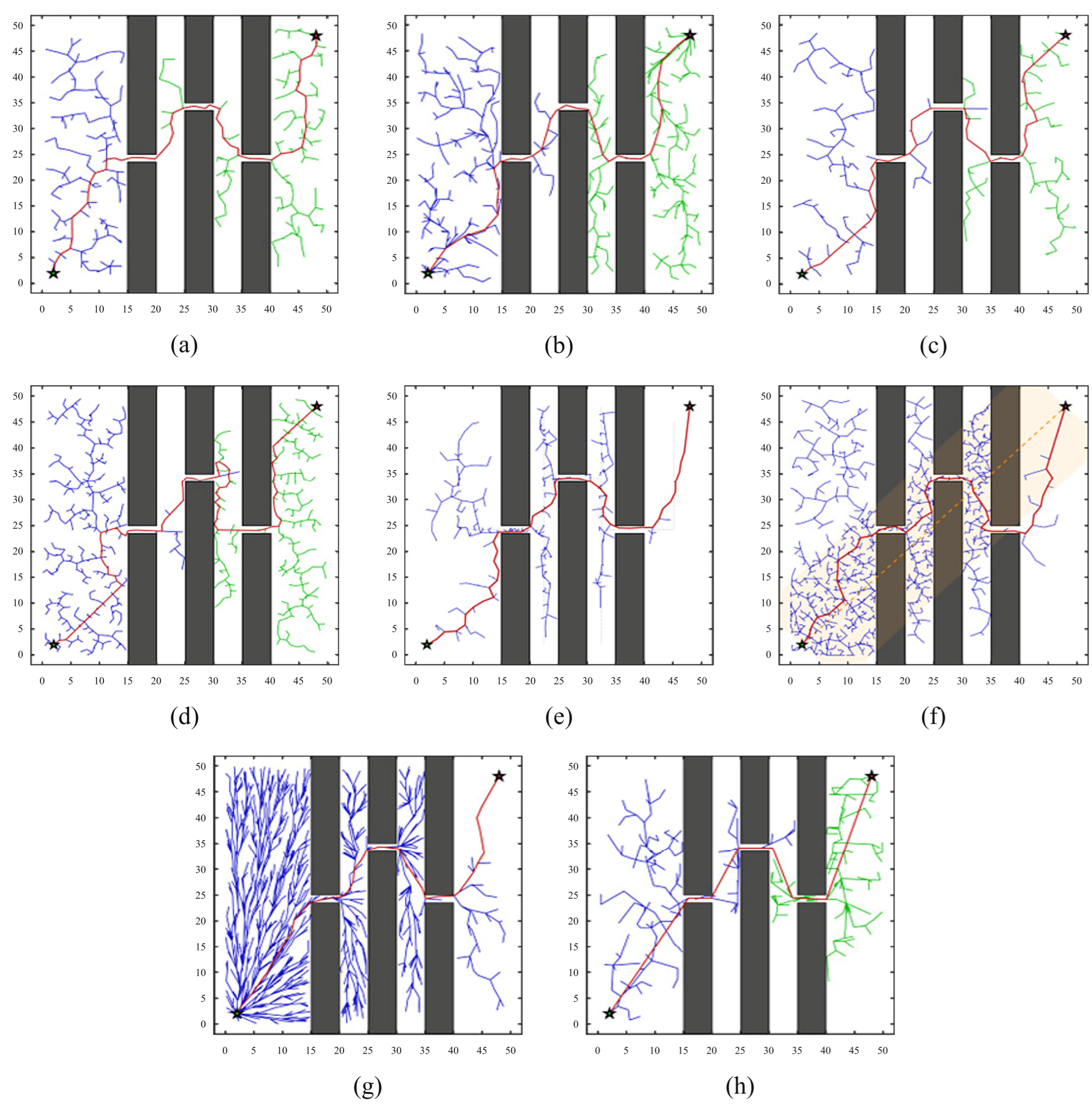
The representative planning results are shown in Figure 11, and the quantitative results are summarized in Table 4. As shown in Figure 11, the standard Bi-RRT* planner generates sparse tree branches near the passage entrance and frequently fails to extend deeply into the constrained channel. This phenomenon indicates that uniform sampling and conventional rewiring are insufficient for resolving the entrance-localization difficulty in narrow passages. RRT-Connect and its bridge-test variant improve connection efficiency, while Skeleton-Guided RRT and Tunnel-RRT provide stronger geometric guidance. However, these methods still produce longer paths or require additional structural assumptions.

HA-Bi-RRT* shows more stable passage penetration and generates a shorter path through the constrained channel. The cooperative breakthrough mechanism records blocked boundary nodes as bottleneck candidates and triggers boundary-following exploration, enabling the search tree to slide along obstacle contours rather than repeatedly discarding failed extensions. The recorded narrow-region memory further guides subsequent sampling toward critical constrained regions, thereby improving the probability of successful passage traversal.

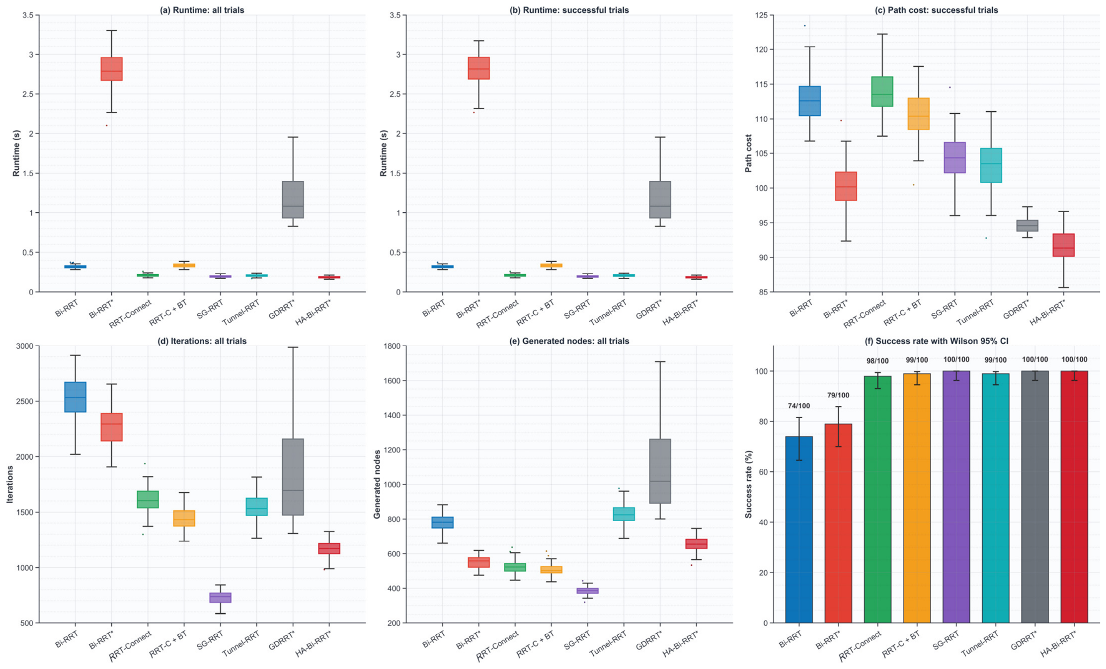
As shown in Table 4, HA-Bi-RRT* achieved a 100% success rate in the two-dimensional narrow-passage scenario. Relative to Bi-RRT*, the observed mean runtime decreased from 2.810 s to 0.186 s, and the observed mean path cost decreased from 100.252 to 91.583. Compared with GDRRT*, both planners achieved 100% success, while HA-Bi-RRT* had a lower observed mean runtime (0.186 s versus 1.151 s) and path cost (91.583 versus 94.609). HA-Bi-RRT* produced the lowest observed mean path cost among the compared planners. These results are consistent with more effective use of blocked boundary information during constrained-passage search. Path cost is calculated according to the definition in Section 4.2.

Figure 12 compares the performance distributions in Scenario 1, the two-dimensional narrow-passage experiment. HA-Bi-RRT* has the lowest runtime and path-cost distributions and requires fewer iterations than Bi-RRT*. Its generated-node count is not the smallest among the compared planners; therefore, the results indicate more effective sample placement rather than a uniform reduction in tree size.

4.4. Three-Dimensional Experiments and Ablation Study

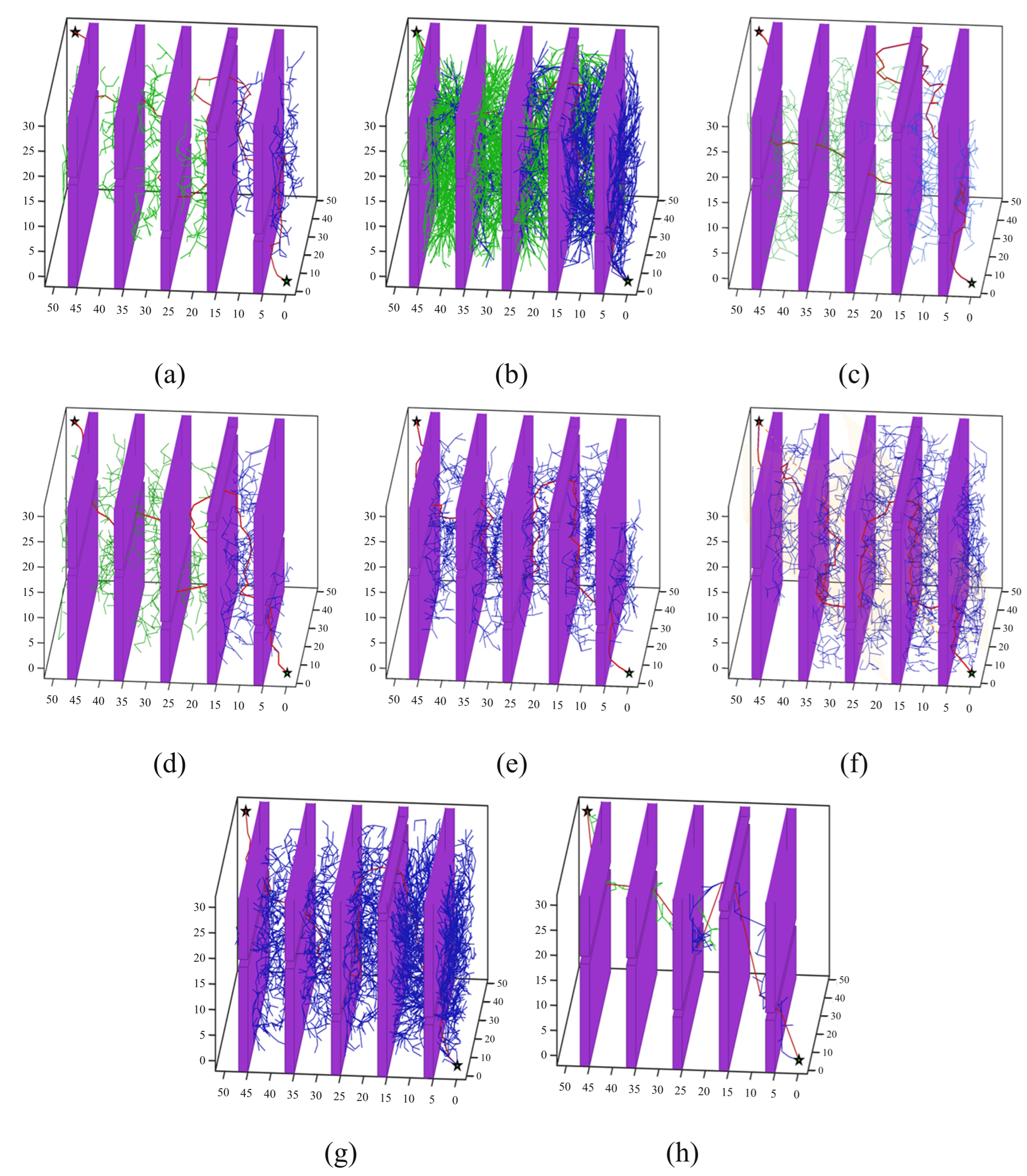
To further evaluate the robustness and search efficiency of the proposed planner in higher-dimensional constrained spaces, a three-dimensional narrow-passage environment was constructed as Scenario 2. The workspace size was set to 50 cm × 50 cm × 30 cm. Compared with the two-dimensional scenario, Scenario 2 contains more spatial constraints and dead-end regions, making it more challenging for sampling-based planners to locate feasible passages and maintain efficient tree growth.

The representative planning results are shown in Figure 13, and the quantitative comparison is summarized in Table 5.

Figure 13 shows that Bi-RRT and Bi-RRT* generate extensive search trees in the three-dimensional workspace, indicating that a large number of samples are spent in regions that do not directly contribute to a feasible solution. RRT-Connect and its bridge-test variant improve the connection speed, but their resulting paths remain relatively long in this constrained environment. Skeleton-Guided RRT and Tunnel-RRT provide additional geometric guidance, but their performance is still affected by the complexity of three-dimensional obstacle structures.

In contrast, HA-Bi-RRT* produces a more focused search pattern and avoids excessive exploration in dead-end regions. The cooperative breakthrough mechanism helps the planner identify constrained entrances from blocked expansion attempts, while the memory-guided adaptive sampling strategy concentrates samples around previously detected bottleneck regions. As a result, the proposed planner maintains stable passage traversal and generates a shorter path in the three-dimensional environment.

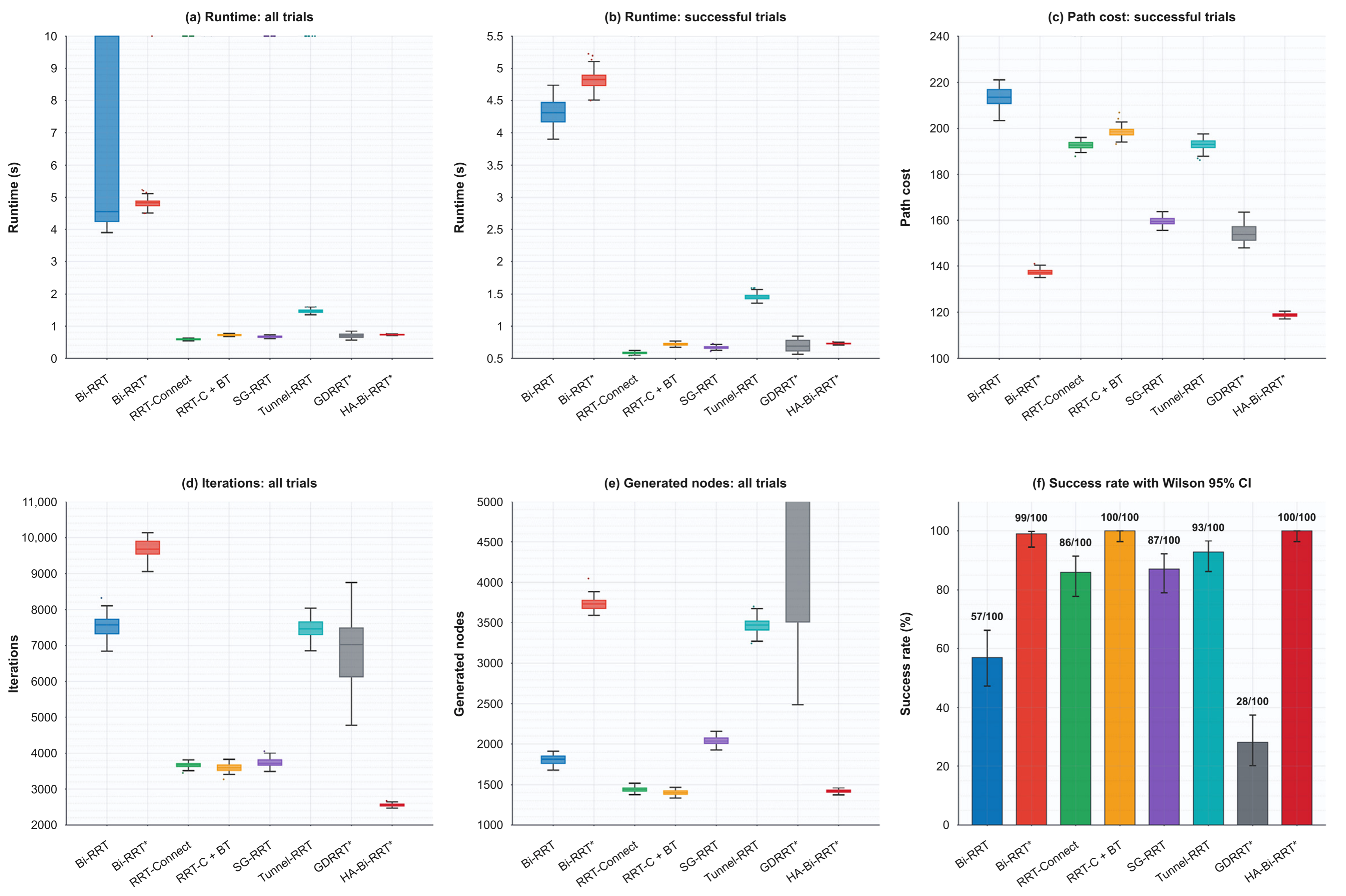
As shown in Table 5, HA-Bi-RRT* achieved a 100% success rate and the lowest observed mean path cost among the compared planners. Relative to Bi-RRT*, the observed mean runtime decreased from 4.820 s to 0.729 s, and the observed mean path cost decreased from 137.404 to 118.842. Although RRT-Connect with bridge-test sampling also achieved a 100% success rate, its observed mean path cost was higher. GDRRT* achieved a 28% success rate in this scenario; its runtime and path-cost summaries therefore describe only its successful trials and must be interpreted together with the success rate. These results describe the finite-budget performance of HA-Bi-RRT* in the tested three-dimensional narrow-passage environment.

Figure 14 presents the boxplot distributions of the compared planners in the three-dimensional narrow-passage scenario. HA-Bi-RRT* obtains the lowest path-cost distribution and requires fewer iterations than most baseline planners. Although RRT-Connect achieves a short runtime, its path-cost distribution is considerably higher, indicating that fast connection alone does not guarantee path quality in spatially constrained environments. The proposed planner achieves a better balance between search efficiency, robustness, and path compactness.

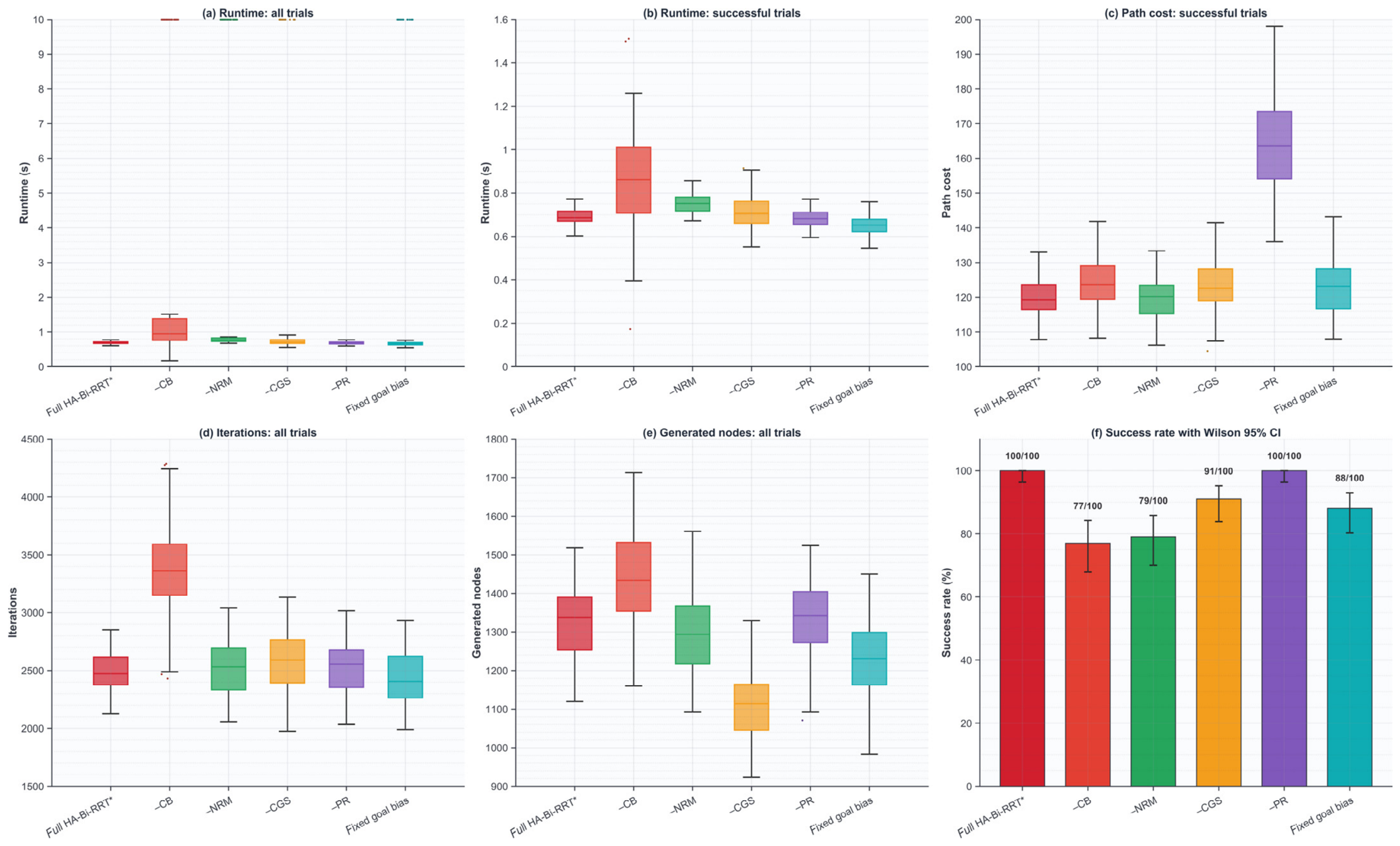
To identify the contribution of each component, an ablation study was conducted in Scenario 2, the three-dimensional narrow-passage setting described above. Six configurations were compared: the complete HA-Bi-RRT*, HA-Bi-RRT* without cooperative breakthrough (-CB), without narrow-region memory (-NRM), without centroid-guided sampling (-CGS), without path refinement (-PR), and a fixed-goal-bias variant in which adaptive goal-bias updating was disabled. All configurations used the same map, start–goal configuration, random seeds, and termination conditions.

The ablation study used a separate batch of 100 independent trials from the main comparison in Table 5. All ablation variants shared the same random seeds within that batch. This independent repetition explains why the full values in Table 6 are close to, but not numerically identical to, the HA-Bi-RRT* values in Table 5.

The fixed-goal-bias variant disables adaptive goal-bias updating while retaining the other HA-Bi-RRT* modules. It therefore isolates the contribution of the adaptive update mechanism under the settings of Scenario 2. The ablation study itself does not vary the base local sampling radius or the maximum failure threshold; their influence is evaluated separately in the hyperparameter sensitivity analysis presented in the section “Hyperparameter Sensitivity Analysis”. The success-rate thresholds are kept fixed throughout the reported experiments.

Table 6 shows that the complete planner and the -PR variant achieve a 100% success rate, whereas removing CB, NRM, and CGS reduces the success rate to 77%, 79%, and 91%, respectively. The fixed-goal-bias variant achieves an 88% success rate, compared with 100% for the complete planner; its observed mean runtime is slightly lower (0.652 s versus 0.691 s), but its observed mean path cost is higher (123.005 versus 120.122). These results indicate that adaptive goal-bias updating mainly supports planning reliability in the tested setting. Removing path refinement produces the largest path-cost increase, from 120.122 to 163.773. The -PR runtime is slightly lower because its post-processing stage is removed; this difference does not indicate better path quality. Figure 15 presents the distributions of runtime, path cost, iterations, and generated nodes over the repeated trials.

As shown in Figure 15, the complete HA-Bi-RRT* planner achieves balanced performance across the four metrics. Removing path refinement (-PR) markedly increases the path cost, confirming its role in improving solution quality. The -CB variant shows larger runtime fluctuations and requires more iterations and nodes, indicating that cooperative breakthrough stabilizes narrow-passage traversal. Although -CGS generates fewer nodes, its path cost and failure rate increase, suggesting that centroid-guided sampling supports directed and reliable exploration. The -NRM variant remains close to the complete planner in most metrics but has a lower success rate, showing that narrow-region memory mainly improves search robustness. The fixed-goal-bias result likewise indicates that adaptive goal-bias updating contributes primarily to reliability. Overall, these modules complement one another to improve path quality, search efficiency, and planning reliability.

Hyperparameter Sensitivity Analysis

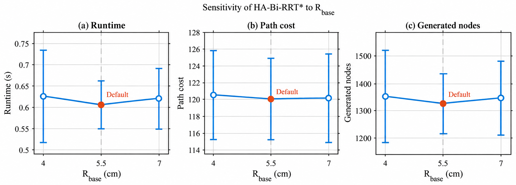
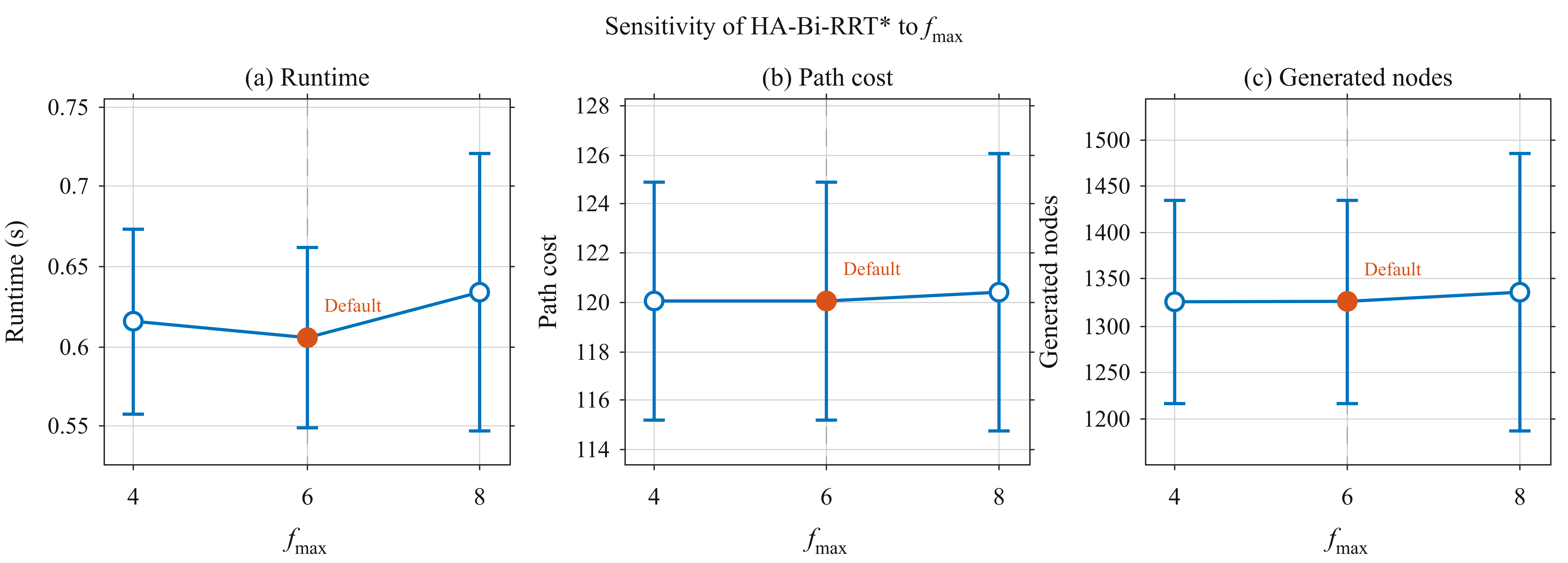
To further examine the robustness of the proposed planner with respect to key hyperparameters, a one-factor-at-a-time sensitivity analysis was conducted in Scenario 2. The base narrow-region sampling radius $R_{base}$ and the maximum consecutive-failure threshold $f_{max}$ were varied around their default settings, while all other algorithmic and experimental parameters were kept unchanged. Specifically, $R_{base}$ was evaluated at 4.0, 5.5, and 7.0 cm with $f_{max}=6$, whereas $f_{max}$ was evaluated at 4, 6, and 8 with $R_{base}=5.5$ cm. Each distinct parameter setting was evaluated over 100 independent trials using matched random seeds. Planning success rate, runtime, path cost, and generated nodes were recorded, and the continuous metrics are reported as mean ± standard deviation.

As shown in Figure 16, all three $R_{base}$ settings achieved a 100% planning success rate, indicating that HA-Bi-RRT* remains robust to moderate variations in the local narrow-region sampling radius. The tested settings produced relatively small changes in the continuous performance metrics. Among them, the default setting $R_{base}=5.5$ cm yielded the lowest mean runtime, path cost, and generated-node count. A smaller radius restricts local exploration around repeatedly blocked regions, whereas an excessively large radius may introduce unnecessary samples outside the most relevant bottleneck neighborhood. The selected value of 5.5 cm therefore provides a practical balance between local exploration coverage and computational efficiency.

As shown in Figure 17, varying $f_{max}$ from 4 to 8 produces only limited changes in runtime, path cost, and generated nodes, while all three settings maintain a 100% planning success rate. The substantial overlap of the error bars indicates that HA-Bi-RRT* is comparatively insensitive to the maximum consecutive-failure threshold within the tested range. The default value $f_{max}=6$ provides stable planning performance while avoiding either overly rapid or overly delayed enlargement of the local sampling region.

Overall, the sensitivity analysis shows that HA-Bi-RRT* does not exhibit abrupt performance degradation under moderate variations of $R_{base}$ and $f_{max}$. The default settings $R_{base}=5.5$ cm and $f_{max}=6$ are therefore retained as practical operating values for the experiments in this study. These results indicate local parameter robustness within the tested ranges rather than globally optimal hyperparameter values.

4.5. ROS-Based Manipulator Simulation

The three-dimensional geometric benchmark evaluates search efficiency and workspace path quality but does not by itself establish manipulator executability. A ROS-based simulation was therefore constructed using MATLAB R2024a, ROS Noetic, MoveIt 1, and RViz (default versions shipped with ROS Noetic). MATLAB generated the Cartesian workspace path, while the ROS bridge performed path transmission, inverse-kinematics conversion, joint-trajectory generation, and visual execution verification.

4.5.1. Simulation Setup and Task Definition

The MATLAB planning workspace was set as a three-dimensional space with a size of 50 by 50 by 30. The start point was set to 2.0, 2.0, 2.0, and the goal point was set to 48.0, 48.0, 26.0. These two points form a long-distance planning task from a low-position region to a high-position target region. The detailed planner parameters are consistent with those listed in the previous tables and are not repeated in this section.

After generation in MATLAB, the path was transmitted through /matlab_rrt_ik_path_x, while the obstacle representation was displayed through /matlab_obstacles_marker. Because the MATLAB planning domain exceeded the reachable region of the Dofbot manipulator, the path and obstacle representation were mapped into the execution workspace before inverse-kinematics conversion. This mapping belongs to the execution layer rather than to the HA-Bi-RRT* search. The same coordinate transformation was applied to both the planned path and the obstacle representation, preserving their relative spatial relationships, while the absolute obstacle dimensions, path length, and clearance were scaled proportionally in the execution workspace.

Because scaling changes absolute path length and clearance, quantitative path-cost comparisons are based on the original benchmark workspace; the mapped ROS path is used to evaluate reachability and execution feasibility.

The Python bridge (Version 6.2.0.341, COMSOL AB, Stockholm, Sweden) subscribed to the mapped path and called the Dofbot inverse-kinematics service /dofbot_kinemarics for each waypoint. Valid joint targets were then passed to MoveIt for joint-trajectory generation under the configured robot model, joint-limit constraints, and collision-checking framework. In RViz, the obstacles were displayed as solid markers and the mapped end-effector path was shown as a red line.

The HA-Bi-RRT* collision model verifies the inflated Cartesian workspace path of the end effector. It does not, by itself, constitute an independent collision certificate for each manipulator link. The present ROS experiment therefore demonstrates workspace-to-joint conversion and execution feasibility under the configured pipeline; it should not be interpreted as proof of globally optimal joint-space motion or certified whole-arm clearance.

4.5.2. Execution Results and Trajectory Analysis

The ROS-based simulation completed the mapped waypoint sequence. For each waypoint, the bridge obtained an inverse-kinematics solution and passed the corresponding joint target to MoveIt. The result shows that the workspace path could be converted into continuous manipulator motion in the modeled environment under the common IK and trajectory-generation pipeline.

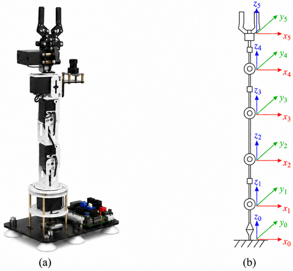
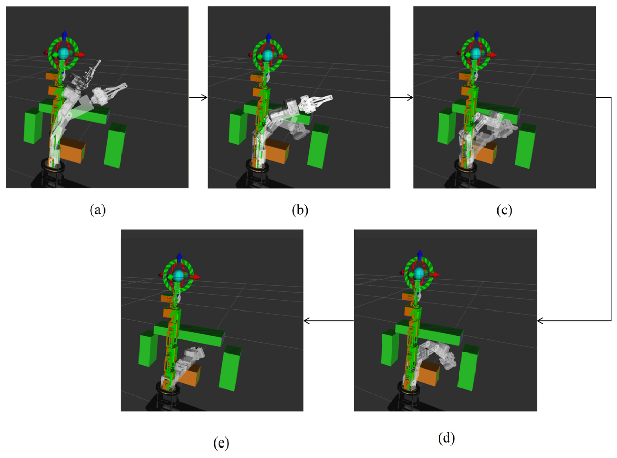
Figure 18 shows the simulated execution sequence of the 5-DOF Dofbot manipulator. The manipulator starts from the initial configuration, approaches the constrained passage, passes through the reserved opening between the obstacles, and finally reaches the target region. The red line represents the mapped end-effector trajectory, while the solid obstacles represent the local constrained environment.

The sequence shows that the mapped workspace path can guide the manipulator through the constrained region in the tested ROS model. It therefore supports execution feasibility for the laboratory sorting workflow, rather than direct joint-space optimality or general industrial deployment.

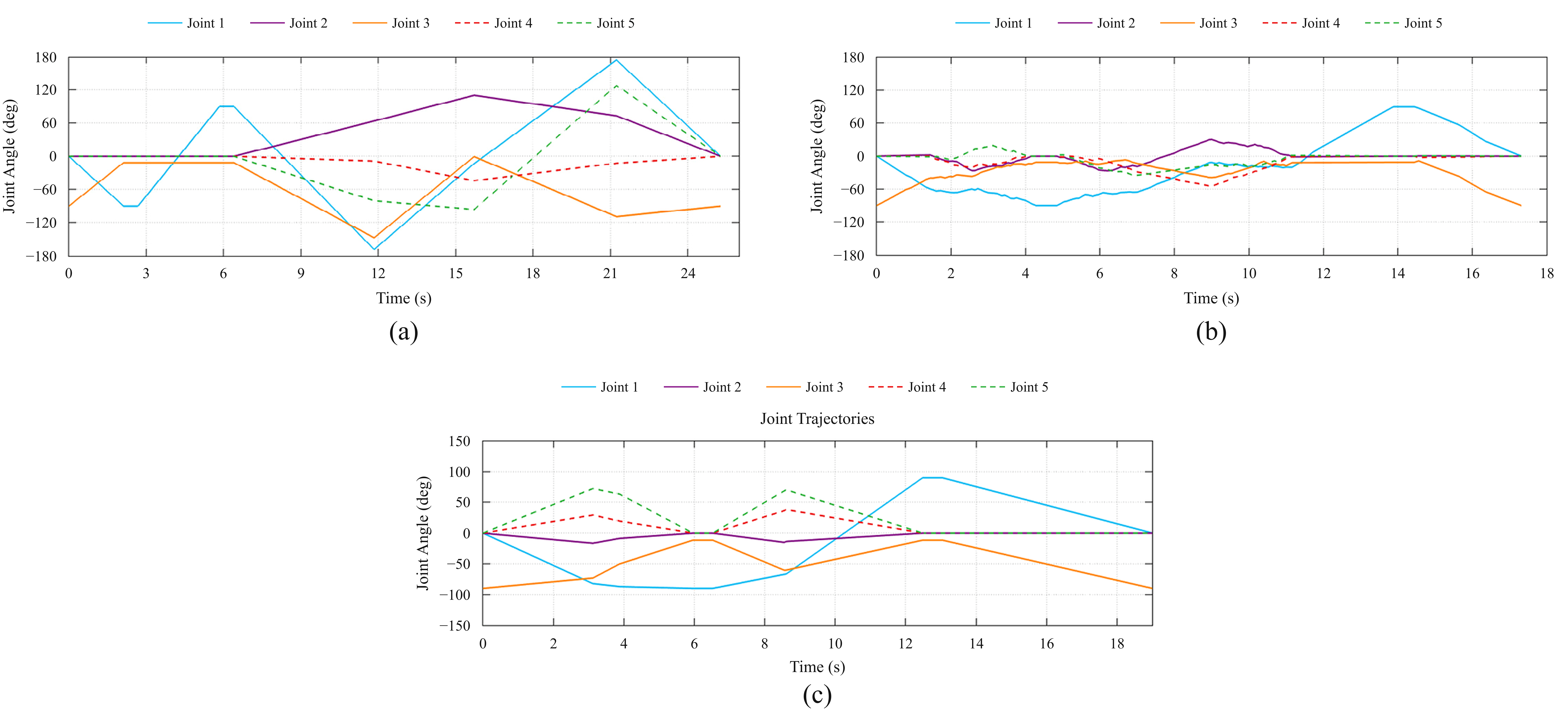
Figure 19 compares the resulting joint-angle profiles after the workspace paths from the three planners were mapped, converted by inverse kinematics, and processed by MoveIt. The HA-Bi-RRT* case exhibits fewer abrupt variations under this common pipeline. This observation is consistent with a workspace path containing fewer redundant waypoints, but the profiles also depend on IK branch selection and MoveIt interpolation. The figure therefore supports relative execution continuity in this test and should not be interpreted as evidence that HA-Bi-RRT* directly optimizes joint-space trajectories.

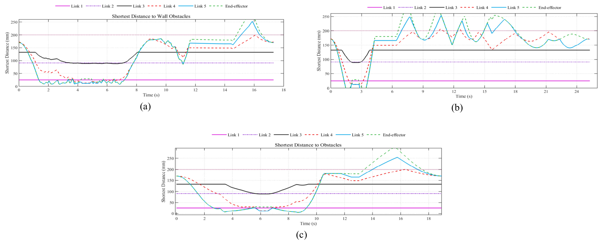
Figure 20 shows the end-effector minimum-clearance profiles after workspace mapping. In this test, the HA-Bi-RRT* case exhibits less repeated clearance fluctuation than the two baselines. The profiles are affected by mapping and the common IK/MoveIt pipeline and do not measure the clearance of every manipulator link. They are therefore reported as descriptive execution evidence rather than proof of whole-arm clearance superiority.

4.6. Physical Manipulator Experiments

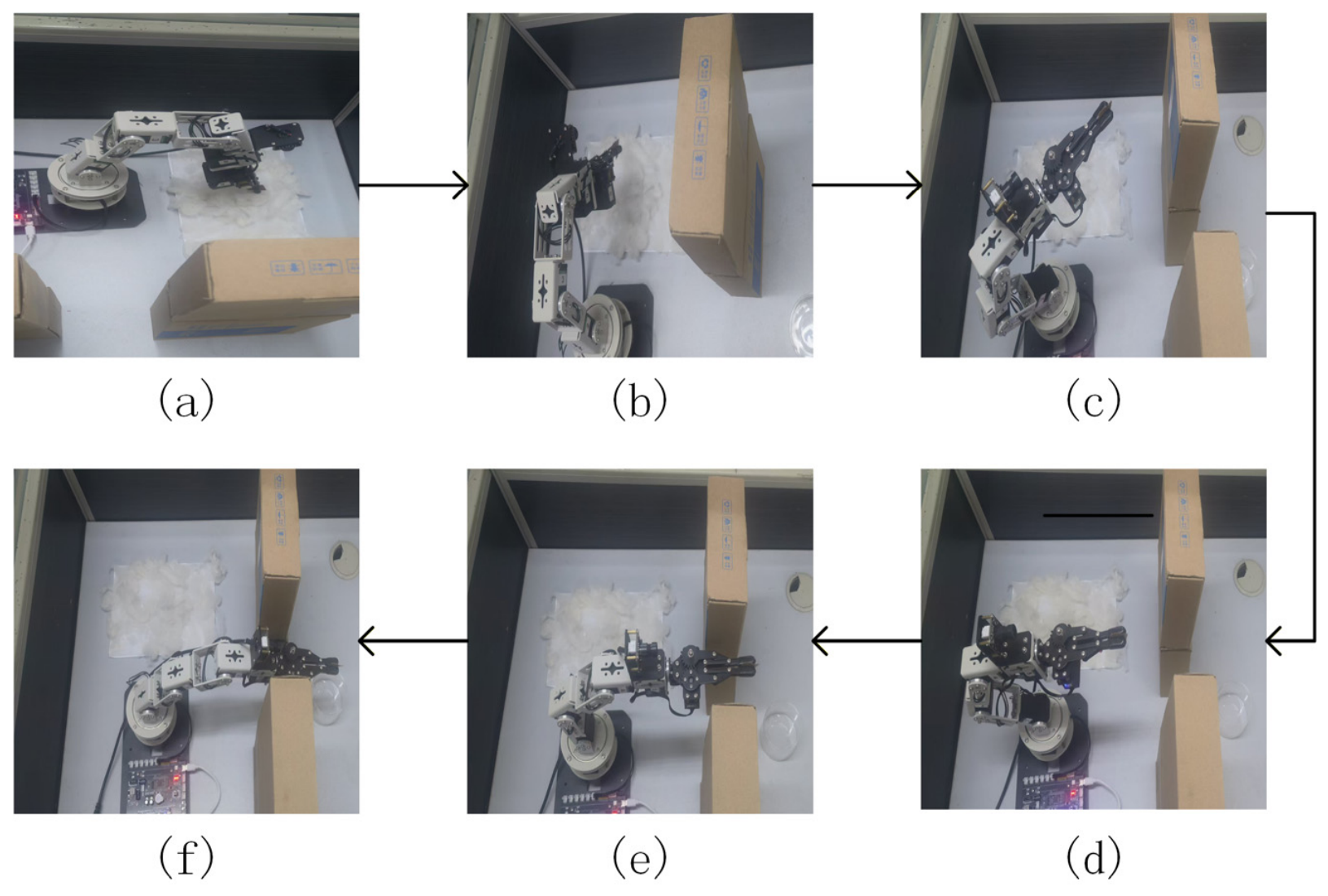
To evaluate the practical feasibility of the proposed planner, physical foreign-matter removal experiments were conducted using a 5-DOF DOFBOT manipulator. A laboratory-scale wool–cashmere sorting workspace was constructed, in which two cardboard barriers formed a constrained passage between the manipulator and the target region. In the original configuration, a leaf impurity on the wool–cashmere sample served as the representative target.

The experimental task consisted of four stages: approaching the passage entrance, traversing the constrained region, grasping the impurity, and transferring it to the designated collection area. Within each configuration, all compared planners used the same obstacle layout, target position, initial manipulator configuration, goal configuration, joint-motion parameters, and termination conditions.

Skeleton-Guided RRT, RRT-Connect with bridge-test sampling, and HA-Bi-RRT* were each independently tested 20 times. A trial was successful only when the manipulator completed the entire task without colliding with the barriers, dropping the impurity, exceeding the planning timeout, or failing to reach the target configuration. Task completion time was measured from the start of planning to the completion of impurity placement and included path generation, manipulator motion, grasping, and transfer. Mean completion time in

Table 7. Physical task-completion time with percentile-bootstrap 95% confidence intervals and success rate with Wilson 95% confidence intervals.

Configuration	Planner	Mean Successful-Trial Completion Time (s) [95% CI]	Successful Trials/Total; Rate [95% CI]
	Skeleton-Guided RRT	31.2 [28.4–34.7]	16/20 (80%; 58.4–91.9)
typical narrow passage	RRT-Connect with bridge-test sampling	27.1 [24.3–30.2]	15/20 (75%; 53.1–88.8)
	HA-Bi-RRT* (Ours)	25.9 [23.1–28.4]	19/20 (95%; 76.4–99.1)
	Skeleton-Guided RRT	36.9 [32.6–41.5]	11/20 (55%; 34.2–74.2)
Narrower passage (90% of original width) with an additional obstacle	RRT-Connect with bridge-test sampling	30.8 [26.7–35.1]	7/20 (35%; 18.1–56.7)
	HA-Bi-RRT* (Ours)	29.1 [25.2–33.0]	13/20 (65%; 43.3–81.9)

was calculated from successful trials only. Its 95% confidence interval was obtained from the 2.5th and 97.5th percentiles of a nonparametric bootstrap distribution formed by resampling successful-trial times within each planner and configuration. Success-rate intervals were calculated by the Wilson score method using all 20 trials. Because the available experiment log does not separately document whether Skeleton-Guided RRT skeleton construction occurred within this interval, Table 7 is not used to support an end-to-end timing comparison from raw-map preprocessing.

Skeleton-Guided RRT and RRT-Connect with bridge-test sampling were selected as representative geometry-guided and narrow-passage-biased sampling baselines, respectively, and both were executable through the same hardware interface. Limiting the physical comparison to these two baselines reflects the scope of the laboratory feasibility study; broader hardware comparisons remain future work.

Figure 21 presents six representative frames from a successful experiment using HA-Bi-RRT*. The manipulator first approached the narrow-passage entrance and adjusted its joint configuration to avoid the surrounding barriers. It then traversed the constrained region, reached the wool–cashmere sample, grasped the leaf impurity, and transferred it to the collection area. No collision with the barriers was observed during this representative execution sequence.

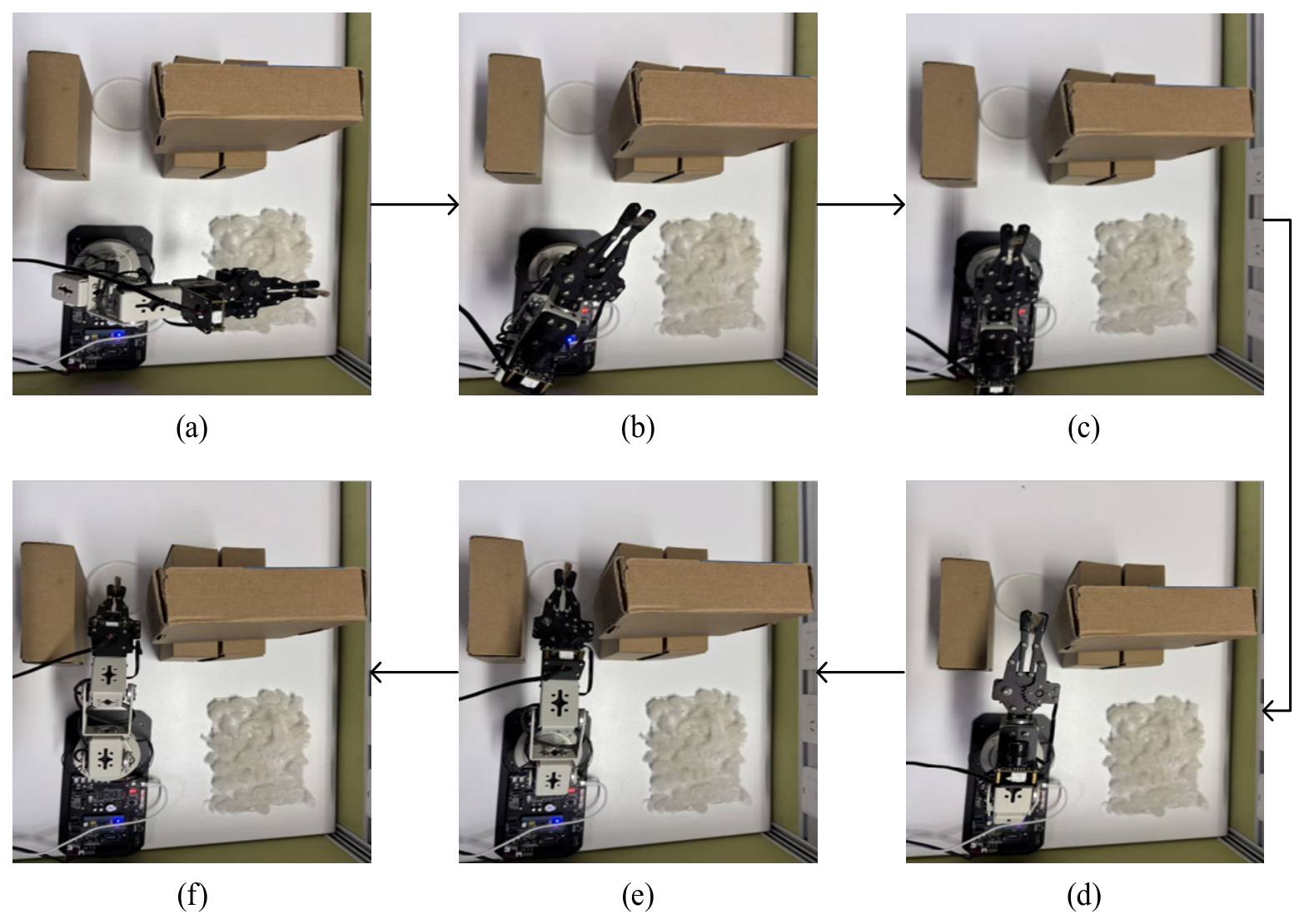
To further evaluate the planner under a more constrained physical configuration, an additional experiment was conducted by reducing the passage width to 90% of that in the original setup and introducing an additional obstacle near the narrow-passage region. This modification reduces the available maneuvering space and increases the difficulty of passage traversal. The manipulator platform, task procedure, success criteria, and evaluation protocol were otherwise kept unchanged. The representative target was changed from a leaf impurity in the original configuration to a coarse hemp-rope fragment in the additional configuration.

Each planner was evaluated over 20 independent trials under this additional configuration. The representative physical execution sequence is shown in Figure 22.

Figure 22. Representative physical execution sequence of the coarse hemp-rope fragment grasping and transfer task in the narrower-passage configuration (90% of the original passage width) with an additional obstacle, using the HA-Bi-RRT* planner: (a) end-effector near the sample region; (b) arm reconfiguration; (c) gripper alignment toward the passage between the obstacles; (d) approach toward the collection area; (e) gripper positioning near the collection area; and (f) final manipulator configuration at the collection area.

Figure 22. Representative physical execution sequence of the coarse hemp-rope fragment grasping and transfer task in the narrower-passage configuration (90% of the original passage width) with an additional obstacle, using the HA-Bi-RRT* planner: (a) end-effector near the sample region; (b) arm reconfiguration; (c) gripper alignment toward the passage between the obstacles; (d) approach toward the collection area; (e) gripper positioning near the collection area; and (f) final manipulator configuration at the collection area.

Table 7 summarizes the physical experimental results under the two narrow-passage configurations. In the typical narrow-passage configuration, HA-Bi-RRT* successfully completed 19 of 20 trials, corresponding to a 95% success rate with a Wilson 95% confidence interval of 76.4–99.1%, and achieved the lowest mean successful-trial completion time of 25.9 s. Skeleton-Guided RRT completed 16 of 20 trials (80%; 58.4–91.9%), whereas RRT-Connect with bridge-test sampling completed 15 of 20 trials (75%; 53.1–88.8%).

In the more constrained configuration, the passage width was reduced to 90% of the original value and an additional obstacle was introduced near the narrow-passage region. The success rates of all three planners decreased under the second experimental condition. Because this condition involved both a narrower passage with an additional obstacle and a different representative impurity target, the observed performance differences should be interpreted as results under the combined experimental variation rather than being attributed solely to geometric narrowing.

Skeleton-Guided RRT achieved 11 successes in 20 trials (55%; 34.2–74.2%), while RRT-Connect with bridge-test sampling achieved seven successes (35%; 18.1–56.7%). HA-Bi-RRT* achieved 13 successes (65%; 43.3–81.9%) and retained the lowest mean successful-trial completion time of 29.1 s, compared with 36.9 s for Skeleton-Guided RRT and 30.8 s for RRT-Connect with bridge-test sampling.

The additional experiment therefore provides further laboratory-scale evidence that HA-Bi-RRT* can maintain comparatively favorable task-execution performance under moderate passage narrowing and local obstacle-layout variation. Under the narrower configuration, its observed mean successful-trial completion time was approximately 21.1% lower than that of Skeleton-Guided RRT and 5.5% lower than that of RRT-Connect with bridge-test sampling, while its success rate remained 10 and 30 percentage points higher, respectively. These comparisons are descriptive and should not be interpreted as statistically significant effects because only 20 physical trials were conducted per method in each configuration.

The physical experiments demonstrate that HA-Bi-RRT* workspace paths can be executed by a laboratory-scale 5-DOF manipulator for representative impurity removal from wool–cashmere material in two laboratory configurations. The original narrow-passage configuration used a leaf impurity; the additional configuration used a coarse hemp-rope fragment, a passage width reduced to 90% of the original value, and an additional obstacle. These experiments remain limited to one manipulator platform, two representative impurity types, and 20 trials per method in each configuration.

Therefore, the results establish laboratory prototype feasibility and provide preliminary evidence of adaptability to moderate geometric variation, rather than demonstrating general performance across diverse manipulator structures, impurity types, or industrial workcell conditions. Broader validation with additional target positions, obstacle arrangements, passage geometries, impurity types, and higher-DOF manipulators remains necessary.

5. Conclusions

This paper proposed HA-Bi-RRT*, a failure-informed adaptive bidirectional planner for narrow-passage motion planning of fiber-sorting manipulators. The key idea is to reuse collision-induced extension failures as informative cues for narrow-passage localization rather than simply discarding them as invalid samples. The proposed planner integrates three main components: a cooperative breakthrough mechanism, memory-guided hybrid adaptive sampling, and hierarchical path refinement. The cooperative breakthrough mechanism records blocked boundary nodes as bottleneck candidates and guides subsequent boundary-following expansion. The hybrid adaptive sampler switches among goal-biased, centroid-guided, and narrow-region sampling according to recent tree-growth feedback, while the path-refinement module removes redundant waypoints and improves path compactness.

Comparative experiments in Scenario 1 (two-dimensional narrow passage) and Scenario 2 (three-dimensional narrow passage) demonstrated favorable finite-budget performance of the proposed planner. In Scenario 1, HA-Bi-RRT* increased the success rate from 79% to 100% relative to Bi-RRT*, reduced the mean runtime from 2.810 s to 0.186 s, and reduced the mean path cost from 100.252 to 91.583. In Scenario 2, HA-Bi-RRT* achieved a 100% success rate, a mean runtime of 0.729 s, and a mean path cost of 118.842. The ablation study further showed that the cooperative breakthrough mechanism, narrow-region memory, and adaptive goal-bias updating mainly contribute to planning reliability, whereas hierarchical path refinement primarily reduces path cost.

The hyperparameter sensitivity analysis showed that moderate variations of the base narrow-region sampling radius (R_base) and the maximum consecutive-failure threshold (f_max) did not cause abrupt performance degradation in Scenario 2. The default settings R_base = 5.5 cm and f_max = 6 provided stable performance within the tested ranges and were therefore retained as practical operating values. These results indicate local robustness of the selected settings rather than globally optimal hyperparameter values.

The ROS simulation further demonstrated that the Cartesian workspace path generated by HA-Bi-RRT* can be mapped into the reachable region of the Dofbot manipulator, converted into joint targets through inverse kinematics, and executed within the configured MoveIt environment. The resulting joint-angle and end-effector-clearance profiles are descriptive outcomes of the complete workspace mapping, inverse-kinematics, and MoveIt execution pipeline; they should not be interpreted as evidence of direct joint-space optimality or certified all-link clearance.

The physical experiments further evaluated the planner under two laboratory-scale geometric configurations. In the typical narrow-passage configuration, HA-Bi-RRT* achieved 19 successful trials out of 20, corresponding to a 95% success rate, with a mean successful-trial completion time of 25.9 s. In the more constrained configuration, the passage width was reduced to 90% of the original value and an additional obstacle was introduced near the narrow-passage region. The combined changes in passage geometry, obstacle layout, and representative target were accompanied by lower success rates for all three planners. Nevertheless, HA-Bi-RRT* retained the highest observed success rate of 65% (13/20) and the lowest mean successful-trial completion time of 29.1 s among the tested methods. The additional configuration therefore provides further laboratory-scale evidence of comparatively favorable execution performance in the second tested setting. The simultaneous changes mean that the difference between configurations cannot be attributed to passage width alone.

This study remains limited to static environments, two laboratory-scale physical configurations, one 5-DOF manipulator, two representative impurity types, and the reported hyperparameter settings. Although the workspace-planning formulation is not explicitly tied to the number of manipulator joints, its executability and performance on higher-DOF manipulators have not yet been experimentally established. Moreover, the current physical experiments are intended to demonstrate laboratory prototype feasibility rather than industrial applicability. Future work will investigate dynamic obstacle avoidance, online replanning with visual feedback, full-link collision verification, higher-DOF manipulators, broader sensitivity analysis covering additional hyperparameters and planning environments, and more extensive physical experiments involving varied target positions, passage geometries, obstacle arrangements, impurity types, and workcell layouts.