Design and Experimental Validation of an Adaptive Robust Control Algorithm for a PAM-Driven Biomimetic Leg Joint System

Abstract

Biomimetic quadruped robots, inspired by the musculoskeletal systems of animals, employ pneumatic artificial muscles (PAMs) as compliant actuators to achieve flexible, efficient, and adaptive locomotion. This study focuses on a pneumatic artificial muscle (PAM)-driven biomimetic leg joints system. First, its kinematic and dynamic models are established. Next, to address the challenges posed by the strong nonlinearities and complex time-varying uncertainties inherent in PAMs, an adaptive robust control algorithm is proposed by employing the Udwadia controller. Rigorous theoretical analysis of the adaptive robust control algorithm is verified via the Lyapunov stability method. Finally, numerical simulations and hardware experiments are conducted on the PAM-driven biomimetic leg joints system under desired trajectories, where the adaptive robust control algorithm is systematically compared with three conventional control algorithm to evaluate its control performance. The experimental results show that the proposed controller achieves a maximum tracking error of within 0.05 rad for the hip joint and within 0.1 rad, highlighting its strong potential for practical deployment in real-world environments.

1. Introduction

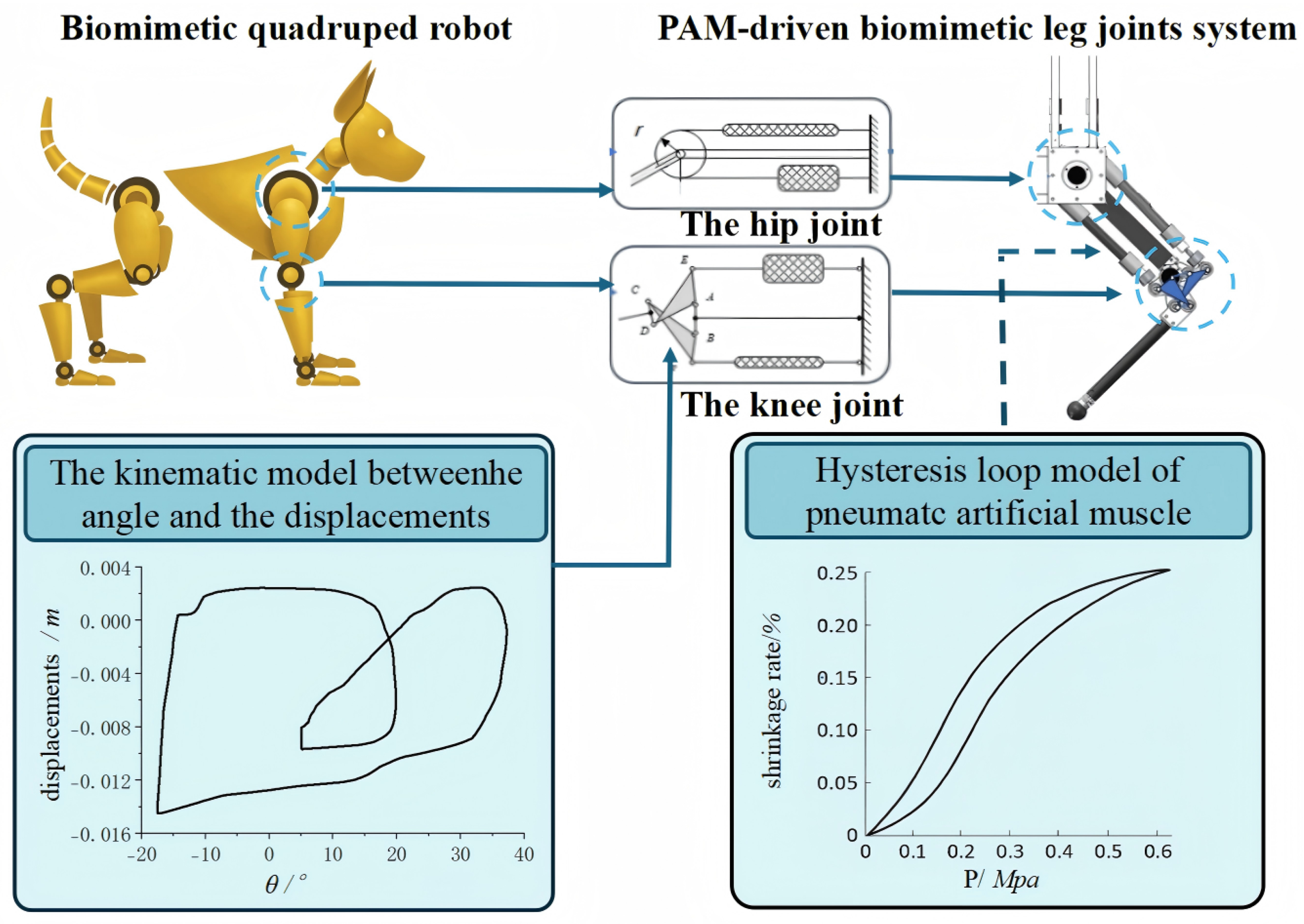
In recent years, biomimetic robots have emerged as a promising frontier in legged locomotion, offering new possibilities for achieving agile, robust, and energy-efficient movement in complex environments [1]. Unlike conventional rigid actuators, pneumatic artificial muscles (PAMs) offer a high power-to-weight ratio, inherent compliance, and are safe and lightweight, which is particularly important for energy-efficient movement. As illustrated in Figure 1, the canine-inspired knee joint does not follow a fixed-axis rotation but exhibits a variable instantaneous center of rotation (ICR) [2], which is realized via a four-bar linkage mechanism to achieve variable-center kinematics and enhanced mechanical flexibility. To further mimic the softness and adaptability of biological muscles, PAMs are employed to actuate both the hip and knee joints [3], enabling compliant and natural movement patterns. However, PAMs exhibit pronounced nonlinear and hysteretic behaviors [4,5]. For pneumatic artificial muscles, the hysteresis is mainly manifested as lag in the contraction force length relationship and lag in the pressure length relationship. In addition, the variable ICR structure introduces strong kinematic nonlinearities, which are specifically reflected in the nonlinear mapping between the joint rotation angle and the PAM end displacement. These nonlinear effects, together with modeling uncertainties, external disturbances, and payload variations, render the system dynamics strongly nonlinear and time-varying. However, the Udwadia controller computes only the nominal joint torques of the model and does not account for unknown model uncertainties, thereby posing substantial challenges for accurate modeling and high-precision motion control in PAM-driven biomimetic leg-joint systems.

To overcome these challenges, advanced control systems such as sliding mode control (SMC) [6], adaptive control [7,8], and robust control [9] can be employed. These methods have been extensively developed to address the nonlinearities, uncertainties, and time-varying disturbances in mechanical systems, effectively suppressing their adverse effects while improving tracking accuracy and system robustness. Among the various promising techniques explored in related studies, it is noteworthy that Udwadia adopted a new perspective on desired trajectories [10] and proposed a novel Udwadia controller [11]. The controller inputs required to enforce the desired trajectories are obtained in a fully explicit closed form, and the associated computations reduce to simple matrix multiplications and additions, thereby avoiding heavy analytical derivations and numerical optimization. However, the Udwadia controller only computes the nominal joint torques of the model and does not account for unknown model uncertainties. In practical applications, such uncertainties are inevitable and can significantly degrade system performance if not properly handled. To address this issue, Chen et al. employed the Udwadia controller and further developed an adaptive robust control scheme in [12], contributing to the theoretical advancement of this methodology. Since then, numerous studies have extended the Udwadia controller to uncertain nonlinear systems. For instance, Chen et al incorporated the Udwadia controller into a model-based robust controller to address modular joint dynamics in dual-arm robot [13], while Huang et al. proposed an adaptive robust strategy for uncertain inverted pendulum systems within the same framework [14]. In addition, robust Udwadia controller have been reported for systems operating under uncertainties [15,16]. Beyond electromechanical systems, Chen et al also proposed a three-level interaction force control architecture for a hydraulic underactuated stance-leg exoskeleton, employing a MIMO adaptive robust controller to cope with high-order nonlinearities and uncertainties [17]. Despite these advances, the practical control limitations of existing Udwadia controllers remain insufficiently resolved for PAM-driven systems. Most prior studies primarily focus on rigid actuated platforms and often rely on assumptions such as reasonably accurate nominal rigid body dynamics, bounded varying uncertainties, or the availability of reliable state derivatives. However, PAM actuation introduces distinctive challenges strong rate-dependent hysteresis, pressure dynamics and delay which can lead to significant model plant mismatch and degrade tracking performance in real hardware. Therefore, to address these unresolved practical issues, this paper develops a controller that preserves the structural advantages of the Udwadia controller while explicitly accommodating PAM-specific nonlinearities and implementation constraints.

Several studies have also focused on the Udwadia controller. For instance, Ma et al. proposes a flexible adaptive nonsingular recursive terminal sliding mode control that combines uncertainty analysis and nonlinear robust control design [18], and Yu et al. A novel Udwadia approach for redundant parallel manipulator dynamics [19]. In parallel, Zheng et al. developed a barrier function-based adaptive SMC method to provide robustness for nonholonomic wheeled mobile robots [20]. On the theoretical side, Mylapilli and Udwadia examined hyperelastic beam control [21], while Udwadia continued to refine the mathematical underpinnings of constrained Hamiltonian dynamics [22], experimental investigations have also been conducted. For instance, Dong et al proposed an analytical modeling method in harmonic drive with tunable parameters that can be used to compensate for the uncertainty [23]. Zhao et al. proposed a cooperative control for the unmanned ground vehicle swarm system [24], and Yin et al. studied possibility-based robust controllers for structural-acoustic systems [25]. Moreover, the application scope has expanded to the sky-hook model [26], hydraulic exoskeleton under dynamic model uncertainty [27], and even vehicle active anti-roll system [28]. Collectively, these studies highlight the versatility of the Udwadia controller and its strong potential for adaptive, robust, and analytically tractable control of complex nonlinear systems.

Building upon recent advances in Udwadia controller and its successful applications in various nonlinear systems [29,30], this paper proposes an adaptive robust control algorithm under a PAM-driven biomimetic leg joints system. The control algorithm is built upon the Udwadia controller, where an adaptive term and a robust term is introduced. Specifically, the nominal part of the system dynamics is handled by the Udwadia controller, which generates the joint torques, a robust term is introduced to suppress deviations caused by initial errors and external disturbances, and an adaptive term with online parameter adjustment is employed to compensate for dynamic modeling errors and time-varying external disturbances. Moreover, the adaptive law is derived in a fully explicit closed form without requiring a priori upper bounds of the uncertainties, thereby significantly enhancing the engineering applicability of the adaptive robust control algorithm under complex operating conditions.

The main contributions of this paper are as follows. Firstly, a kinematic and dynamic model of the PAM-driven biomimetic leg joints system is established, which provides a theoretical foundation for high-accuracy joint motion control. Secondly, in view of the inherent modeling uncertainties and unmeasurable external disturbances in the PAM-driven biomimetic leg joints system, an adaptive robust control algorithm is proposed. The control algorithm consists of Udwadia controller, a robust term for initial deviation suppression, and an adaptive term designed to handle unknown time-varying uncertainties. An adaptive law is constructed to ensure online adjustment of unknown parameters without requiring prior knowledge of their bounds. Through the stability analysis, the adaptive robust control algorithm is uniform boundedness (UB) and uniform ultimate boundedness (UUB). Finally, to validate the feasibility and effectiveness of the adaptive robust control algorithm, numerical simulations and hardware experiments are conducted based on a typical sinusoidal desired trajectory. The adaptive robust control algorithm is comprehensively compared with three mainstream control algorithms, including SMC, genetic algorithm–tuned proportional-integral-derivative control (GA-PID), and the torque compensation control. In the simulation data analysis, we used seven metrics to evaluate the adaptive robust control algorithm. The results demonstrate that the adaptive robust control algorithm achieves accuracy, robustness and practical applicability.

2. Kinematics and Dynamics Analysis

2.1. The Structure of PAM-Driven Biomimetic Leg Joints System

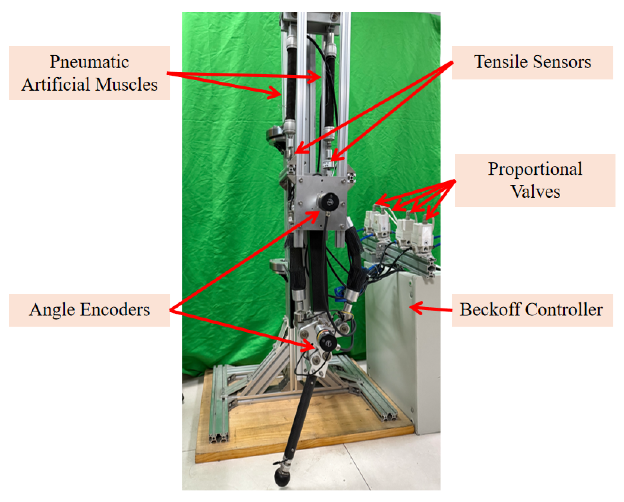
The PAM-driven biomimetic leg joints system design of the robotic joints considers both actuation and structural requirements. Four proportional valves are installed to control the airflow supplied to the muscles. Two angle encoders are mounted to measure the joint motion. Proportional valves are connected to regulate the supply pressure, while a switching power supply is located to provide electrical power for the system. The PAM serves as the system’s primary actuator. Two tension sensors are mounted to measure the muscle force output, and the Beckhoff controller is used as the central control unit to manage system operation as shown in Figure 2.

Structurally, both the hip and knee joints are configured with a single rotational degree of freedom to satisfy the kinematic demands of bipedal locomotion. The hip joint features two symmetrically arranged PAMs of equal initial length with a fixed moment arm of $r_1=0.05\mathrm{m}$. In contrast, the knee joint adopts a crossed four-bar linkage mechanism, which provides a variable instantaneous center of rotation and thereby enhances its kinematic adaptability during gait.

2.2. Kinematic Model

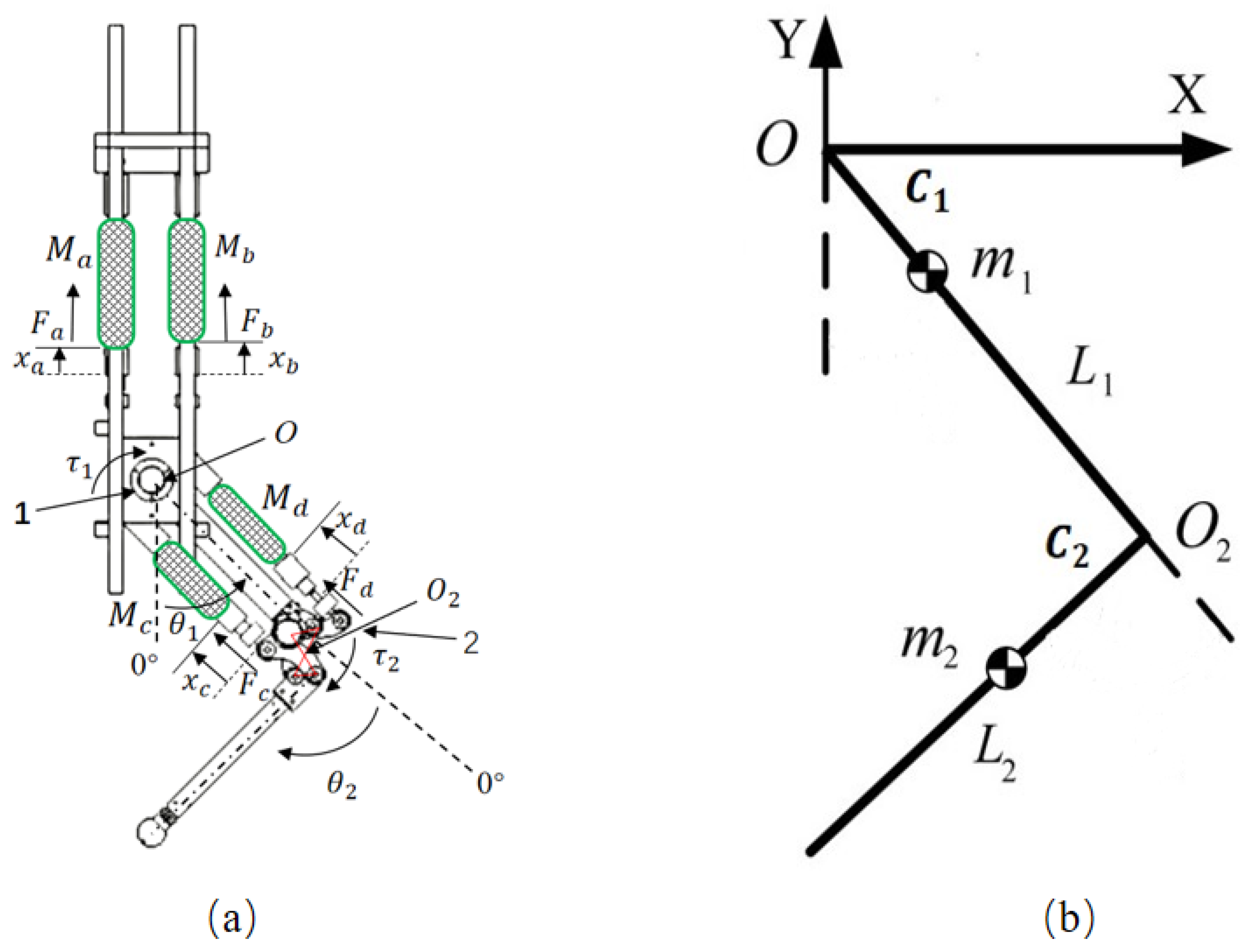
The PAM-driven biomimetic leg joints system consists of a mechanical torso, thigh, and calf. The kinematic model of the PAM-driven leg joints system is illustrated in Figure 3a, where label 1 denotes the hip joint and label 2 denotes the knee joint. The hip joint rotation center is defined as the origin O of a cartesian coordinate system, and point $O_2$ approximates the ICR of the knee joint.

The joint angles ${\theta }_1$ and ${\theta }_2$ represent the hip and knee joint angles, respectively, with the clockwise direction defined as positive. The corresponding joint torques are denoted as ${\tau }_1$ for the hip and ${\tau }_2$ for the knee. Each actuator $M_i$ denotes a PAM. The subscript $i=a, b, c, d$ indexes the four PAMs used in the antagonistic configuration. $x_i$ and $F_i$ represent the muscle’s end displacement and tensile force, respectively.

The position ${\theta }_{h1}=1.22$ rad corresponds to the state where the PAM $M_b$ is fully contracted and the PAM $M_a$ is fully relaxed. Conversely, the position ${\theta }_{h2}=-0.35$ rad corresponds to the state where the PAM $M_b$ is fully relaxed and the PAM $M_a$ is fully contracted. Therefore, the end displacements $x_a$ and $x_b$ of the PAMs $M_a$ and $M_b$ can be expressed in terms of the hip joint angle.

$$x_a=r_1({\theta }_{h1}+{\theta }_1),$$

(1)

$$x_b=r_1({\theta }_{h2}-{\theta }_1).$$

(2)

Assumption 1. 

The four-bar knee mechanism is used to derive the kinematic mapping from ${\theta }_2$ to the PAM end displacements, and the resulting mapping is assumed to be valid within the designed knee motion range.

The four-bar linkage of the knee joint enables a rotational range of up to 1.75 rad. Based on the geometric parameters of the knee-joint linkage and the predefined attachment locations, a kinematic mapping is established to relate the joint rotation to the end displacements of the two PAM actuation paths. Specifically, $x_c$ and $x_d$ can be expressed as functions of ${\theta }_2$ as follows:

$$x_c=a_2{\theta }_2^2+a_1{\theta }_2+a_0,$$

(3)

$$x_d=b_2{\theta }_2^2+b_1{\theta }_2+b_0.$$

(4)

By substituting the knee joint mechanism parameters into the system kinematics model, the results can be obtained separately as $a_2=0.0006466$, $a_1=0.1821$, $a_0=-0.309$, $b_2=0.001009$, $b_1=-0.4291$, $b_0=43.15$. It is worth noting that this polynomial mapping is derived from an analytical geometry–based solution of the four-bar linkage kinematics, and is introduced to provide an explicit closed-form relationship between the joint rotation and the PAM end displacements. According to Equations (3) and (4), the force arm of PAMs tension on the ICR is obtained as follows:

$$l_c=c_3{\theta }_2^3+c_2{\theta }_2^2+c_1{\theta }_2+c_0,$$

(5)

$$l_d=d_3{\theta }_2^3+d_2{\theta }_2^2+d_1{\theta }_2+d_0,$$

(6)

where $c_3=-1.347$, $c_2=1.806$, $c_1=2.509$, $c_0=35.34$, $d_3=0.9856$, $d_2=-6.325$, $d_1=3.844$, $d_0=39.41$, $l_c$ and $l_d$ are the knee joint lever arms by the tensile force $F_c$ and $F_d$.

2.3. Dynamic Model

The PAM-driven biomimetic leg joints system is modeled as a simplified two-degree-of-freedom planar dual-link system, as illustrated in Figure 3b. The thigh and calf segments are represented as rigid links with concentrated masses.

Let $m_1$ and $m_2$ denote the masses of the thigh and calf, respectively. The lengths of the corresponding fixed segments are defined as $L_1$ and $L_2$. The distances from the center of mass of each link to its proximal joint are given by $C_1$ and $C_2$, respectively. The moments of inertia of the thigh and calf about their respective centers of mass are denoted by $I_1$ and $I_2$.

Assumption 2. 

The system is modeled as a planar two-DOF rigid-link mechanism, while out-of-plane motions, structural compliance, and joint backlash are neglected.

The system’s equations of motion can be obtained by using the Lagrangian dynamic modeling approach.

$${\mathit{\tau }}_j={\displaystyle \frac{d}{dt}}({\displaystyle \frac{\partial L}{\partial {\dot{\theta }}_j}})-{\displaystyle \frac{\partial L}{\partial {\theta }_j}},$$

(7)

where j = 1, 2 represents the corresponding joint. L is the Lagrangian function defined as

$$L=T-U,$$

(8)

in which T and U represent the system’s kinetic and potential energy, respectively, as follows:

$$\begin{array}{cc}\hfill T=& {\displaystyle \frac{1}{2}}{({\dot{\theta }}_1+{\dot{\theta }}_2)}^2[m_2{C}_2^2+I_2]+{\displaystyle \frac{1}{2}}{\dot{\theta }}_1[m_1{C}_1^2+m_2{L}_2^2+I_1]+{\dot{\theta }}_1({\dot{\theta }}_1+{\dot{\theta }}_2)m_2{L}_2{I}_{2}cos{\theta }_2,\hfill \end{array}$$

(9)

$$U=-g{m}_1{C}_{1}cos{\theta }_1-g{m}_2[L_{2}cos{\theta }_1+C_{2}cos({\theta }_1+{\theta }_2)].$$

(10)

By substituting (8)–(10) into (7), the dynamic equation of the system can be obtained:

$$\left[\begin{array}{cc}{M}_{11}& M_{12}\\ M_{21}& M_{22}\end{array}\right]\left[\begin{array}{c}{\ddot{\theta }}_1\\ {\ddot{\theta }}_2\end{array}\right]+\left[\begin{array}{c}{H}_{11}\\ H_{21}\end{array}\right]+\left[\begin{array}{c}{G}_{11}\\ G_{21}\end{array}\right]=\left[\begin{array}{c}{\tau }_1\\ {\tau }_2\end{array}\right],$$

(11)

where the submatrices are shown in

Table 1. Model matrix elements.

Submatrix	Component
$M_{11}$	$m_1{C}_1^2+m_2(L_1^2+C_2^2+2L_1{C}_{2}cos{\theta }_2)$$+I_1+I_2$
$M_{12}$	$m_2(C_1^2+L_1{C}_{2}cos{\theta }_2)+I_2$
$M_{21}$	$m_2(C_1^2+L_1{C}_{2}cos{\theta }_2)+I_2$
$M_{22}$	$m_2{C}_2^2+I_2$
$H_{11}$	$m_2{L}_1{C}_{2}sin{\theta }_2{\dot{\theta }}_1{\dot{\theta }}_2-({\dot{\theta }}_1+$${\dot{\theta }}_2)m_2{L}_1{C}_{2}sin{\theta }_2{\dot{\theta }}_2$
$H_{21}$	$m_2{L}_1{C}_{2}sin{\theta }_2{\dot{\theta }}_1^2$
$G_{11}$	$m_{1}g{C}_{1}sin{\theta }_1+m_{2}g{L}_{1}sin{\theta }_1+m_{2}g$$C_{2}cos({\theta }_1+{\theta }_2)$
$G_{12}$	$m_{2}g{C}_{2}sin({\theta }_1+{\theta }_2)$

, the specific physical meanings of the submatrix symbols are shown in

Table 2. Table of variables.

Submatrix	Component
${\theta }_1$	The hip joint rotation angle
${\theta }_2$	The knee joint rotation angle
$m_1$	The weight of the hip joint
$m_2$	The weight of the knee joint
$L_1$	The length of the thigh
$L_2$	The length of the shank
$C_1$	Distance from thigh centroid to hip joint
$C_2$	Distance from calf centroid to knee joint
$I_1$	The moment of inertia of the thigh
$I_2$	The moment of inertia of the calf

.

The driving torque of the hip joint ${\tau }_1$ is related to the antagonistic PAMs tensile force $F_a$ and $F_b$. The PAMs tensile force $F_c$ and $F_d$ drive the knee joint to rotate through a four-bar linkage structure. ${\tau }_2$ is the driving torque of the knee joint, $l_c$ and $l_d$ represent the approximate arm of tensile force. The driving torques of hip and knee joint are as follows:

$$\begin{array}{c}\hfill {\tau }_1=(F_a-F_b)r_1,\end{array}$$

(12)

$$\begin{array}{c}\hfill {\tau }_2=F_c{l}_c-F_d{l}_d.\end{array}$$

(13)

PAMs can only generate unidirectional tensile forces. The mapping relationship between the hip joint torque ${\mathit{\tau }}_1$ and the PAM tensile forces $F_a$ and $F_b$ is designed as follows:

$$F_a=\left\{\begin{array}{c}{\displaystyle \frac{{\tau }_0+{\tau }_1}{r_1}}({\tau }_1\ge 0),\hfill \\ {\displaystyle \frac{{\tau }_0}{r_1}}({\tau }_1<0),\hfill \end{array}\right.$$

(14)

$$F_b=\left\{\begin{array}{c}{\displaystyle \frac{{\tau }_0}{r_1}}({\tau }_1\ge 0),\hfill \\ {\displaystyle \frac{{\tau }_0-{\tau }_1}{r_1}}({\tau }_1<0),\hfill \end{array}\right.$$

(15)

where ${\tau }_0$ is the $F_a$, $F_b$, $F_c$ and $F_d$ applied initial torque. Enforcing ${\tau }_0\ge 0$ ensures that the antagonistic PAM pair remains in tension at all times; otherwise, one muscle may slacken and buckle, which would compromise the accuracy of the mapping from the joint angle to the PAM end displacement.Similarly, the mapping relationship between the hip joint torque ${\tau }_2$ and the PAM tensile forces $F_c$ and $F_d$ is designed as follows:

$$\begin{array}{c}\hfill F_c=\left\{\begin{array}{c}{\displaystyle \frac{{\tau }_0+{\tau }_2}{l_c}}({\tau }_2\ge 0),\hfill \\ {\displaystyle \frac{{\tau }_0}{l_c}}({\tau }_2<0),\hfill \end{array}\right.\end{array}$$

(16)

$$\begin{array}{c}\hfill F_d=\left\{\begin{array}{c}{\displaystyle \frac{{\tau }_0}{l_d}}({\tau }_2\ge 0),\hfill \\ {\displaystyle \frac{{\tau }_0-{\tau }_2}{l_d}}({\tau }_2<0).\hfill \end{array}\right.\end{array}$$

(17)

3. Controller Design

3.1. Constraint Equation

From a universal perspective, the control algorithm design in this section is developed based on a common dynamic equation of a PAM-driven biomimetic leg joints system. Consider a PAM-driven biomimetic leg joints system as follows:

$$\begin{array}{c}\mathbf{M}(\mathit{q}\left(t\right), t)\ddot{\mathit{q}}\left(t\right)+\mathbf{H}(\dot{\mathit{q}}\left(t\right), \mathit{q}\left(t\right), t)+\mathbf{G}(\mathit{q}\left(t\right), t)=\mathit{\tau }\left(t\right),\end{array}$$

(18)

where the generalized coordinate $\mathit{q}$ is an $n\times 1$ vector and n represents the number of degrees of freedom. Equation (11) is the same case of (18) when $n=2$, and $\mathit{q}={[{\theta }_1,{\theta }_2]}^T$, $\dot{\mathit{q}}={[{\dot{\theta }}_1,{\dot{\theta }}_2]}^T$, $\ddot{\mathit{q}}={[{\ddot{\theta }}_1,{\ddot{\theta }}_2]}^T$.

Let the system (18) follow a set of desired trajectories in a trajectory tracking problem. The tracking trajectory ${\theta }_i^d$ of the i-th joint can be formulated as servo constraints:

$$\mathbf{\Lambda }\left(t\right)\mathit{q}\left(t\right)={\mathit{c}}_{\mathbf{0}}\left(t\right),$$

(19)

where $\mathbf{\Lambda }$ is an $n\times n$ identity matrix, ${\mathit{c}}_{\mathbf{0}}\left(t\right)={[{\theta }_1^d\left(t\right),{\theta }_2^d\left(t\right),\dots ,{\theta }_i^d\left(t\right)]}^T$. By differentiating Equation (19) twice with respect to time, the first and second-order matrix forms of the constraint equation can be obtained as:

$$\begin{array}{c}\hfill \mathbf{\Lambda }\left(t\right)\dot{\mathit{q}}\left(t\right)={\mathit{c}}_{\mathbf{1}}\left(t\right),\end{array}$$

(20)

$$\begin{array}{c}\hfill \mathbf{\Lambda }\left(t\right)\ddot{\mathit{q}}\left(t\right)={\mathit{c}}_{\mathbf{2}}\left(t\right),\end{array}$$

(21)

where $c_i$ (i = 0, 1, 2) denotes the i-th order constraint, ${\mathit{c}}_{\mathbf{1}}\left(t\right)={[{\dot{\theta }}_1^d\left(t\right),{\dot{\theta }}_2^d\left(t\right),\dots ,{\dot{\theta }}_n^d\left(t\right)]}^T$, ${\mathit{c}}_{\mathbf{2}}\left(t\right)={[{\ddot{\theta }}_1^d\left(t\right),{\ddot{\theta }}_2^d\left(t\right),\dots ,{\ddot{\theta }}_n^d\left(t\right)]}^T$.

The constraint-following in this paper adheres to second-order servo constraints. The second-order constraint (21) can fully express the constraint information with a given initial condition. Practically all the performance requirements of systems can be formulated as servo constraints. The explicit closed-form constraint can be obtained, which enables control algorithm design. Second-order constraints can help to account for uncertainties and disturbances in the system dynamics. The proposed control algorithm is integrated with the Udwadia controller for constraint-following control, leading to an advanced control structure capable of dealing with time-varying uncertainties simultaneously.

3.2. Adaptive Robust Controller with Uncertainties

In practical situations, uncertainty and interference are inevitable. To account for the uncertainty, the motion Equation (18) is re-described as follows:

$$\mathbf{M}(\mathit{q}\left(t\right), \sigma \left(t\right), t)\ddot{\mathit{q}}\left(t\right)+\mathbf{H}(\mathit{q}\left(t\right), \dot{\mathit{q}}\left(t\right), \sigma \left(t\right), t)+\mathbf{G}(\mathit{q}\left(t\right), \sigma \left(t\right), t)=\mathit{\tau }\left(t\right),$$

(22)

where $\sigma$$\in R^p$ is time-varying uncertain parameters. Based on whether they contain uncertainty or not, the model parameters can be resolved into two parts:

Assumption 3. 

PAM non-idealities are not explicitly modeled, but lumped into the uncertainty term, which is compensated online by the proposed adaptive robust controller.

$$\mathbf{M}(\mathit{q}\left(t\right),\sigma \left(t\right),t)=\overline{\mathit{M}}(\mathit{q}\left(t\right),t)+▵\mathbf{M}(\mathit{q}\left(t\right),\sigma \left(t\right),t),$$

(23)

$$\mathbf{H}(\mathit{q}\left(t\right),\dot{\mathit{q}}\left(t\right),\sigma \left(t\right),t)=\overline{\mathbf{H}}(\mathbf{q},\mathit{q}\left(t\right),t)+\Delta \mathbf{H}(\mathit{q}\left(t\right),\dot{\mathit{q}}\left(t\right),\sigma \left(t\right),t),$$

(24)

$$\mathbf{G}(\mathit{q}\left(t\right),\sigma \left(t\right),t)=\overline{\mathit{G}}(\mathit{q}\left(t\right),t)+▵\mathbf{G}(\mathit{q}\left(t\right),\sigma \left(t\right),t),$$

(25)

where $\overline{\mathit{M}}(·),\overline{\mathit{H}}(·)$, and $\overline{\mathit{G}}(·)$ are the nominal matrices, $▵\mathbf{M}(·)$, $▵\mathbf{H}(·)$, $▵\mathbf{G}(·)$ are the related ambiguity matrices which represents the uncertainty. In an ideal and uncertainty-free system, the uncertainty matrix term is 0.

Design explicit constraint-following term and robust terms based on the Udwadia controller as below:

$${\mathit{p}}_{\mathbf{1}}={\overline{\mathit{M}}}^{\frac{1}{2}}{(\mathbf{\Lambda }{\overline{\mathit{M}}}^{-\frac{1}{2}})}^{+}({\mathit{c}}_{\mathbf{2}}-\mathbf{\Lambda }{\overline{\mathit{M}}}^{-1}\overline{\mathit{Q}}-k\mathbf{\Lambda }\dot{\mathit{q}}),$$

(26)

$${\mathit{p}}_{\mathbf{2}}=-k\overline{\mathit{M}}\mathbf{\Lambda }{(\mathbf{\Lambda }{\mathbf{\Lambda }}^T)}^{-1}{\mathit{p}}^{-1}\mathit{\beta },$$

(27)

where $k\in$ $R^{+}$. An increase in the value of k results in a higher degree of robustness.

However, given the presence of uncertainty and disturbances, it is highly unlikely that all constraint conditions can be fulfilled. Thus, we propose a vector $\mathit{\beta }$ to quantify the level of dissatisfaction with regard to ideal constraints.

$$\begin{array}{cc}\hfill \mathit{\beta }(\mathit{q}\left(t\right),\dot{\mathit{q}}\left(t\right),t)& =\left(\mathbf{\Lambda }(\mathit{q}\left(t\right),\dot{\mathit{q}}\left(t\right),t)\dot{\mathit{q}}\left(t\right)-{\mathit{c}}_1(\mathit{q}\left(t\right),\dot{\mathit{q}}\left(t\right),t)\right)\hfill \\ \hfill & + \lambda \left(\mathbf{\Lambda }(\mathit{q}\left(t\right),\dot{\mathit{q}}\left(t\right),t)\dot{\mathit{q}}\left(t\right)-{\mathit{c}}_0(\mathit{q}\left(t\right),\dot{\mathit{q}}\left(t\right),t)\right),\hfill \end{array}$$

(28)

where $\mathit{\beta }$ takes into account both the first-order and second-order constraints, which can adequately capture the influence of uncertainties and disturbances.

Assumption 4. 

Given $\mathbf{P}\in R^{m\times n}$, $\mathbf{P}>$ 0, let

$$\begin{array}{cc}\hfill \mathbf{W}\left(\mathit{q}\right(t),\sigma (t),t)& =\mathbf{P}\mathbf{\Lambda }(\mathit{q}\left(t\right),t)\overline{\mathit{M}}(\mathit{q}\left(t\right),t)\mathit{M}(\mathit{q}\left(t\right),\sigma \left(t\right),t)\hfill \\ \hfill & \times \overline{\mathit{M}}(\mathit{q}\left(t\right),t){\mathbf{\Lambda }}^T(\mathit{q}\left(t\right),t){\left(\mathbf{\Lambda }(\mathit{q}\left(t\right),t){\mathbf{\Lambda }}^T(\mathit{q}\left(t\right),t)\right)}^{-1}{\mathbf{P}}^{-1}.\hfill \end{array}$$

(29)

A constant ρ_E > −1 can be found, for all ($\mathit{q}$, t) ∈ Rⁿ×R,

$${\displaystyle \frac{1}{2}}min{\lambda }_m\left(\mathbf{W}(\mathit{q}\left(t\right),\sigma \left(t\right),t)\right)\ge {\rho }_E.$$

(30)

Assumption 5. 

(1) There exists a positive constant vector α, and a function $\Pi (·)\in$ Rⁿ × Rⁿ × R, such that

$$\begin{array}{c}{(1+{\rho }_E)}^{-1}max[\parallel \mathit{PA}({\mathit{M}}^{-1}-{\overline{\mathit{M}}}^1)(-\mathit{H}-\mathit{G}+{\mathit{p}}_{\mathbf{1}}+{\mathit{p}}_{\mathbf{2}})\parallel ]\le \mathbf{\Pi }.\hfill \end{array}$$

(31)

(2) Every (α, $\mathit{q}$(t),$\dot{\mathit{q}}$(t),t), the function Π(·) is possible to perform a linear factorization of α: there is a function Π(·): $R^2$ × $R^2$ × R → $R_{+}^k$ such that:

$$\mathbf{\Pi }(\mathit{\alpha },\mathit{q}\left(t\right),\dot{\mathit{q}}\left(t\right),t)={\mathit{\alpha }}^T\tilde{\mathbf{\Pi }}(\mathit{q}\left(t\right),\dot{\mathit{q}}\left(t\right),t),$$

(32)

where α is unknown. The selection of the known function Π is not unique, as long as Assumption 4

By incorporating the above assumption and system dynamics, the following control law is proposed to ensure trajectory tracking under uncertainties

$$\begin{array}{c}\mathit{\tau }\left(t\right)={\mathit{p}}_{\mathbf{1}}(\mathit{q}\left(t\right),\dot{\mathit{q}}\left(\mathit{t}\right),\mathit{t})+{\mathit{p}}_{\mathbf{2}}(\mathit{q}\left(t\right),\dot{\mathit{q}}\left(t\right),t)+{\mathit{p}}_{\mathbf{3}}(\tilde{\mathit{\alpha }},\mathit{q}\left(t\right),\dot{\mathit{q}}\left(t\right),t),\end{array}$$

(33)

where

$$\begin{array}{cc}\hfill {\mathit{p}}_3& =-\left[\overline{\mathit{M}}(\mathit{q}\left(t\right),t){\mathbf{\Lambda }}^T(\mathit{q}\left(t\right),t){\left(\mathbf{\Lambda }(\mathit{q}\left(t\right),t){\mathbf{\Lambda }}^T(\mathit{q}\left(t\right),t)\right)}^{-1}{\mathbf{P}}^{-1}\right]\mathit{\gamma }(\tilde{\mathit{\alpha }},\mathit{q}\left(t\right),\dot{\mathit{q}}\left(t\right),t)\hfill \\ \hfill & + \mathit{\mu }(\tilde{\mathit{\alpha }},\mathit{q}\left(t\right),\dot{\mathit{q}}\left(t\right),t)\mathbf{\Pi }(\tilde{\mathit{\alpha }},\mathit{q}\left(t\right),\dot{\mathit{q}}\left(t\right),t),\hfill \end{array}$$

(34)

$$\mathit{\gamma }(\tilde{\mathit{\alpha }},\mathit{q}\left(t\right),\dot{\mathit{q}}\left(t\right),t)=\left\{\begin{array}{c}{\displaystyle \frac{1}{\epsilon }}, \mathrm{if}\parallel \mu (\tilde{\mathit{\alpha }},\mathit{q}\left(t\right),\dot{\mathit{q}}\left(t\right),t)\parallel \le \widehat{\epsilon },\hfill \\ {\displaystyle \frac{1}{\parallel \mu (\tilde{\mathit{\alpha }},\mathit{q}\left(t\right),\dot{\mathit{q}}\left(t\right),t)\parallel }},\mathrm{if}\mathrm{else}\end{array}\right.$$

(35)

$$\begin{array}{c}\mathit{\mu }(\tilde{\mathit{\alpha }},\mathit{q}\left(t\right),\dot{\mathit{q}}\left(t\right),t)=\mathit{\beta }\mathbf{\Pi }(\mathit{\alpha },\mathit{q}\left(t\right),\dot{\mathit{q}}\left(t\right),t).\end{array}$$

(36)

The parameter $\tilde{\mathit{\alpha }}$ is governed by the following adaptive law

$$\dot{\tilde{\mathit{\alpha }}}={\displaystyle \frac{\Gamma }{1+{\parallel \tilde{\mathbf{\Pi }}(q\left(t\right),\dot{q}\left(t\right),t)\parallel }^2}}\tilde{\mathbf{\Pi }}(q\left(t\right),\dot{q}\left(t\right),t)\parallel \mathit{\beta }\parallel -k_2\tilde{\mathit{\alpha }}.$$

(37)

The initial conditions are selected to be positive, which ensures that $\tilde{\mathit{\alpha }}$ are positive for all t. By introducing a normalization factor ${\displaystyle \frac{\Gamma }{1+{\parallel \tilde{\mathbf{\Pi }}(q\left(t\right),\dot{q}\left(t\right),t)\parallel }^2}}$, the adaptation step is automatically limited, preventing parameter blow-up and unfavorable transients. As a result, the control algorithm avoids aggressive torque commands near saturation, mitigating chatter and prolonging hardware lifetime. In addition, reduced high-frequency compensation lowers compressed-air usage and peak power, yielding smoother valve actuation and decreased pneumatic consumption.

3.3. Stability Analysis

Theorem 1. 

Let $\tilde{\mathit{\delta }}:={\left[{\mathit{\beta }}^T{(\tilde{\mathit{\alpha }}-\mathit{\alpha })}^T\right]}^T\in {\mathit{R}}^{m+k}$. Subject to Assumptions 4 and 5, consider the system (22). The control (33) renders the following performance:

(i) UB: For any $r>0$, there is a $d\left(r\right)<\infty$ such that if $\parallel \tilde{\mathit{\delta }}\left(t_0\right)\parallel \le r$, then $\parallel \tilde{\mathit{\delta }}\left(t\right)\parallel \le d\left(r\right)$ for all $t\ge t_0$.

(ii) UUB: For any $r>0$ with $\parallel \tilde{\mathit{\delta }}\left(t_0\right)\parallel \le r$, there exists a $\overline{d}>0$ such that $\parallel \tilde{\mathit{\delta }}\parallel \le \overline{d}$ for any $\overline{d}\ge d$ as $t\ge t_0+T(\overline{d},r)$, where $T(\overline{d},r)<\infty$.

Let $▵\mathbf{D}($$\mathbf{q}$$,\sigma ,t)$ := ${\mathbf{M}}^{-1}$$(\mathbf{q},\sigma ,t)$ − ${\overline{\mathbf{M}}}^{-1}$$(\mathbf{q},t)$. Then,

$$\mathbf{E}(\mathbf{q},\sigma ,t)=\overline{\mathbf{M}}(\mathbf{q},t)({\mathbf{M}}^{-1}(\mathbf{q},\sigma ,t)-{\overline{\mathbf{M}}}^{-1}(\mathbf{q},t)),$$

(38)

$$▵\mathbf{D}(\mathbf{q},\sigma ,t)=\mathbf{D}(\mathbf{q},t)\mathbf{E}(\mathbf{q},\sigma ,t),$$

(39)

$${\mathbf{M}}^{-1}(\mathbf{q},\sigma ,t)=▵\mathbf{D}(\mathbf{q},\sigma ,t)+\mathbf{D}(\mathbf{q},t).$$

(40)

Proof. 

A legitimate Lyapunov function candidate is given:

$$V(\mathit{\beta },\tilde{\mathit{\alpha }})={\mathit{\beta }}^T\mathbf{P}\mathit{\beta }+{\Gamma }^{-1}(1+{\rho }_E){(\tilde{\mathit{\alpha }}-\mathit{\alpha })}^T(\tilde{\mathit{\alpha }}-\mathit{\alpha }).$$

(41)

For given controlled system with uncertainty and desired trajectory, the derivative of V is evaluated as follows:

$$\dot{\mathit{V}}=2{\mathit{\beta }}^T\mathbf{P}\dot{\mathit{\beta }}+2{\Gamma }^{-1}(1+{\rho }_E){(\tilde{\mathit{\alpha }}-\mathit{\alpha })}^T\dot{\tilde{\mathit{\alpha }}}.$$

(42)

The first term of (41) can be evaluated as follows:

$$\begin{array}{cc}\hfill 2{\mathit{\beta }}^T\mathbf{P}\dot{\mathit{\beta }}& =2{\mathit{\beta }}^T\mathbf{P}\left[\mathbf{\Lambda }\ddot{\mathit{q}}-{\mathit{c}}_2+\lambda (\mathbf{\Lambda }\dot{\mathit{q}}-{\mathit{c}}_1)\right]\hfill \\ \hfill & =\left[\mathbf{\Lambda }\mathbf{D}(-\overline{\mathit{H}}-\overline{\mathit{G}})+\mathbf{\Lambda }\mathbf{D}{\mathit{p}}_1-{\mathit{c}}_2+\lambda (\mathbf{\Lambda }\dot{\mathit{q}}-{\mathit{c}}_1)\right]+\mathbf{\Lambda }\mathbf{D}{\mathit{p}}_2\hfill \\ \hfill & +\mathbf{\Lambda }(▵\mathbf{D}+\mathbf{D}){\mathit{p}}_3+[\mathbf{\Lambda }\mathbf{D}(-▵\mathit{H}-▵\mathit{G})+\mathbf{\Lambda }▵\mathbf{D}(-\mathit{H}-\mathit{G})\hfill \\ \hfill & +\mathbf{\Lambda }▵\mathbf{D}({\mathit{p}}_1+{\mathit{p}}_2)].\hfill \end{array}$$

(43)

With the special case $\sigma$ = 0, (26) can be written as

$$\mathbf{\Lambda }\mathit{D}(-\overline{\mathit{H}}-\overline{\mathit{G}})+\mathbf{\Lambda }\mathit{D}{\mathit{p}}_{\mathbf{1}}-{\mathit{c}}_{\mathbf{2}}+\lambda (\mathbf{\Lambda }\dot{\mathit{q}}-{\mathit{c}}_{\mathbf{1}})=0,$$

(44)

From the above formula that (43) can be evaluated as

$$\begin{array}{l}2{\mathit{\beta }}^T\mathbf{P}[\mathbf{\Lambda }\mathit{D}(-▵\mathit{H}-▵\mathit{G})+\mathbf{\Lambda }▵\mathit{D}(-\mathit{H}-\mathit{G})+\mathbf{\Lambda }▵\mathit{D}({\mathit{p}}_{\mathbf{1}}+{\mathit{p}}_{\mathbf{2}})]\\ \le 2\parallel \mathit{\beta }\parallel \parallel \mathbf{P}[\mathbf{\Lambda }\mathit{D}(-▵\mathit{H}-▵\mathit{G})+\mathbf{\Lambda }▵\mathit{D}(-\mathit{H}-\mathit{G})+\mathbf{\Lambda }▵\mathit{D}({\mathit{p}}_{\mathbf{1}}+{\mathit{p}}_{\mathbf{2}})]\parallel \\ \le 2(1+{\rho }_E)\parallel \mathit{\beta }\parallel \Pi (\mathit{\alpha },\mathit{q},\dot{\mathit{q}},t).\end{array}$$

(45)

By (27), we have

$$2{\mathit{\beta }}^T\mathbf{P}\mathbf{\Lambda }\mathit{D}{\mathit{p}}_{\mathbf{2}}=-2k{\mathit{\beta }}^T\mathit{\beta }=-2k{\parallel \mathit{\beta }\parallel }^2.$$

(46)

By (33), (46), (41), we have

$$\begin{array}{c}2{\mathit{\beta }}^T\mathbf{P}\mathbf{\Lambda }(\mathit{D}+▵\mathit{D}){\mathit{p}}_{\mathbf{3}}=2{\mathit{\beta }}^T\mathbf{P}\mathbf{\Lambda }\mathit{D}\mathit{E}[-\overline{M}{\mathbf{\Lambda }}^T{(\mathbf{\Lambda }{\mathbf{\Lambda }}^T)}^{-1}{P}^{-1}\gamma \mathit{\mu }\Pi ]-{2\gamma \parallel \mathit{\beta }\parallel }^2\parallel \mathit{\mu }\parallel .\hfill \end{array}$$

(47)

Based on Assumption 4 and Rayleigh’s principle, we can show that

$$\begin{array}{c}2{\mathit{\beta }}^T\mathbf{P}\mathbf{\Lambda }\mathit{D}\mathit{E}[-\overline{\mathit{M}}{\mathbf{\Lambda }}^T{(\mathbf{\Lambda }{\mathbf{\Lambda }}^T)}^{-1}{\mathbf{P}}^{-1}\gamma \mathit{\mu }\Pi ]\hfill \\ =-2\gamma {\mathit{\mu }}^T\left[\overline{\mathit{M}}{\mathbf{\Lambda }}^T{(\mathbf{\Lambda }{\mathbf{\Lambda }}^T)}^{-1}{\mathbf{P}}^{-1}\right]\mathit{\mu }\hfill \\ =-2\gamma {\mathit{\mu }}^T{\displaystyle \frac{1}{2}}[\overline{\mathit{M}}{\mathbf{\Lambda }}^T{(\mathbf{\Lambda }{\mathbf{\Lambda }}^T)}^{-1}{\mathbf{P}}^{-1}+\overline{\mathit{M}}{\mathbf{\Lambda }}^T{(\mathbf{\Lambda }{\mathbf{\Lambda }}^T)}^{-1}{\mathbf{P}}^{-1}]\hfill \\ =-2\gamma {\mathit{\mu }}^T{\displaystyle \frac{1}{2}}(\mathit{W}+{\mathit{W}}^T)\mathit{\mu }\hfill \\ \le -2\gamma {\rho }_E\parallel \mathit{\mu }\parallel .\hfill \end{array}$$

(48)

Using (47) and (48), we obtain

$$2{\mathit{\beta }}^T\mathbf{P}\mathbf{\Lambda }(\mathit{D}+▵\mathit{D}){\mathit{p}}_{\mathbf{3}}\le -2\gamma (1+{\rho }_E)\parallel \mathit{\mu }\parallel .$$

(49)

(i) If $\parallel \mathit{\mu }\parallel >\widehat{\epsilon }$

$$\begin{array}{c}-2\gamma (1+{\rho }_E)\parallel \mathit{\mu }\parallel =-2\gamma (1+{\rho }_E){\displaystyle \frac{1}{\mathit{\mu }}}{\parallel \mathit{\mu }\parallel }^2=-2\gamma (1+{\rho }_E)\parallel \mathit{\mu }\parallel .\hfill \end{array}$$

(50)

(ii) If $\parallel \mathit{\mu }\parallel \le \widehat{\epsilon }$

$$-2\gamma (1+{\rho }_E)\parallel \mathit{\mu }\parallel =-2\gamma (1+{\rho }_E){\displaystyle \frac{1}{\widehat{\epsilon }}}{\parallel \mathit{\mu }\parallel }^2.$$

(51)

These lead to the following: for $\parallel \mathit{\mu }\parallel >\widehat{\epsilon }$, we have

$$2{\mathit{\beta }}^{T}P\dot{\mathit{\beta }}\le -2\kappa {\parallel \mathit{\beta }\parallel }^2+\left(1+{\rho }_E\right)\left\{-2\parallel \mathit{\beta }\parallel \mathbf{\Pi }(\tilde{\mathit{\alpha }},q,\dot{q},t)+2\parallel \mathit{\beta }\parallel \mathbf{\Pi }(\mathit{\alpha },q,\dot{q},t)\right\}.$$

(52)

For $\parallel \mathit{\mu }\parallel \le \widehat{\epsilon }$

$$\begin{array}{cc}\hfill 2{\mathit{\beta }}^{T}P\dot{\mathit{\beta }}\le & -{2\kappa \parallel \mathit{\beta }\parallel }^2+\left(1+{\rho }_E\right){\displaystyle \frac{\widehat{\epsilon }}{2}}\hfill \\ \hfill & +\left(1+{\rho }_E\right)\left\{-2\parallel \mathit{\beta }\parallel \mathbf{\Pi }(\tilde{\mathit{\alpha }},q,\dot{q},t)+2\parallel \mathit{\beta }\parallel \mathbf{\Pi }(\mathit{\alpha },q,\dot{q},t)\right\}.\hfill \end{array}$$

(53)

Based on Assumption 5, we obtain

$$2\parallel \mathit{\beta }\parallel \mathbf{\Pi }(\mathit{\alpha },\mathit{q},\dot{\mathit{q}},t)-2\parallel \mathit{\beta }\parallel \mathbf{\Pi }(\widehat{\mathit{\alpha }},\mathit{q},\dot{\mathit{q}},t)=2\parallel \mathit{\beta }\parallel {(a-\widehat{\mathit{\alpha }})}^T\tilde{\mathbf{\Pi }}(\mathit{q},\dot{\mathit{q}},t).$$

(54)

For all $\parallel \mathit{\mu }\parallel$, the following inequality holds:

$$\begin{array}{c}2{\mathit{\beta }}^T\mathbf{P}\dot{\mathit{\beta }}\le -{2k\parallel \mathit{\beta }\parallel }^2+(1+{\rho }_E){\displaystyle \frac{\widehat{\epsilon }}{2}}+2(1+{\rho }_E)\parallel \mathit{\beta }\parallel {(a-\widehat{\mathit{\alpha }})}^T\tilde{\mathbf{\Pi }}(\mathit{q},\dot{\mathit{q}},t).\hfill \end{array}$$

(55)

By using adaptive law (37), we have

$$\begin{array}{c}2{\Gamma }^{-1}(1+{\rho }_E){(\tilde{\mathit{\alpha }}-\mathit{\alpha })}^T\dot{\tilde{a}}\hfill \\ \le 2(\tilde{\mathit{\alpha }}-\mathit{\alpha }{)}^T\tilde{\mathbf{\Pi }}(q,\dot{q},t)\parallel \mathit{\beta }\parallel -2{\mathrm{\Gamma }}^{-1}{k}_2\parallel \tilde{\mathit{\alpha }}-\mathit{\alpha }{\parallel }^2+2{\mathrm{\Gamma }}^{-1}{k}_2\parallel \tilde{\mathit{\alpha }}-\mathit{\alpha }\parallel \parallel \mathit{\alpha }\parallel .\end{array}$$

(56)

Combining (19), (20), and (42), we derive

$$\begin{array}{cc}\hfill \dot{V}\le & -{2\kappa \parallel \mathit{\beta }\parallel }^2+(1+{\rho }_E){\displaystyle \frac{\widehat{\epsilon }}{2}}-2{\Gamma }^{-1}{k}_2(1+{\rho }_E){\parallel \tilde{\mathit{\alpha }}-\mathit{\alpha }\parallel }^2\hfill \\ \hfill & +2{\Gamma }^{-1}{k}_2(1+{\rho }_E)\parallel \tilde{\mathit{\alpha }}-\mathit{\alpha }\parallel \parallel \mathit{\alpha }\parallel \hfill \\ \hfill \le & -k_1\parallel \tilde{\mathit{\delta }}{\parallel }^2+k_2\parallel \tilde{\mathit{\delta }}\parallel +k_3,\hfill \end{array}$$

(57)

where

$${\Gamma }^{-1}=min\{2\kappa ,2{\Gamma }^{-1}{k}_2(1+{\rho }_E)\},k_2=2{\Gamma }^{-1}{k}_2(1+{\rho }_E)\parallel \mathit{\alpha }\parallel ,k_3={\displaystyle \frac{(1+{\rho }_E)\widehat{\epsilon }}{2}}.$$

Upon invoking the standard arguments as in Khalil [31] and Chen [32], we conclude the UB with

$$d\left(r\right)=\left\{\begin{array}{cc}\sqrt{{\displaystyle \frac{{\gamma }_2}{{\gamma }_1}}}R,\hfill & r\le R,\hfill \\ \sqrt{{\displaystyle \frac{{\gamma }_2}{{\gamma }_1}}}r,\hfill & r>R,\hfill \end{array}\right.$$

(58)

where

$$R={\displaystyle \frac{1}{2k_1}}\left(k_2+\sqrt{{k_2}^2+4k_1{k}_3}\right),$$

(59)

and ${\gamma }_1=min\{{\lambda }_{min}\left(P\right),{\Gamma }^{-1}(1+{\rho }_E)\}$, ${\gamma }_2=max\{{\lambda }_{max}\left(P\right),{\Gamma }^{-1}(1+{\rho }_E)\}$.

Furthermore, UUB also follows with

$$d=\sqrt{{\displaystyle \frac{{\gamma }_2}{{\gamma }_1}}}R,$$

(60)

$$T(\overline{d},r)=\left\{\begin{array}{cc}0,\hfill & r\le \overline{d}\sqrt{{\displaystyle \frac{{\gamma }_1}{{\gamma }_2}}},\hfill \\ {\displaystyle \frac{{\gamma }_2{r}^2-({\gamma }_1/{\gamma }_2){\overline{d}}^2}{k_1{\overline{d}}^2{({\gamma }_1/{\gamma }_2)}^{1/2}-k_2\overline{d}{({\gamma }_1/{\gamma }_2)}^{1/2}-k_3}},\hfill & \mathrm{otherwise}.\hfill \end{array}\right.$$

(61)

Since the Lyapunov derivative is negative outside a region of $\tilde{\mathit{\delta }}$, one concludes UB and UUB. □

4. Simulation

This section evaluates the performance of the proposed control algorithm described in Section 3 through numerical simulation. The joint control torques are computed based on the control law defined in (33). The parameters used for the model, including physical and control-related constants, are listed in

Table 3. Table with parameters.

Parameters Name	Value
m1	2.97 kg
m2	0.54 kg
I1	0.1175 kg·m2
I2	0.00708 kg·m2
L1	0.4 m
L2	0.355 m
C1	0. 124 m
C2	0.146 m
g	9.8 m/s2

.

We introduced small sinusoidal perturbations to the mass parameters in simulation to emulate typical time-varying parametric uncertainties in a simple, controlled, and repeatable manner. This sinusoidal model is used only as a representative example for robustness evaluation. $m_1\left(t\right)=\overline{m_1}\left(t\right)+▵$$m_1\left(t\right)$, $m_2\left(t\right)=\overline{m_2}\left(t\right)+▵$$m_2\left(t\right)$, $▵m_1\left(t\right)=0.1sin(2$$\pi$$t)$, $▵m_2\left(t\right)=0.1sin(2$$\pi$$t)$. The initial conditions are set as: ${\theta }_1\left(0\right)=0.0872$ rad, ${\theta }_2\left(0\right)$ = 0.4361 rad, $\dot{{\theta }_1}\left(0\right)=0.0017$ rad/s, $\dot{{\theta }_2}\left(0\right)=0.0017$ rad/s. The desired trajectories of joints are set as below:

$$\begin{array}{cc}\hfill & {\theta }_1^d\left(t\right)=(0.4361sin(4/3\pi \ast t)+0.0017),\hfill \end{array}$$

(62)

$$\begin{array}{cc}\hfill & {\theta }_2^d\left(t\right)=(0.6106sin(4/3\pi \ast t)+10sin(8/3\pi \ast t-\pi /4)+0.4361).\hfill \end{array}$$

(63)

The terms in $\mathbf{M}$ are either linear constants of position or linear constants of velocity. Consequently, Assumption 5 can be satisfied by

$$\begin{array}{c}\mathbf{\Pi }(\mathit{\alpha },\mathit{q},\dot{\mathit{q}},t)={\alpha }_1\parallel \dot{\mathit{q}}\parallel + {\alpha }_2\parallel \mathit{q}\parallel +{\alpha }_3\hfill \\ \le \mathit{\alpha }(\parallel \dot{\mathit{q}}\parallel +\parallel \mathit{q}\parallel +1)\hfill \\ =:\mathit{\alpha }\mathbf{\Pi }(\mathit{q},\dot{\mathit{q}},t),\hfill \end{array}$$

(64)

where ${\alpha }_{1,2,3}>0$, ${\alpha }_{1,2,3}$ are representing the first, second, and third components of vector $\mathit{\alpha }$, respectively. $\mathit{\alpha }$ = max [${\alpha }_1,{\alpha }_2,{\alpha }_3$].

The control algorithm parameters for simulation are chosen as follows: k = 10, $\Gamma$ = 50, $\lambda$ = 10, $\epsilon$ = 0.1, $k_2=0.001$, P = $\left[\begin{array}{cc}1& 0\\ 0& 1\end{array}\right]$. Set the system simulation time t = 20 s. In practice, $\Gamma$ is set to achieve a moderate adaptation rate without amplifying noise, $k_2$ is chosen as the smallest value that still guarantees robustness against the lumped uncertainty while avoiding excessive control effort/chattering, $\epsilon$ is selected according to sensor noise/resolution as a small positive regularization constant for numerical stability.

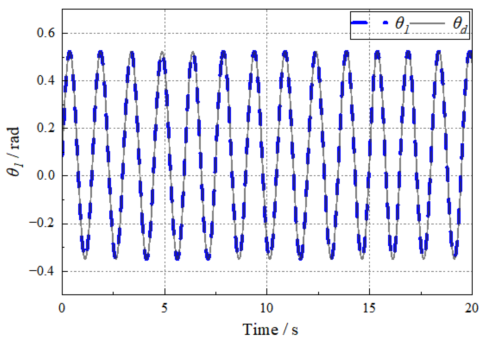
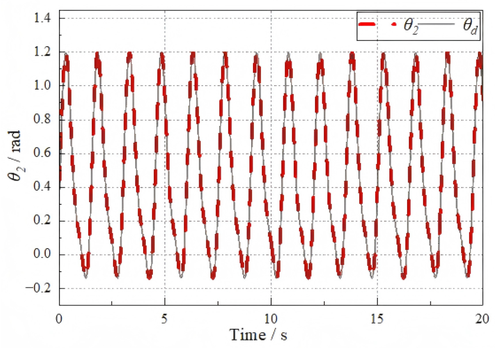
Under the proposed control algorithm, Figure 4 presents the desired and actual trajectories of the hip joint, while Figure 5 shows the corresponding results for the knee joint. In both cases, the actual trajectories closely follow the desired trajectories, indicating satisfactory tracking performance and effective control response.

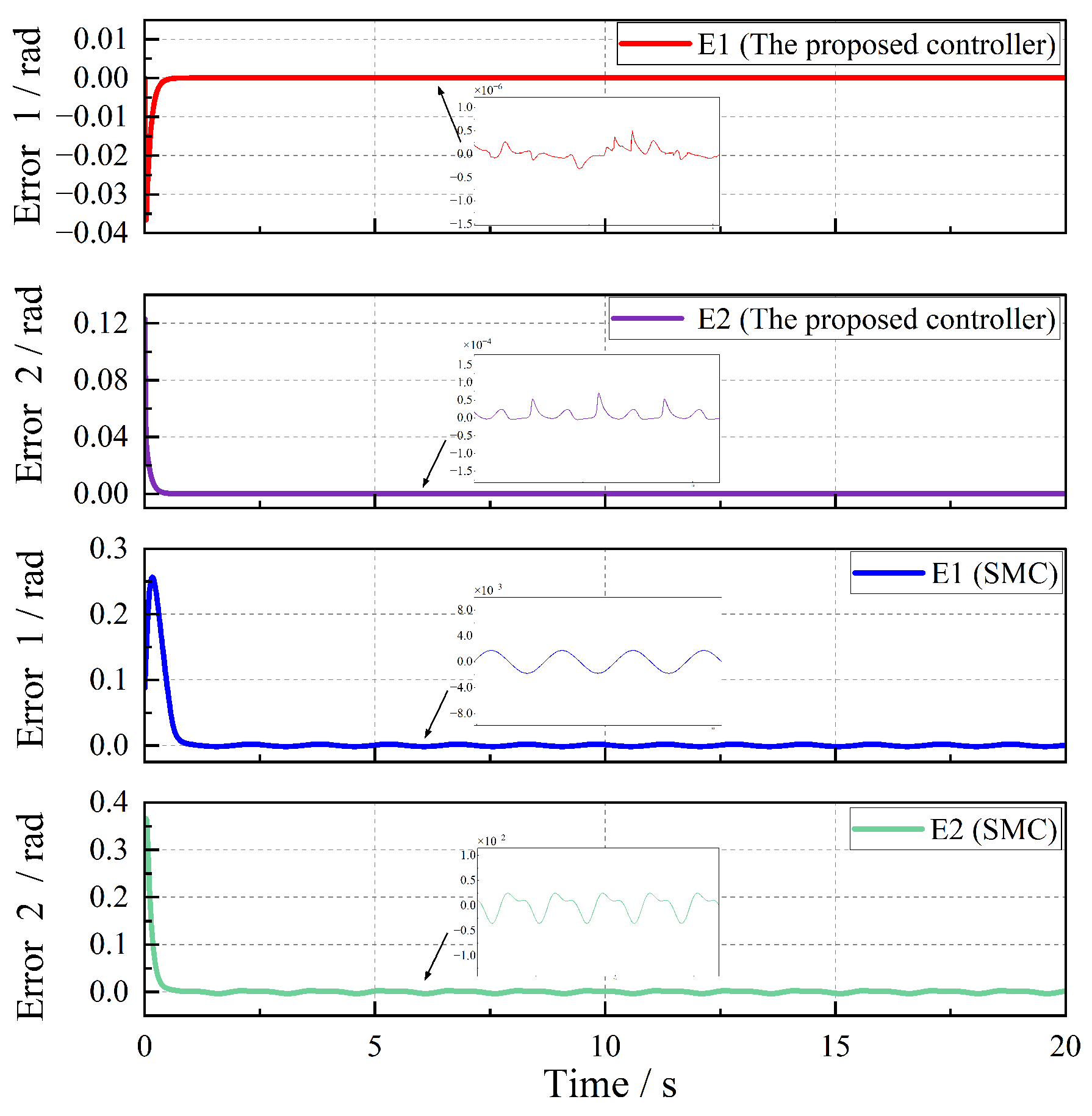
Figure 6 comprises four subplots: the top two illustrate the tracking errors $E_1$ and $E_2$ under SMC, while the bottom two present the same error metrics under adaptive robust control algorithm. Under SMC, both error curves exhibit large initial deviations at $t=0$ s, but rapidly converge to near zero within approximately one second and remain stable thereafter, demonstrating SMC’s strong capability in rejecting parameter uncertainties and external disturbances.

In contrast, adaptive robust control algorithm achieves near-zero tracking errors at the initial moment, indicating superior transient response and ideal tracking performance. Quantitatively, the maximum errors under the adaptive robust control algorithm are only 0.036613 for $E_1$ and 0.1234 for $E_2$, both of which are notably smaller than those observed under SMC. These results confirm that the adaptive robust control algorithm provides reduced maximum and steady-state errors compared to SMC, highlighting its improved tracking precision and robustness.

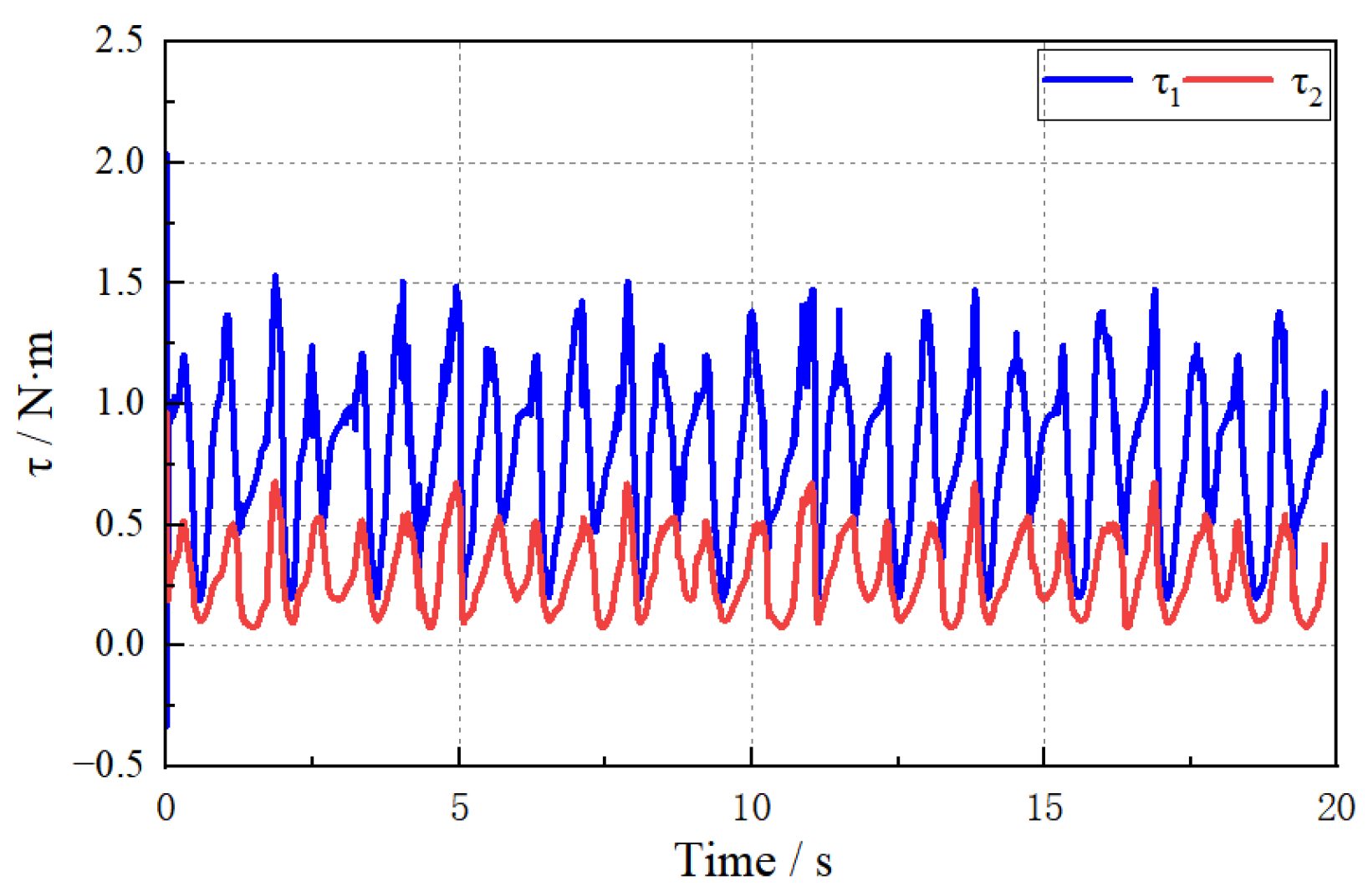
The time-domain responses of the joint torque signals ${\tau }_1$ and ${\tau }_2$ over a 20 s interval are depicted in Figure 7. The torque ${\tau }_1$ exhibits a significantly larger amplitude, peaking at approximately 1.5 $\mathrm{N}·\mathrm{m}$, while ${\tau }_2$ reaches only around 0.4–0.5 $\mathrm{N}·\mathrm{m}$. This disparity suggests that the hip joint experiences a higher inertial load or resistance, thereby requiring greater torque to track the same desired trajectory.

Both torque signals exhibit the same oscillation period, indicating that they are governed by a common desired frequency. A slight phase offset between ${\tau }_1$ and ${\tau }_2$ is evident at their peak values, likely due to inter-joint coupling effects and differing dynamic characteristics between the hip and knee joints. In summary, the larger magnitude of ${\tau }_1$ reflects the increased actuation demand at the hip joint, the smaller amplitude of ${\tau }_2$ corresponds to the relatively load or inertia at the knee joint.

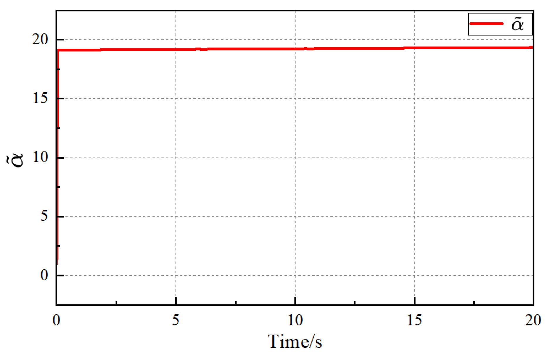
Figure 8 illustrates the time evolution of the adaptive gain $\tilde{a}$ over the 0–20 s simulation interval. At the onset, $\tilde{a}$ rapidly increases from its initial value to approximately 18, followed by a slow and steady rise toward 19 as time progresses. After the initial transient phase, the gain trajectory flattens, indicating that the adaptive law has effectively converged and the control algorithm is making only minor adjustments thereafter. This behavior suggests that the online parameter estimation mechanism rapidly identifies a near-optimal gain and subsequently maintains it with minimal variation, ensuring stable and consistent control performance throughout the simulation.

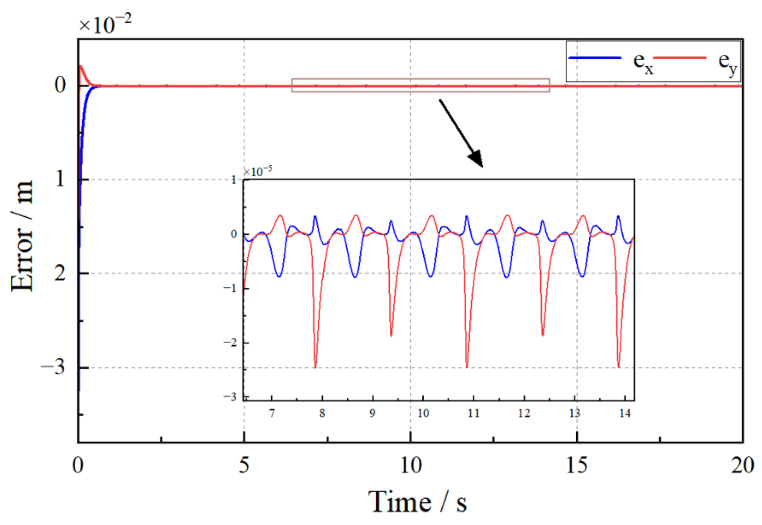
Figure 9 presents the end-effector trajectory error in both the x- and y-directions over a 0–20 s interval, with the vertical axis indicating the position error in meters. At $t=0$ s, both error curves start near $-0.04$ m and exhibit rapid convergence, reaching near-zero values within approximately 0.5 s. For $t>1$ s, the errors remain confined within an extremely narrow oscillatory band around zero, indicating highly precise trajectory tracking.

As shown in the inset, the steady-state fluctuations are on the order of $\pm {10}^{-5}$ m, demonstrating that the proposed control algorithm ensures ultra-high positioning accuracy and robustness throughout prolonged operation. These results confirm the effectiveness of the control scheme in maintaining fine end-point regulation under dynamic conditions.

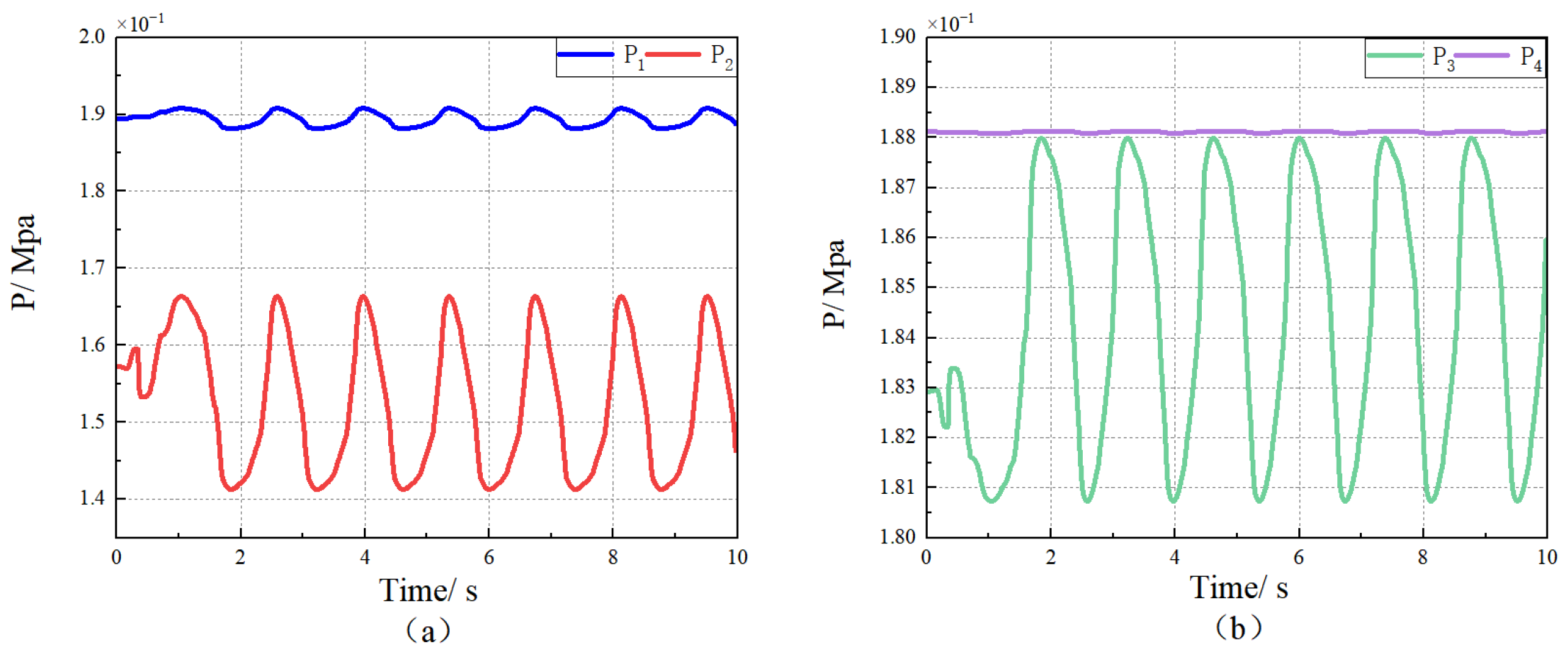
Figure 10 illustrates the air pressures of PAMs. Each joint is controlled by a set of antagonistic PAMs, with one side maintaining a relatively constant air pressure, while the other side undergoes periodic adjustments over time. As shown in Figure 10a is the hip joint, one muscle maintains an approximate constant pressure of about 0.19 MPa, while the opposing muscle exhibits significant periodic fluctuations between approximately 0.14 and 0.17 MPa, achieving a cyclical flexion-extension motion. Similarly, at the knee joint shown in Figure 10b, one muscle maintains a stable pressure of about 0.187 MPa, while the other oscillates periodically within the range of 0.181–0.188 MPa. This pattern reflects a biological antagonistic mechanism, where one muscle provides stable support and the other generates the dynamic changes needed for movement. This coordination ensures the stability of the joint while producing the rhythmic movements required for gait.

Table 4. Tracking error of the hip joint under four algorithms.

Metric	The Proposed Controller	SMC	GA–PID	Torque Compensation Control
Stabilization time (s)	0.0350	0.5700	0.5900	0.0400
MAX (rad)	0.0363	0.2553	0.0889	0.0590
MAE (rad)	0.0007	0.0062	0.0339	0.0104
RMSR (rad)	0.0045	0.0311	0.0377	0.0142
MAPE (%)	0.0661	0.6212	3.3937	1.0449
MRD (%)	0.0661	0.5140	3.3937	0.0344
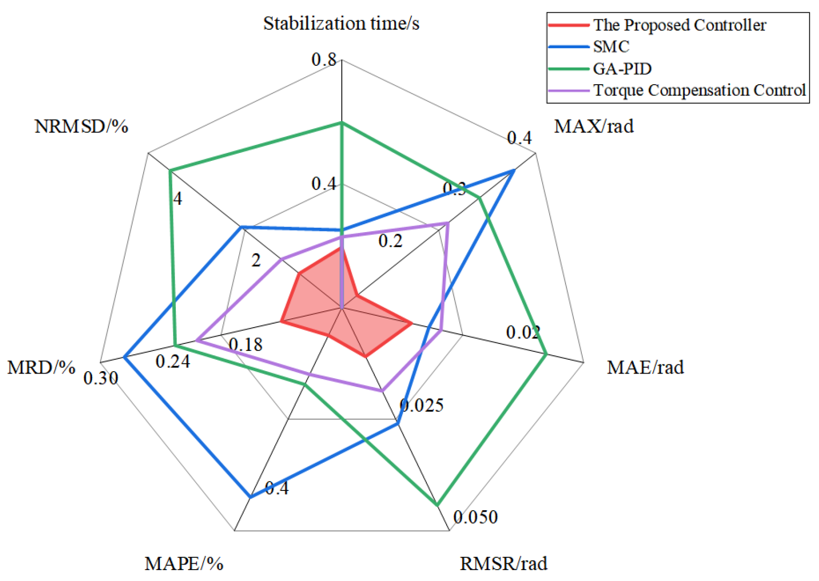
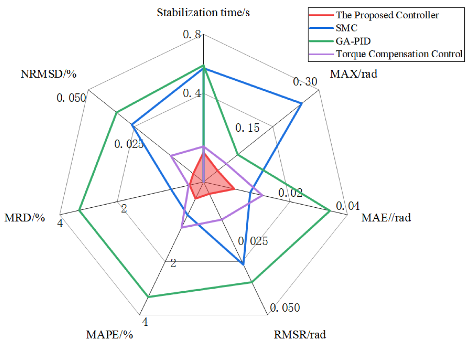
NRMSD (%)	0.0045	0.0311	0.0377	0.0142

and

Table 5. Tracking error of the knee joint under four algorithms.

Metric	The Proposed Controller	SMC	GA–PID	Torque Compensation Control
Stabilization time (s)	0.1940	0.2500	0.5970	0.2280
MAX (rad)	0.1234	0.3663	0.3129	0.2640
MAE (rad)	0.0015	0.0044	0.0238	0.0064
RMSR (rad)	0.0110	0.0260	0.0443	0.0187
MAPE (%)	0.1500	0.4400	0.2380	0.2200
MRD (%)	0.1500	0.2800	0.2380	0.2200
NRMSD (%)	1.1000	2.6000	4.4300	1.5600

respectively summarize the tracking errors of the first and second joint under four control algorithms. The errors include Maximum error (MAX), Mean Absolute Error (MAE), Root Mean Square Residual (RMSR), Mean Absolute Percentage Error (MAPE), Mean Relative Deviation (MRD), Normalized Root Mean Square Deviation (NRMSD). The proposed control algorithm, SMC, GA-PID, and the torque compensation control [33]. To facilitate a more intuitive comparison of each algorithm’s identification and tracking capabilities, the computed performance indicators are visualized in radar chart form in Figure 11 and Figure 12.

To ensure a fair comparison, The SMC parameters are selected as follows: the sliding-surface coefficients are set to $\tilde{\lambda }=[1,1]$, and the reaching-law gains are chosen as $\mathbf{k}=[10,10]$. The PID baseline is tuned using a genetic algorithm. The search ranges of the PID gains are set to $K_p\in [{10}^{-3},20]$, $K_i\in [{10}^{-3},1]$, and $K_d\in [{10}^{-3},1]$. The fitness function is constructed as a weighted combination of tracking error, overshoot, rise time, and settling time, with the corresponding weights selected as $w_e=0.5$, $w_o=0.4$, $w_r=0.9$, and $w_s=0.4$, respectively. For fitness evaluation, the nonlinear plant is linearized at the equilibrium point, yielding $G\left(s\right)=\mathrm{tf}(400,[1,5,0\left]\right)$. The GA uses a population size of 50 and runs for 10 iterations, with a crossover probability of $0.8$, a mutation probability of $0.1$, and a replication probability of $0.2$; the gene length is set to 10. The optimized $(K_p,K_i,K_d)$ obtained by GA is then used for the GA-PID controller in all comparative tests.

In the Figure 11 and Figure 12, the proposed control algorithm exhibits the lowest mean absolute error and root-mean-square error among all control algorithms. This indicates that adaptive robust control algorithm achieves the highest tracking accuracy for both joints, maintaining smooth convergence without overshoot. Compared with SMC, adaptive robust control algorithm reduces high-frequency chattering significantly while preserving robustness to dynamic uncertainties. Relative to GA-PID, the proposed control algorithm avoids sluggish responses and steady-state offsets. Although GA-PID achieves reasonable tracking under nominal conditions, its fixed gains cannot compensate for time-varying pneumatic nonlinearities; in contrast, adaptive robust control algorithm adaptive terms through online parameter adjustment, yielding faster response and smaller steady-state error. Compared with the torque compensation control, adaptive robust control algorithm maintains stability and precision even under model mismatch and external disturbances, benefiting from its combined adaptive and robust structure. The torque compensation control relies heavily on accurate dynamic parameters, whereas adaptive robust control algorithm relaxes this requirement and still delivers superior accuracy and smoother control profiles.

5. Experiment

The structural components of the PAM-driven biomimetic leg joints system are primarily fabricated from 6-series aluminum alloy, while the leg shafts are constructed from steel. All mechanical parts were machined by a contracted Computer Numerical Control (CNC) manufacturing center to ensure precision and consistency. The torso frame of the leg is assembled using 20 mm square aluminum extrusions. The thigh segment is composed of square-section carbon fiber tubes, whereas the shank utilizes circular carbon fiber tubes. The combined use of aluminum alloy and carbon fiber provides a favorable balance between strength and weight, effectively reducing the overall mass of the system.

The foot is fabricated by cutting an elastic rubber sphere, which offers both high ground traction and impact absorption. This design not only enhances contact stability during motion but also attenuates high-frequency vibrations at the foot ground interface. As a result, the pressure sensor mounted between the foot and the shank experiences reduced signal noise, thereby improving measurement reliability.

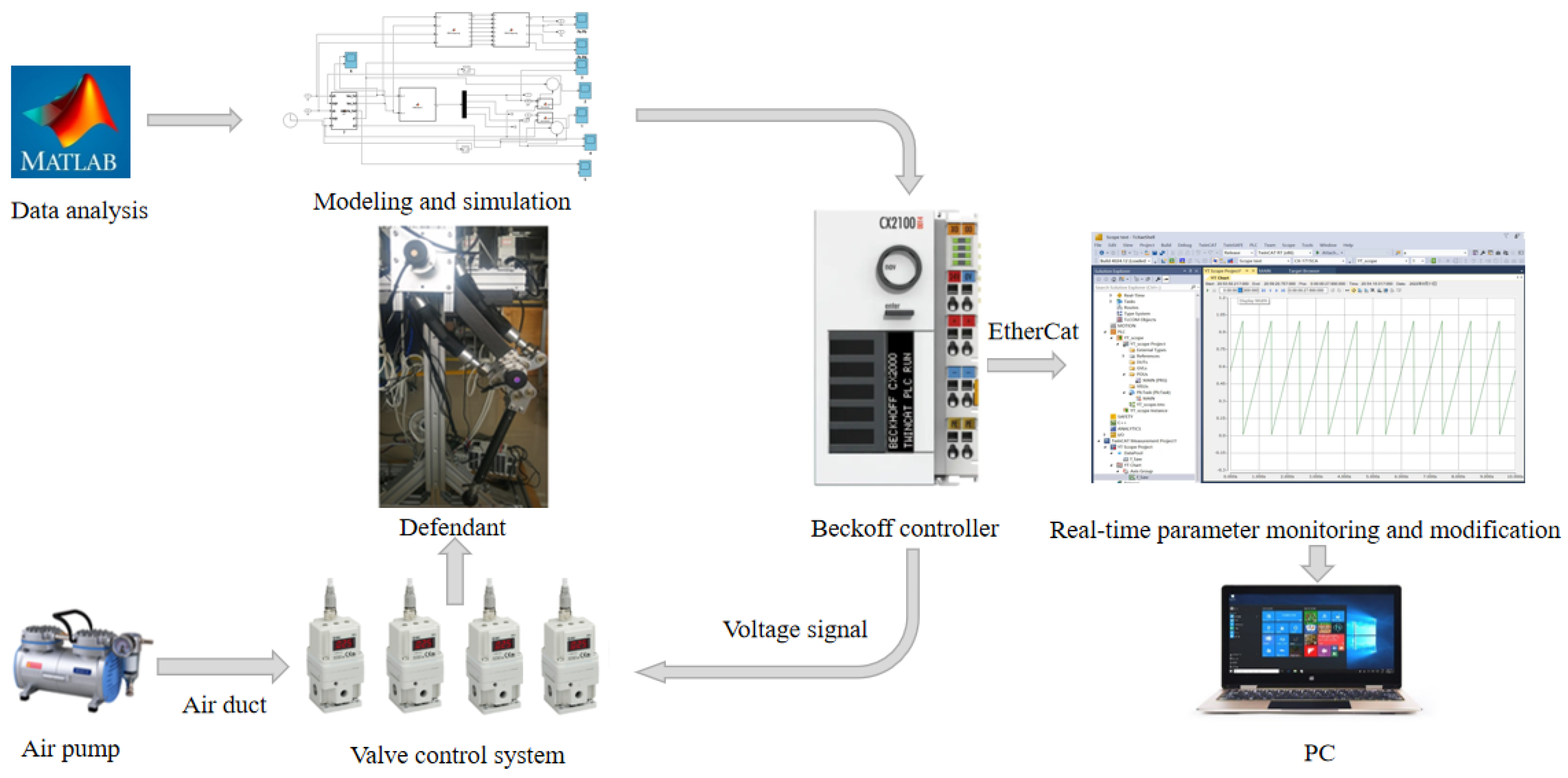
Figure 13 illustrates the proposed experimental platform consists of four major components. First, MATLAB 2024a is employed for data analysis, while the dynamics and control algorithm are established and verified in Simulink 2024a. The validated control laws are subsequently executed by a Beckhoff controller, which communicates with the upper-level PC via EtherCAT, enabling real-time parameter monitoring and online tuning. The controller outputs voltage commands to the valve control system, thereby regulating the air pressure supplied by the compressor and generating the contraction force of the PAMs to drive the PAM-driven biomimetic leg joints system. The resulting joint motion and sensor feedback are transmitted back to the Beckhoff controller, forming a closed-loop control architecture. Overall, the system integrates modeling and simulation, real-time computation, pneumatic actuation, and feedback monitoring into a unified experimental platform, providing a controllable, adjustable, and verifiable platform for PAM-driven biomimetic leg joints system motion control research.

As the leg moves, sensors such as angle encoders measure joint angles. These signals are continuously fed back to the Beckhoff controller, which updates the control algorithm in real time. By adjusting the valve control voltage dynamically, the system maintains the desired trajectory and ensures stable and adaptive pneumatic actuation throughout operation. Note that the proposed controller does not rely on online optimization for system, and all required matrix operations are low-dimensional, making the computational burden compatible with real-time embedded implementation.

Table 6. Technical specifications of key experimental equipment.

Device	Model	Technical Specifications
Hardware Controller	Beckhoff CX2040	Intel Core i7 quad-core @ 2.1 GHz; Microsoft WES7 OS; compact DIN-rail mount; supports real-time control and data processing.
Analog output terminal	Beckhoff EL4008	8-channel analog output; 0–10 V; used to generate proportional-valve command signals.
Analog input terminal	Beckhoff EL3068	8-channel analog input; 0–10 V; 12-bit resolution; used to acquire sensor signals.
Real-time communication	EtherCAT	High-speed real-time communication among the controller and I/O terminals to ensure synchronization.
Joint angle encoder	Single-turn absolute encoder (BRT)	Measurement range: 0–360∘; 12-bit resolution; 24 V DC supply; power-off memory; IP54 protection.
Proportional pressure regulator	SMC ITV2050-212N	Electro-pneumatic regulator; command signal: 0–10 V; gain levels: 0–9.

summarizes the technical specifications of the key equipment used in this study.

To ensure consistency with the simulation study, the uncertainty in the experimental setup is introduced into the mass terms, $m_1\left(t\right)={\overline{m}}_1+\Delta m_1\left(t\right)$ and $m_2\left(t\right)={\overline{m}}_2+\Delta m_2\left(t\right)$, where $\Delta m_1\left(t\right)=0.1sin\left(2\pi t\right)$ and $\Delta m_2\left(t\right)=0.1sin\left(2\pi t\right)$. The desired joint trajectories are defined as time-varying sinusoidal signals and are expressed as follows:

$${\theta }_1=\left(15sin\left(t\right)-45\right){\displaystyle \frac{\pi }{180}},{\theta }_2=\left(15sin\left(t\right)+75\right){\displaystyle \frac{\pi }{180}}.$$

(65)

By solving the joint-to-actuator mapping model in real time, the corresponding desired PAMs force $F_i$ and muscle contraction displacement $x_i$ can be obtained. The joint tracking performance of the PAM-driven biomimetic leg joints system is illustrated by the swing motion curves shown below.

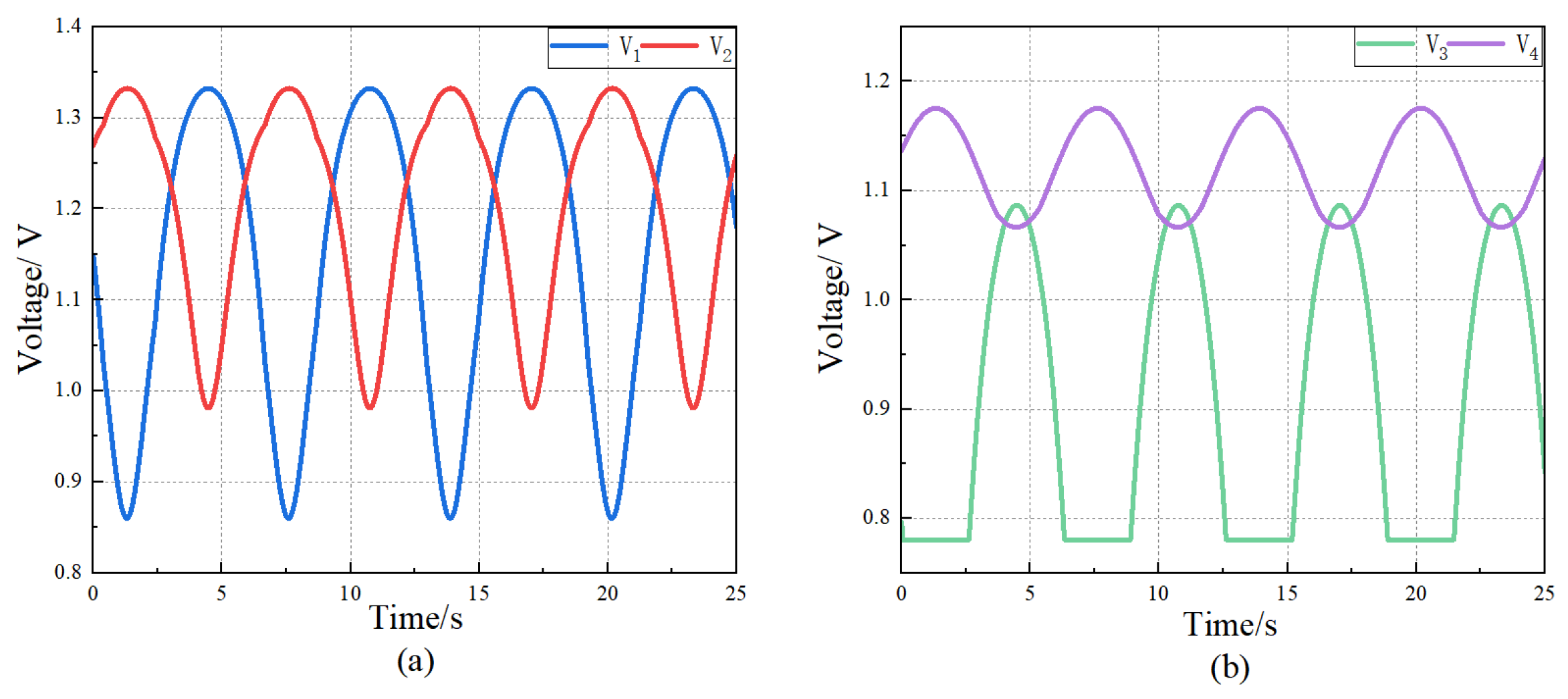
An analog voltage signal was issued via the Beckhoff EL3068 to drive the proportional valve. By adjusting the valve opening, the internal pressure of the PAMs were regulated, enabling control of the muscle’s generated force. Channel-wise voltage outputs are reported in Figure 14 and constitute the raw data for single PAM control. Figure 14a measured voltages of the two antagonistic PAMs at the hip, Figure 14b those at the knee. Apart from the voltage the measured PAM air pressures are reported during experiments. The hip antagonistic air pressures $P_1$ and $P_2$ vary periodically and approximately in anti-phase within $P_1\in [2.23,3.90]\mathrm{bar}$ and $P_2\in [1.80,4.00]\mathrm{bar}$. For the knee joint, the air pressures vary within $P_3\in [2.42,3.22]\mathrm{bar}$ and $P_4\in [1.15,2.98]\mathrm{bar}$. Overall, the air pressure trajectories remain smooth and repeatable over the 30 s tests, indicating stable pneumatic regulation during high-frequency motion.

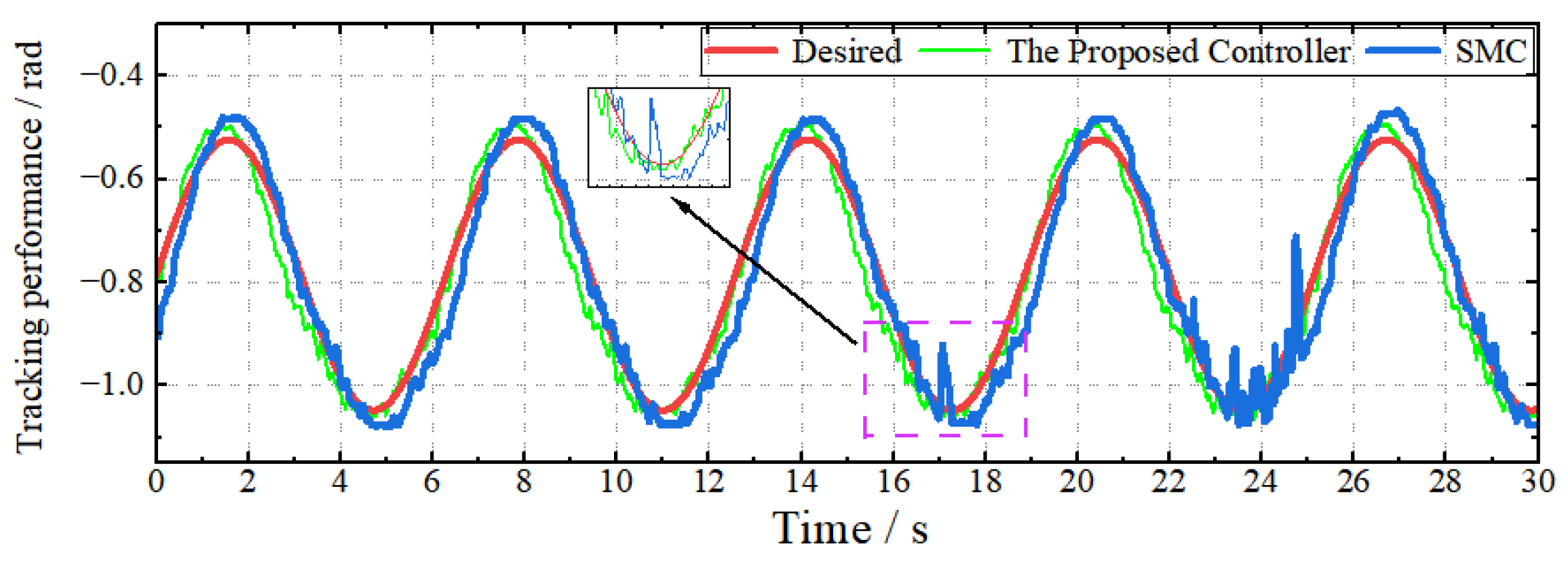
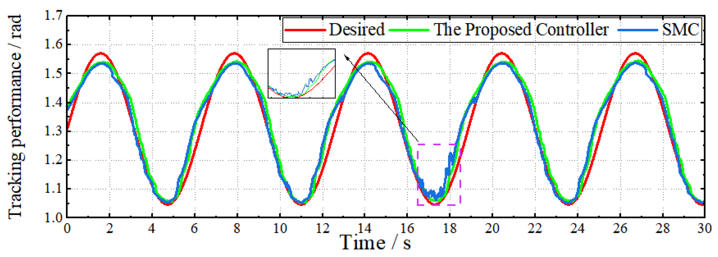
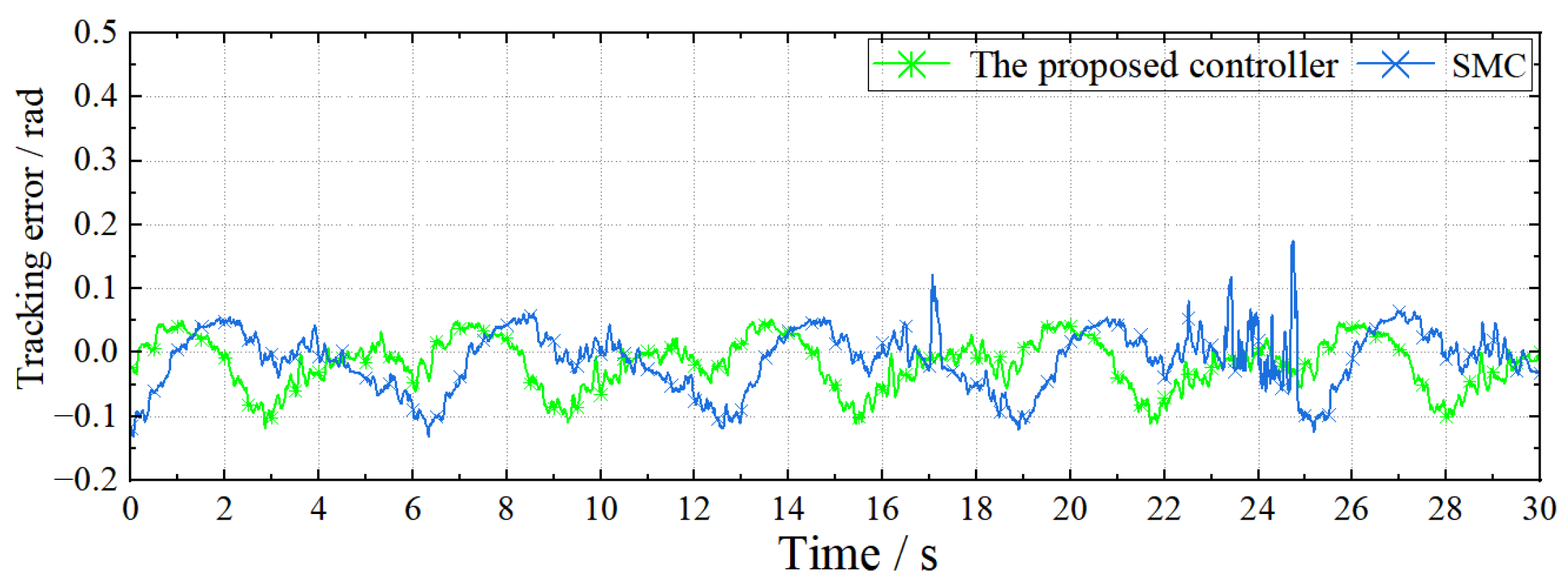
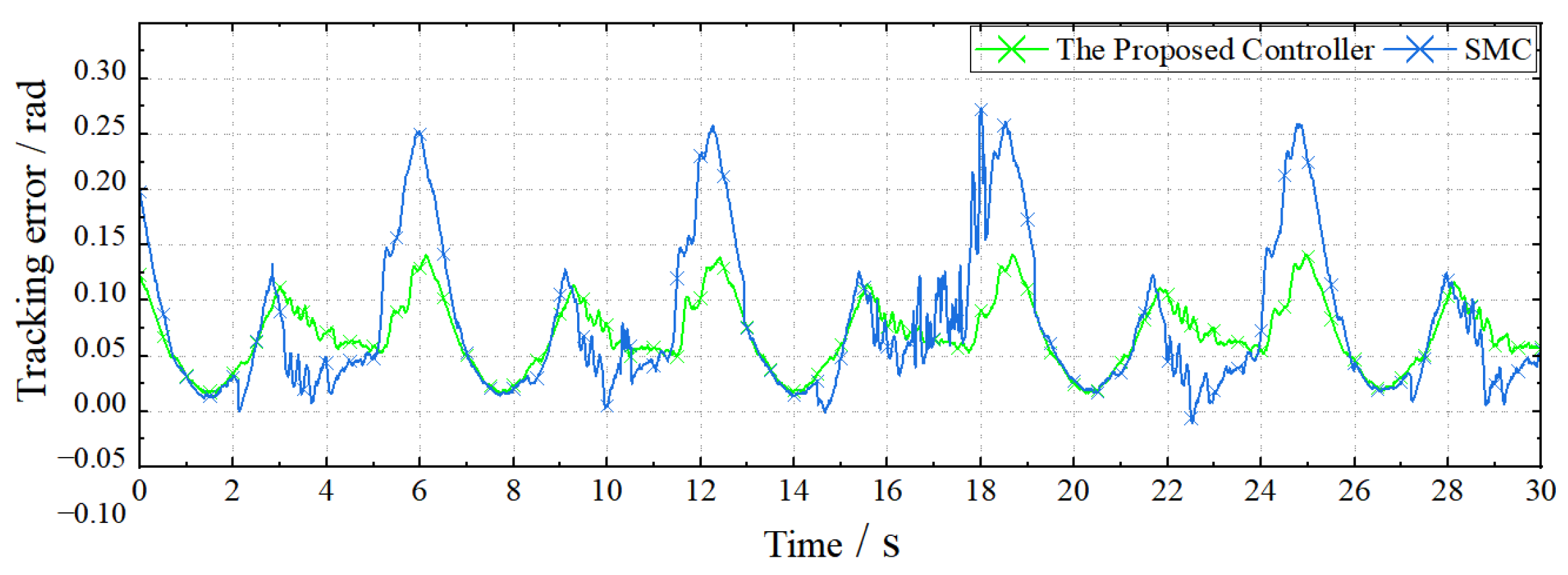
Figure 15 and Figure 16 present the experimental results of joint trajectory tracking under adaptive robust control algorithm and SMC for the hip and knee joints, respectively. In each Figure, the upper subplot displays the actual joint angle overlaid with the desired trajectory, while Figure 17 and Figure 18 show the corresponding tracking errors.

For the hip joint, both controllers successfully follow the periodic desired trajectory. However, adaptive robust control algorithm demonstrates substantially improved tracking precision and smoothness. In particular, adaptive robust control algorithm achieves noticeably smaller error magnitudes near trajectory inflection points, as illustrated in the magnified insets. The tracking error under adaptive robust control algorithm consistently remains within $\pm 0.1$ rad, whereas the SMC exhibits transient spikes exceeding 0.2 rad, highlighting its reduced robustness to dynamic disturbances.

A similar performance advantage is observed for the knee joint. The adaptive robust control algorithm achieves more accurate trajectory tracking with minimal overshoot and steady-state error compared to SMC. The SMC response shows clear deviations during rapid transitions, with errors reaching up to 0.25 rad, where as adaptive robust control algorithm maintains errors predominantly within 0.05 rad. These results confirm that the adaptive robust control algorithm provides superior tracking accuracy, improved robustness, and reduced sensitivity to model uncertainties and high-frequency disturbances, making it well suited for control algorithm of PAM-driven biomimetic leg joints system operating under dynamic motion conditions.

The proposed controller is inherently modular and can be extended from a single leg to multi-leg or full quadruped platforms by applying the same joint-level controller to each actuated DOF. For an n-DOF system, the main online computations include evaluating the nominal dynamics terms and updating the adaptive law. In practice, the required matrix operations remain of moderate size and can be implemented efficiently using precomputed symbolic expressions, recursive dynamics, and lightweight linear-algebra routines. Since the uncertainty compensation is computed locally from measured states and error signals, the algorithm scales approximately linearly with the number of joints when implemented in a per-joint fashion, while cross-leg coupling can be incorporated through the nominal model without changing the overall structure. Moreover, the controller does not require iterative optimization online; thus, its computational burden is suitable for real-time deployment on embedded hardware. With an appropriate sampling rate consistent with pneumatic bandwidth, the control law can be executed within each control cycle on common real-time processors, making the proposed approach a feasible candidate for quadruped locomotion control.

6. Conclusions

This paper proposes an adaptive robust control algorithm to address the intrinsic nonlinearities, time-varying uncertainties, and bandwidth limitations of PAM-driven biomimetic leg joints system. By explicitly embedding second-order trajectory constraints into the control law, the adaptive robust control algorithm enables precise end-effector trajectory tracking while inherently satisfying the system’s dynamic constraints, eliminating the need for complex auxiliary control algorithm. Within this model, adaptive robust control algorithm decomposes the system dynamics into nominal and uncertain components. Unknown disturbances and model uncertainties are mitigated through online parameter estimation, while an adaptive law adjustment mechanism is employed to increase robustness when tracking deviations exceed predefined thresholds. This allows the control algorithm to achieve fast error convergence and maintain stable performance, even in the presence of significant modeling errors and external disturbances. Simulation studies are conducted to evaluate the adaptive robust control algorithm against SMC under trajectory tracking and disturbance rejection scenarios. The results demonstrate clear advantages in terms of steady-state accuracy, disturbance attenuation, and tracking precision. Furthermore, experimental validation on PAM-driven biomimetic leg joints system shows that joint angle tracking errors remain on the order of ${10}^{-2}$ rad during prolonged high-frequency motion, with negligible chattering. The adaptive robust control algorithm exemplifies the integration of adaptiveness and robustness, thereby constituting an advanced control system that is applicable to a wide range of uncertain nonlinear mechanical systems. Its generality and flexibility make it a promising candidate for future intelligent robotic and cyber-physical systems.

Although favorable performance is observed in the tested high-frequency trajectories, the achievable tracking bandwidth is fundamentally constrained by pneumatic actuation, including valve flow limits, air compressibility, pressure dynamics, and transport delays. These factors may degrade performance when the desired motion contains higher-frequency components or rapid torque reversals. Second, the current experimental evaluation primarily focuses on joint-angle tracking; a more comprehensive assessment under broader operating conditions is still needed. Third, extending the proposed approach to human–robot interaction or load-bearing scenarios may introduce additional challenges, such as safety-critical compliance requirements, interaction-force regulation, actuator saturation management, and contact-induced uncertainties, which are not explicitly addressed in the present study. Future work will therefore focus on improving performance under pneumatic bandwidth constraints, reporting additional system-level metrics, and validating the approach in interaction-rich and load-bearing tasks, as well as investigating scalability to multi-leg or full quadruped systems with real-time embedded implementation.

References

1. Buchner, T.J.K.; Fukushima, T.; Kazemipour, A.; Gravert, S.-D.; Prairie, M.; Romanescu, P.; Arm, P.; Zhang, Y.; Wang, X.; Zhang, S.L.; et al. Electrohydraulic Musculoskeletal Robotic Leg for Agile, Adaptive, Yet Energy-Efficient Locomotion. Nat. Commun. 2024, 15, 7634. [Google Scholar] [CrossRef]
2. Zhu, G.; Guo, W.; Chu, S. Bionic Concept and Synthesis Methods of the Biomimetic Robot Joint Mechanism for Accurately Reproducing the Motion Pattern of the Human Knee Joint. Mech. Mach. Theory 2024, 204, 105832. [Google Scholar] [CrossRef]
3. Zielinski, A. Pneumatic Actuating Systems for Automatic Equipment: Structure, Modeling and Control; Springer: Berlin/Heidelberg, Germany, 2006. [Google Scholar]
4. Wang, Q.Q.; Wang, W.; Hao, D.X.; Yun, C. Hysteresis modeling and application of McKibben pneumatic artificial muscles. Chin. J. Mech. Eng. 2019, 55, 73–80. [Google Scholar] [CrossRef]
5. Xie, S.L.; Liu, H.T.; Mei, J.P. Achievements and developments of hysteresis and creep of pneumatic artificial muscles. J. Syst. Simul. 2018, 30, 809–823. [Google Scholar]
6. Yu, J.; Edwards, C. Sliding mode observer design for actuator fault detection. In Advances and Applications in Sliding Mode Control Systems; Edwards, C., Spurgeon, S., Eds.; Springer: Cham, Switzerland, 2017; pp. 123–140. [Google Scholar]
7. Zhou, J.; Krstic, M. Adaptive Predictor Control for Stabilizing Pressure in a Managed Pressure Drilling System Under Time-Delay. J. Process Control 2016, 40, 106–118. [Google Scholar] [CrossRef]
8. Lewis, F.L.; Vrabie, D.; Syrmos, V. Optimal Adaptive Control and Differential Games by Reinforcement Learning Principles; IET Press: London, UK, 2012. [Google Scholar]
9. Zhang, J.; Zhao, R.; Jiao, S. Optimization of robust formation tracking control for traffic cone robots with matching and mismatching uncertainties: A fuzzy-set theory-based approach. Expert Syst. Appl. 2023, 227, 120292. [Google Scholar] [CrossRef]
10. Udwadia, F.E. A new perspective on tracking control of nonlinear structural and mechanical systems. Proc. R. Soc. A Math. Phys. Eng. Sci. 2003, 459, 1783–1800. [Google Scholar] [CrossRef]
11. Udwadia, F.E. A new approach to stable optimal control of complex nonlinear dynamical systems. J. Appl. Mech. 2013, 81, 031001. [Google Scholar] [CrossRef]
12. Chen, Y.-H.; Zhang, X. Adaptive robust approximate constraint-following control for mechanical systems. J. Frankl. Inst B 2010, 347, 69–86. [Google Scholar] [CrossRef]
13. Chen, X.; Zhao, H.; Wang, F.; Zhen, S.; Fang, J. Cooperative Working Performance of a Dual-Arm Robot System Optimised by a Neural Network Adaptive Preset Control. Int. J. Sen. Netw. 2024, 45, 54–65. [Google Scholar] [CrossRef]
14. Huang, K.; Wang, M.; Zhen, S. Udwadia–Kalaba equation based adaptive robust control for two-wheeled inverted pendulum system: Underactuation and uncertainty. Int. J. Control Autom. Syst. 2021, 19, 2420–2430. [Google Scholar] [CrossRef]
15. Liu, X.; Wu, C.; Zhang, S.; Zhou, Y.; Zhen, S.; Sun, H. Nash Game Based Optimal Adaptive Robust Control for Dual-Arm Coordinated Robots. In Proceedings of the 2025 International Conference on Advanced Robotics and Mechatronics, Portsmouth, UK, 1–3 August 2025; pp. 924–929. [Google Scholar]
16. Liu, Z.; Dong, F.; Zhao, X.; Han, J.; Huang, X. Trajectory Generation Strategy for Robots with Redundant DOF Based on the Generalized Udwadia–Kalaba Method: A State-Constrained Natural Solution Approach. J. Frankl. Inst. 2026, 363, 108301. [Google Scholar] [CrossRef]
17. Chen, S.; Han, T.; Dong, F.; Lu, L.; Liu, H.; Tian, X.; Han, J. Precision interaction force control of an underactuated hydraulic stance leg exoskeleton considering the constraint from the wearer. Machines 2021, 9, 96. [Google Scholar] [CrossRef]
18. Ma, C.; Huang, K.; Zheng, J.; Shao, K.; Li, C.; Sun, H. Fuzzy Optimization of Adaptive Integral Terminal Sliding Mode Control for Mechanical Systems with Uncertainties and Disturbances. IEEE Trans. Ind. Electron. 2025, 72, 11822–11831. [Google Scholar] [CrossRef]
19. Yu, R.; Zhao, H.; Zhen, S.; Huang, K. A Novel Approach for 2-Degrees of Freedom Redundant Parallel Manipulator Dynamics. Adv. Mech. Eng. 2017, 9, 1–12. [Google Scholar] [CrossRef]
20. Zheng, Y.; Zheng, J.; Shao, K.; Zhao, H.; Xie, H.; Wang, H. Adaptive trajectory tracking control for nonholonomic wheeled mobile robots: A barrier function sliding mode approach. IEEE/CAA J. Autom. Sin. 2024, 11, 1007–1021. [Google Scholar] [CrossRef]
21. Mylapilli, H.; Udwadia, F.E. Control of three-dimensional incompressible hyperelastic beams. Nonlinear Dyn. 2017, 90, 115–135. [Google Scholar] [CrossRef]
22. Udwadia, F.E. Constrained motion of Hamiltonian systems. Nonlinear Dyn. 2016, 84, 1135–1145. [Google Scholar] [CrossRef]
23. Dong, F.; He, J.; Zhao, X.; Han, J.; Huang, X.; Zhang, X. Analytical Modeling Method for Joint Friction in Harmonic Drive Robot. J. Mech. Sci. Technol. 2024, 38, 3101–3111. [Google Scholar] [CrossRef]
24. Zhao, X.; Cui, Z.; Chew, C.M.; Dong, F. Rendering Compact Formation and Trajectory Tracking for Cyber Unmanned Ground Vehicles. Fundam. Res. 2025, in press. [Google Scholar] [CrossRef]
25. Yin, H.; Yu, D.; Yin, S.; Xia, B. Possibility-Based Robust Design Optimization for the Structural-Acoustic System with Fuzzy Parameters. Mech. Syst. Signal Process. 2018, 102, 329–345. [Google Scholar] [CrossRef]
26. Wu, Q.; Liu, F.; Yin, H.; Huang, J. Constraint-based adaptive robust control for active suspension systems under sky-hook model. IEEE Trans. Ind. Electron. 2021, 69, 5152–5164. [Google Scholar]
27. Chen, S.; Lu, M.; Dong, F.; Liu, H.; Tian, X.; Han, J. Generalized Multiphase Dynamic Modeling and Precision Interaction Force Control of a Walking Lower Limb Hydraulic Exoskeleton. Appl. Bionics Biomech. 2022, 2022, 2801719. [Google Scholar] [CrossRef]
28. Huang, K.; Xia, W.; Shao, K.; Sun, H. Adaptive Sliding Mode Control for Vehicle Active Anti-Roll System Based on Property Adjustable Barrier Function. IEEE Trans. Intell. Veh. 2025, 10, 3124–3133. [Google Scholar] [CrossRef]
29. Liu, X.; Zhen, S.; Sun, H.; Zhao, H. A novel model-based robust control for position tracking of permanent magnet linear motor. IEEE Trans. Ind. Electron. 2020, 67, 7767–7777. [Google Scholar] [CrossRef]
30. Chen, X.; Zhao, H.; Sun, H.; Zhen, S.; Mamun, A.A. Optimal adaptive robust control based on cooperative game theory for a class of fuzzy underactuated mechanical systems. IEEE Trans. Cybern. 2022, 52, 3632–3644. [Google Scholar] [CrossRef] [PubMed]
31. Khalil, H.K. Nonlinear Systems, 3rd ed.; Prentice-Hall: Upper Saddle River, NJ, USA, 2002. [Google Scholar]
32. Chen, Y.H. On the deterministic performance of uncertain dynamical systems. Int. J. Control 1986, 43, 1557–1579. [Google Scholar] [CrossRef]
33. Wang, B.; Wang, Y.; Huang, J.; Zeng, Y.; Liu, X.; Zhou, K. Computed torque control and force analysis for mechanical leg with variable rotation axis powered by servo pneumatic muscle. ISA Trans. 2023, 140, 385–401. [Google Scholar] [CrossRef] [PubMed]
Figure 1. The key control challenges of the PAM-driven biomimetic leg joints system.
Machines 14 00084 g001
Figure 2. PAM-driven biomimetic leg joints system.
Machines 14 00084 g002
Figure 3. (a) Kinematic model of PAM-driven biomimetic leg joints system. (b) Dynamic model of PAM-driven biomimetic leg joints system.
Machines 14 00084 g003
Figure 4. Trajectory tracking of the hip joints.
Machines 14 00084 g004
Figure 5. The knee joints trajectories tracking.
Machines 14 00084 g005
Figure 6. The hip and knee joint errors under the proposed control algorithm and SMC.
Machines 14 00084 g006
Figure 7. Torques of the hip and knee joint.
Machines 14 00084 g007
Figure 8. The adaptive gain parameters.
Machines 14 00084 g008
Figure 9. End effector trajectory tracking errors plot.
Machines 14 00084 g009
Figure 10. (a) PAMs air pressures values of hip joint. (b) PAMs air pressures values of knee joint.
Machines 14 00084 g010
Figure 11. Radar chart of four algorithms on error 1.
Machines 14 00084 g011
Figure 12. Radar chart of four algorithms on error 2.
Machines 14 00084 g012
Figure 13. Schematic design for the experiment platform.
Machines 14 00084 g013
Figure 14. Experimental results of joint output voltage, (a) Hip joint proportional valve input voltage value; (b) Knee joint proportional valve input voltage value.
Machines 14 00084 g014
Figure 15. Experimental results of the hip trajectories tracking.
Machines 14 00084 g015
Figure 16. Experimental results of the knee trajectories tracking.
Machines 14 00084 g016
Figure 17. Experimental results of the hip trajectories tracking errors.
Machines 14 00084 g017
Figure 18. Experimental results of the knee trajectories tracking errors.
Machines 14 00084 g018