Article

Adaptive Traversability Policy Optimization for an Unmanned Articulated Road Roller on Slippery, Geometrically Irregular Terrains

State Key Laboratory of Engines, Tianjin University, Yaguan Rd. 135, Tianjin 300350, China
*
Author to whom correspondence should be addressed.
Machines 2026, 14(1), 79; https://doi.org/10.3390/machines14010079
Submission received: 24 November 2025 / Revised: 31 December 2025 / Accepted: 6 January 2026 / Published: 8 January 2026
(This article belongs to the Special Issue Modeling, Estimation, Control, and Decision for Intelligent Vehicles)

Abstract

To address the autonomous traversability challenge of an Unmanned Articulated Road Roller (UARR) operating on harsh terrains where low-adhesion slipperiness and geometric irregularities are coupled, and traction capacity is severely limited, this paper proposes a Terrain-Adaptive Maximum-Entropy Policy Optimization (TAMPO). A unified multi-physics simulation platform is constructed, integrating a high-fidelity vehicle dynamics model with a parameterized terrain environment. Considering the prevalence of geometric irregularities in construction sites, a parameterized mud-pit model is established—generalized from a representative case—as a canonical physical model and simulation carrier for this class of traversability problems. Based on this model, a family of training and test scenarios is generated to span a broad range of terrain shapes and adhesion conditions. On this foundation, the TAMPO algorithm is introduced to enhance vehicle traversability on complex terrains. The method comprises the following: (i) a Terrain Interaction-Critical Reward (TICR), which combines dense rewards representing task progress with sparse rewards that encourage terrain exploration, guiding the agent to both climb efficiently and actively seek high-adhesion favorable terrain; and (ii) a context-aware adaptive entropy-regularization mechanism that fuses, in real time, three feedback signals—terrain physical difficulty, task-execution efficacy, and model epistemic uncertainty—to dynamically regulate policy entropy and realize an intelligent, state-dependent exploration–exploitation trade-off in unstructured environments. The performance and generalization ability of TAMPO are evaluated on training, interpolation, and extrapolation sets, using PPO, SAC, and DDPG as baselines. On 90 highly challenging extrapolation scenarios, TAMPO achieves an average success rate (S.R.) of 60.00% and an Average Escape Time (A.E.T.) of 17.56 s, corresponding to improvements of up to 22.22% in S.R. and reductions of up to 5.73 s in A.E.T. over the baseline algorithms, demonstrating superior decision-making performance and robust generalization on coupled slippery and irregular terrains.

1. Introduction

UARRs are key equipment in large-scale infrastructure projects, such as road construction and dam embankment. The central articulation steering mechanism grants superior maneuverability compared with rigid vehicles of similar size, but the additional relative rotational degree of freedom also induces high-order, nonlinear coupled dynamics between the front and rear bodies. Furthermore, the smooth steel drum ahead of the joint is purposely designed and, therefore, exhibits intrinsically low tire–ground adhesion. In real operations, rollers frequently work in unstructured environments with low-adhesion surfaces caused by rainfall, watering, or loose soil, coupled with geometric irregularities such as undulations, slopes, trenches, and potholes. When the drum’s inherent low adhesion couples with wet surfaces and terrain slopes, the resulting wet–geometry interaction can easily induce traction loss in the driven drum and severe wheel/drum slip, leading to limited traversability. Understanding and improving the traversability of UARRs on such coupled terrains is thus of both theoretical interest and urgent engineering relevance.
Current research on vehicle traversability over complex terrains can be broadly categorized into three hierarchical layers.

1.1. Low Level: Driveline and Traction Management

Low-level control, such as Traction Control Systems (TCS), provides the foundational capability for traversability. Representative works include slip estimation and control strategies for passenger cars and trucks, as well as electromechanical differential-lock systems that reduce bogging risk on off-road or snow-covered surfaces [1,2,3]. These approaches suppress local slip and maintain traction, which is essential when traversing muddy or sloped regions. However, their efficacy is inherently bound by available adhesion and limited to local, instantaneous responses. Moreover, for hydraulically driven articulated rollers, realizing these low-level actuation capabilities often requires hardware modification, which restricts practical applicability.

1.2. Mid-Level: Motion Planning and Search

Mid-level planning focuses on computing feasible paths that proactively avoid high-risk areas. Search-based algorithms such as RRT and A* have been extended with slip-aware costs, terrain-traversability constraints, and mobility-reliability metrics to reduce bogging risk and planning failure [4,5,6]. Nevertheless, as noted by Gargano, I.E. [7] and Wang, N. [8], these methods are highly sensitive to prior knowledge and real-time perception of terrain parameters, such as soil properties and adhesion. In wet–geometry-coupled scenarios, where wheel–ground interaction is complex and physical parameters are time-varying and difficult to sense accurately, such priors are often insufficient. Another line of work codifies human recovery heuristics into expert policy libraries or action primitives and searches online for effective recovery sequences [9,10]. While effective in specific settings, these methods are highly sensitive to prior terrain knowledge and perception accuracy. In wet–geometry-coupled scenarios, where wheel–ground interaction is complex and physical parameters are time-varying and difficult to sense, such prior information is often insufficient.

1.3. High Level: Learning-Based Decision-Making

Reinforcement learning (RL) offers a new paradigm for traversability on coupled terrains due to its ability to adapt to unknown dynamics, handle time-varying constraints, and perform end-to-end optimization. Sánchez, M. et al. [11] combined curriculum learning with RL to learn traversing strategies in unstructured off-road environments, representing a typical terrain-aware reward-shaping and curriculum-learning framework. Xu, T. et al. [12] built an end-to-end RL system and a benchmark for “steep slope–boulder–gully” vertical challenge terrains to evaluate wheeled platforms. Siva, S. et al. [13] proposed a reflexive terrain perception and adaptation framework that produced consistent, stable navigation across multiple unstructured terrains. Overall, RL has emerged as a promising mainstream approach for extreme-terrain traversability.
However, directly applying standard RL to autonomous traversability of UARRs on wet–geometry-coupled terrains faces two core challenges:
  • Reward design. The task reward is naturally sparse and deceptive, easily causing credit-assignment difficulties and training stagnation. As shown by Devidze, R. et al. [14], a lack of effective reward shaping can markedly slow learning or even prevent convergence.
  • Exploration–exploitation trade-off. Maximum-entropy RL algorithms (e.g., SAC [15]) encourage exploration via a temperature parameter. To improve adaptivity, several works learn or schedule this parameter, or otherwise modulate exploration, including meta-gradient temperature tuning and target-entropy annealing in SAC, value-conditional state-entropy exploration, uncertainty-driven bonuses for generalization, and adaptive entropy-regularization frameworks in multi-agent RL [16,17,18,19,20]. While effective on standard benchmarks, these schemes typically rely on a single generic signal (state entropy or value uncertainty) and do not explicitly incorporate a terrain’s physical difficulty or task-progress information into the entropy schedule, which limits their task-specificity in strongly heterogeneous, wet–geometry-coupled terrains.
From a control-architecture perspective, the proposed RL approach is positioned as a high-level traversability decision layer that complements, rather than replaces, classical model-based controllers. Specifically, while Model Predictive Control (MPC) is preferable for precise path tracking when terrain dynamics can be reliably modeled and a reference path is available, the blind mud-pit scenarios considered here present a fundamental challenge: strongly non-uniform and unobservable soil parameters render online model identification unreliable. Consequently, a model-free policy—trained offline in a high-fidelity Simscape environment and deployed online as a lightweight decision module—emerges as a practical choice for handling the coupling between planning and control under extreme uncertainty.
To address autonomous traversability of UARRs on terrains characterized by coupled low adhesion and geometric irregularities, this paper proposes TAMPO within an RL framework. The novelty of this work is three-fold:
  • A component-based multi-physics simulation platform is developed for an articulated road roller operating on parameterized mud-pit terrains. The platform closely matches the real vehicle and generates a broad family of scenarios by varying adhesion, pit depth, and geometric shape, providing a physically grounded benchmark and training/test sets for traversability studies.
  • A TICR function is designed that jointly encodes task-progress signals and physically grounded terrain attributes (adhesion, sinkage, and slope). This goes beyond existing terrain-aware reward shaping by explicitly targeting mud-pit traversability and alleviating credit-assignment difficulties under sparse and deceptive rewards.
  • A context-aware adaptive entropy-regularization mechanism is developed, in which the policy temperature is an explicit state-dependent function of terrain physical difficulty, task-execution efficacy, and epistemic value uncertainty. This contrasts with meta-gradient, state-entropy, and uncertainty-only schemes that rely on a single generic signal and ignore task-specific terrain context, enabling more robust exploration–exploitation balancing on strongly heterogeneous, wet–geometry-coupled terrains.
The remainder of this paper is structured as follows: Section 2 first analyzes a representative bogging incident and, based on this, builds the simulation environment and physical models used to study the general traversability problem. Section 3 details the proposed TAMPO algorithm. Section 4 presents simulation training and generalization tests to validate the approach’s effectiveness. Section 5 concludes the paper. Section 6 discusses directions for future work.

2. Simulation Platform

2.1. Representative Case

When an articulated compaction roller operates on unpaved ground, the core bottleneck to autonomous traversability is traction failure induced by the coupling of low-adhesion surfaces and local geometric irregularities.
A typical and severe failure mode is illustrated in Figure 1: The roller experiences high slip on a wet mud road, rapidly excavates a local pit, and becomes immobilized. This bogging scenario precisely epitomizes the wet–geometry coupling problem and encapsulates its two essential factors:
  • The low-adhesion property inherent to wet soil.
  • The geometric irregularity is characterized by the localized, steep slopes formed by the depression.
Under such coupled conditions, insufficient tractive effort is produced to overcome the gravitational component due to the slope and the rolling resistance due to the mud, leading to traction loss and loss of mobility, which severely constrains both efficiency and safety on site. Motivated by this observation, the above failure mode is generalized in the terrain construction: a parameterized mud pit is selected as the standard physical model and simulation carrier for studying this generic traversability problem, so as to provide a controllable testbed for the autonomous traversability strategies developed in the sequel.

2.2. Construction of the Simulation Platform

2.2.1. Overview of the Simulation Method

A vehicle-dynamics simulation platform is indispensable for developing, validating, and iterating algorithms. While commercial tools—such as CarSim [21,22] and CarMaker [23,24] for passenger and light vehicles, or TruckSim [25] and TruckMaker [26] for heavy vehicles—offer mature solutions for standard vehicles, an integrated, high-fidelity environment tailored specifically to articulated road rollers remains scarce. Consequently, researchers often resort to multi-software co-simulation (e.g., ADAMS combined with AMESim) [27]. However, this heterogeneous coupling introduces considerable challenges. These include model integration complexity, data inconsistency, numerical instability, computational overhead, and deficient real-time performance.
To overcome these limitations, a component-based physical network modeling paradigm is adopted [28,29]. The core idea involves connecting component models of physical entities through standardized, energy-conserving ports. This enables unified modeling and solution of multiple physical domains—multibody dynamics, hydraulic actuation, and wheel–ground interaction—within a single Differential-Algebraic Equation (DAE) framework. This noncausal, object-oriented paradigm emphasizes physical topology over signal flow. This approach ensures physical consistency while markedly improving model reusability, maintainability, and test efficiency. The paradigm’s advantages are summarized as follows:
  • Structured physical representation and high reusability. Each component encapsulates its internal constitutive laws and interacts solely via standardized power ports. This modular structure renders the assembly and reconfiguration of subsystems (e.g., articulated frame, drum/wheels) intuitive, akin to physical prototyping. Crucially, changes in system topology or parameters do not necessitate rewriting low-level solver code, yielding high flexibility.
  • Unified solution of strongly coupled multi-physics. All components are numerically integrated within a single DAE solver. This intrinsically supports stable and consistent simulation of highly nonlinear, strongly coupled phenomena. Examples include valve-controlled hydraulics, line compressibility, and nonlinear wheel–ground contact/friction. Furthermore, it avoids interface errors common in co-simulation, which typically arise from cross-platform time-step synchronization and data interpolation, thereby improving numerical robustness and physical fidelity.
  • Seamless co-simulation of control and physics. The physical model is co-simulated with control algorithms within the same environment (MATLAB/Simulink R20225b), forming a closed-loop testbed. Physical and control quantities share a unified time base and data space. This streamlines controller/decision parameter calibration, observer design, and sensitivity analysis, facilitating a smooth transition from Model-in-the-Loop (MIL) to Real-Time Simulation and Hardware-in-the-Loop (HIL) testing.

2.2.2. Overview of the Simulation Platform

Overall Model Architecture
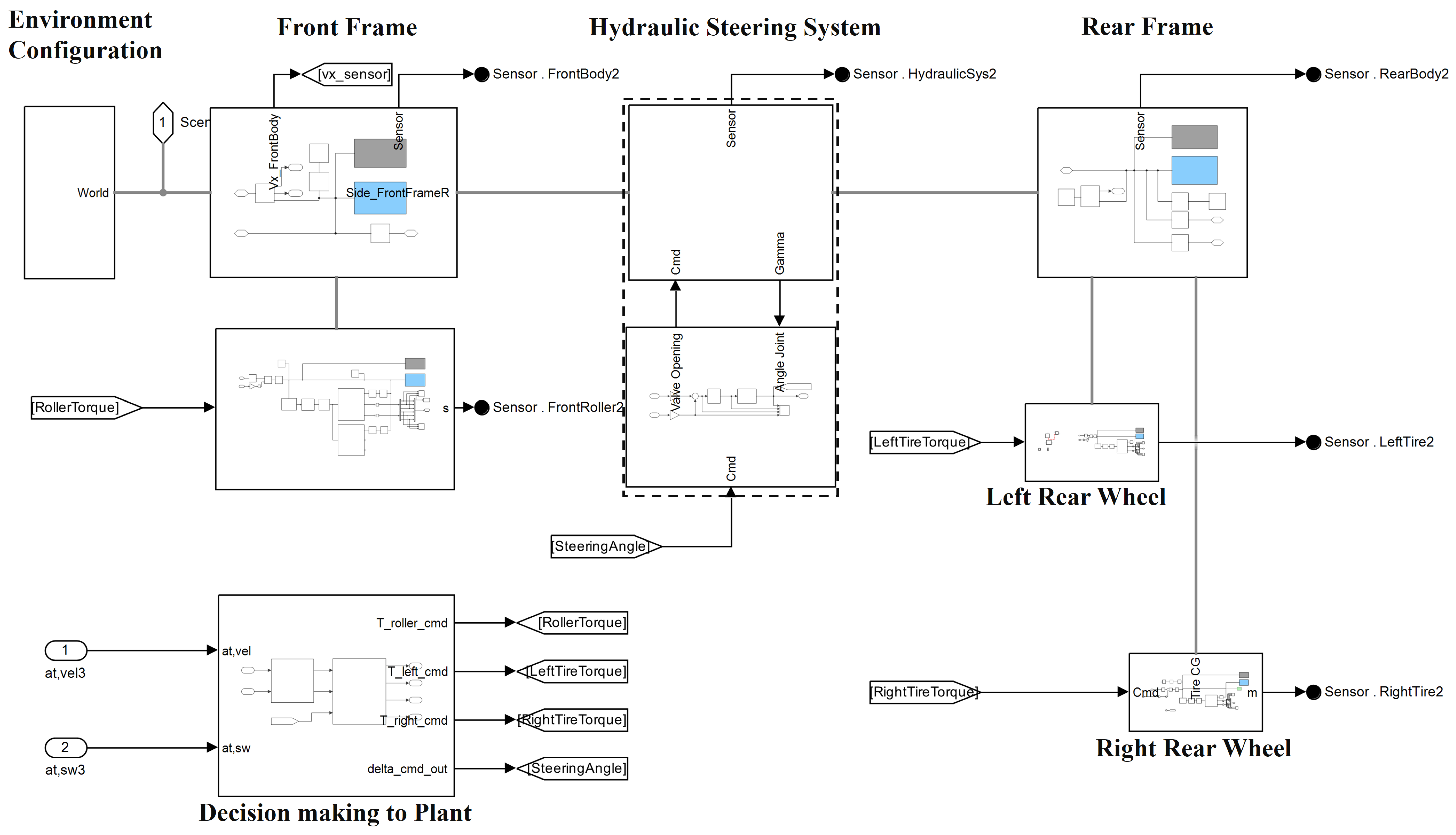
The simulation platform (Figure 2) is structured around three integrated parts: (i) the vehicle subsystems, (ii) a global environment configuration module, and (iii) the command-mapping and execution interface. The vehicle model specifically comprises the following subsystems: the drum, the front frame, the left and right rear wheels, the rear frame, and the hydraulic steering unit. The global environment module is responsible for specifying the inertial reference frame, the gravity field, the solver type, and the simulation step size. In closed-loop experiments, the physical model functions as the plant, receiving action commands from the policy optimizer. Its state outputs are simultaneously streamed to a 3-D visualization module for scene rendering and results analysis.
All subsystems are assembled strictly according to the real machine’s physical topology. The front frame connects to the hydraulic steering unit (via two cylinders) at the central articulation joint. The rear frame is connected to the opposite ends of these cylinders and to the steering linkages. The drum is mounted to the front frame via a single revolute joint. Model parameters were determined through a combination of product datasheets, manual measurements, analytical calculations, and offline identification. The principal parameters are summarized in Table 1.
Hydraulic Steering Subsystem
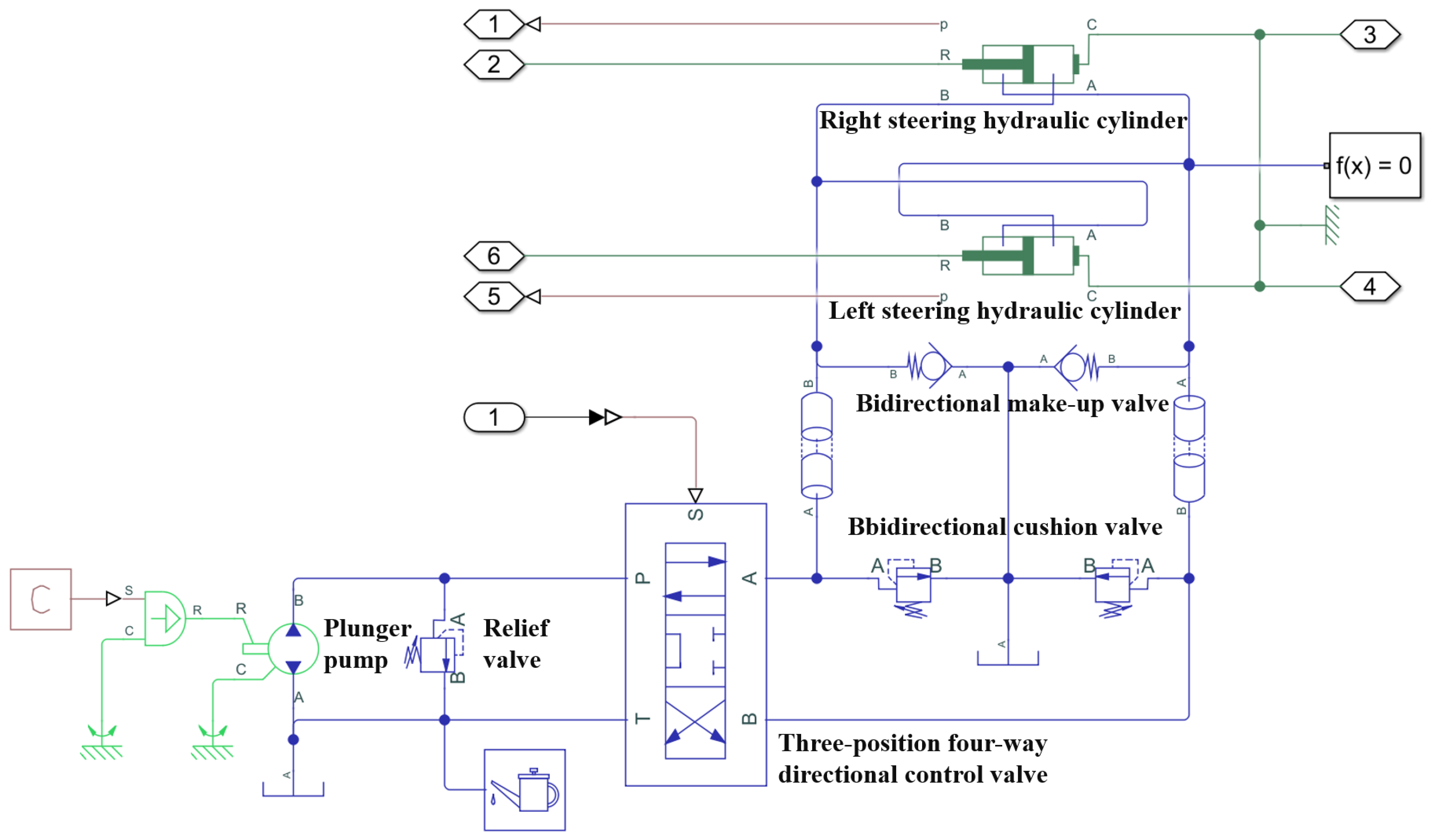
The steering motion of the UARR is actuated by a closed-loop hydraulic system. Mechanical power is converted into hydraulic power, which ultimately translates into calibrated push–pull forces at two symmetric steering cylinders. This arrangement generates the required steering moment for relative rotation between the front and rear frames. The subsystem, illustrated in Figure 3, is organized into the following key components:
  • Power supply and control valve. A plunger pump is modeled as the pressure source, emulating the engine output. A three-position, four-way proportional directional valve serves as the core control element; it meters and reverses the flow delivered to the left and right cylinders according to external command signals.
  • Bilateral cylinder actuators. Two symmetrically arranged double-acting cylinders are modeled as the primary steering actuators. They convert hydraulic energy into mechanical work at the articulation joint. To ensure physical fidelity, key geometric and operating parameters—specifically the bore, rod diameter, and stroke/travel range—are calibrated using data from the real vehicle (see Table 2).
  • Auxiliary and protection elements. The model also integrates auxiliary components essential for physical realism and numerical robustness. These include a relief valve to cap the maximum pressure, make-up valves to mitigate cavitation, and snubbers or accumulators to attenuate pressure spikes.
In this manner, the model accurately reproduces the full nonlinear response chain, from control input to steering moment output, providing a high-fidelity steering-torque source for the whole-vehicle dynamics simulation.
Wheel–Terrain Simulation Model
(1)
Wheel–ground contact model
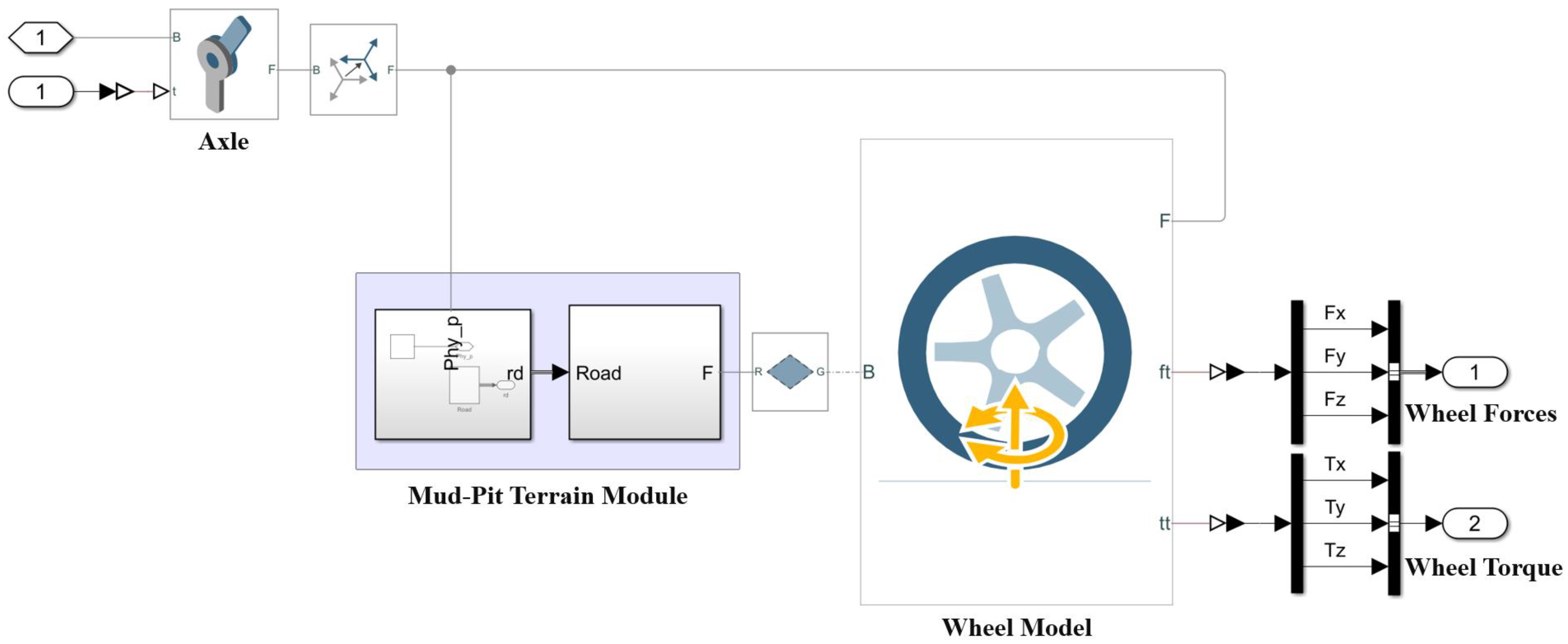
The wheel subsystem (Figure 4) is designed to compute the interaction forces and moments at the wheel–terrain interface in real time. Key parameters for both the front drum and the rear wheels are summarized in Table 3. A local terrain-mapping and contact-force reconstruction scheme is employed to accurately reproduce the dynamic excitation caused by the parameterized mud-pit surface. The workflow is as follows:
  • Terrain query. The world coordinates of the wheel center are used to query the local pit-surface height, the surface normal vector, and the position-dependent friction (adhesion) field.
  • Local frame alignment. A local ground frame is instantiated based on the queried normal vector. The wheel–ground contact is then geometrically aligned with this frame to inject the terrain’s geometric excitation.
  • Relative motion decomposition. The linear and angular velocities at the contact patch (provided by the multibody solver) are decomposed into normal and tangential components. Longitudinal slip and sideslip are subsequently computed from the tangential components.
  • Effective adhesion evaluation. The terrain cells covered by the instantaneous contact patch are aggregated using area weighting to obtain a time-varying effective adhesion coefficient.
  • Contact-force reconstruction. Normal support and tangential friction forces are calculated using equivalent normal stiffness/damping along with the effective adhesion. The tangential force component is constrained by the friction limit.
  • Force–structure feedback. The reconstructed tri-axial forces and moments are applied back to the wheel and frame for the next multibody integration step. These forces are simultaneously exported to the virtual-sensor bus.
(2)
Parametric Mud-Pit Terrain
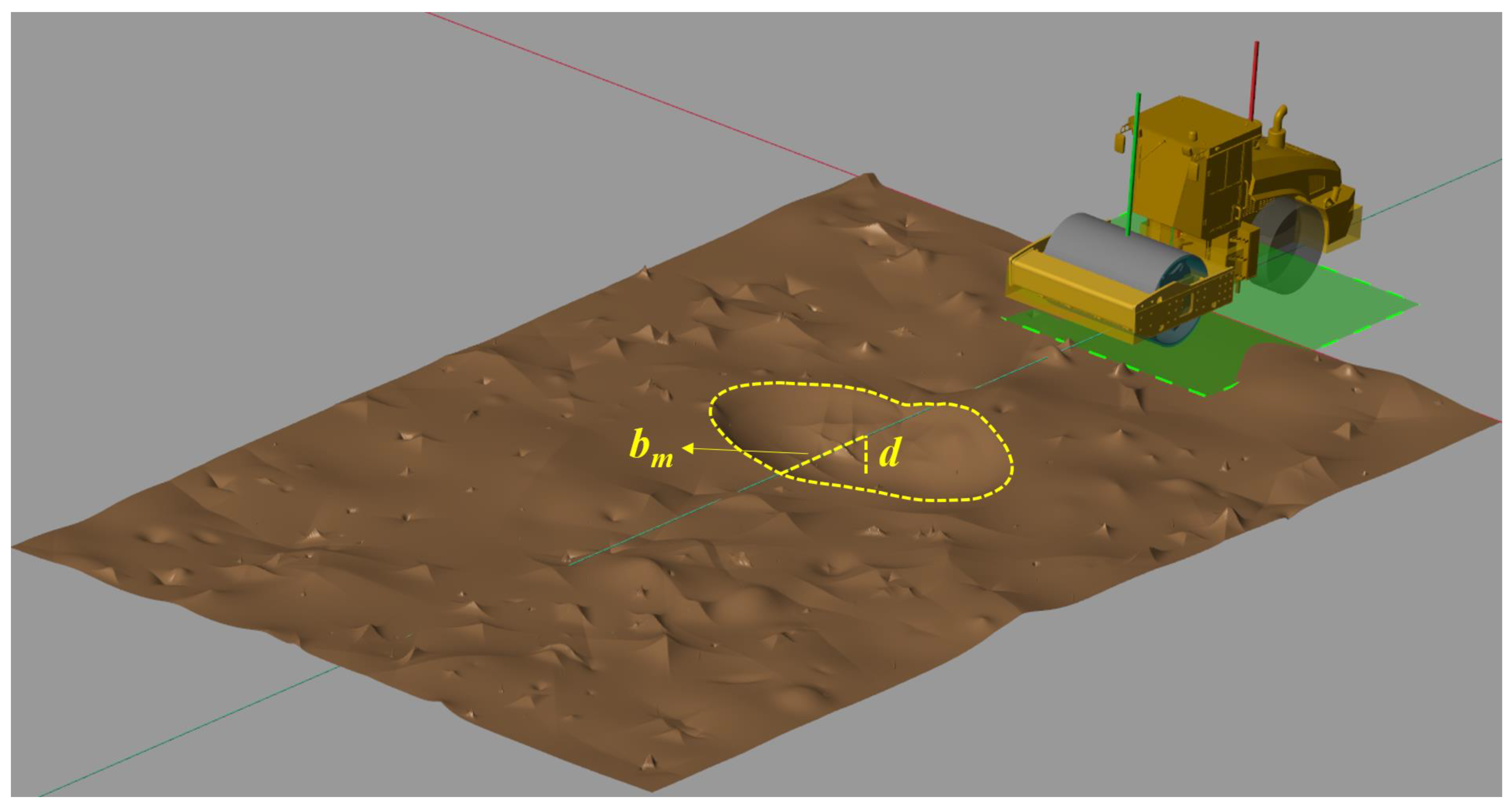
To support policy training and generalization tests, a controllable parametric mud-pit environment was constructed based on field observations of real pits (cf. Figure 1). The environment comprises a geometric description of the pit surface and parameters capturing its mechanical properties.
  • Geometry
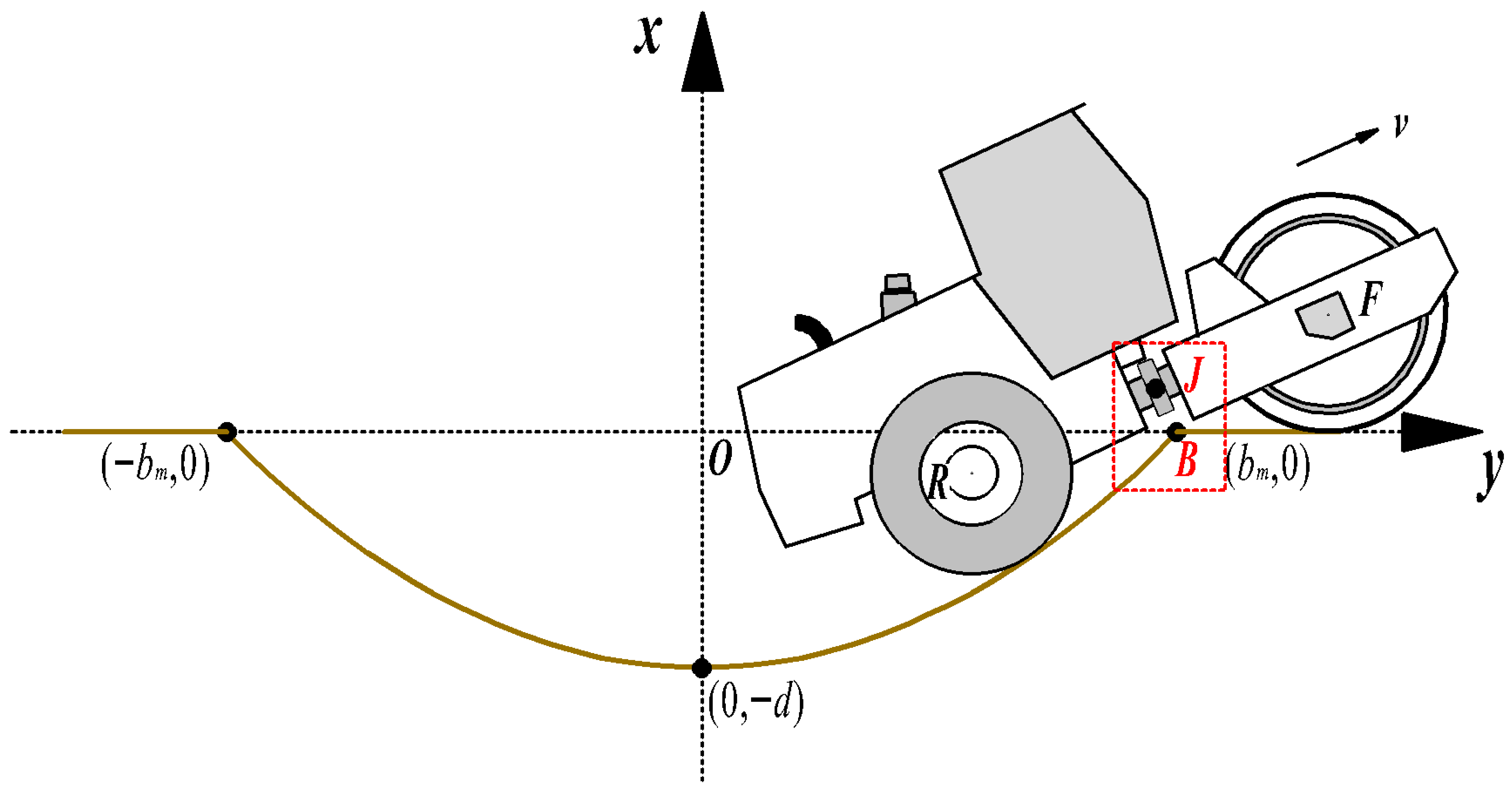
The mud pit is modeled as a parametric surface featuring elliptical level curves and parabolic cross-sections. The shape is uniquely determined by the pit-bottom center ( x c , y c ) , the maximum depth d , and the semi-axes of the elliptical rim, a m and b m . This representation compactly captures the geometry of the bowl-/dish-shaped pits commonly found in practice. The surface height z ( x , y ) is given by the following:
z ( x , y ) = d ( x x c ) 2 a m 2 + ( y y c ) 2 b m 2 d .
Here, d > 0 denotes the maximum pit depth at the center ( x c , y c ) , and the level sets of z ( x , y ) are ellipses with semi-axes a m and b m . Consequently, the mud pit forms a smooth bowl-shaped depression that is wider along the b m direction and narrower along the a m direction, with cross-sections in the x - and y -directions taking simple parabolic profiles.
  • Physical properties (spatially varying adhesion)
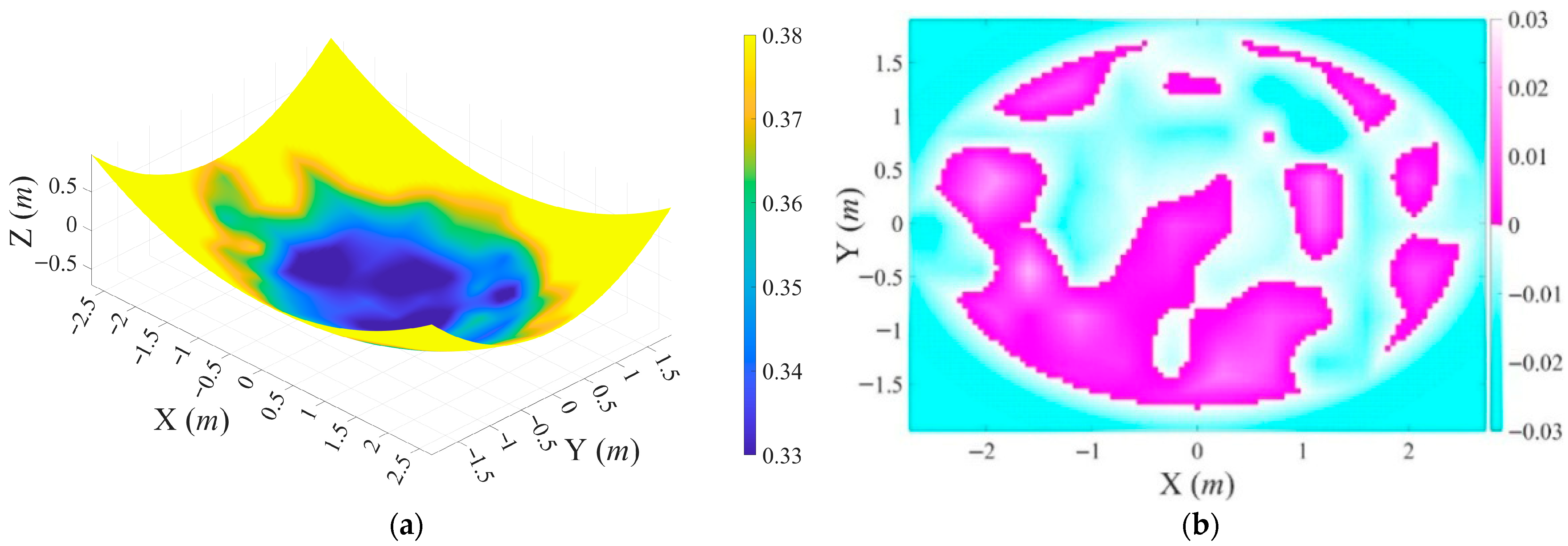
To reproduce the heterogeneity of wet, slippery soil, the adhesion coefficient is modeled as a superposition of three components. Figure 5 illustrates a pit with μ b a s e = 0.35 and the corresponding adhesion increment field:
 (i)
Nominal adhesion: μ n v [ 0.35 ,   0.70 ] defining the baseline friction level.
 (ii)
Deterministic gradient: This term reflects the positional dependence (equivalently, depth) of the surface, where water accumulation toward the pit bottom lowers adhesion in deeper regions, and adhesion increases toward the rim.
 (iii)
Stochastic heterogeneity: This is generated via Perlin noise [30,31] to form spatially correlated patches on top of the gradient, emulating random local variability.
  • Feasibility constraints and discretization
Arbitrary combinations of d , a m , b m may produce trivial or physically infeasible training cases. Two physics-based constraints are therefore imposed to guarantee meaningful, solvable scenarios and improve training efficiency.
 (i)
Traction-feasibility boundary.
To guarantee that a generated scene is theoretically solvable, the roller is required to possess sufficient maximum tractive capacity along the least-steep ascent path—i.e., along the major axis of the elliptical rim ( φ s = ± π / 2 ) —to overcome the gravitational grade resistance.
Assume the horizontal projection of the pit bottom center is located at ( x , y ) = ( 0,0 ) . Introduce the polar parametrization ( x , y ) = ( r s s i n φ s ,   r s c o s φ s ) , where r s 0 denotes the radial horizontal distance from the pit center and φ s is the horizontal azimuth. The norm of the surface gradient z derived from the pit profile in Equation (1) is thus obtained as a function of ( r s , φ s ) :
g c , t = 2 d r s sin 2 ( φ s ) a m 4 + cos 2 ( φ s ) b m 4 .
The admissible climbing sector is the forward fan π / 2 φ s π / 2 , with the y -axis corresponding to φ s = 0 .
Under the traction-limit assumption, the maximum climbable elevation along the direction φ s at distance r s , denoted h m a x ( φ s ) , is given in Equation (3):
h max ( φ s ) = μ x 2 sin 2 ( φ s ) a m 2 + cos 2 ( φ s ) b m 2 4 d sin 2 ( φ s ) a m 4 + cos 2 ( φ s ) b m 4 .
As implied by Equation (3), when φ s = ± π / 2 (ascent projected along the major semi-axis), the local slope is the gentlest and the theoretical climb height is the largest; when φ s = 0 (along the minor semi-axis), the slope is steepest and the theoretical climb height is the smallest.
During scenario design, it is required that a feasible ascent to the rim exists along the least-steep direction; equivalently, the constraint in Equation (4) must be satisfied:
h max ( ± π 2 ) = μ x 2 4 d a m 2
 (ii)
Geometric no-interference boundary.
To avoid articulation-joint grounding during ascent—especially along the minor axis ( φ s = 0 ), where the slope is steepest—the depth d must remain below a maximum allowable depth d m a x dictated jointly by the vehicle geometry and rim size (see Figure 6):
d max ( 0 ) = b m 2 4.066 b m 3.42
Accordingly, admissible values of a m ,   b m , and d are selected under the above two constraints.
  • Scenario set generation
    The parameter space is discretized as follows:
    (i)
    Adhesion coefficient set S μ : Eight nominal values are selected within [ 0.35 ,   0.70 ] with a step size of 0.05.
    (ii)
    Rim-size set S b m : Nine representative short semi-axis values are sampled. These values are linked to the drum geometry (drum length B = 2.13   m , diameter D drum = 1.6   m ), S b m = { 1,1.5,2 , 2.5,3 , 3.5,4 , 4.5,5 }   m .
    (iii)
    Depth set S d : The dimensionless sinkage coefficient s d = d / D drum is used to classify pits into shallow [ 0.05,0.2 ] , medium ( 0.2,0.4 ] , and deep ( 0.4,0.6 ] ranges; Twelve representative depths are sampled, S d = { 0.08,0.16,0.24,0.32,0.40,0.48,0.56,0.64,0.72,0.80,0.88,0.96 }   m .
The Cartesian product Ω =   S μ × S b m × S d   = 864 defines the training set. All parameters are normalized to remove unit-scale disparity. A 3-D view of the environment and a labeled parametric pit is shown in Figure 7.
Validation of the Simulation Platform
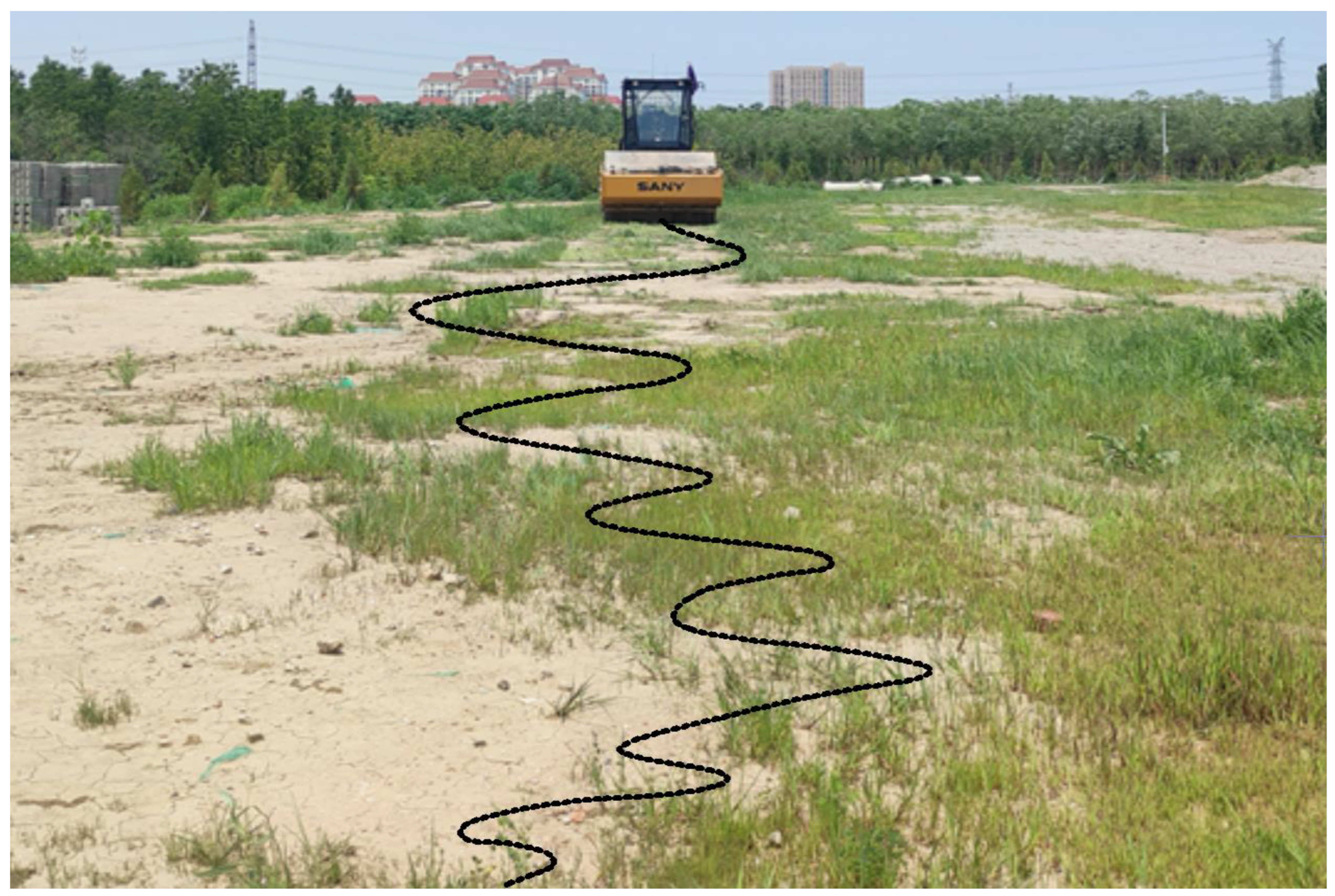
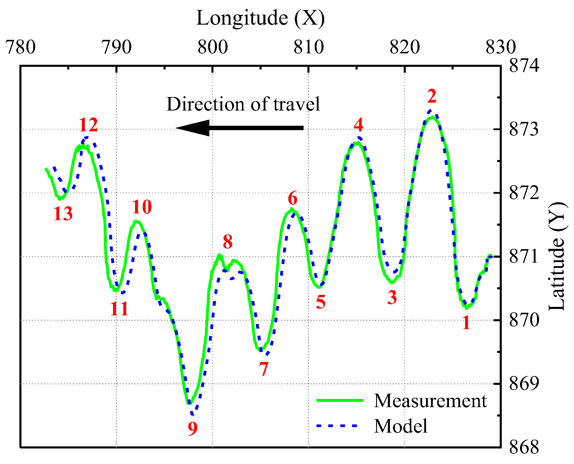
To evaluate the fidelity of the simulation platform’s dynamic response, this section conducts a comparative study between real-vehicle tests and simulations of an articulated road roller performing large-amplitude “S”-shaped steering maneuvers. As shown in Figure 8, the roller travels on a dry soil road at a constant target speed of 2.5 km/h, while the steering wheel is operated to execute multiple large-amplitude alternating steering inputs (peak magnitude ±1500°). During the experiment, the combined navigation system records key dynamic variables, including the drum center-of-mass position, velocity, yaw angle, and steering-wheel angle; the drum lateral sideslip angle is further obtained indirectly from the velocity information. In the simulation, the measured steering-wheel angle sequence is applied to the model as an open-loop control input, and the simulated vehicle speed is set to match the recorded test speed to ensure a consistent basis for comparison.
Figure 9 provides a qualitative comparison between the measured and simulated driving trajectories. The two paths show a high degree of overlap in overall shape, turning locations, and lateral deviation amplitude. Table 4 summarizes the peak lateral positions at the 13 turning points. For each turn, the absolute error e i = y i sim y i meas is normalized by the total lateral excursion Δ y = m a x ( y meas ) m i n ( y meas ) to obtain the relative error e i / Δ y . Although the open-loop use of the measured steering input leads to some accumulated drift over time, the average normalized peak error remains as low as 2.51%, and the coefficient of determination ( R 2 ) between the measured and simulated trajectories reaches R 2 = 0.985 , indicating an excellent goodness of fit and demonstrating high fidelity of the simulation platform.
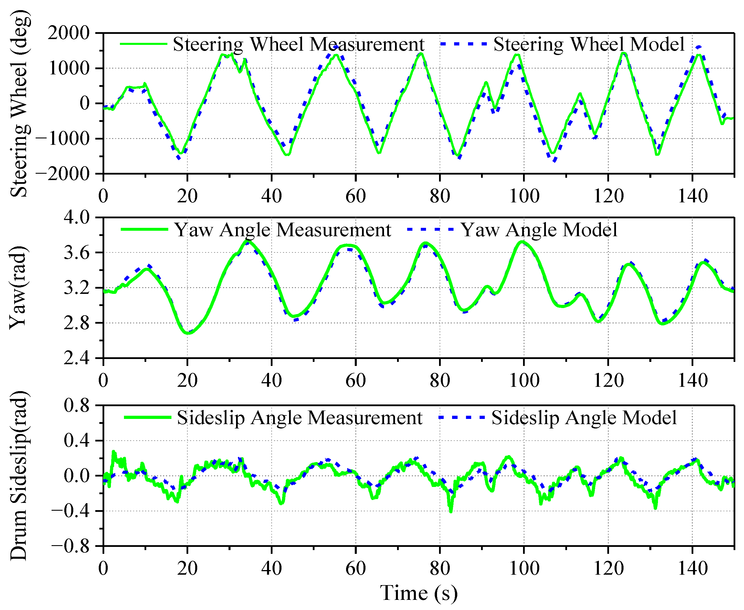
Figure 10 compares the measured and simulated time histories of the steering-wheel angle, yaw angle, and drum-CG sideslip angle during the continuous S-shaped steering maneuver. The simulated responses closely track the measurements in both amplitude and phase. The coefficients of determination R 2 for the steering-wheel angle, yaw angle, and sideslip angle are 0.953, 0.984, and 0.704, respectively, demonstrating high simulation accuracy. The lower R 2 for the sideslip angle is mainly attributed to its small magnitude and indirect estimation from velocity measurements, which makes it more sensitive to navigation noise and wheel–ground slip modeling errors; nevertheless, the simulated sideslip angle reproduces the overall measured trend. These results confirm that the simulation platform reliably captures the multi-DOF coupled dynamics of the roller under complex, large-amplitude S-shaped steering.
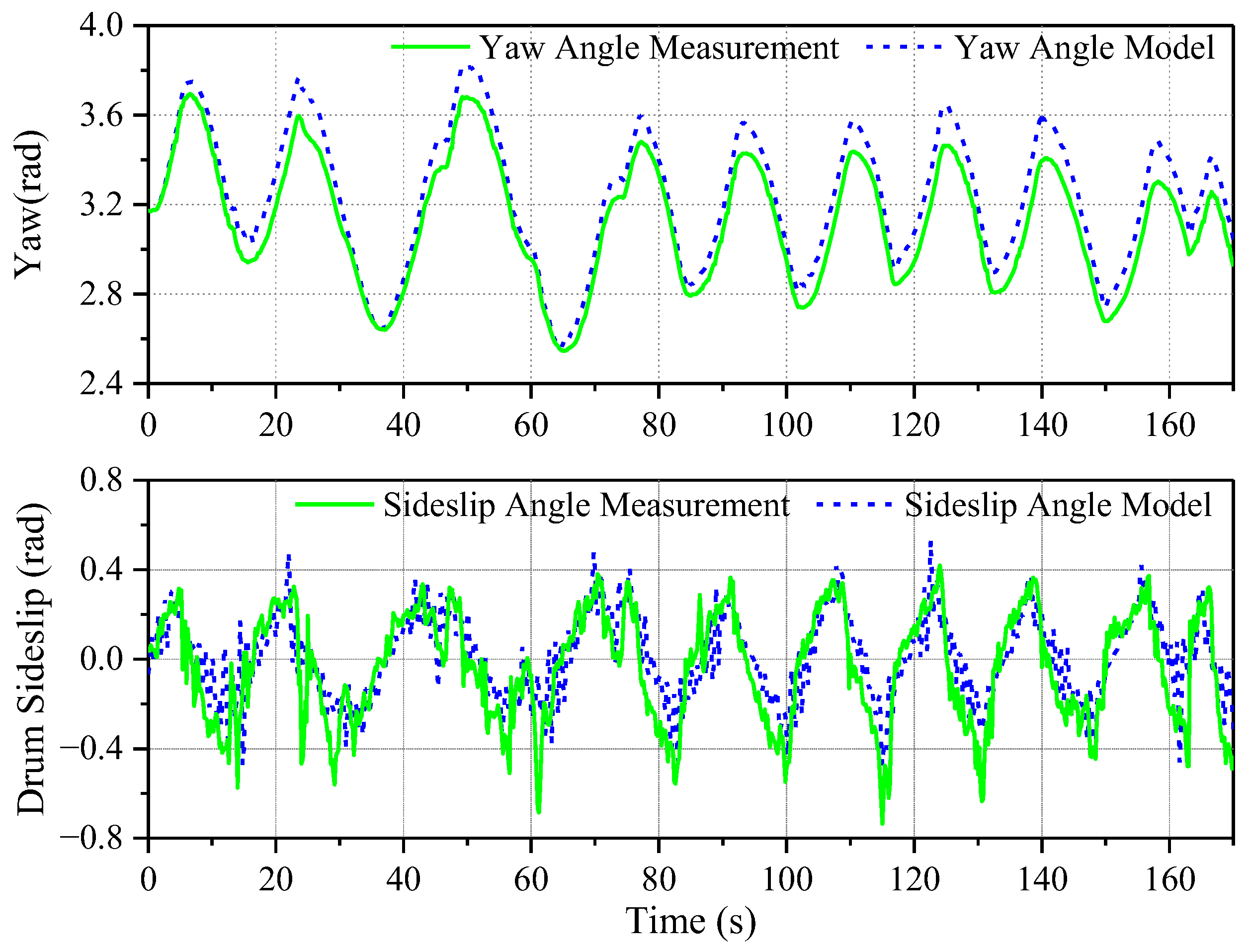
To further assess the predictive accuracy of the simulation platform under wet soil conditions, the continuous S-shaped steering test was repeated on a wet soil road surface after rainfall. Figure 11 compares the simulated and measured responses, where the coefficients of determination for the yaw angle and drum-CG sideslip angle are R 2 = 0.839 and R 2 = 0.633 , respectively. Under the wet conditions, the yaw-angle waveform period and peak evolution remain highly consistent with the measurements, with deviations mainly in peak amplitude. The sideslip angle exhibits a similar overall fluctuation pattern, while stronger local discrepancies appear due to highly nonlinear wheel–ground slip and increased navigation noise at low adhesion. Compared with the dry case, both R 2 values decrease slightly, reflecting the greater modeling challenge posed by wet soil; nevertheless, the dominant dynamic characteristics and sideslip evolution are still well-reproduced, indicating that the simulation platform retains good predictive capability for low-adhesion conditions.

3. Terrain-Adaptive Maximum-Entropy Policy Optimization

3.1. MDP Formulation of Traversability on Coupled Terrain

The traversability task of the UARR on coupled terrain is a sequential decision-making problem. The current control action determines not only the instantaneous state but also the set of feasible future trajectories and, ultimately, task success or failure. The problem is therefore formulated as a Markov Decision Process (MDP) [32,33], defined by a quintuple M = ( S , A , P , R , γ ) , where S is a continuous state space, A is a continuous action space, P denotes the environment dynamics, R is the reward function, and γ [ 0 ,   1 ) is the discount factor.
The agent (UARR) is required to learn a stochastic policy π θ ( a s ) parameterized by θ that maximizes the expected discounted return under the initial-state distribution ρ 0 . An actor–critic architecture is adopted to achieve this objective:
J ( π θ ) = E τ ~ π θ , s 0 ~ ρ 0 t = 0 γ t R ( s t , a t )

3.1.1. State Space

The state space is organized into three groups (nine dimensions in total) to capture vehicle motion, relative geometry to the terrain feature, and local terrain attributes:
s t = v x 1 , v y 1 , ω z 1 , δ , r s , φ s , μ e f f , g c , h s i n k T .
Here, v x 1 , v y 1 , and ω z 1 denote the longitudinal and lateral velocities of the drum center of mass and the yaw rate, respectively, while δ is the articulation angle; r s denotes the horizontal radial distance from the drum center of mass to the pit center, and ϕ s is the azimuth of the drum center of mass relative to the pit center; μ eff and g c represent the effective adhesion coefficient over the current contact patch and the magnitude of the local slope gradient, respectively; h s i n k is the current sinkage depth of the drum.
To ensure stable and efficient neural-network training, all state variables are normalized so as to mitigate gradient explosion or vanishing risks. The specific normalization rules are as follows:
  • Symmetric scaling to [ 1 ,   1 ] . Motion variables ( v x 1 , v y 1 , ω z 1 , δ ) and the azimuth ϕ s are linearly mapped to [ 1 ,   1 ] using their theoretical bounds. The radial distance r s is scaled to [ 1 ,   1 ] with respect to the maximum radial distance over all scenarios.
  • Min–max scaling to [ 0 ,   1 ] . Terrain attributes ( μ eff , g c ) are mapped to [ 0 ,   1 ] via min–max normalization. Likewise, the sinkage depth h s i n k is normalized to [ 0 ,   1 ] using the maximum pit depth in the scenario set.

3.1.2. Action Space

The action vector is defined as follows:
a t , r o l l e r = a t , s w , a t , v e l T ,
where a t , s w [ 1 , 1 ] is the normalized steering command and a t , v e l [ 1 , 1 ] is the normalized speed command. This two-dimensional vector constitutes a continuous action space A R 2 .
The normalized commands are deterministically mapped to the simulator control inputs (steering angle and longitudinal speed):
θ s w = S W max a t , s w ,
v x = V max , f a t , v e l     i f   a t , v e l 0 V max , b a t , v e l     i f   a t , v e l < 0 .
Specifically, the desired steering angle θ s w is obtained by linearly mapping a t , s w within the bounds set by the maximum steering angle SW m a x . The desired longitudinal speed v x is mapped from a t , v e l : Non-negative values correspond to forward commands within [ 0 , V m a x , f ] , while negative values correspond to reverse commands within [ V m a x , b , 0 ) , where V m a x , f and V m a x , b denote the maximum forward and reverse speeds.
Because raw policy outputs may exhibit high-frequency jitter, a first-order low-pass filter is applied to the desired steering and speed signals to improve smoothness and training stability:
θ ˜ s w , t = k A θ ˜ s w , t 1 + ( 1 k A ) θ s w , t v ˜ x , t = k A v ˜ x , t 1 + ( 1 k A ) v x , t
The filtered commands θ ~ sw , t and v ~ x , t are computed via exponential smoothing, with smoothing factor k A = d t T f + d t ( 0 , 1 ) , where T f is the filter time constant and d t is the simulation step.

3.1.3. Terrain-Interaction Critical Reward Function

For the UARR’s escape task on a wet mud-pit, a TICR is proposed. TICR tightly couples a dense ego-behavior reward with a sparse, terrain-attribute exploration reward so as to guide proactive exploration and exploit favorable terrain. The overall reward comprises three parts:
(1)
Ego-behavior reward R self , t
This dense reward is computed at every time step and consists of four terms: a progress reward r progress , t , a speed reward r speed , t , a smoothness reward r smooth , t , and a time-efficiency reward r time , t .
  • Progress reward.
The agent is encouraged to make effective radial progress toward the pit rim and to keep advancing along the currently feasible climbing azimuth. Pure lateral motion (different φ s but the same r s ) or backward motion incurs a penalty. Let the current drum center of mass be ( x t , y t ) . Then, the progress term is defined by Equation (12):
r p r o g r e s s , t = k p ( r s , t r s , t 1 ) .
Here, r s , t denotes the current horizontal radial distance from the drum center of mass to the pit bottom center, and k p > 0 weights the progress term.
  • Speed reward.
Penalizes both for too slow (no effective advance) and too fast (inefficient or unsafe) motion. The thresholds are adapted online according to the present terrain difficulty (via local adhesion and slope). The term is computed by Equation (13):
r s p e e d , t = k v max 0 , v min e f f v v e h + max 0 , v v e h v max a d a p .
In Equation (13), k v > 0 weights the penalty strength; v v e l denotes the agent’s instantaneous forward velocity at time t . v m i n eff is the minimum effective speed needed to drive progress; v m a x adap is a dynamically adapted upper speed bound determined by terrain difficulty. The adaptation law is as follows:
v max a d a p = max v min e f f , v max b a s e 1 k t D t * ,
where v m a x base represents the maximum permissible speed under optimal terrain conditions (i.e., highest adhesion and gentlest slope). k t ( 0 , 1 ) serves as a suppression coefficient for the speed limit, where a larger value implies a more pronounced suppression effect. D t * [ 0 , 1 ] denotes the terrain difficulty index after temporal smoothing. This is performed by construction v m a x adap   v m i n eff , guaranteeing forward motion at the minimum effective speed even in extremely difficult terrain. The instantaneous terrain difficulty D t jointly considers the effective adhesion and the local slope magnitude, and is given by Equation (15):
D t = α D ( 1 μ e f f , t n o r ) + β D g c , t n o r .
In the above equation, α D and β D are weights with α D + β D = 1 ; μ eff , t nor is the normalized effective adhesion and g c , t nor is the normalized local slope magnitude, obtained via the following:
μ e f f , t n o r = μ e f f , t μ min μ max μ min g c , t n o r = g c , t g min g max g min ,
where μ m i n , μ m a x are global extrema of the nominal adhesion in the training set; g c , t is the current slope magnitude; g m i n = 0 (at the pit bottom) and g m a x is the maximum slope magnitude implied by the pit parameters (cf. Equation (2)).
To avoid abrupt changes of v m a x adap between steps, D t is exponentially smoothed:
D t * = ρ D D t 1 * + ( 1 ρ D ) D t .
Here, ρ D is the smoothing factor, set to 0.9.
From Equation (15), low adhesion and steep slope yield larger D t * , and thus a smaller v m a x adap and a stronger speed-reduction incentive; conversely, in easier terrain, a higher bound allows faster advance. When the actual speed falls below v m i n eff , an additional “no-progress” penalty is triggered; when it exceeds v m a x adap , an overspeed penalty is applied, capturing the practical need to adapt driving speed to terrain.
  • Smoothness reward.
Encourages stable driving and suppresses high-frequency control, which is crucial for traction on low-adhesion ground and for efficient escape. The reward penalizes the temporal variation in the filtered steering command and the filtered longitudinal-speed command between two consecutive steps, as in Equation (18):
r s m o o t h , t = k a θ ˜ s w , t S W max θ ˜ s w , t 1 S W max , v ˜ x , t V max v ˜ x , t 1 V max , 2 .
In Equation (18), k a > 0 weights this penalty and V m a x = m a x ( V m a x , f , V m a x , b ) . Larger command variation implies less smooth control and thus a larger penalty; near-zero variation is rewarded implicitly.
  • Time-efficiency reward.
To incentivize rapid task completion, a fixed per-step time cost is applied, as in Equation (19). This encourages finishing the escape in fewer steps:
r t i m e , t = k t , e f f
Here, k t , eff > 0 is the time-cost coefficient; it is set to a moderate value so as not to overwhelm other informative signals.
Putting the four terms together, the dense ego-behavior reward is as follows:
R s e l f , t = r p r o g r e s s , t + r s p e e d , t + r s m o o t h , t + r t i m e , t .
(2)
Terrain-attribute exploration reward R TAE , t .
This is a sparse reward designed to encourage the agent to proactively probe local regions with relatively high effective adhesion, while discouraging lateral dithering along iso–elevation curves. The reward is formulated as follows.
At time t , the current effective adhesion is μ eff , t and the nominal (scene) baseline is μ b a s e ,   i . The raw adhesion signal is first smoothed by an exponential moving average (EMA) and then normalized to a relative amplitude:
μ t r e l = μ ˜ t μ b a s e A p e r l i n ,   μ t r e l [ 1 , 1 ] ,
where μ ~ t is the EMA-smoothed adhesion and A perlin denotes the maximum expected Perlin-noise amplitude in the scene (set to A perlin =   0.03 in this work).
Within each training episode, the best historical relative adhesion M best is maintained (initialized to 1.0 ). A sliding window of length T win is used to track the largest relative adhesion observed recently, as follows:
m μ , t = max i [ t T w i n + 1 , t ] μ i r e l .
Here, the maximum is taken over the most recent T win time steps in the current episode, i.e., over integer indices i = m a x ( 1 ,   t T win + 1 ) , , t .
To prevent the agent from completely losing exploratory drive after reaching a high record, a forgetting mechanism is applied every T win steps:
M b e s t = η μ M b e s t ,
where η μ ( 0 , 1 ) is the forgetting factor (set close to 1 to implement slow decay).
At the end of each window, the terrain-attribute exploration reward is evaluated. It is triggered only if both of the following conditions hold:
  • Record-breaking condition.
The window maximum surpasses the decayed record by a margin:
m μ , t > M b e s t + δ μ ,
where δ μ > 0 is a hysteresis threshold used to suppress spurious breakthroughs due to measurement noise.
  • Effective-progress condition.
There is a valid escape path within the window, i.e., the elevation change satisfies Δ h T win ε h with a small ε h > 0 . If and only if both conditions are satisfied, the exploration reward is defined as follows:
R T A E , t = k μ ( m μ , t M b e s t δ μ ) ,
where k μ > 0 is a gain to avoid overly large values; M best is then updated. Otherwise, R T A E , t = 0 .
This reward is therefore triggered only when the best-so-far adhesion is significantly surpassed; the progress condition ensures that the event occurs along an actual escape path, while the forgetting mechanism sustains long-term exploratory motivation.
(3)
Terminal reward R t e r m i n a l , t .
This is a sparse, episode-level signal issued only at termination (success, timeout, or failure) to provide a decisive objective to learning. It drives the agent to finish the task rather than endlessly exploiting dense rewards. It is defined as follows:
R t e r m i n a l , t = + k t e r m     s u c c e s s k t e r m     t i m e o u t   o r   f a i l u r e ,
where ± k term is a relatively large constant.
The instantaneous total reward is thus as follows:
R t o t a l , t = R s e l f , t + R T A E , t + R t e r m i n a l , t .
Based on the above formulation of R t o t a l , t , the TICR is designed to avoid overly constraining the learned behavior. The TICR reward is designed with a clear functional separation between dense and sparse components. The dense terms (task progress, speed-limit enforcement, control smoothness, and time penalty) primarily ensure basic drivability of the agent and suppress obviously undesirable behaviors (e.g., persistent spinning in place or excessively aggressive steering), while not prescribing a specific escape path or action sequence. The sparse terrain-exploration term is only activated when the agent reaches favorable high-adhesion regions and, therefore, encodes global information about terrain feasibility rather than a direct shaping signal toward a single nominal trajectory. All reward terms are first normalized with respect to their physical units and magnitudes, and their weights are tuned within a narrow range, so that no single penalty dominates the optimization and induces unintended bias in the resulting policy.

3.1.4. Overall Closed-Loop Control Architecture

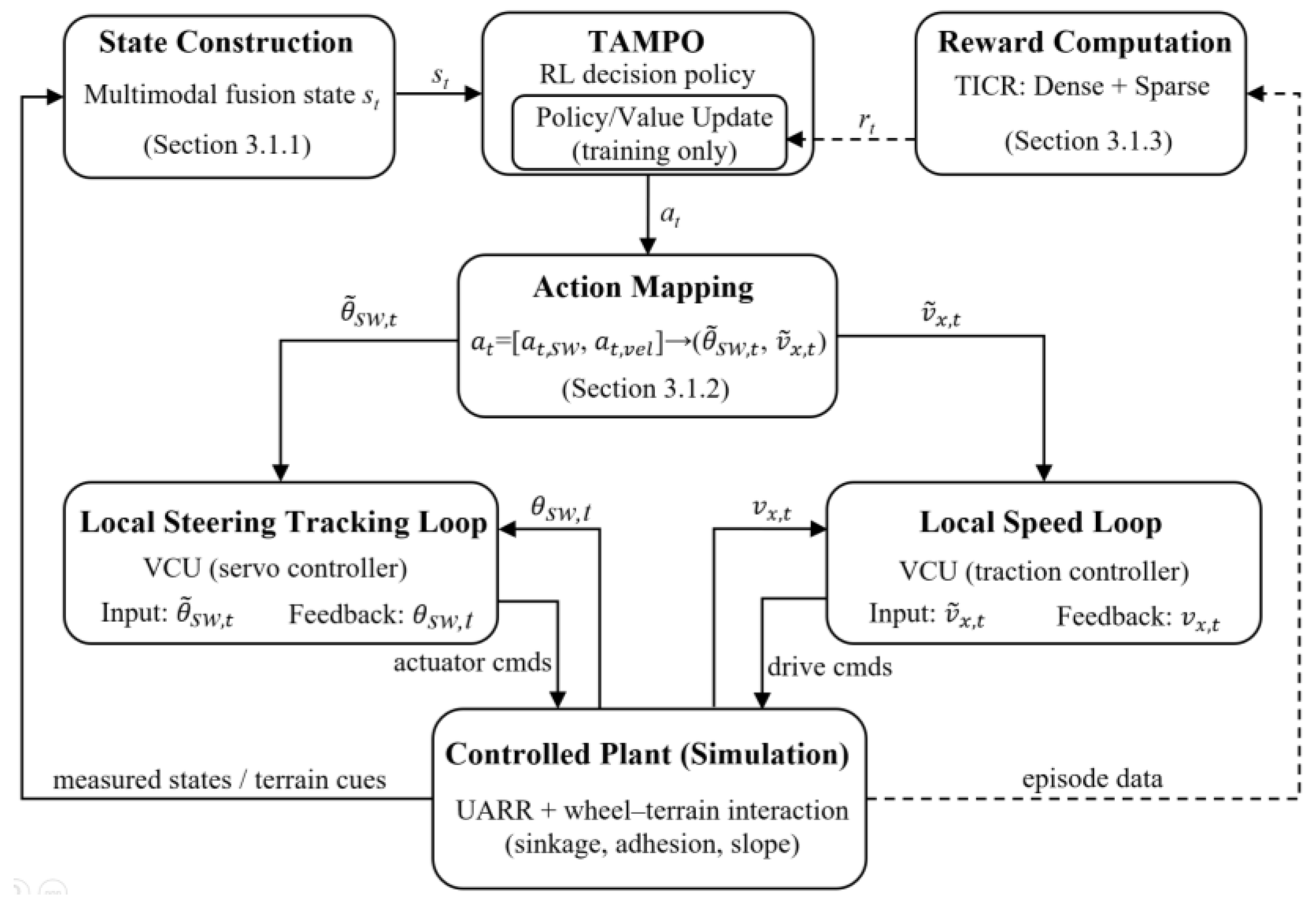
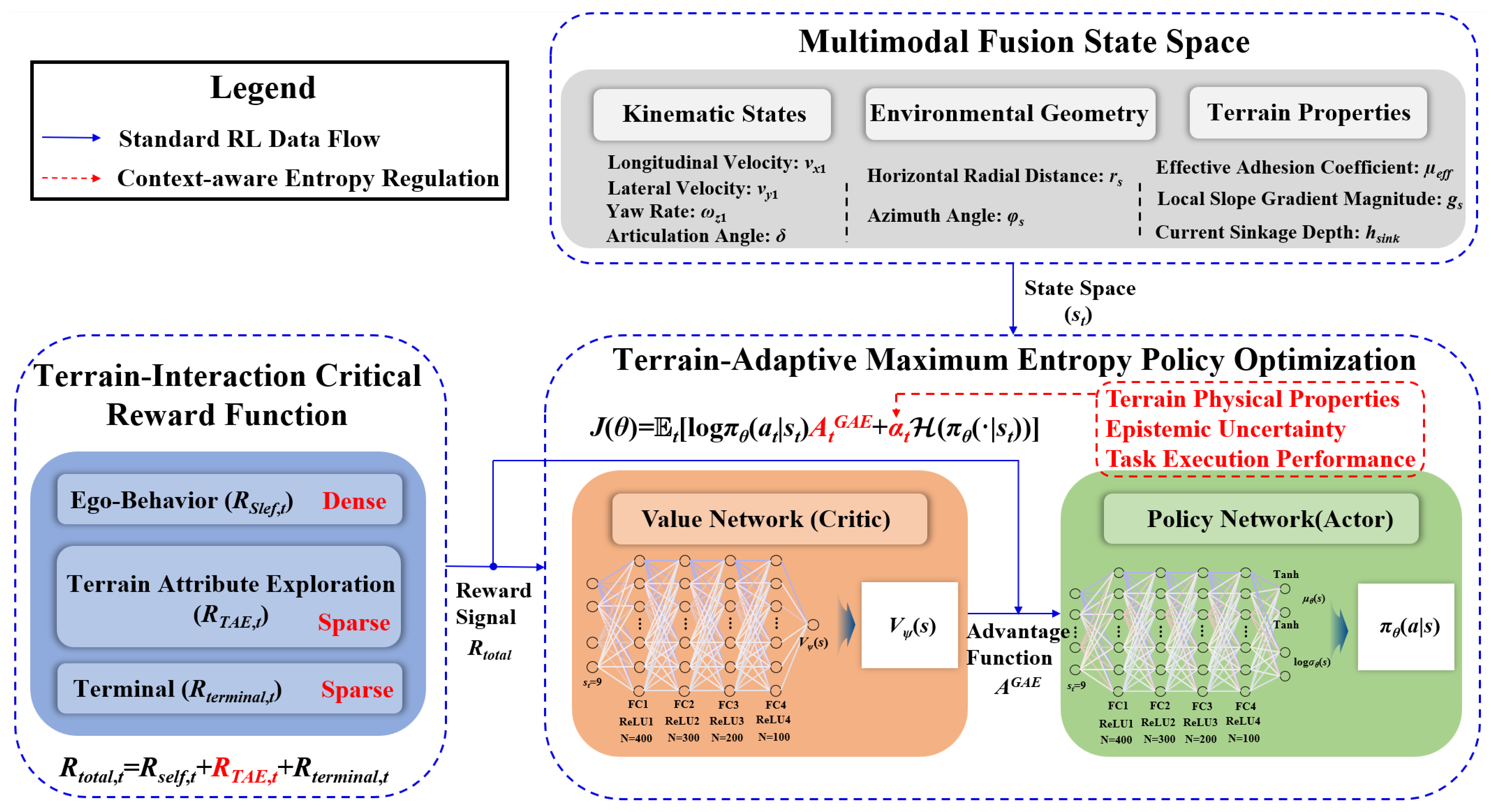
Although the proposed TAMPO is formulated as a reinforcement-learning policy over the MDP defined in Section 3.1.1, Section 3.1.2 and Section 3.1.3, its deployment follows a hierarchical closed-loop control architecture consistent with industrial vehicle control practice. As shown in Figure 12, TAMPO operates as a high-level decision policy that maps the multimodal fusion state s t to normalized actions a t = [ a t , s w , a t , v e l ] . These actions are deterministically converted, via the action mapping and command shaping described in Section 3.1.2, into filtered reference commands θ ~ s w , t v ~ x , t for steering and longitudinal motion. The references are tracked by standard low-level local control loops (e.g., VCU/servo and traction controllers), which generate actuator/drive commands to the controlled plant (the articulated roller dynamics coupled with wheel–terrain interaction). The resulting measured kinematic states and terrain cues close the loop by updating the next-step state construction, thereby explicitly capturing the plant–controller interaction that underlies the MDP transition dynamics.
During training, the rollout data generated by this closed-loop interaction are further used to compute the Terrain-Interaction Critical Reward (TICR) in Section 3.1.3, which serves exclusively for policy optimization; the reward computation is not part of the online execution pipeline. Figure 12 clarifies the system-level interfaces between the learned decision layer and the low-level tracking loops, while the internal learning mechanism and context-aware entropy regulation of TAMPO are elaborated in Section 3.2 and Figure 13.

3.2. TAMPO Framework

3.2.1. Maximum-Entropy Actor–Critic

To solve the MDP defined in Section 3.1, an actor–critic (AC) architecture is adopted as the algorithmic backbone [34,35]. The actor (policy network) generates actions in a continuous space, while the critic (value network) evaluates their performance and supplies low-variance value baselines, thereby improving sample efficiency and training stability [36,37].
To mitigate the heavy reliance of conventional AC on external exploration noise and to avoid premature convergence to suboptimal policies, the maximum-entropy reinforcement learning paradigm is further incorporated [38]. In this paradigm, a regularization term that encourages high policy entropy H ( π θ ( s t ) ) is added to the standard discounted return objective, trading off between maximizing cumulative return and maximizing policy diversity. The resulting objective is as follows:
J ( π θ ) = E τ ~ π θ t = 0 T γ t r t + α H ( π θ ( | s t ) ) .
Here, the temperature coefficient α 0 balances the relative importance of expected return against the degree of policy stochasticity.
Within the AC update, directly using cumulative returns U t tends to introduce high variance due to sampling uncertainty [39]. To alleviate this issue, the advantage function A ( s , a ) is used to guide policy updates, defined as the action-value minus the state value, see Equation (29):
A π ( s , a ) = Q π ( s , a ) V π ( s ) .
This quantity measures the improvement achieved by taking action a at state s relative to the current policy’s average behavior V π ( s ) . For accurate and stable advantage estimation in practice, generalized advantage estimation (GAE) is employed [40,41]. GAE exponentially weights multi-step temporal-difference (TD) errors to balance bias and variance, as shown in Equation (30):
A t G A E = k = 0 ( γ λ ) k δ t + k , δ t + k = r t + k + γ V π ( s t + k + 1 ) V π ( s t + k ) .
The parameter λ [ 0 ,   1 ] is the decay factor that controls this trade-off.

3.2.2. Limitation of Entropy Regularization with a Global Target

Although soft actor–critic (SAC) treats α as a learnable parameter and tunes it by minimizing an auxiliary loss toward a global target entropy, see Equation (31):
L ( α ) = E a ~ π θ ( | s ) α ( log π θ ( a | s ) H t a r g e t ) .
This automatic adjustment is task-agnostic and oblivious to the real-time physical context. For the coupled-terrain traversal studied here, a single global (or task-independent) entropy target is suboptimal. The agent’s exploration intensity should adapt online to the current physical conditions.
In standard SAC, the temperature-tuning mechanism cannot satisfy this need for context-dependent modulation driven by physical information. If key terrain factors—such as terrain difficulty, feasible progress, and value uncertainty—can be fused into a data-driven schedule for α , the desired behavior of “explore when necessary, exploit for efficient return” can be realized, thereby overcoming the core limitation of the conventional approach.

3.2.3. Target Core Mechanisms and Update Flow

This section proposes a context-aware TAMPO algorithm. By leveraging three-fold environmental feedback to adjust the entropy coefficient online, the method achieves dynamic adaptation for the mud-pit escape task. Figure 13 outlines the proposed solution.
(1)
Context-aware adaptive entropy regularization:
  • Terrain physical properties. The instantaneous difficulty index D t and its exponentially smoothed result D t * are used to quantify traversal difficulty; both are defined in (15) and (17).
  • Task-execution efficacy. A progress-based moving average is constructed as the advancement indicator η t ; its update is given in Equation (32):
    η t = ρ η η t 1 + ( 1 ρ η ) max ( 0 , r p r o g r e s s , t ) .
  • Epistemic uncertainty. The normalized sample standard deviation of the value network output, σ V , t n o r , is adopted as a proxy; the definition is given in Equation (33), and the online maintenance of its upper bound σ V m a x in Equation (34):
σ V , t n o r = σ V , t σ V max ,
σ V max max ( σ V max , σ V , t ) .
Combining the three feedback signals above, the entropy coefficient is scheduled online as α t ; the rule is given in Equation (35) (with α m i n as the lower bound, α 0 as the initial value, β H as the time-decay rate, and λ D , λ η , λ V 0 as the weights for “difficulty-progress-uncertainty”).
α t = max α min , α 0 e β H t ( 1 + λ D D t * λ η η t + λ V σ V , t n o r )
It is worth noting that TICR does not directly dictate the exploration strength. Instead, the reward influences exploration only indirectly through its effect on the return and the advantage estimate A t G A E , which, in turn, affects the context variables used in α t . In the proposed mechanism, the policy temperature is an explicit state-dependent function of the terrain’s physical difficulty D t * , a progress-based convergence indicator η t derived from the accumulated total reward and the normalized value-function uncertainty σ V , t n o r By jointly encoding “terrain difficulty–learning progress–epistemic uncertainty’’ in the entropy coefficient, the exploration–exploitation balance is adapted according to physically interpretable task context, rather than being driven by a single generic signal such as state entropy or value variance.
(2)
Value and advantage estimation based on GAE.
The critic V ψ approximates the state-value function. The TD target uses a Polyak-averaged target network V ψ t g t ; the TD error is defined in Equation (36):
δ t = R t o t a l , t + γ V ψ t g t ( s t + 1 ) V ψ ( s t ) .
The critic loss is the MSE of the TD error, see Equation (37), and parameters are updated by gradient descent, see Equation (38):
L c r i t i c ( ψ ) = E t δ t 2 ,
ψ ψ η ψ ψ L c r i t i c ( ψ ) .
The target network is updated via Polyak averaging, see Equation (39):
ψ t g t ( 1 τ ) ψ t g t + τ ψ .
GAE is adopted to provide stable, low-variance advantage targets for the actor; A t G A E is given in Equation (40) (with λ [ 0 ,   1 ] ):
A t G A E = k = 0 ( γ λ ) k δ t + k
(3)
Entropy-regularized policy update.
The actor maps a state s to a diagonal-Gaussian policy and samples an action a ; the parameterization is given in Equation (41) (with a minimum std σ m i n to ensure sufficient exploration):
π θ ( a | s ) = N μ θ ( s ) , d i a g ( σ θ ( s ) 2 ) ,   σ θ ( s ) σ min
The entropy-regularized objective maximizes the sum of the log-probability term weighted by the advantage and the policy entropy weighted by α t ; the objective is given in Equation (42):
J ( θ ) = E t log π θ ( a t | s t ) A t G A E + α t H ( π θ ( | s t ) ) .
The corresponding policy gradient is given in (43):
θ J ( θ ) = E t θ log π θ ( a t | s t ) A t G A E + α t θ H ( π θ ( | s t ) ) .

3.2.4. Neural-Network Architecture and Hyperparameter Settings

Implementation of TAMPO relies on two parallel function approximators, a policy network (Actor, π θ ) and a state-value network (Critic, V ψ ), which approximate the optimal policy and the value function, respectively. Network topology, depth, activations, and optimizer settings were found to have decisive impact on sampling efficiency, training stability, and convergence under the on-policy paradigm [42]. In all experiments, Adam was adopted to update both networks.
(1)
Policy network (Actor)
The actor maps the input state vector s t to a Gaussian policy π θ ( a s ) . A multi-layer perceptron (MLP) [43] is employed with four fully connected hidden layers of sizes 400-300-200-100 (progressively decreasing to encourage hierarchical feature compression and abstraction). ReLU activations are used in all hidden layers [44]. The output head is factorized into two parallel branches to parameterize a bivariate Gaussian:
  • Mean head. A 2-D output provides the means for steering and longitudinal-velocity actions. A tanh activation is applied to normalize outputs to [ 1 ,   1 ] , matching the normalized action space.
  • Log-standard-deviation head. A 2-D output provides l o g σ θ ( s t ) . The standard deviation is obtained by exponentiation, guaranteeing positivity and numerical stability. This design keeps the sampling operation differentiable and supports efficient policy-gradient computation.
During interaction, the executed action a t is sampled from N ( μ θ ( s t ) , d i a g ( σ θ ( s t ) 2 ) ) , satisfying the entropy-regularized framework’s requirement of intrinsic stochasticity.
(2)
Value network (Critic)
The critic approximates the state-value function V ( s ) . It shares the same MLP topology and normalized 9-D state input as the actor. The output layer contains a single linear unit that regresses the scalar estimate V ψ ( s t ) .
To mitigate instability caused by bootstrapping, a target value network V ψ t g t is maintained and soft-updated via Polyak averaging with coefficient τ [45]. The hyperparameter settings used for training TAMPO are summarized in Table 5.

4. Simulation Training and Generalization Evaluation

4.1. Experimental Setup

To comprehensively assess the agent’s learning and generalization in mud-pit environments, the 3-D parameter space Ω (864 distinct scenarios) was partitioned into a training set and an in-domain test set, and an additional extrapolation test set beyond Ω was constructed, yielding three mutually disjoint datasets:
(1)
Training set Ω train :
A total of 768 scenarios covering all parameter combinations except b m = 3   m . This set is used to train all algorithms under evaluation.
(2)
Interpolation test set Ω test interp :
A total of 96 scenarios constructed with the configuration unseen in training (fixed b m = 3   m ). This set evaluates in-domain generalization.
(3)
Extrapolation test set Ω test extrap :
A total of 90 scenarios generated by selecting parameter values outside the training grid and by reseeding the Perlin noise to emulate different local heterogeneity. The subsets are as follows:
  • Adhesion coefficient set: S μ extrap = { 0.37 ,   0.52 ,   0.68 } ;
  • Depth set: S d extrap = { 0.10 ,   0.20 ,   0.30 ,   0.42 ,   0.50 ,   0.60 ,   0.70 ,   0.82 ,   0.90 ,   1.00 }   m ;
  • Rim-size set: S b m extrap = { 1.8 ,   3.3 ,   4.8 }   m .
During the entire experimental pipeline, only Ω train was accessed for training. At the beginning of each episode, one scenario was sampled uniformly at random from Ω train to ensure exposure to mixed-difficulty terrains. The two test sets were used for periodic offline evaluation; no information from them was ever leaked into training, guaranteeing independence and fairness.
To benchmark the proposed TAMPO method, three widely used deep RL baselines representing different technical routes were adopted: PPO [41], SAC [15], and DDPG [46]. All algorithms used matched network architectures and optimizers, with their task-specific hyperparameters finely tuned to ensure a fair comparison. The specific settings for these baseline algorithms are detailed in Appendix A.
For multi-faceted quantitative evaluation, three core metrics were defined:
(1)
Success Rate (S.R.): The proportion of episodes in which the agent successfully escapes the pit. This serves as the primary metric of strategic effectiveness.
(2)
Average Escape Time (A.E.T.): The mean time from episode start to successful escape, computed only over successful episodes, reflecting policy efficiency.
(3)
Average Cumulative Reward (A.C.R.): The mean cumulative return over all episodes (successful or failed) on the test sets, reflecting the overall quality of the policy.

4.2. Training-Process Comparison

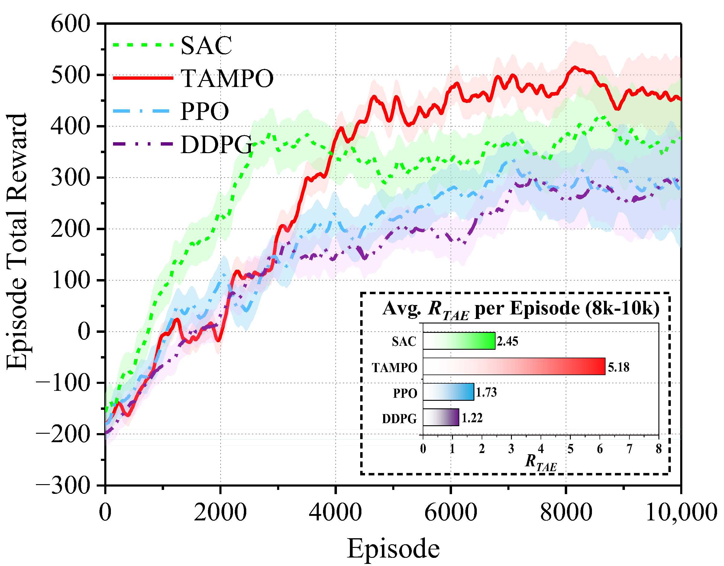
The proposed TAMPO algorithm and three baselines were analyzed in-depth on the training set Ω train . Figure 14 presents the evolution of the average cumulative reward over 10,000 training episodes, with the inset showing the average terrain-attribute exploration reward R - T A E per episode during the late training phase (episodes 8 k–10 k).
It can be observed that the four algorithms exhibit distinct learning characteristics. SAC, as an off-policy method, learns fastest in the early stage and reaches its first peak around episode 2900. However, a pronounced performance plateau follows, and the reward curve oscillates and even drifts down slightly, reflecting that its entropy auto-tuning—agnostic to terrain difficulty—struggles to sustain effective exploration under highly heterogeneous mud-pit conditions. PPO, as an on-policy method, shows the smoothest learning trajectory but converges to a lower final return, limited by its relatively conservative exploration mechanism. DDPG performs the worst overall; its deterministic exploration fails to cope with the task’s complex challenges and ends at the lowest level.
In contrast, the proposed TAMPO shows rapid improvement after about 2000 episodes of initial exploration, when the context-aware entropy adaptation starts to take effect. The learning efficiency is thereby enhanced, and the method exhibits the steepest mid-training slope among all algorithms, with convergence reached after about 6500 episodes. This is evidence that TAMPO’s dynamic adjustment of exploration strength mitigates the learning plateau seen in other methods and enables discovery of better strategy improvements.
Moreover, the inset indicates that TAMPO achieves the highest late-phase average R - T A E (≈5.18), clearly surpassing the baselines. This suggests that TAMPO maintains a high overall return while persistently discovering and exploiting favorable high-adhesion patches, thereby validating the effectiveness of the proposed terrain-adaptive exploration mechanism.

4.3. Quantitative Assessment of Generalization Performance

To systematically evaluate the final performance of each algorithm after training convergence and its generalization capability in unseen environments, this section conducts a comprehensive quantitative evaluation. The final trained models of TAMPO and three baseline algorithms are assessed on two independent test sets: the interpolation test set Ω t e s t interp and the extrapolation test set Ω t e s t extrap . The comprehensive performance of each algorithm on these two test sets is measured by success rate (S.R.), Average Escape Time (A.E.T.), and average cumulative reward (A.C.R.). The statistical results are presented in Table 6.
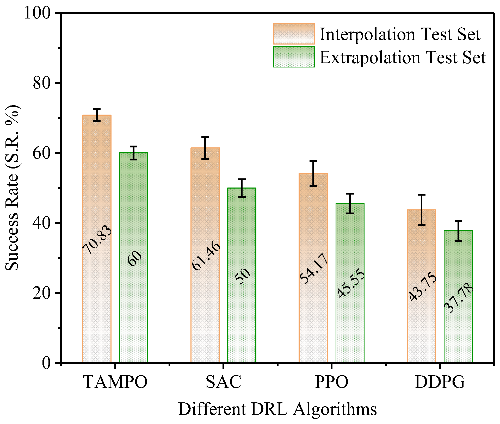
The quantitative evaluation results (Table 6) demonstrate that TAMPO exhibits a significant advantage in absolute performance. Its success rate on the interpolation test set reached 70.83%, considerably higher than all baseline algorithms. On the extrapolation test set, which features a broader distribution of mud-pit scenarios and is designed to assess out-of-distribution generalization, TAMPO was the only algorithm to maintain a 60% success rate. In contrast, the performance of all other algorithms dropped below 50%, highlighting the efficiency and robustness of the TAMPO policy.
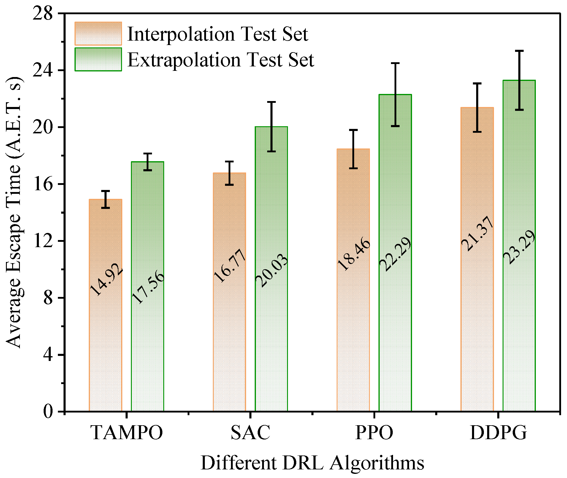
As shown in Figure 15, TAMPO’s success rate dropped by 10.83%, which is larger than the 5.97% drop of the worst-performing DDPG. However, this mainly reflects TAMPO’s robustness given its much higher baseline performance. The small decrease in DDPG is a typical “floor effect” caused by its inefficient policy: the low initial performance leaves little room for further degradation. For generalization, the key criterion is the absolute performance that can be maintained in more difficult, unseen environments, under which TAMPO exhibits the strongest generalization capability. Regarding escape efficiency (Figure 16), TAMPO also achieves the lowest Average Escape Time (A.E.T.) on both test sets. Considering these two metrics together, the policy learned by TAMPO attains both the highest success rate and the best time efficiency on the complex mud-pit escape task.
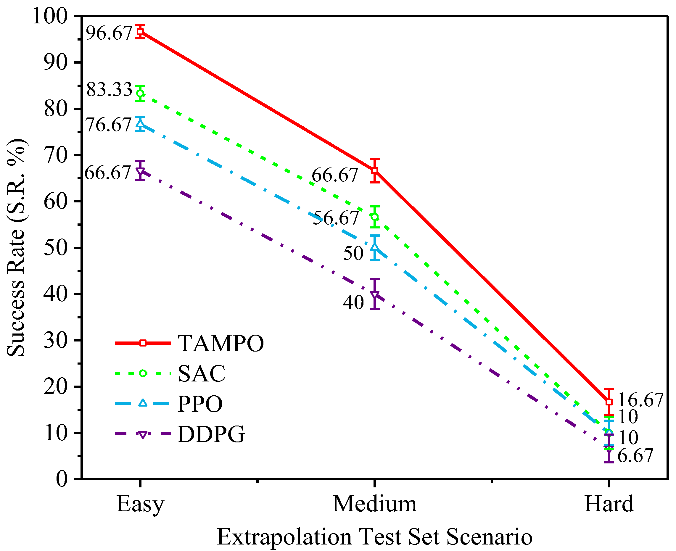
To further examine the robustness of each algorithm across different difficulty levels, a difficulty function is introduced in (44). The extrapolation test set, which has the broadest scenario coverage, is partitioned into three subsets—Easy, Medium, and Hard—according to this difficulty measure, and the performance of each algorithm is evaluated separately on each subset:
D s c e n e ( μ , d , b m ) = w μ μ max μ b a s e μ max μ min + w d d D d r u m + w μ b max b m b max b min ,
where μ b a s e S μ extrap , d S d extrap , and bm S b m extrap . The weight vector ( ω μ , ω d , ω b m ) = (0.3, 0.5, 0.2) was determined through preliminary experimental optimization, normalizing the respective contributions of the adhesion coefficient, pit depth, and rim size.
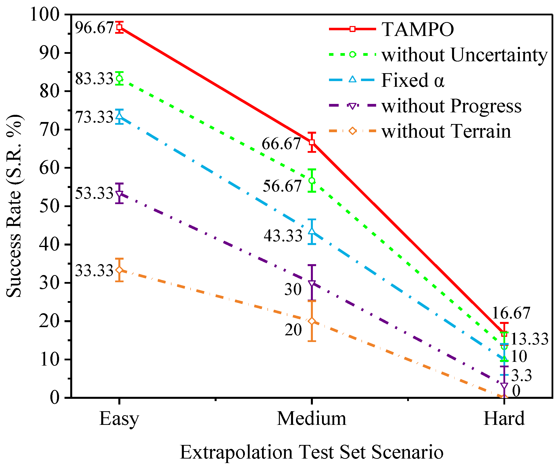
Figure 17 shows a performance breakdown of each algorithm across scenarios of varying difficulty within the extrapolation test set. The success rates of all algorithms decrease monotonically as scenario difficulty increases. At the ‘Hard’ level, however, all algorithms undergo a sharp performance degradation: the success rates of the sub-optimal SAC and PPO drop to 10.00%, whereas TAMPO maintains the highest success rate at 16.67%, indicating superior robustness. These results indicate that the advantage of TAMPO is most pronounced in highly difficult, strongly uncertain, unseen environments. Although its context-aware mechanism is not completely immune to severe challenges, it can still identify and execute effective policies to the greatest extent, thereby retaining the highest probability of task success even in scenarios where the baseline algorithms nearly fail.

4.4. TAMPO Algorithm Ablation Study

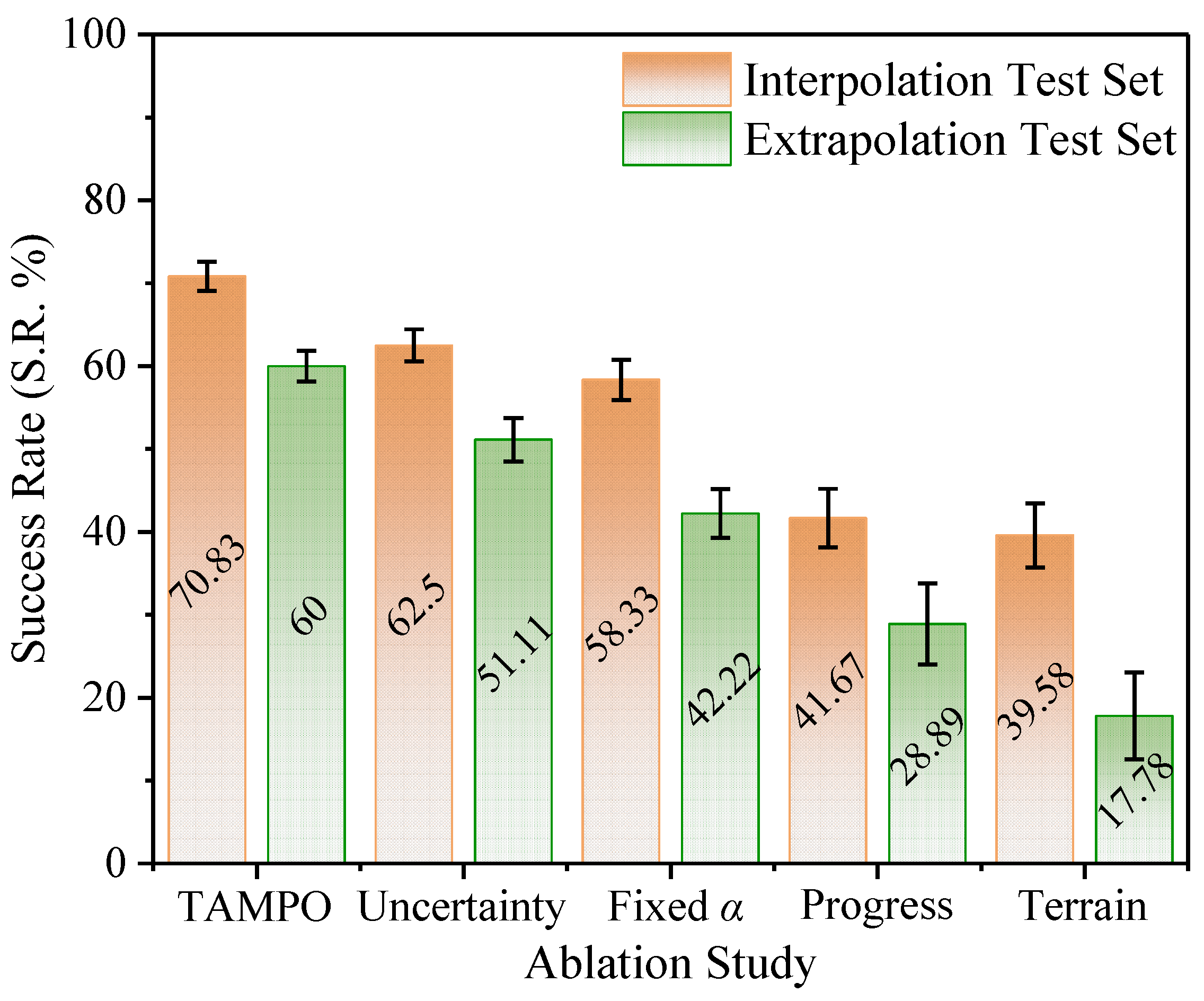
To assess the necessity and effectiveness of each core component in the proposed context-aware mechanism for adaptive entropy regularization, an ablation study is conducted on the TAMPO algorithm. Four ablated variants are obtained by removing specific functional modules from the full TAMPO algorithm. All variants are trained on the Ω train set and evaluated on the interpolation test set Ω test interp and the extrapolation test set Ω test extrap . The variants are as follows:
(1)
Removing the exploration term driven by value-network uncertainty σ V , t nor , with setting λ V = 0 ;
(2)
Removing the progress-dependent feedback term η t , with setting λ η = 0 ;
(3)
Removing the terrain difficulty feedback term D t * , with setting λ D = 0 ;
(4)
Removing the adaptive entropy-coefficient mechanism and replacing it with a finely tuned fixed constant.
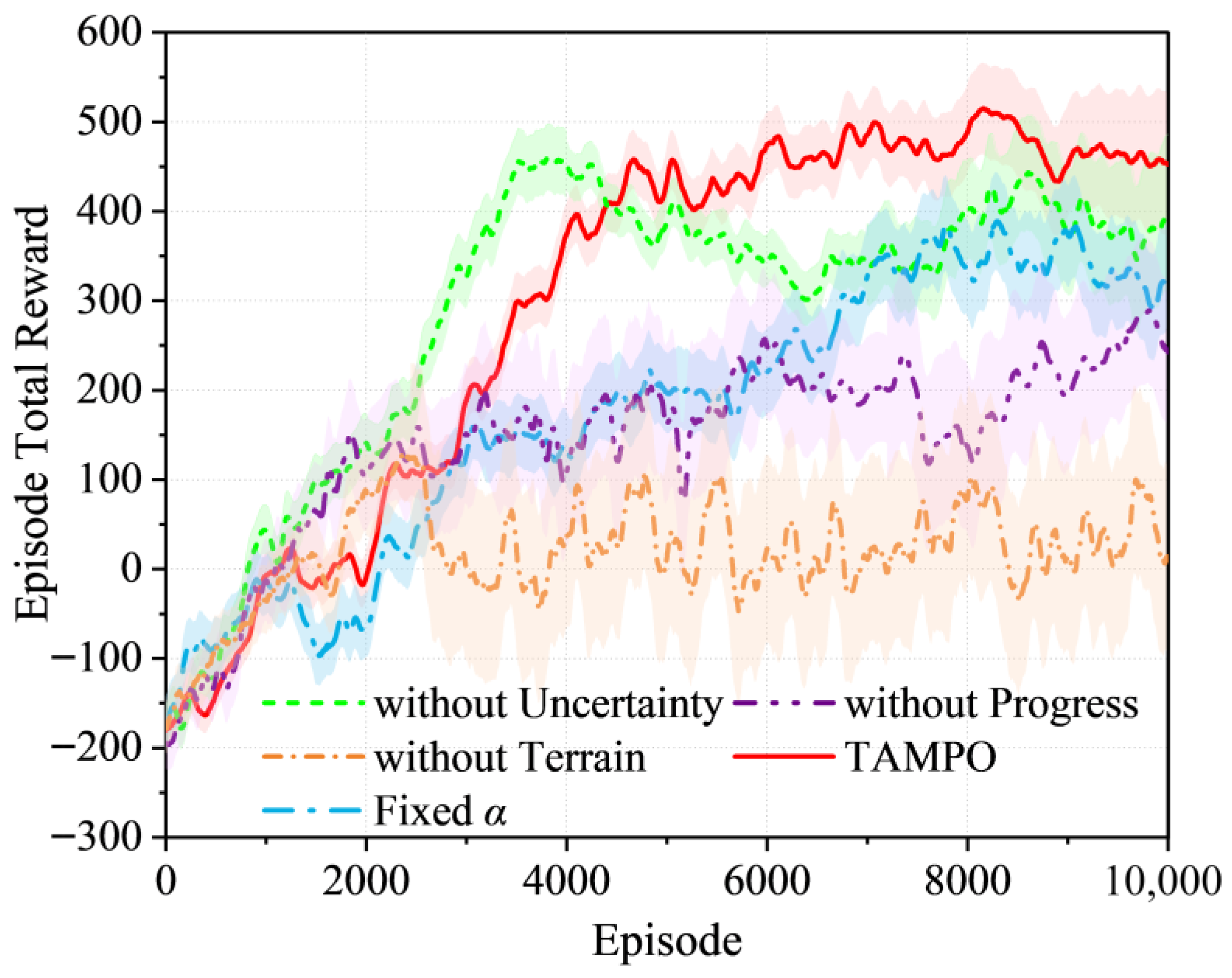
Figure 18 displays the average cumulative reward curves of the full TAMPO and its four ablation variants during training, highlighting the influence of each component on the learning dynamics.
The variant without the value-uncertainty term (green line) loses the exploration drive from epistemic uncertainty and behaves more greedily, quickly exploiting the policy learned in simple early-stage scenarios. This short-sighted behavior leads to insufficient exploration and poor policy generalization: when a broader range of complex scenarios appears later in training, the fragility of the policy is exposed, and its performance drops sharply from its peak, confirming the necessity of uncertainty-driven exploration for learning robust policies. The fixed-entropy-coefficient variant (blue line), which cannot dynamically balance exploration and exploitation, exhibits a smooth and stable learning curve but ultimately converges to a sub-optimal level. The variant without the progress-feedback term (purple line) shows a severe defect in its exploration–exploitation trade-off. Due to the loss of the negative feedback from η t , the algorithm converges prematurely to a low-performance level once a sub-optimal policy is found and lacks the ability to reincrease exploration. The variant without the terrain-difficulty term (orange line) performs the worst. Its learning curve displays a “pseudo-prosperity” pattern: during roughly the first 2400 episodes, the curve rises rapidly because difficult scenarios are rarely encountered; once challenging terrains appear frequently, performance collapses and enters a long-lasting low-level oscillation (between 0 and 100 A.C.R.). Without this core physical cue, the agent cannot associate escape failures with specific terrain challenges. The advanced policy learned in simple scenarios fails immediately on difficult terrain, leading to an irrecoverable low-performance oscillation.
To quantitatively assess the impact of each component on final policy performance and generalization, Figure 19 reports the final success rates of all variants on the interpolation and extrapolation test sets. Figure 18 clearly shows that removing any single component from the context-aware mechanism causes a marked degradation in both test sets. The full TAMPO algorithm achieves the strongest generalization, with its success rate decreasing by only 10.83%, whereas the variant without terrain awareness suffers the largest drop at 21.80%. These results indicate that TAMPO’s context-aware adaptive mechanism operates as an integrated whole: it not only improves the absolute performance of the policy, but each component is also essential for maintaining generalization capability and robustness in unseen environments.
To further clarify the contribution of each component to robustness at a finer level, Figure 20 compares the performance of the variants across difficulty levels in the extrapolation test set. The Figure shows that although all algorithms achieve relatively high success rates in easy scenarios, their intrinsic weaknesses are greatly amplified as difficulty increases, leading to pronounced performance divergence. The full TAMPO algorithm, while also experiencing a substantial drop, still maintains the highest success rate of 16.67%, demonstrating the strongest performance resilience. By contrast, the variant without the progress-feedback term almost collapses, with a success rate of only 3.3%, and the variant without terrain awareness fails completely (0%), underscoring the decisive role of the terrain-awareness component in the context-aware mechanism.
Overall, the policies learned with TICR still display diverse and physically meaningful escape behaviors, such as actively searching for high-adhesion zones before attempting to climb out, indicating that the reward design does not over-constrain the solution space. The ablation results further show that performance degradation is mainly caused by removing key contextual feedback in the entropy schedule, rather than by minor variations in reward magnitudes. A more exhaustive sensitivity analysis of individual reward components and their weightings will be pursued in future work to provide an even finer-grained quantification of their contributions to learning and generalization.

4.5. Analysis of Typical Escape Scenarios

To gain deeper insight into the decision-making behaviors of the algorithms under specific challenges and to systematically evaluate their macroscopic generalization over the entire extrapolation test set, this section presents both a microscopic case analysis and a macroscopic performance evaluation.

4.5.1. Micro-Behavioral Analysis of Typical Scenarios

To isolate the effects of different difficulty factors, the pit opening was fixed at b m = 3.3   m during scenario selection. By combining different baseline adhesion coefficients and pit depths, three typical scenarios of increasing difficulty were constructed to analyze the behaviors of TAMPO and the baseline algorithms.
(1)
Easy Scenario ( μ b a s e = 0.68 , d = 0.5   m , b m = 3.3   m )
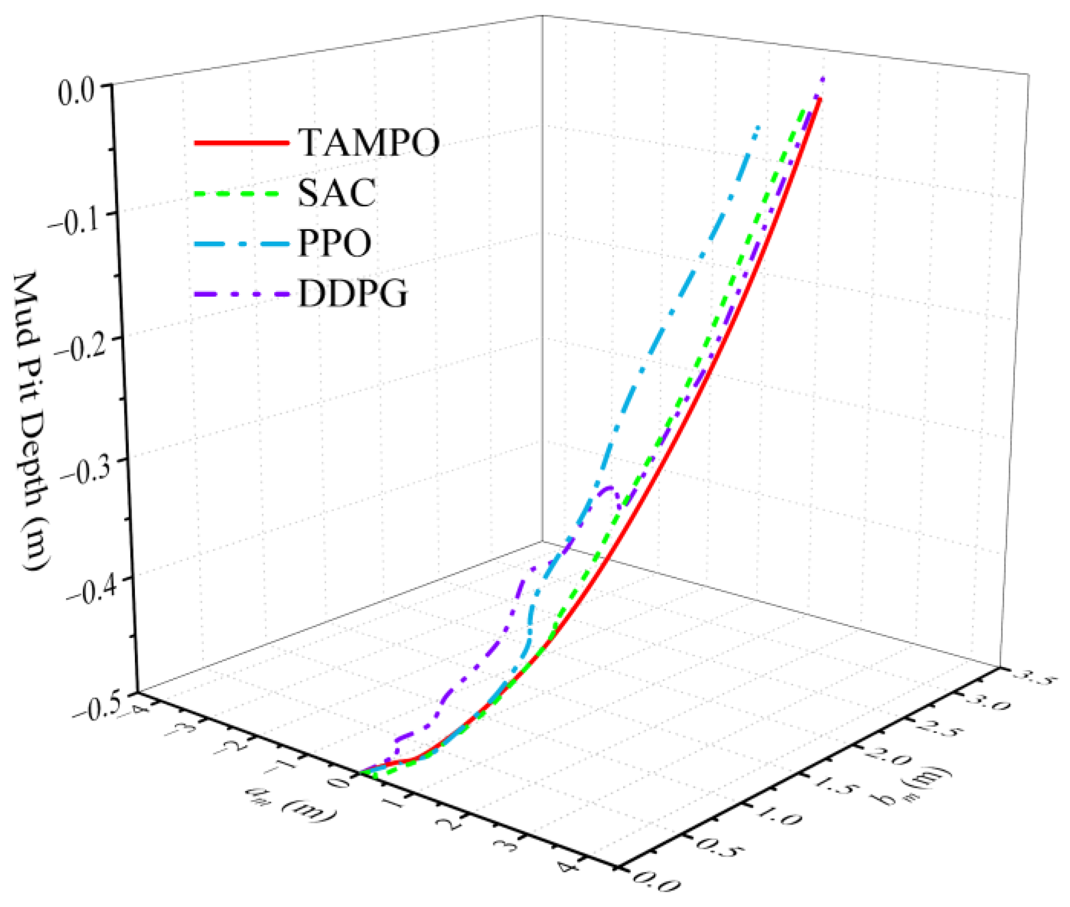
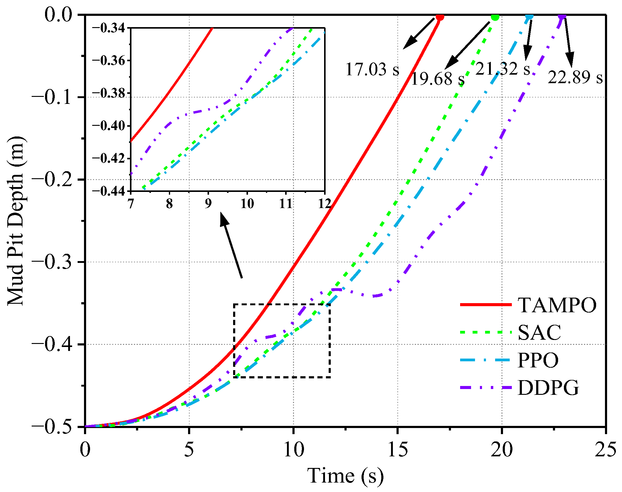
This scenario provides favorable conditions with a high adhesion coefficient and a shallow pit. All algorithms succeed within the maximum episode duration, but their decision efficiency and path quality differ markedly. Figure 21 shows the actual climbing trajectories of the agents: TAMPO follows the smoothest and most goal-directed escape path, whereas the baseline algorithms exhibit varying degrees of detours. As shown by the climb height–time curves in Figure 22, TAMPO completes the task first with a minimum time of 17.03 s, while DDPG is the slowest at 22.89 s, about 34% slower than TAMPO.
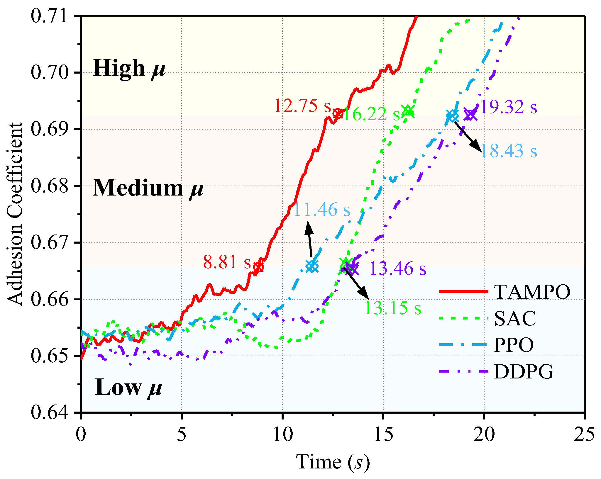
The adhesion–time curves in Figure 23 indicate that this efficiency gap stems from different terrain-interaction strategies. Benefiting from its context-aware mechanism, TAMPO enters the medium- and high-adhesion zones as early as 8.81 s and 12.75 s, respectively, clearly ahead of the baselines. This proactive search for and exploitation of favorable terrain directly reflects TAMPO’s intelligent exploration mechanism: once a high-return path is identified, the adaptive entropy coefficient α t decreases, suppressing unnecessary random exploration and enabling stable exploitation of the current optimal path.
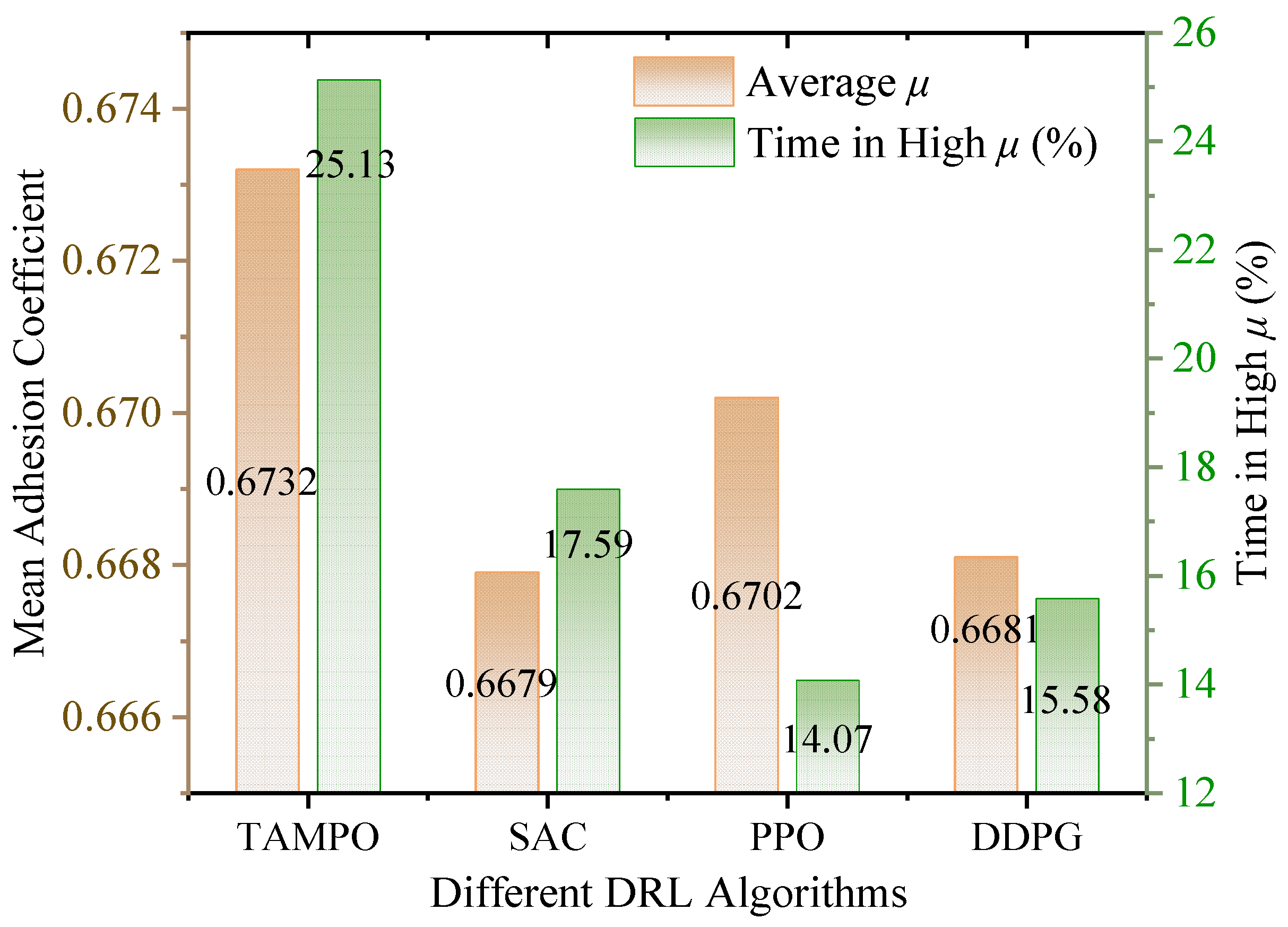
The statistics in Figure 24 further quantify this advantage: TAMPO achieves the highest mean adhesion coefficient (0.6732) and the largest proportion of time spent in the high-adhesion zone (25.13%). These results show that, even in simple scenarios, TAMPO’s adaptive exploration mechanism yields a decisive efficiency benefit.
(2)
Medium Scenario ( μ b a s e = 0.52 , d = 0.6   m , b m = 3.3   m )
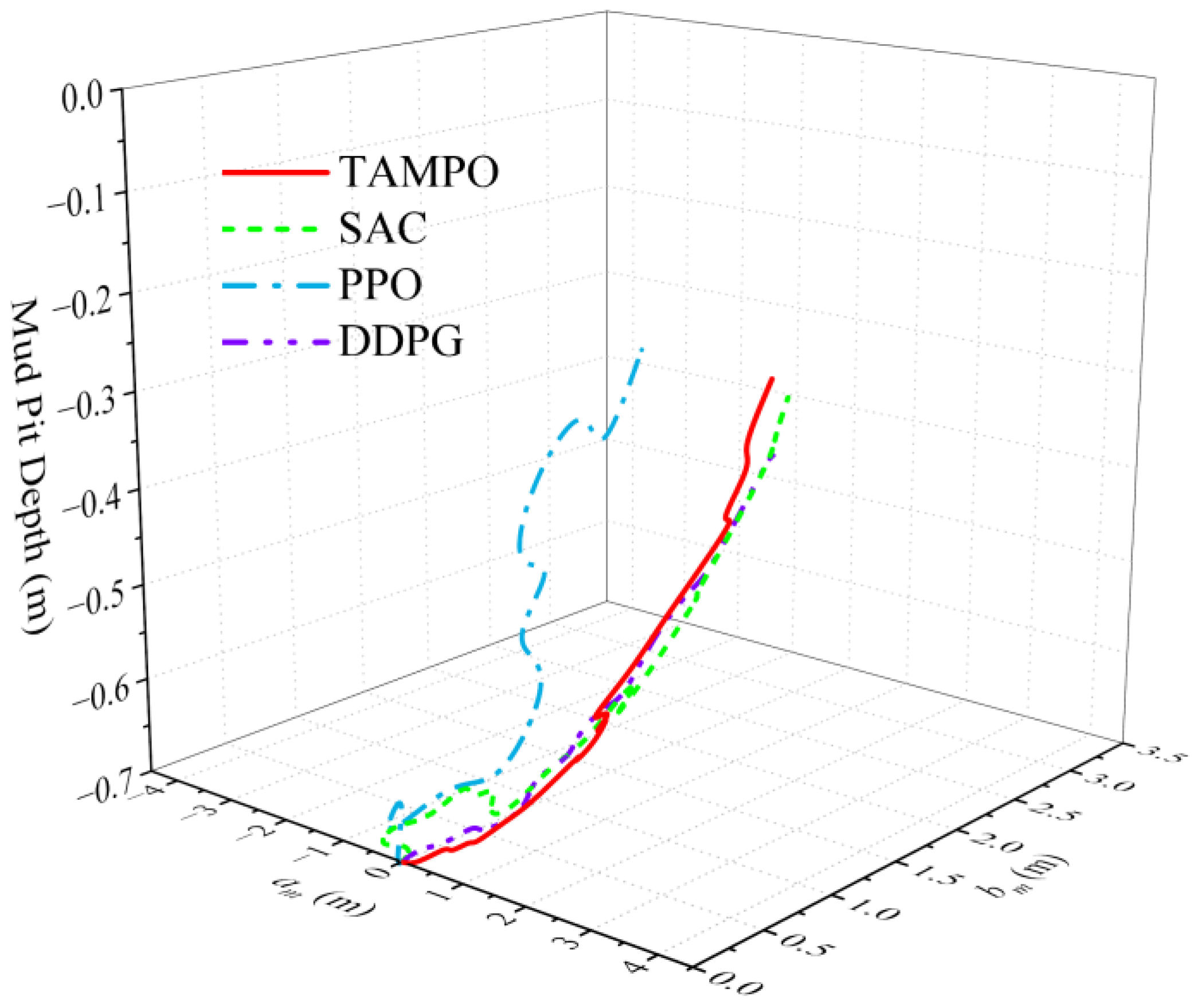
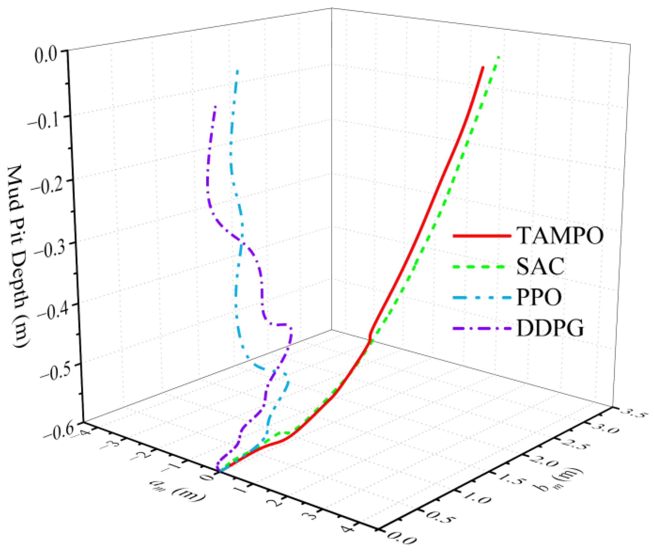
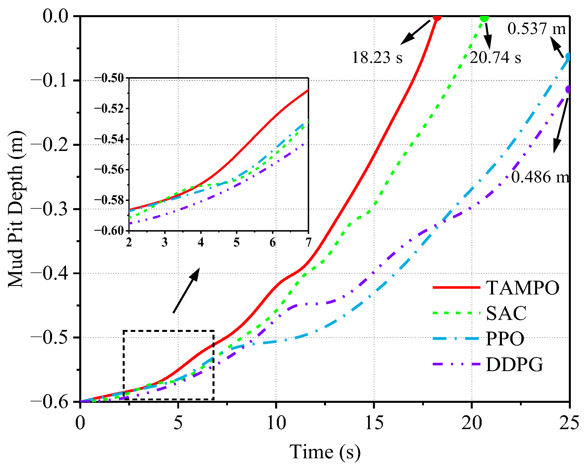
As environmental difficulty increases, the performance gaps between algorithms become more pronounced. In this medium-difficulty scenario, only TAMPO and SAC successfully escape, whereas PPO and DDPG fail. The climb-height–time curves in Figure 26 show that TAMPO succeeds in 18.23 s, while PPO and DDPG reach only 0.537 m and 0.486 m, respectively, within the episode time limit. The 3D trajectories in Figure 25 further reveal that the two failed baseline algorithms, PPO and DDPG, follow escape paths that differ markedly from those of the successful agents, leading them away from the feasible escape corridor.
Figure 25. Three-dimensional escape trajectories of different algorithms in medium scenario.
Machines 14 00079 g025
Figure 26. Climb height vs. time curves of different algorithms in medium scenario.
Machines 14 00079 g026
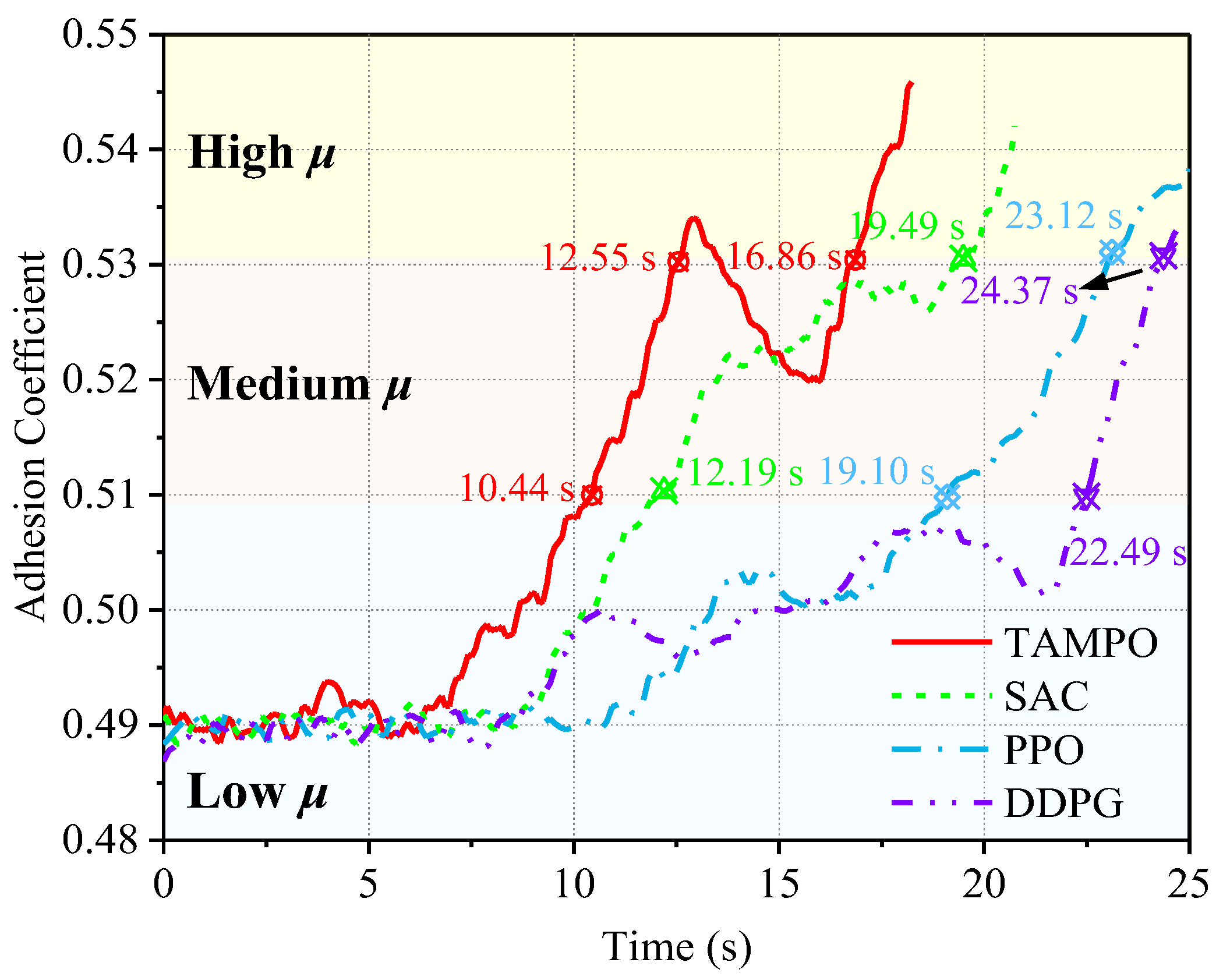
The adhesion–time curves in Figure 27 provide microscopic evidence for these trajectories. PPO and DDPG remain trapped in the low-adhesion zone for more than 75% of the episode, never discovering an effective path to the high-adhesion region. In contrast, TAMPO and SAC, benefiting from stronger exploration mechanisms, enter the medium-adhesion zone at 10.44 s and 12.19 s, respectively.
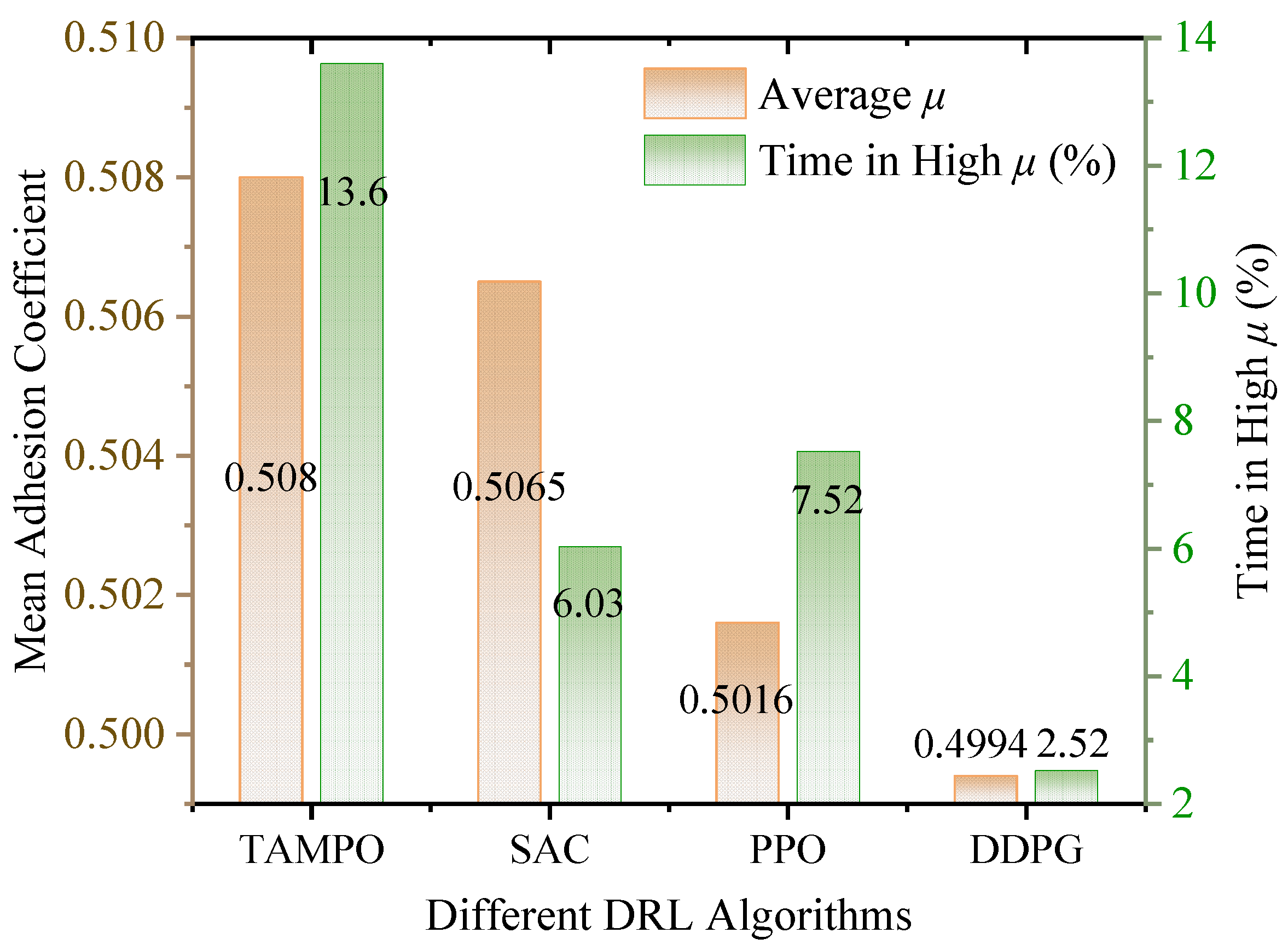
The statistics in Figure 28 further quantify this superiority. Although both TAMPO and SAC eventually escape, TAMPO spends 13.6% of the time in the high-adhesion zone—more than twice that of SAC (6.03%). This shows that TAMPO’s exploration is both effective and efficient, and confirms that its context-aware mechanism can rapidly reduce exploration entropy and then stably exploit the discovered optimal path.
(3)
Hard Scenario ( μ b a s e = 0.37 , d = 0.7   m , b m = 3.3   m )
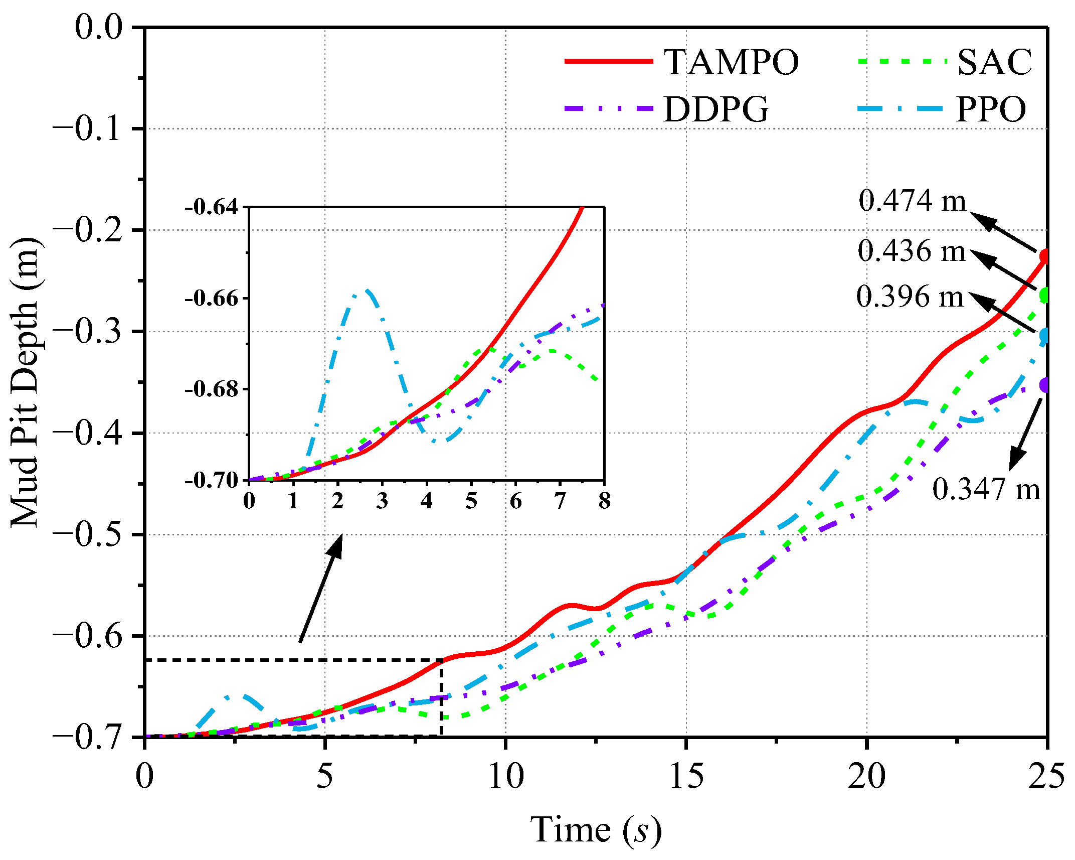
Under the harsh conditions of the hard scenario—low adhesion coefficient and a deep pit—all algorithms fail to complete the task, making this setting a stringent benchmark for performance resilience. As shown in Figure 30 (climb height–time), despite universal failure, TAMPO still attains the highest peak climb height of 0.474 m, clearly outperforming all baseline algorithms, whose limiting capabilities rank in the descending order of SAC, PPO, and DDPG. The 3D trajectories in Figure 29 further confirm that TAMPO maintains the strongest goal-directed trajectory among all algorithms.
Figure 29. Three-dimensional escape trajectories of different algorithms in hard scenario.
Machines 14 00079 g029
Figure 30. Climb height vs. time curves of different algorithms in hard scenario.
Machines 14 00079 g030
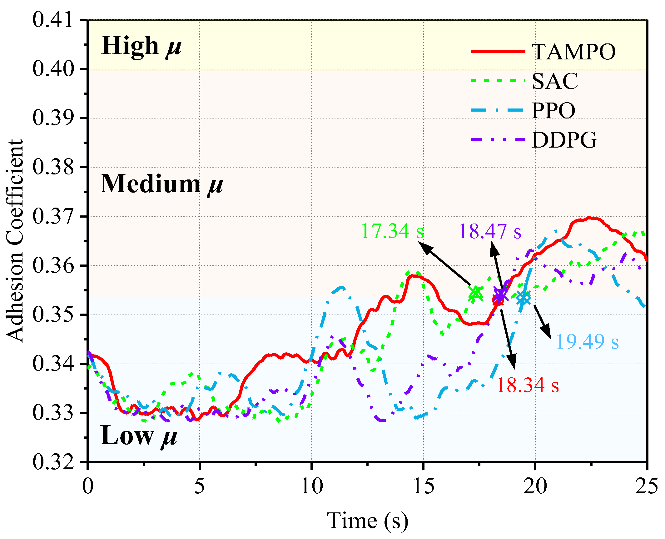
The adhesion–time curves in Figure 31 reveal the mechanism behind these differences. In this scenario, the ability to climb from the low-adhesion zone into the medium-adhesion zone determines the performance ceiling. SAC, driven by strong entropy-based exploration, is the first to enter and stabilize in the medium-adhesion region at 17.34 s. Although TAMPO reaches stable entry roughly 1 s later, its path quality is higher: once in this region, its adhesion coefficient remains almost entirely above that of SAC.
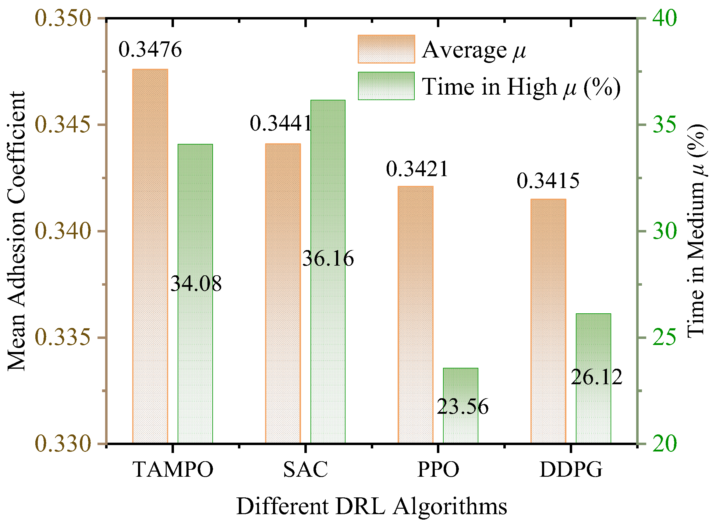
The final statistics in Figure 32 show that TAMPO’s dwell-time ratio in the medium-adhesion zone is 2.08% lower than that of SAC, yet it achieves the highest overall average adhesion coefficient. This indicates that TAMPO not only reaches feasible regions but also continues to search for more optimal trajectories. Such persistence in pursuing optimal decisions, even under extreme conditions, is the fundamental reason for its superior climbing performance.

4.5.2. Macroscopic Generalization Performance Evaluation

To systematically evaluate the generalization capability of the TAMPO algorithm across mud pits with different geometric morphologies, the 90 scenarios in the extrapolation test set are grouped into three categories according to the pit-opening short semi-axis set S b m extrap , and a macroscopic performance evaluation is conducted.
(1)
Narrow Pit Opening Scenarios ( b m = 1.8   m )
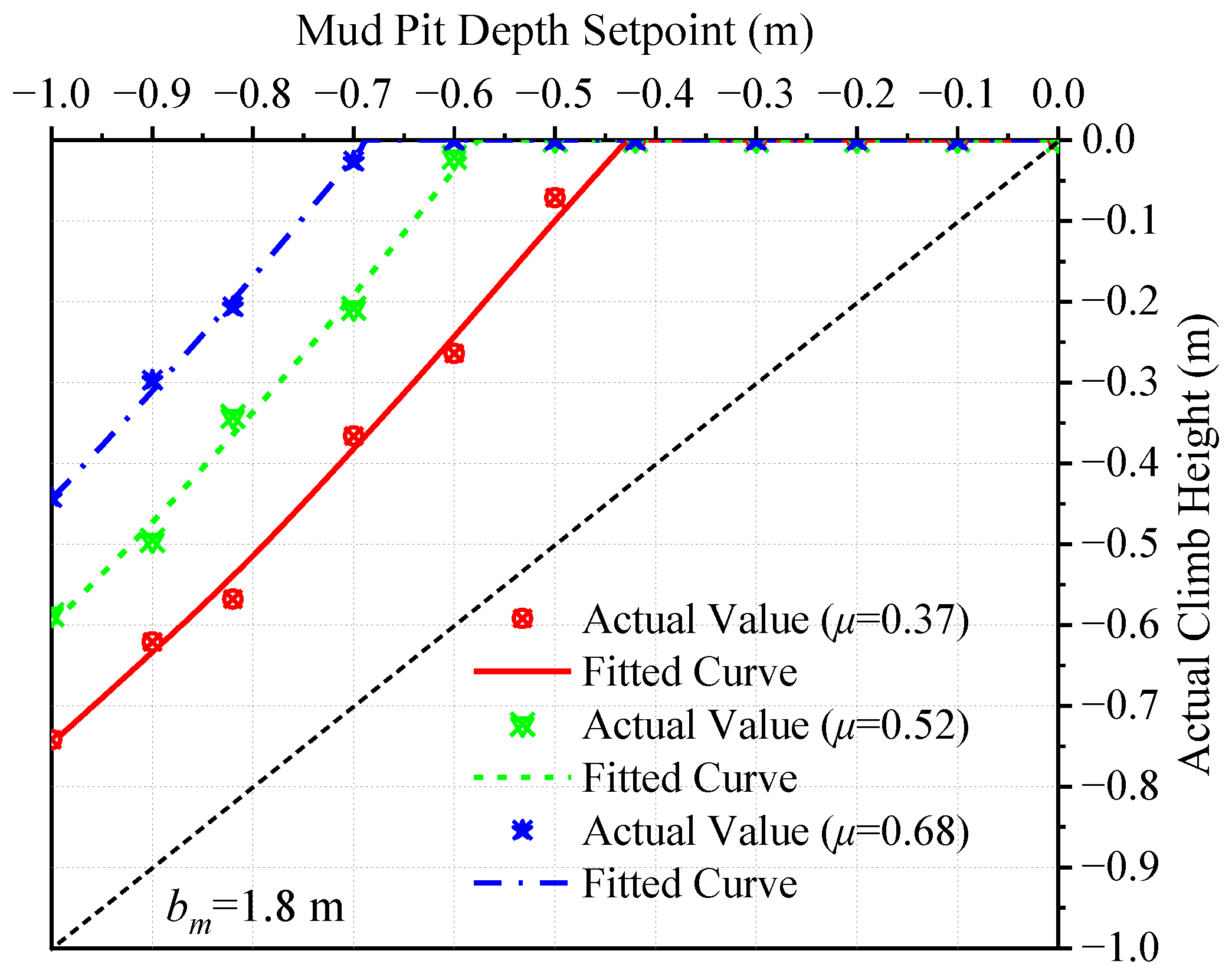
At the same depth, a narrow pit opening yields the steepest wall slope and thus the most stringent geometric constraint. Figure 33 shows the functional relationship between TAMPO’s escape capability limit, pit depth, and adhesion coefficient under this constraint, and Table 7 lists the corresponding peak climb heights.
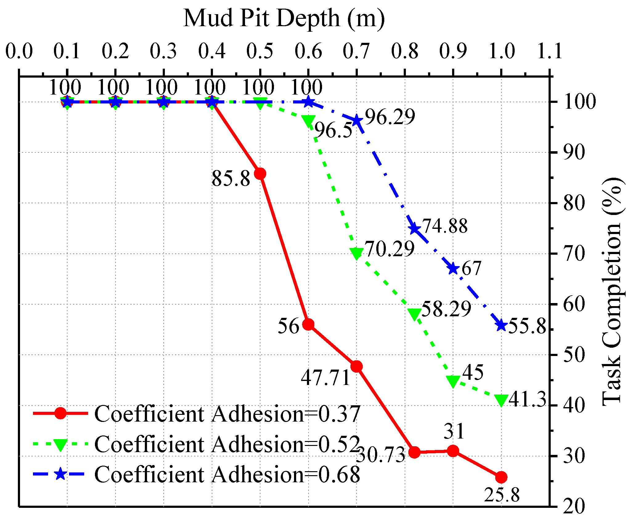
The results indicate that the agent’s performance is strongly suppressed under these harsh geometric conditions. Even under favorable high-adhesion conditions, the maximum depth for stable successful escape is only 0.6 m. When the adhesion coefficient decreases to 0.37, this capability boundary sharply contracts to 0.42 m. Figure 34 further quantifies this trend: all curves exhibit rapid performance decay, especially at low adhesion levels, and when the pit depth reaches 1.0 m, the task success rate drops to 25.8%. This shows that, in narrow, steep-walled mud pits, the agent’s escape capability is extremely sensitive to variations in adhesion coefficient and depth.
(2)
Medium Pit Opening Scenarios ( b m = 3.3   m )
When the short semi-axis is widened to b m = 3.3   m , the pit wall becomes gentler, and the agent’s escape performance improves markedly. As shown in Figure 35 and Table 8, TAMPO’s capability boundary extends to greater depths: under high-adhesion conditions, the maximum successful escape depth increases from 0.6 m in the narrow-opening case to 0.7 m, and even under low-adhesion conditions, the boundary still reaches 0.5 m.
In this medium-opening configuration, comparing the task-completion curves in Figure 34 and Figure 36 shows a consistent rightward shift and a delayed performance inflection point. This indicates that widening the opening effectively reduces task difficulty and raises the performance limit. For a fixed opening, the onset depth of performance degradation remains strongly tied to the baseline adhesion coefficient: as the adhesion level increases from low to high, the inflection point moves from 0.5 m to 0.7 m. Thus, higher adhesion effectively offsets the added difficulty induced by greater depth and broadens the range over which the agent can succeed stably.
(3)
Wide Pit Opening Scenarios ( b m = 4.8   m )
With the wide pit opening setting of b m = 4.8   m , the overall geometric difficulty of the task is minimized compared to the previous configurations. Consequently, TAMPO’s generalization capabilities and robustness are most fully exhibited. The performance depicted in Figure 37 and the corresponding data in Table 9 indicate that the agent’s capability boundary has been further pushed to its limit. Under high adhesion coefficient conditions, the successful escape depth reaches 0.82 m. It is noteworthy that even under severe conditions with a low adhesion coefficient, the capability boundary is maintained at 0.7 m, demonstrating exceptional robustness. As observed in the task completion curves in Figure 38, the performance degradation across all curves is the most gradual. This validates that within a gentle slope environment, the agent’s policy possesses stronger resilience against the other two adverse factors (depth and low adhesion).
The comparison across the three experimental groups reveals a consistent pattern: the geometric morphology of the mud pit, determined by the opening parameter b m , is the key physical factor modulating task difficulty. A narrower opening yields steeper walls, making the agent’s performance increasingly sensitive to deteriorating pit depth and adhesion. The core advantage of TAMPO lies in its ability to learn a generalizable policy with a deep understanding of terrain physical characteristics. It exhibits the highest performance resilience in the most challenging narrow-opening scenarios, while achieving the best task efficiency and policy stability in the easiest wide-opening scenarios. This behavior—spanning different geometric morphologies and degrading smoothly with increasing difficulty—demonstrates its strong practical value and robustness in high-difficulty, high-uncertainty, and unseen environments.

5. Conclusions

In this paper, a TAMPO algorithm is proposed to address the traversability challenges of UARRs operating on harsh terrains with coupled slipperiness and geometric irregularity. The proposed algorithm is systematically studied through multi-stage simulation validation:
  • A simulation platform based on a component-level physical network is constructed, comprising the road-roller system and parameterized mud-pit terrains. The vehicle model includes the drum, front frame, left and right rear wheels, rear frame, and hydraulic steering mechanism, with all subsystems built in accordance with the physical topology and assembly relationships of the real machine. The mud pit is modeled as a surface with elliptical contours and parabolic profiles. By combining the adhesion coefficient, pit depth, and the ellipse’s short semi-axis, parameterized scenarios are generated to form the training and test sets for the algorithms.
  • A TICR function is designed. By combining dense rewards that encode task progress with sparse rewards that encourage terrain exploration, this function provides informative guidance signals that enable the agent to learn efficient and intelligent escape policies.
  • The TAMPO algorithm is developed with a core context-aware adaptive entropy-regularization mechanism. By fusing, in real time, three types of information—terrain physical characteristics, task-execution efficacy, and model epistemic uncertainty—the mechanism dynamically adjusts policy entropy, thereby equipping the agent with the ability to intelligently balance exploration and exploitation in complex, heterogeneous environments.
  • TAMPO exhibits clear advantages in both escape effectiveness and efficiency. On the 90 most challenging scenarios in the extrapolation test set, TAMPO attains an average success rate (S.R.) of 60.00% with an Average Escape Time (A.E.T.) of only 17.56 s. Compared with PPO, SAC, and DDPG, the S.R. is improved by 10%, 14.45%, and 22.22%, respectively, while the A.E.T. is reduced by 2.47 s, 4.73 s, and 5.73 s, respectively. These results highlight the algorithm’s strong decision-making capability and generalization performance.

6. Future Work

In this study, the traversability performance of the TAMPO algorithm was validated on a UARR under fixed center-of-mass parameters. However, in the broader class of heavy-duty articulated machinery—such as articulated loaders and mining trucks—the mass, center-of-mass position, and moments of inertia can vary dramatically over the course of operation.
Future research may incorporate these time-varying inertial parameters as a key dimension of the state space and investigate reinforcement learning paradigms capable of identifying them online and embedding them into the decision-making process. Such extensions are expected to enable TAMPO-like frameworks to generalize across a wider range of articulated vehicle platforms.

Author Contributions

Conceptualization, W.Q. and H.X.; methodology, W.Q. and Q.X.; software, W.Q. and Q.X.; resources, W.Q. and Q.X.; validation, W.Q. and Q.X.; formal analysis, W.Q.; investigation, W.Q.; data curation, W.Q. and Q.X.; writing—original draft preparation, W.Q.; writing—review and editing, W.Q. and Q.X.; visualization, W.Q. and Q.X.; supervision, H.X.; project administration, W.Q.; funding acquisition, H.X.; All authors have read and agreed to the published version of the manuscript.

Funding

This work was supported by the National Key Research and Development Program of China under Grant 2022YFE0100100.

Data Availability Statement

The datasets presented in this article are not readily available because the simulation platform and datasets involve agent-related technologies currently under active research. Requests to access the datasets should be directed to the Advanced Power and Intelligent Vehicle Control Group at Tianjin University.

Acknowledgments

This research was initiated by the Advanced Power and Intelligent Vehicle Control Group at Tianjin University and was financially supported by the National Key R&D Program of China. The authors extend their sincere gratitude for this support.

Conflicts of Interest

The authors declare no conflicts of interest.

Abbreviations

The following abbreviations are used in this manuscript:
UARRUnmanned Articulated Road Roller
TAMPOTerrain-Adaptive Maximum-Entropy Policy Optimization
TICRTerrain-Interaction Critical Reward
S.R.Success rate
A.E.T.Average Escape Time
A.C.R.average cumulative reward
TCSTraction control systems
RLReinforcement learning
DAEDifferential-Algebraic Equation
MILModel-in-the-Loop
HILHardware-in-the-Loop
MDPMarkov decision process
ACActor–critic
TDTemporal-difference
SACSoft actor–critic
GAEGeneralized advantage estimation

Appendix A

Table A1. Hyperparameters for SAC neural-network training.
AlgorithmParameterValue
SACDiscount factor0.99
Actor learning rate0.0003
Critic learning rate0.001
Replay buffer size106
Batch size256
Target smoothing coefficient0.005
Initial temperature0.2
Entropy tuningTrue (Auto-learned)
Target entropydim(A) = −2
Table A2. Hyperparameters for PPO neural-network training.
AlgorithmParameterValue
PPODiscount factor0.99
Learning rate0.0003
GAE parameter0.95
Clipping range0.2
Entropy coefficient0.01
Value function coefficient0.5
Update epochs10
Mini-batch size64
Table A3. Hyperparameters for DDPG neural-network training.
AlgorithmsParameterValue
DDPGDiscount factor0.99
Actor learning rate0.0001
Critic learning rate0.001
Target smoothing coefficient0.005
Batch size128
Replay buffer size106
Exploration Noise TypeOU
Noise Theta0.15
Noise Sigma0.20

References

  1. Ivanov, V.; Savitski, D.; Shyrokau, B. A survey of traction control and antilock braking systems of full electric vehicles with individually controlled electric motors. IEEE Trans. Veh. Technol. 2014, 64, 3878–3896. [Google Scholar] [CrossRef] [Scilit]
  2. Jin, L.-Q.; Ling, M.; Yue, W. Tire-road friction estimation and traction control strategy for motorized electric vehicle. PLoS ONE 2017, 12, e0179526. [Google Scholar] [CrossRef] [Scilit]
  3. Kučera, P.; Píštěk, V. Prototyping a system for truck differential lock control. Sensors 2019, 19, 3619. [Google Scholar] [CrossRef] [Scilit] [PubMed]
  4. Jiang, C.; Hu, Z.; Mourelatos, Z.P.; Gorsich, D.; Jayakumar, P.; Fu, Y.; Majcher, M. R2-RRT*: Reliability-based robust mission planning of off-road autonomous ground vehicle under uncertain terrain environment. IEEE Trans. Autom. Sci. Eng. 2021, 19, 1030–1046. [Google Scholar] [CrossRef] [Scilit]
  5. Sakayori, G.; Ishigami, G. Modeling of slip rate-dependent traversability for path planning of wheeled mobile robot in sandy terrain. Front. Robot. AI 2024, 11, 1320261. [Google Scholar] [CrossRef] [Scilit] [PubMed]
  6. Urvina, R.P.; Guevara, C.L.; Vásconez, J.P.; Prado, A.J. An integrated route and path planning strategy for skid–steer mobile robots in assisted harvesting tasks with terrain traversability constraints. Agriculture 2024, 14, 1206. [Google Scholar] [CrossRef] [Scilit]
  7. Gargano, I.E.; von Ellenrieder, K.D.; Vivolo, M. A Survey of Trajectory Planning Algorithms for Off-Road Uncrewed Ground Vehicles. In Proceedings of the International Conference on Modelling and Simulation for Autonomous Systems; Springer: Cham, Switzerland, 2025; pp. 120–148. [Google Scholar]
  8. Wang, N.; Li, X.; Zhang, K.; Wang, J.; Xie, D. A survey on path planning for autonomous ground vehicles in unstructured environments. Machines 2024, 12, 31. [Google Scholar] [CrossRef] [Scilit]
  9. Uwano, F.; Tajima, Y.; Murata, A.; Takadama, K. Recovery system based on exploration-biased genetic algorithm for stuck rover in planetary exploration. J. Robot. Mechatron. 2017, 29, 877–886. [Google Scholar] [CrossRef] [Scilit]
  10. Xiao, X.; Xu, Z.; Wang, Z.; Song, Y.; Warnell, G.; Stone, P.; Zhang, T.; Ravi, S.; Wang, G.; Karnan, H. Autonomous ground navigation in highly constrained spaces: Lessons learned from the benchmark autonomous robot navigation challenge at icra 2022 [competitions]. IEEE Robot. Autom. Mag. 2022, 29, 148–156. [Google Scholar] [CrossRef] [Scilit]
  11. Sánchez, M.; Morales, J.; Martínez, J.L. Reinforcement and curriculum learning for off-road navigation of an UGV with a 3D LiDAR. Sensors 2023, 23, 3239. [Google Scholar] [CrossRef] [Scilit]
  12. Xu, T.; Pan, C.; Xiao, X. Reinforcement learning for wheeled mobility on vertically challenging terrain. In Proceedings of the 2024 IEEE International Symposium on Safety Security Rescue Robotics (SSRR), New York, NY, USA, 12–14 November 2024; pp. 125–130. [Google Scholar]
  13. Siva, S.; Wigness, M.; Rogers, J.G.; Quang, L.; Zhang, H. Self-reflective terrain-aware robot adaptation for consistent off-road ground navigation. Int. J. Robot. Res. 2024, 43, 1003–1023. [Google Scholar] [CrossRef] [Scilit]
  14. Devidze, R.; Kamalaruban, P.; Singla, A. Exploration-guided reward shaping for reinforcement learning under sparse rewards. Adv. Neural Inf. Process. Syst. 2022, 35, 5829–5842. [Google Scholar]
  15. Haarnoja, T.; Zhou, A.; Abbeel, P.; Levine, S. Soft actor-critic: Off-policy maximum entropy deep reinforcement learning with a stochastic actor. In Proceedings of the 35th International Conference on Machine Learning, Stockholm, Sweden, 10–15 July 2018; pp. 1861–1870. [Google Scholar]
  16. Jiang, Y.; Kolter, J.Z.; Raileanu, R. On the importance of exploration for generalization in reinforcement learning. Adv. Neural Inf. Process. Syst. 2023, 36, 12951–12986. [Google Scholar]
  17. Kim, D.; Shin, J.; Abbeel, P.; Seo, Y. Accelerating reinforcement learning with value-conditional state entropy exploration. Adv. Neural Inf. Process. Syst. 2023, 36, 31811–31830. [Google Scholar]
  18. Kim, W.; Sung, Y. An adaptive entropy-regularization framework for multi-agent reinforcement learning. In Proceedings of the 40th International Conference on Machine Learning, Honolulu, HI, USA, 23–29 July 2023; pp. 16829–16852. [Google Scholar]
  19. Wang, Y.; Ni, T. Meta-sac: Auto-tune the entropy temperature of soft actor-critic via metagradient. arXiv 2020, arXiv:2007.01932. [Google Scholar]
  20. Xu, Y.; Hu, D.; Liang, L.; McAleer, S.; Abbeel, P.; Fox, R. Target entropy annealing for discrete soft actor-critic. arXiv 2021, arXiv:2112.02852. [Google Scholar] [CrossRef] [Scilit]
  21. Dumitriu, D.N.; Chiroiu, V.; Munteanu, L. Car vertical dynamics simulations using both an in-house 7 DOF model simulator and Carsim commercial software. UPB Sci. Bull. Ser. D Mech. Eng. 2015, 77, 77–84. [Google Scholar]
  22. Kinjawadekar, T.; Dixit, N.; Heydinger, G.J.; Guenther, D.A.; Salaani, M.K. Vehicle Dynamics Modeling and Validation of the 2003 Ford Expedition with ESC Using CarSim; 0148-7191; SAE Technical Paper: Warrendale, PA, USA, 2009. [Google Scholar]
  23. Takács, D.; Zelei, A. Performance Optimization of a Formula Student Racing Car Using the IPG CarMaker, Part 1: Lap Time Convergence and Sensitivity Analysis. Eng. Proc. 2024, 79, 86. [Google Scholar]
  24. Takács, D.; Zelei, A. Performance Optimization of a Formula Student Racing Car Using IPG CarMaker—Part 2: Aiding Aerodynamics and Drag Reduction System Package Design. Eng. Proc. 2024, 79, 77. [Google Scholar]
  25. Zhang, S.; Liu, Y.; Li, P.; Wang, L.; Zhou, X.; Li, Y.; Luo, Y. Study of instability mechanisms of trucks turning right at long downhill T-junctions based on Trucksim simulation. PLoS ONE 2023, 18, e0282779. [Google Scholar] [CrossRef] [Scilit] [PubMed]
  26. Lee, J.; Oh, T.; Yoo, J. Adaptive Longitudinal Speed Control for Heavy-Duty Vehicles Considering Actuator Constraints and Disturbances Using Simulation Validation. Appl. Sci. 2025, 15, 7327. [Google Scholar] [CrossRef] [Scilit]
  27. Xu, F.; Liu, X.; Chen, W.; Zhou, C.; Cao, B. Modeling and co-simulation based on Adams and AMESim of pivot steering system. J. Eng. 2019, 2019, 392–396. [Google Scholar] [CrossRef] [Scilit]
  28. Backhuijs, S. Development and Validation of a Multibody Model of the Lupo 3L and EL; Eindhoven University of Technology: Eindhoven, The Netherlands, 2020. [Google Scholar]
  29. Tomasikova, M.; Sojcak, D.; Nieoczym, A.; Brumercik, F. Experimental data in vehicle modeling. LOGI Sci. J. Transp. Logist. 2017, 8, 82–87. [Google Scholar] [CrossRef] [Scilit]
  30. Achterhold, J.; Guttikonda, S.; Kreber, J.U.; Li, H.; Stueckler, J. Learning a Terrain-and Robot-Aware Dynamics Model for Autonomous Mobile Robot Navigation. arXiv 2024, arXiv:2409.11452. [Google Scholar]
  31. Etherington, T.R. Perlin noise as a hierarchical neutral landscape model. Web Ecol. 2022, 22, 1–6. [Google Scholar] [CrossRef] [Scilit]
  32. Puterman, M.L. Markov Decision Processes: Discrete Stochastic Dynamic Programming; John Wiley & Sons: New York, NY, USA, 2014. [Google Scholar]
  33. Sutton, R.S.; Barto, A.G. Reinforcement Learning: An Introduction, 2nd ed.; MIT Press: Cambridge, MA, USA, 2018; Volume 1, p. 25. [Google Scholar]
  34. Konda, V.R.; Tsitsiklis, J.N. Onactor-critic algorithms. SIAM J. Control. Optim. 2003, 42, 1143–1166. [Google Scholar] [CrossRef] [Scilit]
  35. Mnih, V.; Badia, A.P.; Mirza, M.; Graves, A.; Lillicrap, T.; Harley, T.; Silver, D.; Kavukcuoglu, K. Asynchronous methods for deep reinforcement learning. In Proceedings of the 33rd International Conference on Machine Learning, New York, NY, USA, 19–24 June 2016; pp. 1928–1937. [Google Scholar]
  36. Watkins, C.J.; Dayan, P. Q-learning. Mach. Learn. 1992, 8, 279–292. [Google Scholar] [CrossRef] [Scilit]
  37. Williams, R.J. Simple statistical gradient-following algorithms for connectionist reinforcement learning. Mach. Learn. 1992, 8, 229–256. [Google Scholar] [CrossRef] [Scilit]
  38. Haarnoja, T.; Zhou, A.; Hartikainen, K.; Tucker, G.; Ha, S.; Tan, J.; Kumar, V.; Zhu, H.; Gupta, A.; Abbeel, P. Soft actor-critic algorithms and applications. arXiv 2018, arXiv:1812.05905. [Google Scholar]
  39. Greensmith, E.; Bartlett, P.L.; Baxter, J. Variance reduction techniques for gradient estimates in reinforcement learning. J. Mach. Learn. Res. 2004, 5, 1471–1530. [Google Scholar]
  40. Schulman, J.; Moritz, P.; Levine, S.; Jordan, M.; Abbeel, P. High-dimensional continuous control using generalized advantage estimation. arXiv 2015, arXiv:1506.02438. [Google Scholar]
  41. Schulman, J.; Wolski, F.; Dhariwal, P.; Radford, A.; Klimov, O. Proximal policy optimization algorithms. arXiv 2017, arXiv:1707.06347. [Google Scholar] [CrossRef] [Scilit]
  42. Duan, Y.; Chen, X.; Houthooft, R.; Schulman, J.; Abbeel, P. Benchmarking deep reinforcement learning for continuous control. In Proceedings of the 33rd International Conference on Machine Learning, New York, NY, USA, 19–24 June 2016; pp. 1329–1338. [Google Scholar]
  43. Schulman, J.; Levine, S.; Abbeel, P.; Jordan, M.; Moritz, P. Trust region policy optimization. In Proceedings of the 32nd International Conference on Machine Learning, Lille, France, 6–11 July 2015; pp. 1889–1897. [Google Scholar]
  44. Glorot, X.; Bordes, A.; Bengio, Y. Deep sparse rectifier neural networks. In Proceedings of the Fourteenth International Conference on Artificial Intelligence and Statistics, Fort Lauderdale, FL, USA, 11–13 April 2011; pp. 315–323. [Google Scholar]
  45. Lillicrap, T.P.; Hunt, J.J.; Pritzel, A.; Heess, N.; Erez, T.; Tassa, Y.; Silver, D.; Wierstra, D. Continuous control with deep reinforcement learning. arXiv 2015, arXiv:1509.02971. [Google Scholar]
  46. Silver, D.; Lever, G.; Heess, N.; Degris, T.; Wierstra, D.; Riedmiller, M. Deterministic policy gradient algorithms. In Proceedings of the 31st International Conference on Machine Learning, Beijing, China, 21–26 June 2014; pp. 387–395. [Google Scholar]
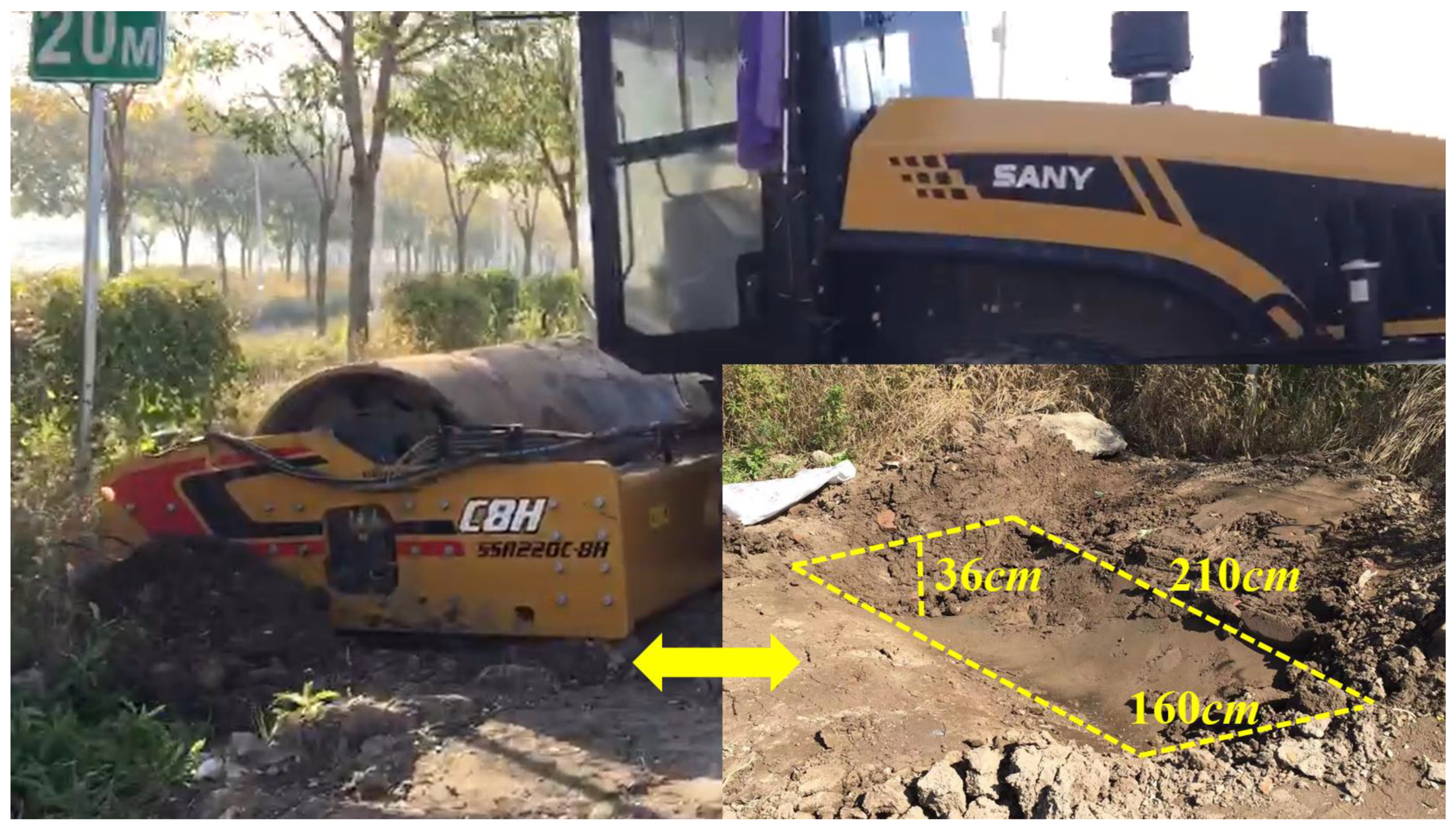
Figure 1. Representative field case of a UARR becoming entrapped on a mud pit.
Machines 14 00079 g001
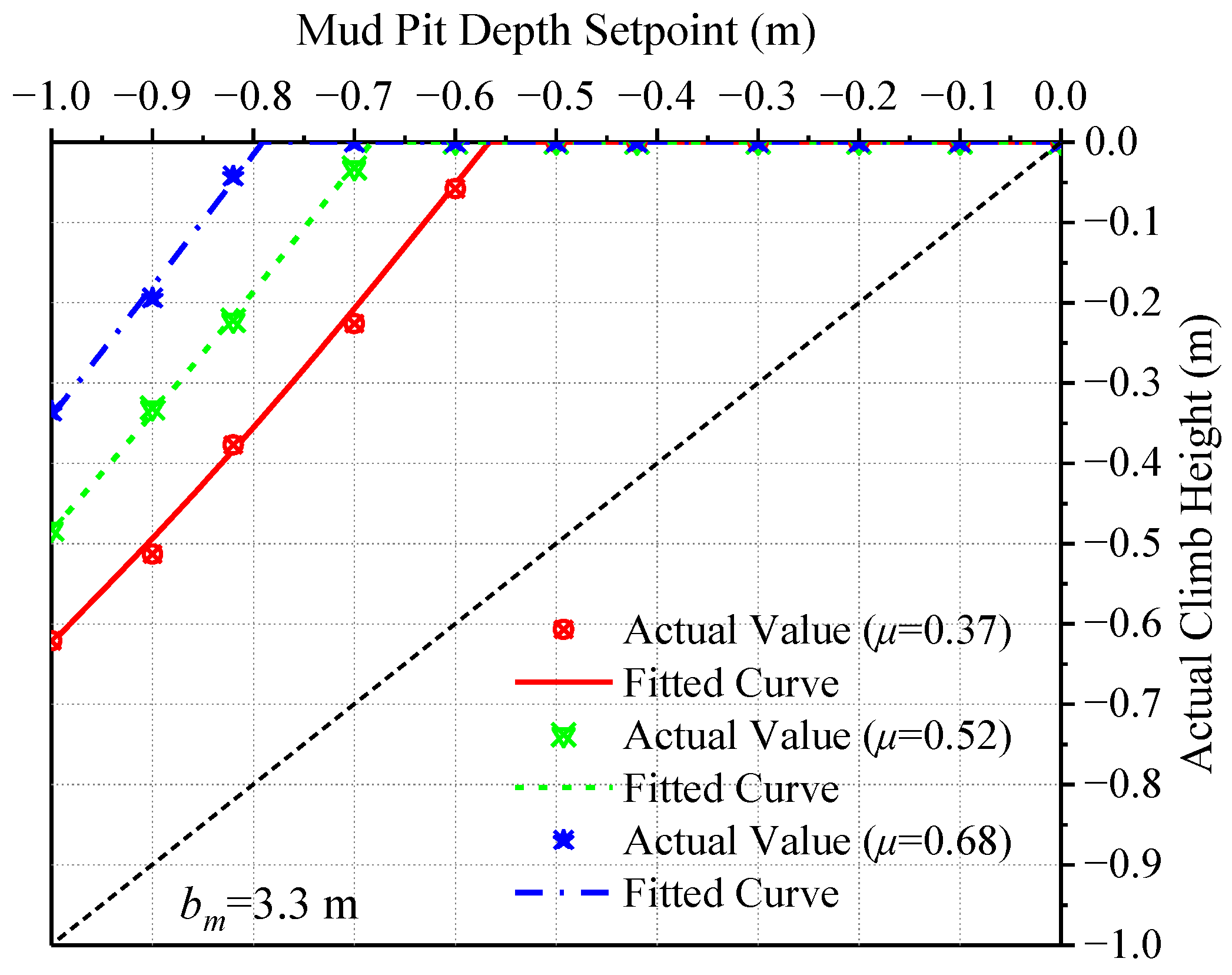
Figure 2. Architecture of the physics-based simulation platform for a UARR.
Machines 14 00079 g002
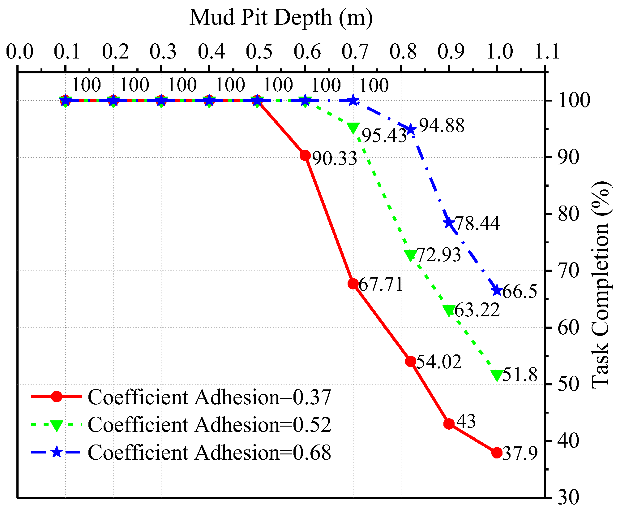
Figure 3. Hydraulic steering subsystem.
Machines 14 00079 g003
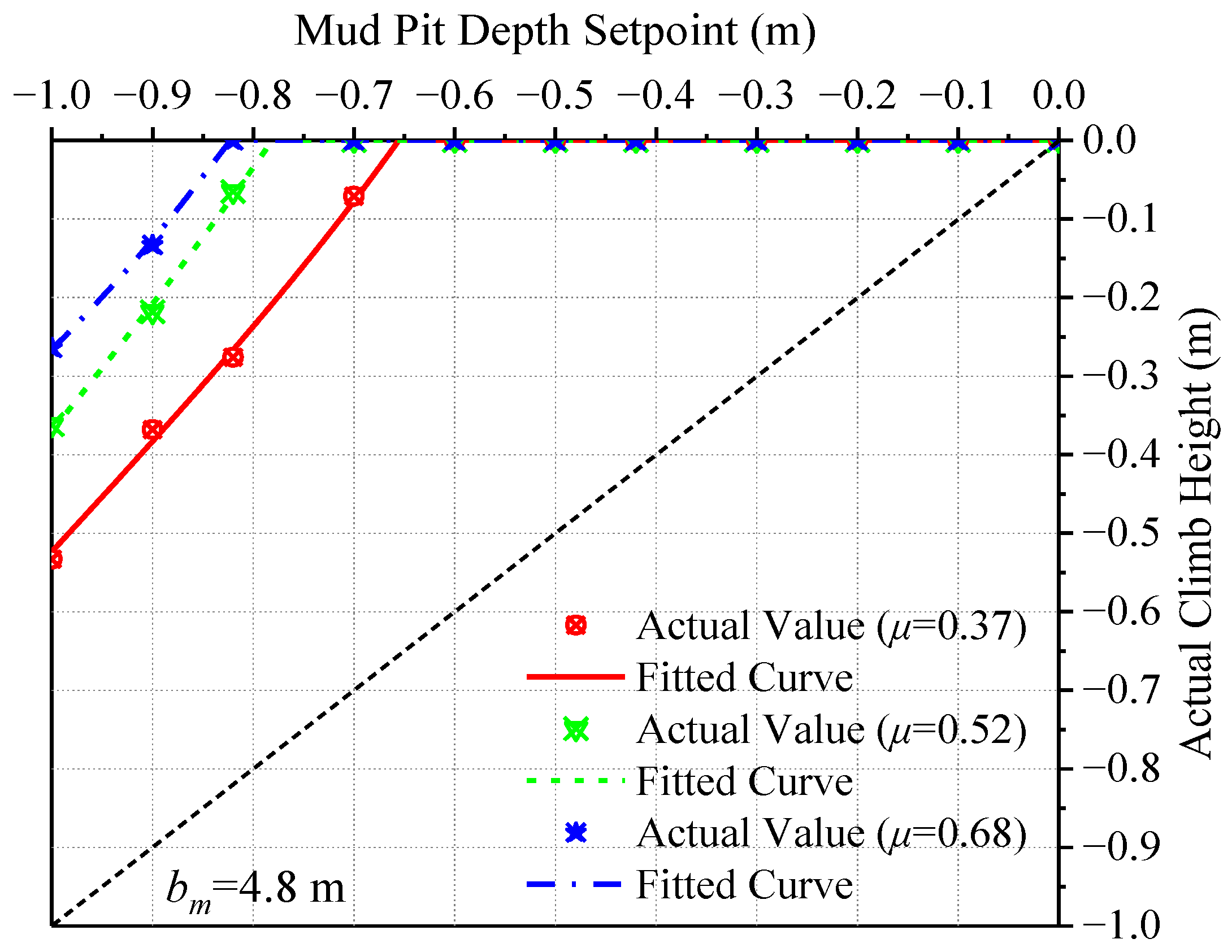
Figure 4. Wheel–terrain simulation submodel.
Machines 14 00079 g004
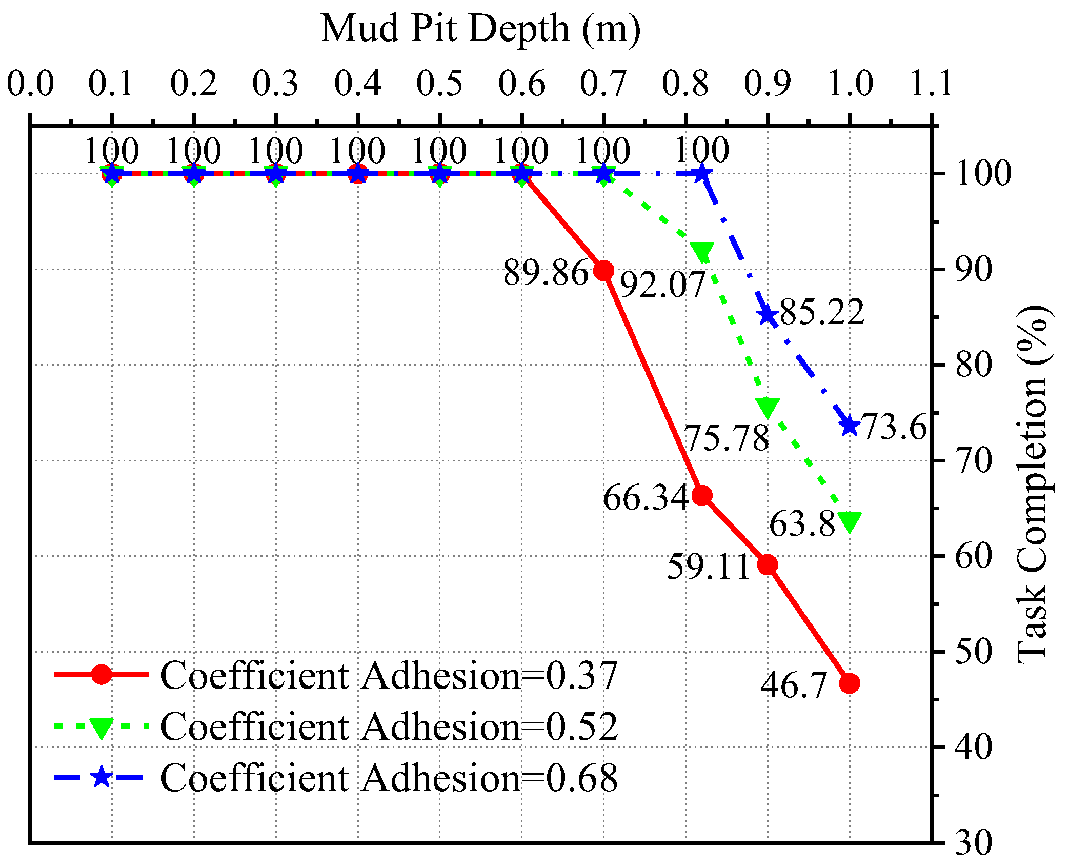
Figure 5. (a) Mud-pit surface with nominal adhesion μ b a s e = 0.35 and spatially varying friction; (b) additive adhesion perturbation map Δ μ [ 0.03 , + 0.03 ] .
Machines 14 00079 g005
Figure 6. Schematic of potential interference between the articulation joint and the pit edge during ascent.
Machines 14 00079 g006
Figure 7. Three-dimensional rendering of the simulation environment with a parametric mud pit (short semi-axis b m and depth d indicated).
Machines 14 00079 g007
Figure 8. Continuous “S”-shaped steering trajectory on dry soil.
Machines 14 00079 g008
Figure 9. Comparison of measured and simulated continuous “S”-shaped trajectory.
Machines 14 00079 g009
Figure 10. Comparison of measured and simulated key attitude angles during “S”-shaped steering.
Machines 14 00079 g010
Figure 11. Comparison of measured and simulated responses under wet soil road conditions.
Machines 14 00079 g011
Figure 12. Overall closed-loop control architecture with TAMPO embedded.
Machines 14 00079 g012
Figure 13. TAMPO framework.
Machines 14 00079 g013
Figure 14. Training-process comparison of different DRL algorithms.
Machines 14 00079 g014
Figure 15. Success rate (S.R.) of different algorithms on the test set.
Machines 14 00079 g015
Figure 16. Average escape time (A.E.T.) of different algorithms on the test set.
Machines 14 00079 g016
Figure 17. Algorithm success rate by difficulty level.
Machines 14 00079 g017
Figure 18. Comparison of training processes for TAMPO ablation variants.
Machines 14 00079 g018
Figure 19. Final success rates of TAMPO ablation variants on test sets.
Machines 14 00079 g019
Figure 20. Ablation variants algorithm success rate by difficulty level.
Machines 14 00079 g020
Figure 21. Three-dimensional escape trajectories of different algorithms in easy scenario.
Machines 14 00079 g021
Figure 22. Climb height vs. time curves of different algorithms in easy scenario.
Machines 14 00079 g022
Figure 23. Estimation of adhesion coefficient along trajectories in easy scenario.
Machines 14 00079 g023
Figure 24. Comparison of terrain interaction performance in easy scenario.
Machines 14 00079 g024
Figure 27. Estimation of adhesion coefficient along trajectories in medium scenario.
Machines 14 00079 g027
Figure 28. Comparison of terrain interaction performance in medium scenario.
Machines 14 00079 g028
Figure 31. Estimation of adhesion coefficient along trajectories in hard scenario.
Machines 14 00079 g031
Figure 32. Comparison of terrain interaction performance in hard scenario.
Machines 14 00079 g032
Figure 33. Performance map of TAMPO in scenarios with narrow pit opening ( b m = 1.8   m ).
Machines 14 00079 g033
Figure 34. Task completion rate of TAMPO in scenarios with narrow pit opening ( b m = 1.8   m ).
Machines 14 00079 g034
Figure 35. Performance map of TAMPO in scenarios with medium pit opening ( b m = 3.3   m ).
Machines 14 00079 g035
Figure 36. Task completion rate of TAMPO in scenarios with medium pit opening ( b m = 3.3   m ).
Machines 14 00079 g036
Figure 37. Performance map of TAMPO in scenarios with wide pit opening (bm = 4.8 m).
Machines 14 00079 g037
Figure 38. Task completion rate of TAMPO in scenarios with wide pit opening (bm = 4.8 m).
Machines 14 00079 g038
Table 1. Principal physical and geometric parameters of the front and rear frames.
ComponentParameterValueUnit
Front frameMass5200kg
CG height (relative to ground)780mm
CG longitudinal position (relative to articulation)1425mm
CG lateral position (relative to articulation)0mm
Moment of inertia about x-axis1841kg·m2
Moment of inertia about y-axis2358kg·m2
Moment of inertia about z-axis3695kg·m2
Rear frameMass6750kg
CG height (relative to ground)880mm
CG longitudinal position (relative to articulation)1530mm
CG lateral position (relative to articulation)0mm
Moment of inertia about x-axis2731kg·m2
Moment of inertia about y-axis3158kg·m2
Moment of inertia about z-axis5233kg·m2
Table 2. Principal physical and geometric parameters of the hydraulic steering subsystem.
ParameterValueUnit
Steering pump displacement80~500cc/r
Inlet pressure20MPa
Cylinder stroke455mm
Cylinder bore100mm
Piston-rod travel265mm
Piston-rod diameter57.3mm
Hydraulic line inner diameter24mm
Table 3. Principal physical and geometric parameters of the drum and rear wheels.
ComponentParameterValueUnit
Front drumDiameter1600mm
Steel width2130mm
Mass9400kg
CG height (with respect to ground)800mm
CG longitudinal position (with respect to articulation)1500mm
CG lateral position (with respect to articulation)0mm
Rear wheelsDiameter1500mm
Tire width595mm
Track width1980mm
Mass (per wheel assembly)650kg
CG height (with respect to ground)750mm
CG longitudinal position (with respect to articulation)1680mm
CG lateral position (with respect to articulation)0mm
Table 4. Statistics of lateral deviation peaks at turning points.
Turn IndexMeasured Peak YSimulated Peak YNormalized Error (% of Range)
1870.18870.251.56%
2873.20873.312.44%
3870.59870.753.56%
4872.80872.871.56%
5870.51870.561.11%
6871.75871.681.56%
7869.52869.432.00%
8871.03870.785.56%
9868.70868.514.22%
10871.56871.403.56%
11870.48870.431.11%
12872.78872.872.00%
13871.90872.012.44%
Table 5. Hyperparameters for TAMPO neural-network training.
ParameterSymbolValueDescription
Discount factorγ0.99Trades off long- vs. short-term return
Actor learning rateηθ0.0003Adam step size for policy network
Critic learning rateηψ0.001Adam step size for value network
GAE parameterλ0.95Bias-variance trade-off in generalized advantage estimation
Initial entropy coefficientα00.2Initial value for adaptive entropy
Entropy decay rateβH0.0001Exponential time-decay factor for α
Minimum entropy coefficientαmin0.01Lower bound to preserve exploration
Weight: terrain difficultyλD0.5Weight in adaptive exploration scheduler
Weight: progress efficacyλη0.2Weight in adaptive exploration scheduler
Weight: value uncertaintyλV0.3Weight in adaptive exploration scheduler
Polyak averaging factorτ0.005Soft-update rate for target value network
Max steps per episodeTmax256Maximum environment interactions per episode
Table 6. Comparison of the overall performance of different algorithms on two test sets.
DRL AlgorithmInterpolation Test Set Ω t e s t interp Extrapolation Test Set Ω t e s t extrap
S.R. (%)A.E.T. (s)A.C.R.S.R. (%)A.E.T. (s)A.C.R.
TAMPO70.83 ± 1.7414.92 ± 0.59428.7660.00 ± 1.8617.56 ± 0.59389.15
SAC61.46 ± 3.1616.77 ± 0.82346.5350.00 ± 2.5320.03 ± 1.74290.73
R.P.9.37 ↓1.85 ↑82.23 ↓10.00 ↓2.47 ↑98.42 ↓
PPO54.17 ± 3.5518.46 ± 1.35269.2745.55 ± 2.8122.29 ± 2.21215.48
R.P.16.66 ↓3.54 ↑159.49 ↓14.45 ↓4.73 ↑173.67 ↓
DDPG43.75 ± 4.3221.37 ± 1.70251.8237.78 ± 2.9023.29 ± 2.07196.92
R.P.27.08 ↓6.45 ↑176.94 ↓22.22 ↓5.73 ↑192.23 ↓
Note: R.P. denotes the relative performance of the baseline algorithms compared to TAMPO.
Table 7. Actual climb heights of TAMPO in scenarios with narrow pit opening ( b m = 1.8   m ).
Pit Opening Dimension (m)Depth Setpoint (m)Actual Climb Height (m)
1.80 µ base = 0.37 µ base = 0.52 µ base = 0.68
−1.000.2580.4130.558
−0.900.2790.4050.603
−0.820.2520.4780.614
−0.700.3340.4920.674
−0.600.3360.5790.600
−0.500.4290.5000.500
−0.420.4200.4200.420
−0.300.3000.3000.300
−0.200.2000.2000.200
−0.100.1000.1000.100
Table 8. Actual climb heights of TAMPO in scenarios with medium pit opening ( b m = 3.3   m ).
Pit Opening Dimension (m)Depth Setpoint (m)Actual Climb Height (m)
3.30 µ base = 0.37 µ base = 0.52 µ base = 0.68
−1.000.3790.5180.665
−0.900.3870.5690.706
−0.820.4430.5980.778
−0.700.4740.6680.700
−0.600.5420.6000.600
−0.500.5000.5000.500
−0.420.4200.4200.420
−0.300.3000.3000.300
−0.200.2000.2000.200
−0.100.1000.1000.100
Table 9. Actual climb heights of TAMPO in scenarios with wide pit opening ( b m = 4.8   m ).
Pit Opening Dimension (m)Depth Setpoint (m)Actual Climb Height (m)
3.30 µ base = 0.37 µ base = 0.52 µ base = 0.68
−1.000.3790.5180.665
−0.900.3870.5690.706
−0.820.4430.5980.778
−0.700.4740.6680.700
−0.600.5420.6000.600
−0.500.5000.5000.500
−0.420.4200.4200.420
−0.300.3000.3000.300
−0.200.2000.2000.200
−0.100.1000.1000.100
Disclaimer/Publisher’s Note: The statements, opinions and data contained in all publications are solely those of the individual author(s) and contributor(s) and not of MDPI and/or the editor(s). MDPI and/or the editor(s) disclaim responsibility for any injury to people or property resulting from any ideas, methods, instructions or products referred to in the content.