Analysis, Modeling, and Simulation of a Rocker–Bogie System Overcoming a Harmonic Bump

Abstract

Rocker–bogie suspension systems have been extensively employed in planetary exploration rovers due to their ability to traverse highly irregular terrains while maintaining ground contact. Traditionally, their mechanical behavior has been analyzed using quasi-static models, given the low operational speeds typical of space missions. However, similar configurations are now being proposed for terrestrial applications in agriculture, defense, and logistics, where higher traversal speeds and more varied terrain conditions require a deeper understanding of the system’s dynamic response. This study analyzes some aspects of the kinematic and dynamic behavior of a rover with rocker–bogie suspension while traversing an obstacle with a harmonic profile. Both quasi-static and dynamic simulations are conducted, focusing on the time-varying contact forces at the wheels. Key findings include identifying the rate at which load reduction at which the load on one wheel becomes zero and the wheel tends to lift off the ground. These threshold speeds are mapped as a function of height and wavelength of the bump, providing design insights for applications requiring higher traversal speeds on uneven terrain. The analysis may also prove valuable for rovers equipped with visual sensor systems capable of mapping their surroundings and identifying obstacles, to determine whether they can be traversed and, if so, at what maximum speed. An experimental investigation was conducted with a small-scale rover to verify the theoretical results, for which the threshold speed was found to be 0.3 m/s, calculated for h = 16 mm and λ = 80 mm.

1. Introduction

Rovers equipped with rocker–bogie suspension were first introduced in space missions starting in 1997 [1,2], thanks to their ability to move reliably on uneven terrain [3,4], a performance that is difficult to achieve with conventional four-wheeled vehicles [5]. Their effectiveness comes from having six-wheel drive and a kinematic suspension system capable of maintaining contact with the ground [6,7], even in the presence of obstacles with a height approximately twice the diameter of the wheels [4,8].

Traditionally, the mechanical study of these systems has been conducted with a quasi-static approach, due to the low speed adopted in space applications. The operating speeds of rovers are generally limited by the characteristics of the gear-motors installed in the wheel hubs, which prioritize torque delivery over speed. However, in different conditions, it may be desirable for the rover to proceed faster.

More recently, these rovers have also been proposed for terrestrial applications, in agricultural [9,10,11,12], military [13], logistics settings, and other applications [14] where the possibility of operating at higher speeds on smoother surfaces is appreciated. Innovations associated with the design, production, and control of these robotic systems are indicated in [15].

One of the most significant challenges faced by rovers, given their intended operation in environments characterized by irregular surfaces, is the management of obstacles encountered along their path. To improve obstacle-climbing performance, some papers focus on optimizing the geometry of the suspension links [16], the insertion of preloaded elastic elements between the rocker and the bogie [7], or the possibility of shifting the position of the center of gravity [17].

If the rover is equipped with a vision system capable of detecting obstacles along its path, it must be able to assess, based on the obstacle’s nature and geometry, whether it is more convenient to bypass or overcome it. Avoiding obstacles requires reprogramming the path [18] and the adoption of visual sensors, such as RGB-D cameras, that have been shown to be particularly effective for environment mapping and obstacle recognition [19]. These are frequently complemented by LiDAR sensors, which enhance the robustness and reliability of navigation algorithms [20]. Algorithms are commonly based on neural networks [21] or fuzzy logic [22] and are often combined with other techniques to improve accuracy [23]. In more sophisticated systems, these may be replaced or augmented by approaches based on Reinforcement Learning [24], which allow the rover to learn optimal navigation strategies through interaction with the environment.

Overcoming the obstacle directly is preferable, as it saves time by avoiding reprogramming the path. Furthermore, choosing an alternative path does not guarantee the absence of other hard obstacles on the new path, introducing further operational uncertainty. Therefore, this choice, resulting in a deviation from the originally defined path, is often characterized by higher energy consumption.

The ability to directly overcome obstacles requires greater mechanical complexity in the rover design. In this context, the six-wheeled configuration, equipped with a rocker–bogie suspension, has proven to be a particularly effective solution. This system allows the rover to adapt to uneven terrain, distributing load quite evenly and maintaining stability even when overcoming significant obstacles, without compromising traction. If the obstacle can be overcome, the rover must be able to evaluate the traversal method considering how its configuration and ground reactions on the wheels could vary, affecting grip conditions. A more in-depth analysis would require knowledge of the terrain’s characteristics, which could be soft or slippery [25]. However, a simplified analysis can be conducted by assuming that both the ground and the rover’s constituent bodies are rigid.

Many papers address the problem of overcoming step obstacles [26,27] or bump obstacles [28]. The first consists of two horizontal surfaces at different elevations, connected by a vertical or near-vertical wall. Completely traversing this obstacle requires the entire rover to move from one reference plane to another, changing its operating altitude. This type of obstacle is useful for evaluating the locomotion system’s ability to negotiate sharp and abrupt changes in height. The bump obstacle is characterized by a localized elevation of the travel plane, with a length shorter than the vehicle’s wheelbase; completely traversing this type of obstacle does not change the rover’s operating altitude. The most used bumps are those with linear ramps and plateaus, triangular ones or those with circular or parabolic profiles.

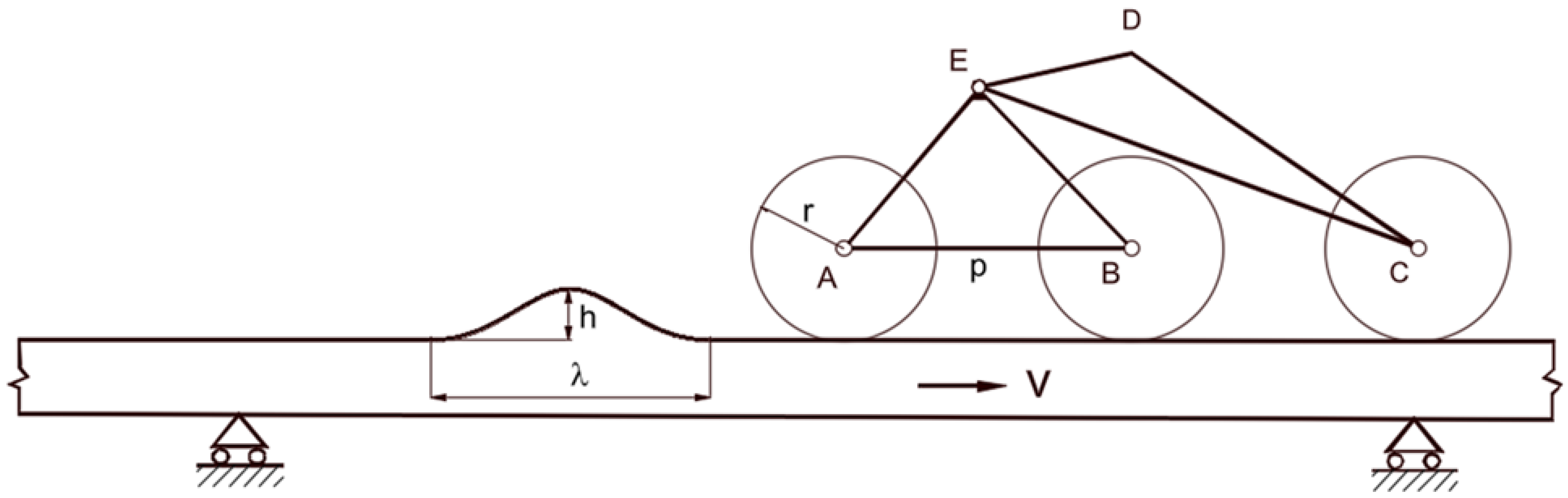
In the following, we consider a bump with a harmonic profile that is continuous and without edges, which in nature are generally smoothed or eroded. Figure 1 shows a single bump with a harmonic profile. The term harmonic bump is introduced in this paper to denote a localized obstacle with a sinusoidal profile and wavelength smaller than the wheelbase. This terminology is intended to provide a concise and descriptive reference for this specific geometric configuration that is controlled by two parameters: height and wavelength (h, λ). Short wavelengths, coupled with significant bump heights, can make the obstacle particularly treacherous. The resulting steep profiles may compromise wheel traction, increasing the risk of slippage or loss of contact. Furthermore, since the length of the obstacle is less than the wheelbase, it could fit between two consecutive wheels, causing the rover to stall.

The paper aims to determine the ground constraint reactions as a function of the position of the wheels on the bump. Rovers often move at very low speeds, so quasi-static analyses are sufficient to determine their behavior. As speed increases, inertial effects become more important, and the vertical inertial force can even exceed the force of gravity; the combination of vertical and horizontal inertial forces can cause the wheel to lift off the ground. Agricultural robots typically operate at low speeds, but their maximum speed is between 0.6 and 2.8 m/s [29,30]; similar robots used in logistics, which therefore move on prepared terrain, can advance even faster.

In this paper, a simple model is proposed for determining the forward speed beyond which the wheel can lose contact with the ground. Wheel lift can lead to a loss of traction and reduced directional control, particularly in skid-steering vehicles. Upon re-contact with the ground, the impact may generate harmful vibrations and induce stress on onboard instrumentation. Additionally, navigation accuracy can be compromised if position estimation relies partly on wheel rotation.

Numerical simulations were conducted using a multibody software platform to evaluate the rover’s behavior under hypothesized operating conditions. This modeling approach enables the generation of performance maps, providing a preliminary assessment of the rover’s capability to traverse obstacles. Finally, the paper presents experimental investigations carried out with a small-scale rover as it crosses a bump featuring a harmonic profile.

2. Rover Reference Model

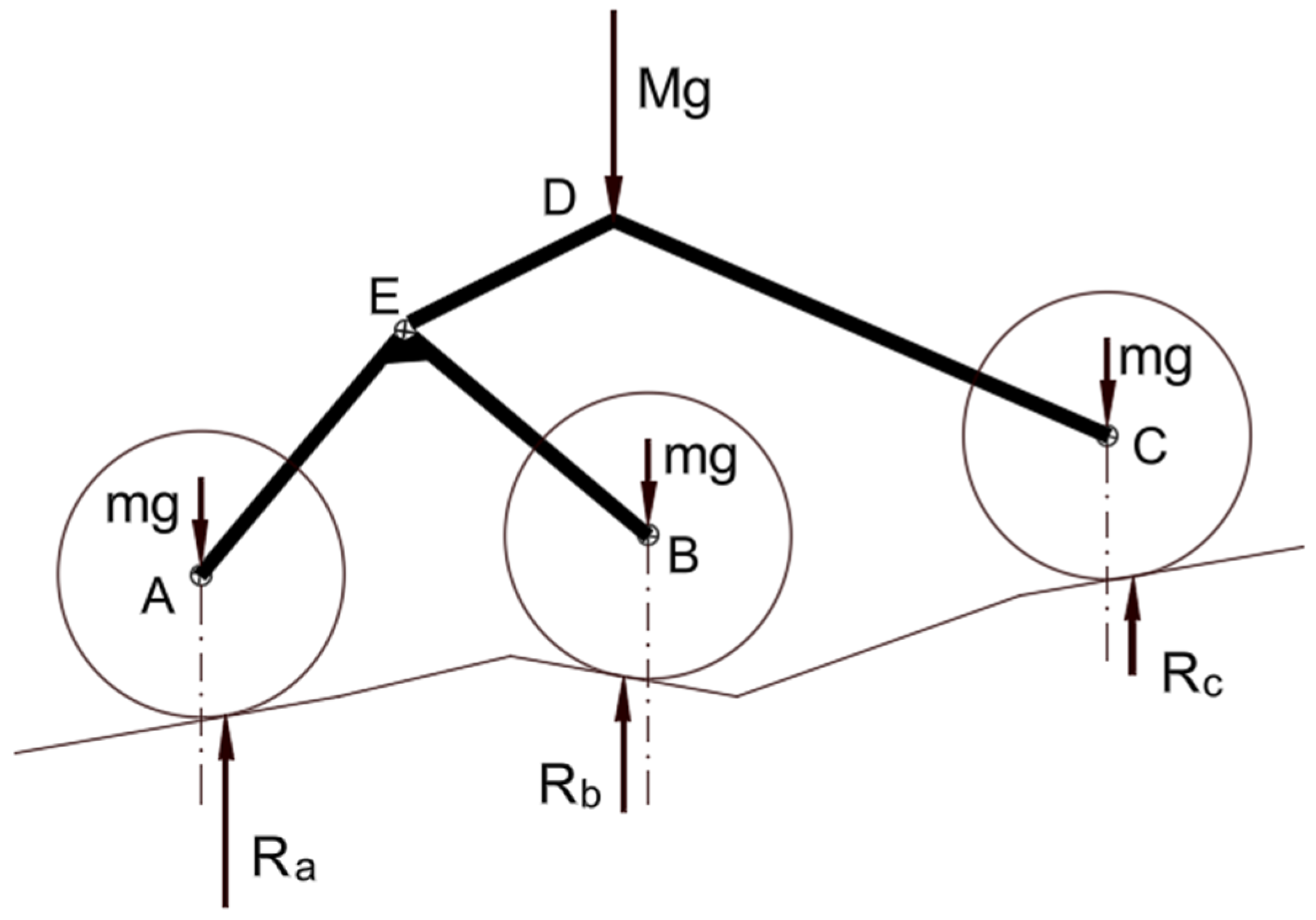
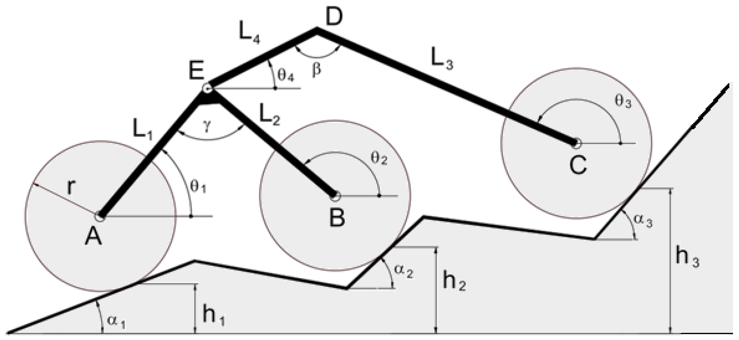
The study is carried out using the classical two-dimensional model represented in Figure 2. It is assumed that the center of gravity of the body is located at point D of the rocker and that the centers of gravity of the motorized wheels are in the centers of the respective wheels (points A, B, C). The lengths of the suspension links are chosen so that the load acting on the wheels is the same if the rover is placed with its wheels at the same level on a flat surface. The adoption of a kinematic model [7] allows to identify the position assumed by the rover as a function of the altitudes of the contact point h_i of each wheel and the ground inclination α_i at the same point. The model provides as output the angles θ_i that the suspension links form with the horizontal direction and, therefore, the coordinates of representative points of the model. The knowledge of the rover’s pose allows to solve the static problem and obtain the ground reactions.

The ground reactions have been scaled so that, in static conditions, their vertical resultant is equal to 300 N. Consequently, if the wheels are all at the same height on a horizontal plane, the normalized ground reaction on each wheel is 100 N. Rescaling makes comparative data analysis simpler as it allows to easily evaluate the percentage changes in reactions as the soil profile varies.

In the following, a small-sized rover having the geometric and inertial characteristics indicated in

Table 1. Rover physical parameters.

L1 = L2 (mm)	L3 (mm)	L4 (mm)	p (mm)	r (mm)	$\mathsf{\gamma }$ (deg)	$\mathsf{\beta }$ (deg)	m (kg)	M (kg)
72.5	123	54	102.5	32.5	90	120	0.06	0.50

is considered; m and M are the mass of the wheel-motor assembly and that of the body, respectively; p is the distance between the axes of the bogie wheels which is equal to the distance between wheels B and C when the rover is on a flat, horizontal surface. As an example, Figure 3 shows the rover configuration and the corresponding vertical ground reactions for the input data reported in

Table 2. Soil characteristics and a qi angles defining the rover pose.

h1 (mm)	α1 (°)	h2 (mm)	α2 (°)	h3 (mm)	α3 (°)	θ1 (°)	θ2 (°)	θ3 (°)	θ4 (°)
15	20	9	−10	32	10	49.7	139.7	154.0	34.0

. The same table shows the angles θi assumed by the suspension links.

3. Wheel on Harmonic Bump

It is assumed that the rover must overcome a bump with a harmonic profile of height h and wavelength λ, as shown in Figure 4. The profile equation is expressed by the following function:

$$z\left(x\right)={\displaystyle \frac{h}{2}} \left(1-\mathrm{c}\mathrm{o}\mathrm{s}\left({\omega }_{s}x\right)\right)$$

(1)

being ${\omega }_s={\displaystyle \frac{2\pi }{\lambda }}$, the circular spatial frequency of the bump profile, expressed in rad/m.

To this end, it is assumed that the rover rests on the ground characterized by the presence of a bump, which moves in a horizontal direction with constant speed. The bump profile acts as a geometric constraint and as long as the contact with the wheels takes place with the flat part before the bump, since there are no other horizontal actions, the rocker and bogie remain stationary in the same pose, while the wheels roll due to the motion of the profile. When the harmonic profile meets the wheels, the rover’s configuration changes and the reactions on the wheels also change. For small values of the velocity, since the inertial forces are negligible, for each position of the profile, the reactions assume values equal to those deriving from static equilibrium.

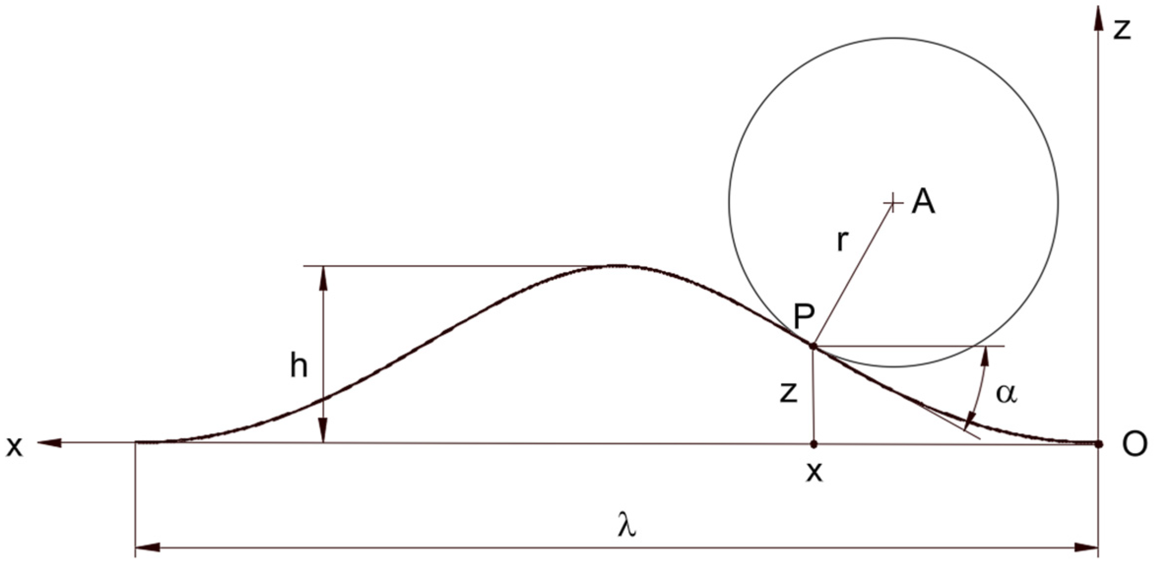
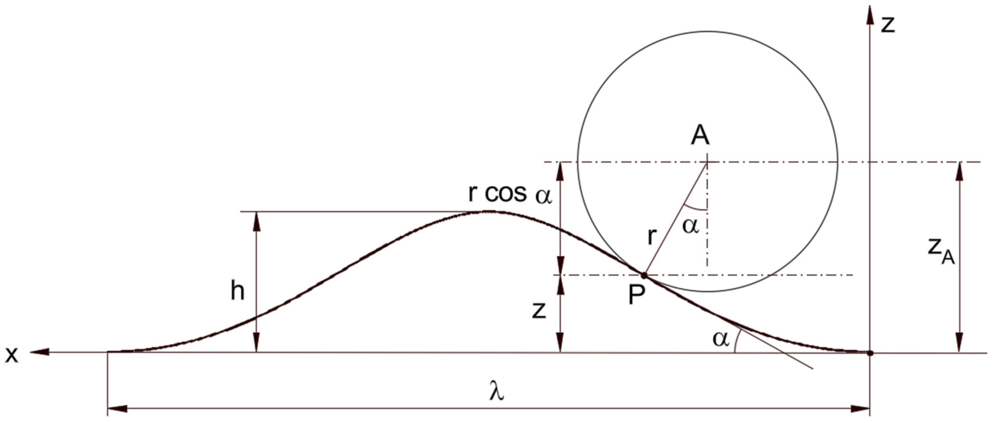
To evaluate the relative position of each wheel with respect to the harmonic profile, refer to the diagram in Figure 5. A reference system is considered with its origin at the starting point of the harmonic sliding profile; (x, z) are the coordinates of the point P of contact between the wheel and the bump profile. The common tangent of the two bodies is inclined at an angle α with respect to the x-axis. What is reported below for wheel A is also valid for the other wheels of the rover.

Assuming the speed of the sliding profile to be constant, it is x = vt; the vertical displacement of the wheel–bump contact point P, as a function of time, is

$$z\left(t\right)={\displaystyle \frac{h}{2}} \left[1-\mathrm{c}\mathrm{o}\mathrm{s}\left({\omega }_{s}vt\right)\right]$$

(2)

being ${\omega }_{s}v=2\pi v/\lambda$, the rotating frequency in rad/s of point P vertical motion. The wheel remains engaged with the bump for the time T equal to

$$T={\displaystyle \frac{2\pi }{{\omega }_{s}v}}=\lambda /v.$$

(3)

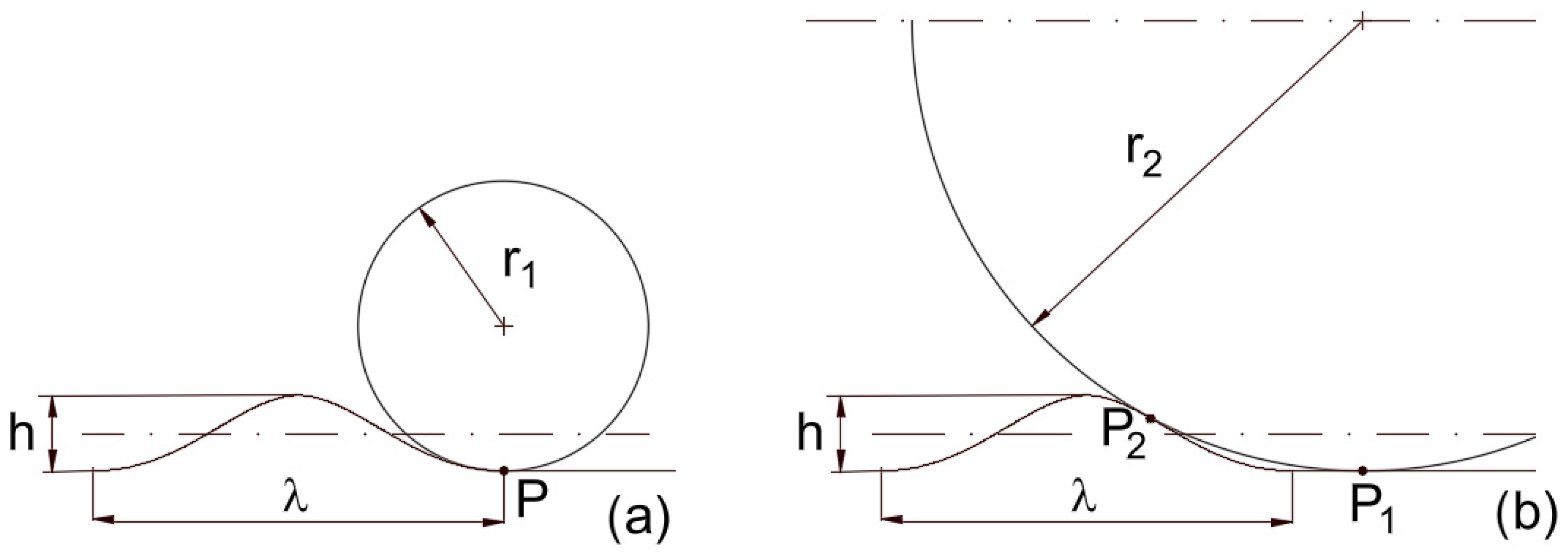
It should be noted that, how represented in Figure 6, if the radius r of the wheel is less than the minimum radius of curvature of the bump profile (r ≤ ρ_min), the wheel rolls over the bump while maintaining continuous contact (Figure 6a); if r > ρ_min, in the phase of approach to the bump, contact can occur simultaneously at two points (Figure 6b); the wheel “jumps” from a point P₁, on the horizontal part before the bump, to a point P₂ in a higher position along the harmonic profile. This circumstance generates a discontinuity in the vertical motion of the wheel, accompanied by a sudden change in the α angle and the coordinates of the center of the wheel. These conditions can lead to impulsive reactions and a temporary loss of grip. However, in practice, the deformability of the surfaces involved helps to make this step less critical, attenuating the associated dynamic effects.

By particularizing the expression of the radius of curvature of a plane curve for the case of the harmonic profile, we have

$$\rho \left(x\right)={\displaystyle \frac{{\left[1+{\left(z^{\prime }\left(x\right)\right)}^2\right]}^{3/2}}{\left|z^{″}\left(x\right)\right|}}={\displaystyle \frac{{\left[1+{\left(\frac{h}{2}{\omega }_s\sin \left({\omega }_{s}x\right)\right)}^2\right]}^{3/2}}{\left|\frac{h}{2}{\omega }_s^2\cos \left({\omega }_{s}x\right)\right|}}={\displaystyle \frac{{\left[1+{\left(\frac{h\pi }{\lambda }sin(\frac{2\pi }{\lambda }x)\right)}^2\right]}^{3/2}}{\left|\frac{2h{\pi }^2}{{\lambda }^2}cos(\frac{2\pi }{\lambda }x)\right|}}$$

(4)

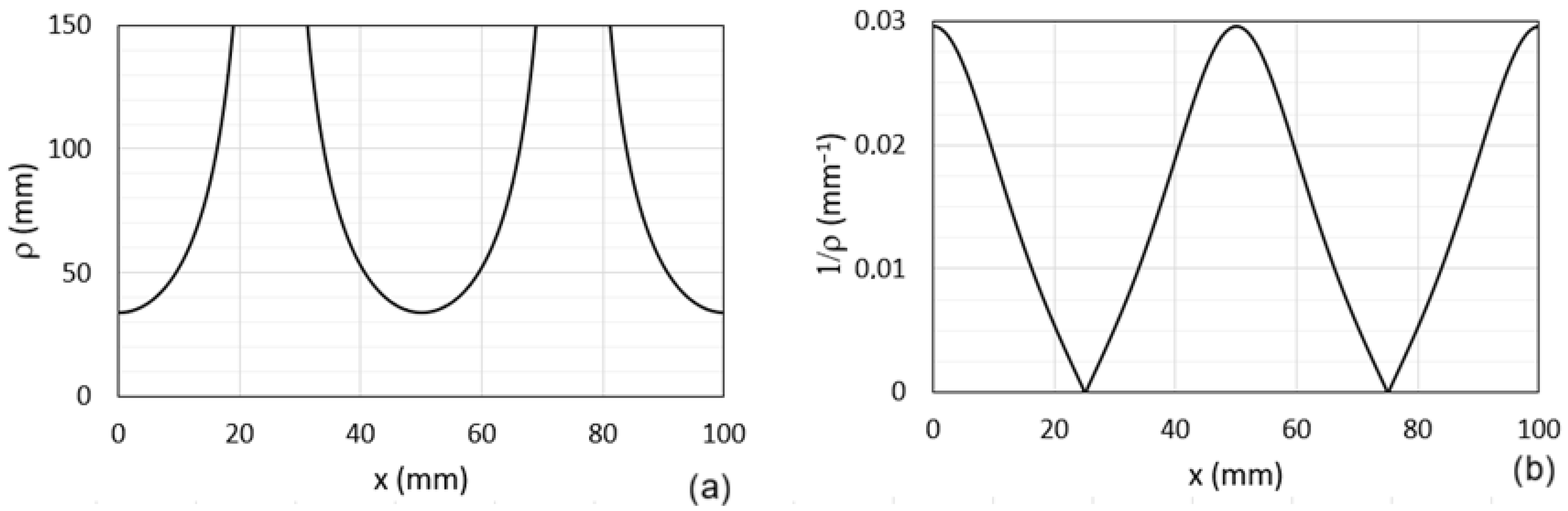
Figure 7 shows the diagram of the radius of curvature of the profile and the curvature. Since the focus is on the minimum radius of curvature of the harmonic profile, the transition radius between the curved segment and the adjacent flat regions—where the curvature is zero and the radius theoretically infinite—is not considered. The diagram shows that the minimum radius of curvature occurs at the beginning of the profile (x = 0) and is

$${\rho }_{min}=\rho \left(0\right)={\displaystyle \frac{{\lambda }^2}{2h{\pi }^2}}$$

(5)

If r(0) ≥ r, in the generic contact point of x-axis, with reference to Figure 8, the coordinates of the wheel center A are

$$x_A\left(x\right)=x-r sin\alpha$$

(6)

$$z_A\left(x\right)=z+r cos\alpha ={\displaystyle \frac{h}{2}} \left[1-\mathrm{c}\mathrm{o}\mathrm{s}\left({\omega }_{s}x\right)\right]+r cos\alpha$$

(7)

The angle α = α(x), by which the tangent of the bump profile is inclined at the point of contact of the wheel, is evaluated considering that

$$u=\tan \alpha ={\displaystyle \frac{dz}{dx}}={\omega }_s{\displaystyle \frac{h}{2}}\sin \left({\omega }_{s}x\right)={\displaystyle \frac{\pi h}{\lambda }}\sin \left({\displaystyle \frac{2\pi }{\lambda }} x\right)$$

(8)

with

$$\alpha =\mathrm{a}\mathrm{r}\mathrm{c}\mathrm{t}\mathrm{a}\mathrm{n}\left(u\right)$$

(9)

By means of the fundamental trigonometric expressions, we have

$$sin\alpha ={\displaystyle \frac{tan\alpha }{\sqrt{1+{tan}^2\alpha }}}={\displaystyle \frac{u}{\sqrt{1+u^2}}}={\displaystyle \frac{{\omega }_s\frac{h}{2}\mathit{sin}\left({\omega }_s x\right)}{\sqrt{1+{\left({\omega }_s\frac{h}{2}\right)}^2{\sin }^2\left({\omega }_s x\right)}}};$$

(10)

$$cos\alpha ={\displaystyle \frac{1}{\sqrt{1+{tan}^2\alpha }}}={\displaystyle \frac{1}{\sqrt{1+u^2}}}={\displaystyle \frac{1}{\sqrt{1+{\left({\omega }_s\frac{h}{2}\right)}^2{\sin }^2\left({\omega }_s x\right)}}}$$

(11)

Therefore, the coordinates reported in Equations (6) and (7) can be expressed as follows:

$$x_A\left(x\right)=x-r sin\alpha \left(x\right)=x-r {\displaystyle \frac{{\omega }_s\frac{h}{2}\mathit{sin}\left({\omega }_s x\right)}{\sqrt{1+{\left({\omega }_s\frac{h}{2}\right)}^2· \frac{1-\cos \left(2{\omega }_s x\right)}{2}}}}$$

(12)

$$z_A\left(x\right)=z(x)+r cos\alpha (x)={\displaystyle \frac{h}{2}} \left[1-\mathrm{c}\mathrm{o}\mathrm{s}\left({\omega }_{s}x\right)\right]+{\displaystyle \frac{r}{\sqrt{1+{\left({\omega }_s\frac{h}{2}\right)}^2· \frac{1-\cos \left(2{\omega }_s x\right)}{2}}}}$$

(13)

Therefore, for x = 0 (start of bump climbing), $z_A=r$ and for x = λ/2 it is $z_A=r+h$.

Both coordinates show a harmonic component with pulsation ${\omega }_s$, modulated in amplitude by a component with double pulsation.

The coordinates of the center can also be deduced by evaluating, for each value of x, the angle α, with Formula (9).

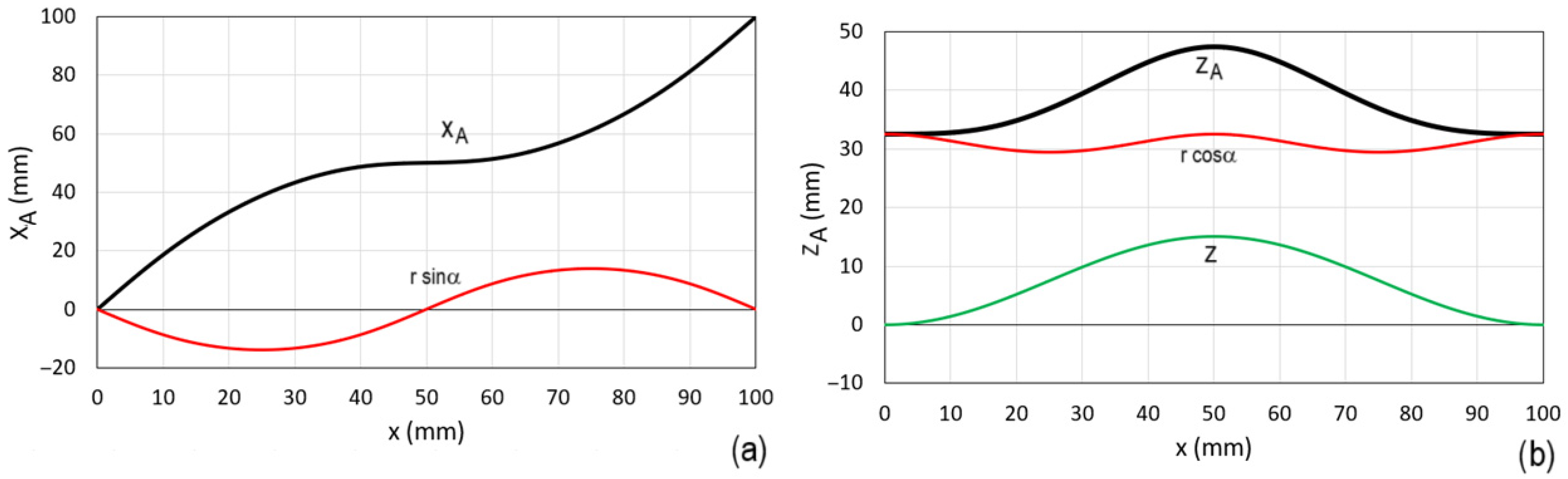
Figure 9 shows the coordinates of the center of the wheel moving on the profile, remaining in contact with it, depending on the displacement of the sliding profile, evaluated for λ = 100 mm, h = 15 mm, ${\omega }_s$ = 2π/λ = 62.8 rad/m, r = 32.5 mm. It follows that $\rho \left(0\right)=$ 33.8 mm, which is greater than the radius of the wheel.

4. Influence of the Wheel/Profile Contact Point on the Ground Reactions

For ρ(0) < r, if the rover passes the bump moving very slowly, the reactions of the ground on the wheels vary gradually and can be evaluated by considering a sequence of static conditions.

Since our aim is to evaluate the ground reactions both when the rover is stationary and when it moves at a constant speed, we consider a bump whose height is smaller than the length of the bogie links (h < L₁ = L₂). For such a value, the reaction on the wheel positioned at the crest of the bump becomes zero under static conditions.

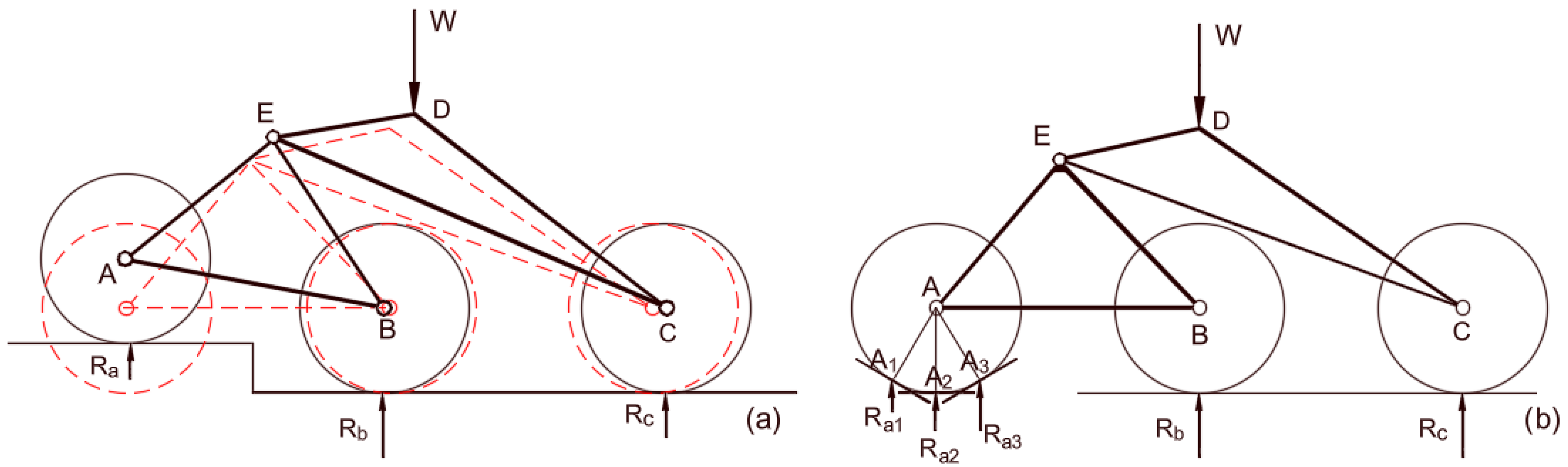
In Figure 10, it can be observed that, when one of the wheels engages with the bump, the bogie and the rocker are subjected to rotations (Figure 10a) that can be evaluated after obtaining, through a kinematic analysis [7], the positions of the centers of the three wheels and of point E:

$${\theta }_{bg}=arctan\left({\displaystyle \frac{Z_C-Z_B}{X_C-X_B}}\right); {\theta }_{rk}=arctan\left({\displaystyle \frac{Z_B-Z_E}{X_B-X_E}}\right)$$

(14)

The modified distance between the rover’s notable points also involves variations in the vertical reactions on the wheels. For example, lifting wheel A involves a clockwise rotation of both bogie and the rocker; rocker rotation causes wheel C to approach the line of action of the load W in D while hinge E moves away from the same line. Consequently, the load in C increases and that in E decreases. The load in E is mainly balanced by the wheel B which tends to move closer to the vertical line for E.

The distances between the contact points of the wheels also depend on the inclination of the ground at the contact points; for example, in Figure 10b, the wheels are all at the same level, but the contact of wheel A with the ground takes place at points with different inclinations of the ground (indicated by A1, A2, A3).

Equation (6) shows that the distance $x_A-x$ is variable with α(x) and that the maximum value depends on the radius of the wheel, the wavelength, and the height of the bump profile:

$$x_A-x=r sin\alpha =r \mathrm{s}\mathrm{i}\mathrm{n}\left[arctan{\displaystyle \frac{\pi h}{\lambda }}\sin \left({\displaystyle \frac{2\pi }{\lambda }} x\right)\right]$$

(15)

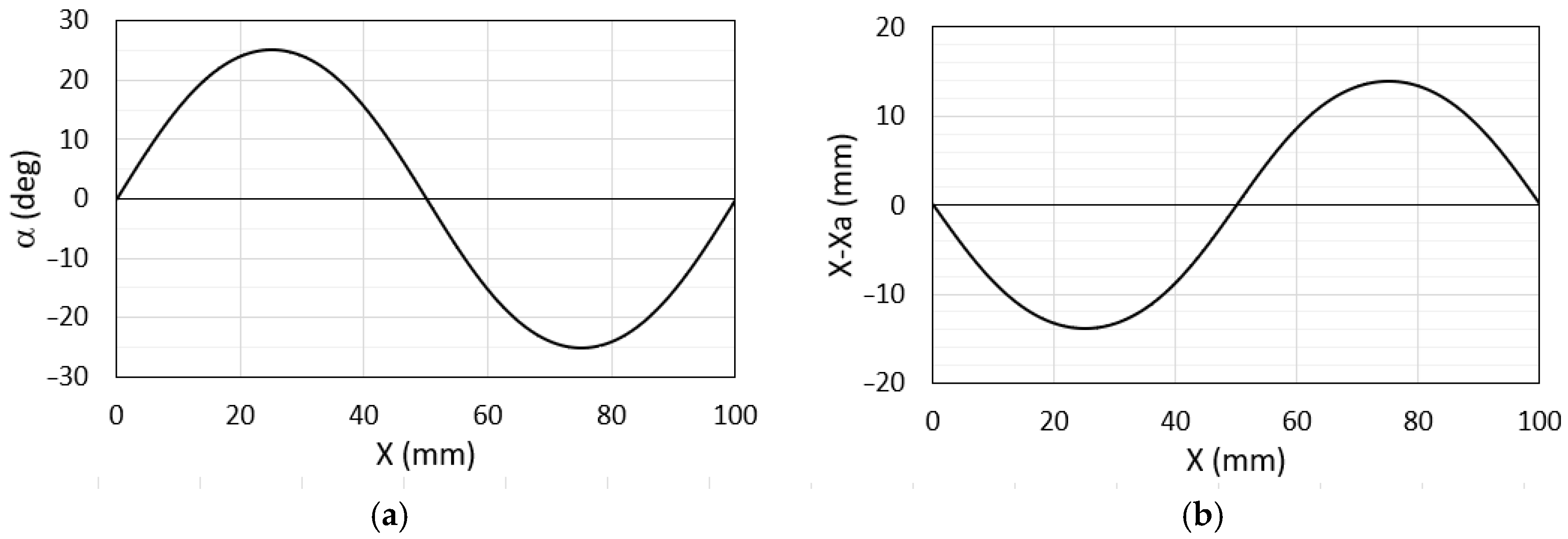
Figure 11 shows the trend of the angle α and the difference $x_A -x$, for λ = 100 mm, h = 15 mm, r = 32.5 mm.

Assigning the geometric characteristics of the soil profile, using kinematic analysis [7], it is possible to define the rover configuration, the location of the wheel-to-ground contact points, and the common tangent slope so that ground reactions can be evaluated. With reference to Figure 10b,

Table 3. Normalized vertical reactions as a function of the tangent inclination at the wheel–soil contact point.

Wheel	α1 (deg)	zA (mm)	Ra	Rb	Rc
A1	−25	0	94	107	100
A2	0	0	100	100	100
A3	+25	0	114	87	100

shows the normalized values of the vertical reactions in the case of a wheel at the same height but with different inclinations of the ground at the contact point. The vertical reaction at the point of contact of wheel A decreases if it moves away from the vertical for E.

Therefore, when wheel A overcomes the bump, there is a continuous variation in the level and inclination of the ground; in the ascent phase, due to the rotations of the bogie, the contact point moves forward (in the direction of motion) with respect to the wheel center, resulting in an increase in the load on wheel B, which is as large as the greater the inclination of the profile at the contact point. This variation in load can be considered beneficial; in fact, wheel A, which must be lifted, undergoes a reduction in load while wheel B can push the rover forward, without slipping, thanks to the increase in load. The wheel C undergoes slight variations in load. The opposite situation occurs when wheel A is descended from the bump, during which the loads on the wheels tend to return to their initial value.

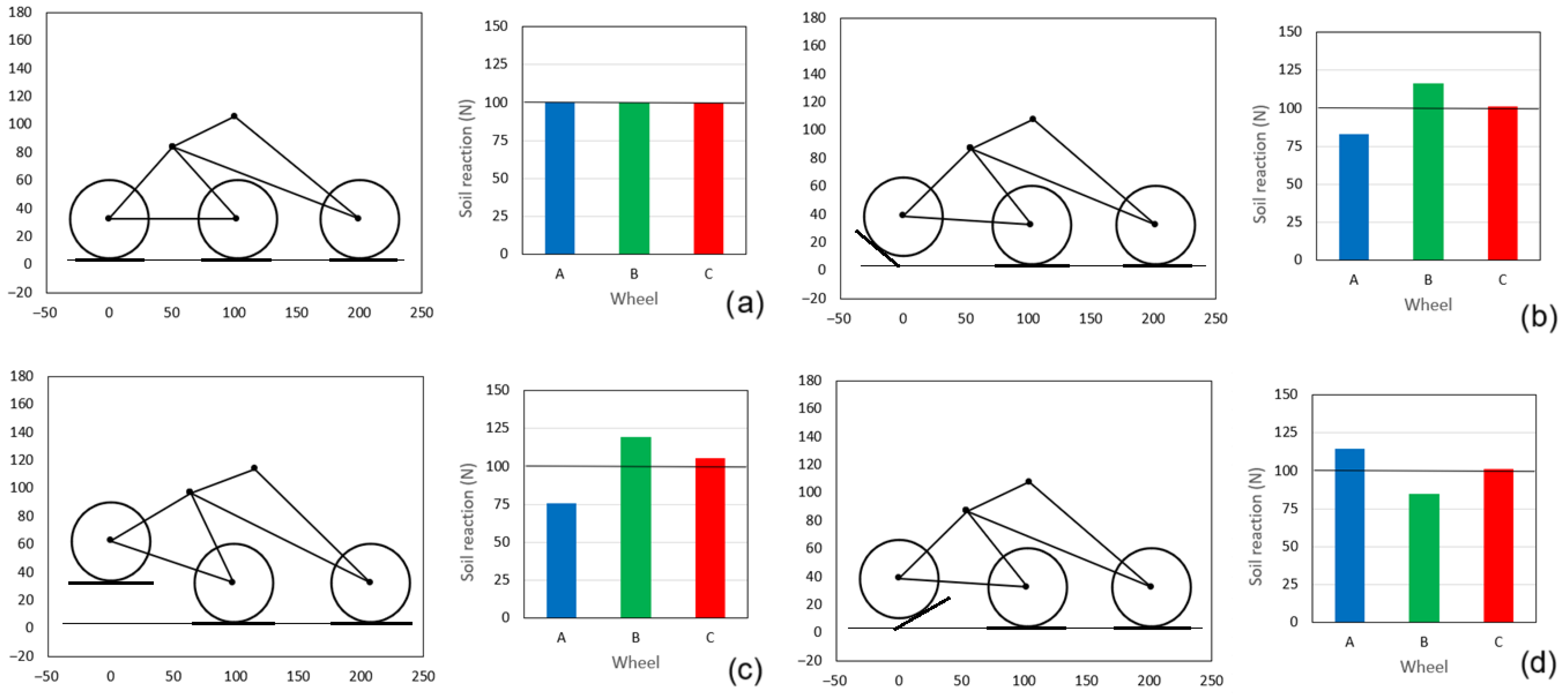
In Figure 12, some phases of overcoming a harmonic bump are reported, and for each phase, in

Table 4. Ground reaction forces at different contact points for Wheel A, considering λ = 100 mm, h = 30 mm.

	x (mm)	z (mm)	α (deg)	r cosα (mm)	zA (mm)	Ra	Rb	Rc	R*a	R*b	R*c
(a)	0	0	0	32.5	32.5	100	100	100	100	100	100
(b)	25.0	15	−43.3	23.6	38.6	83	116	101	85	109	101
(c)	50.0	30	0	23.6	62.6	76	119	105	76	119	105
(d)	75.0	15	+43.3	23.6	38.6	114	85	101	85	109	101

, the values of the main characteristic quantities are shown. The normalized vertical reactions of the soil (R_a, R_b, R_c) are compared with those calculated at the wheel axles (R*_a, R*_b, R*_c), which do not consider the horizontal displacement of the contact point due to the inclination of the ground. In the configurations (b) and (d), the reactions Ri and R*_i are equal. In particular, the following configurations were considered:

(a)

Wheel A is not yet engaged on the bump; all the wheels are at the same level on a horizontal surface, and the three reactions are equal; this condition is a reference for subsequent ones.

(b)

Ascent phase with mid-height contact (z = h/2 = 15 mm; α = −43°).

(c)

Contact on the crest of the wave (z = h = 30 mm; α = 0).

(d)

Descent phase with contact at half height (z = h/2 = 15 mm; α = +43°).

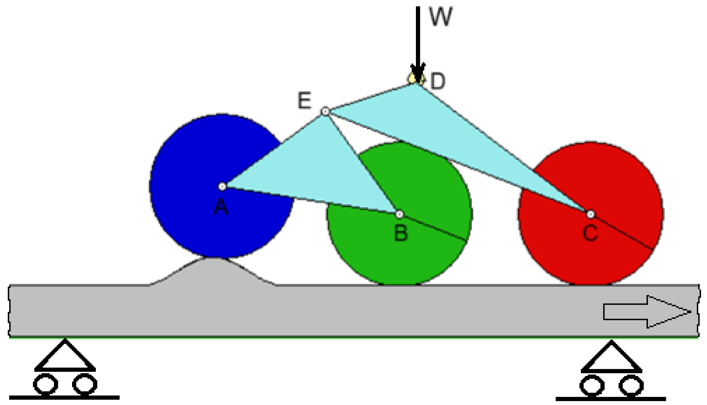
Ground reaction forces can also be evaluated by means of a multibody model represented in Figure 13. In this formulation, the rigid wheels are assumed to interact with a sliding rigid ground profile containing a harmonic bump; each wheel contacts the ground at a point that serves as its instant center of rotation. It is therefore assumed that friction at this point is sufficient to prevent any slipping. Passive resistances are disregarded, and the analysis focuses exclusively on the force generated by the bump opposing the rover’s forward progression. To this end, the ground is translated at a sufficiently low constant velocity (0.01 m/s) in the negative direction. The bump was chosen with a length of 80 mm and a height of 16 mm.

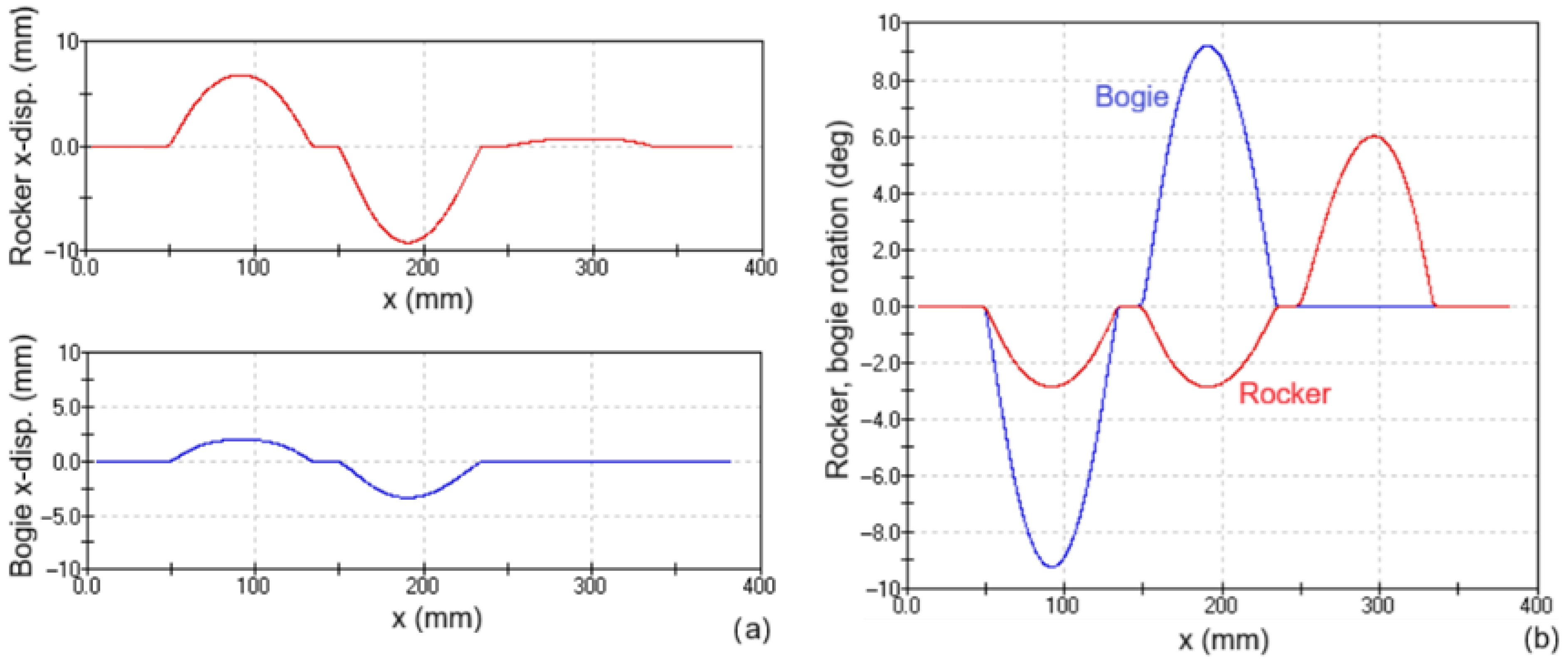
Figure 14 shows that, when the bump engages with each wheel, the two bodies first undergo a horizontal displacement, in the same direction as the motion of the bump and then in the opposite direction, until they return to the starting position, as shown by the diagrams in Figure 15a. Contact between the bump and wheel C results in zero horizontal displacement of the bogie and a small displacement of the rocker.

As shown in Figure 15b, the rotations of the rocker and the bogie exhibit distinct behaviors depending on which wheel crosses the bump. When wheel A encounters the bump, both the rocker and the bogie rotate clockwise (negative rotation). In contrast, when wheel B crosses the bump, the two bodies rotate in opposite directions. Finally, the bump encountered by wheel C induces only a counterclockwise rotation of the rocker.

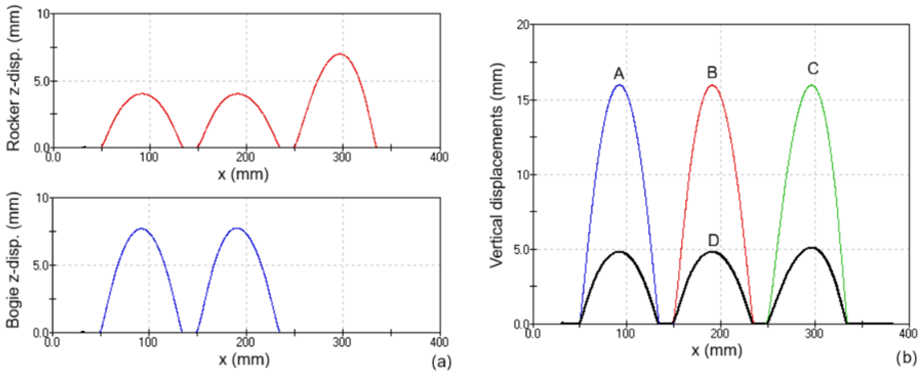
Figure 16a shows the vertical displacement of both bodies, while Figure 16b presents a comparison between the displacement of the wheels and that of point D, which represents the rover’s main body. The displacement of point D is approximately 3.2 times smaller than that of the wheels. All displacements are calculated with respect to the initial position, i.e., the configuration of the rover before encountering the bump.

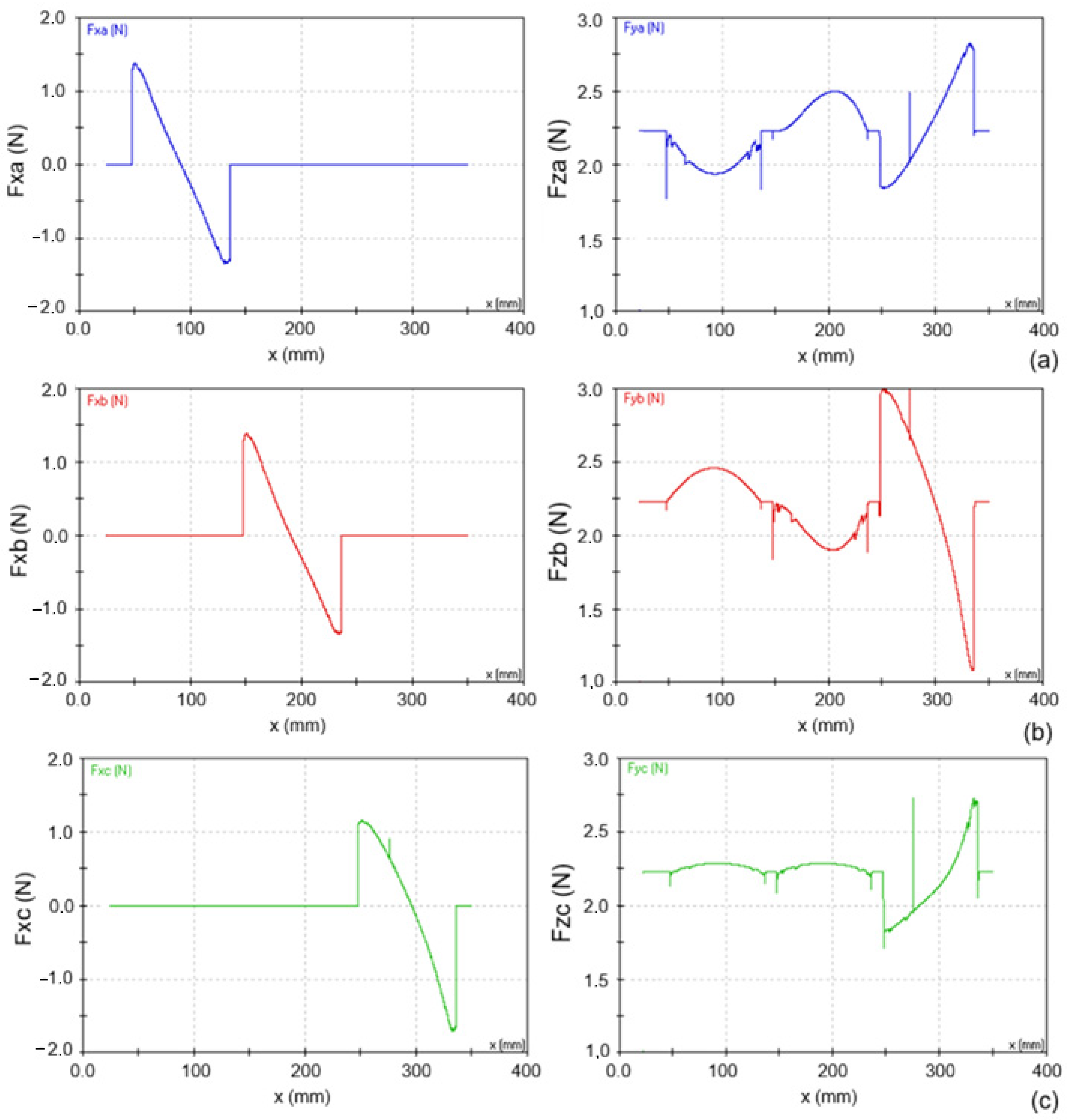
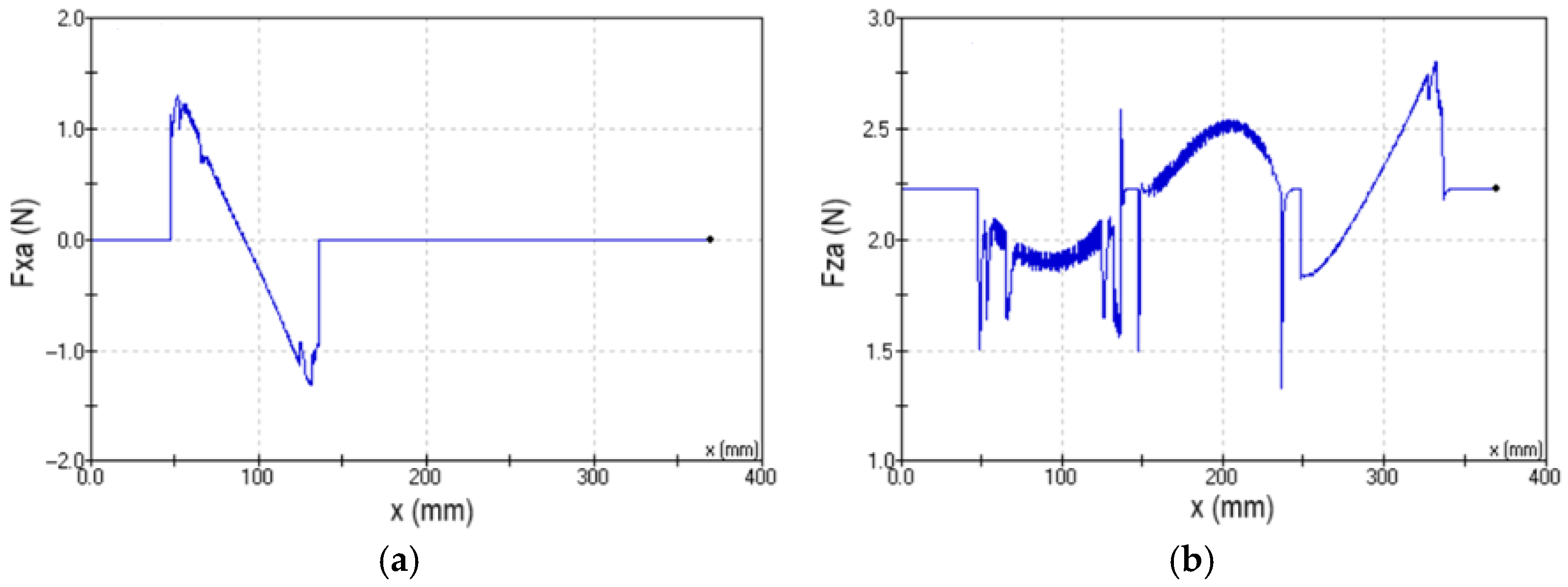
Figure 17 shows diagrams of the components of the soil-wheel contact forces obtained at a speed of 0.01 m/s. Before the rover engages with the bump, the three horizontal ground reactions are zero, and the vertical ones are equal.

When crossing the bump, the trend of horizontal actions is similar for the three wheels. Since the system is conservative, the area subtended by each curve in the ascent phase is equal to the negative area of the descent phase.

Regarding the vertical reactions, when wheel A engages with the bump, the clockwise rotation of the rocker causes wheel C to approach the line of action of the load W, acting at point D, while point E moves away from the same line. Consequently, the load on wheel C increases and the load on wheel E decreases. Due to the clockwise rotation of the bogie, the lower load in E is balanced to a greater extent by the wheel B which tends to move closer to the vertical line for E. The diagrams show an increase in loads in B and C and a reduction in load in A.

When wheel B engages with the bump, the opposite rotations of the rocker and bogie determine an increase in load in C; the load acting in E loads wheel A more.

Finally, when wheel C is on the bump, the counterclockwise rotation of the rocker results in less load on wheel C; in the ascent phase, the point of contact is closer to E than the center of the wheel; in the descent phase, the opposite occurs, and this explains the increasing trend of the corresponding reaction. The bogie does not rotate, and the load E is equally balanced by wheels A and B.

At the beginning and at the end of the contact of each wheel with the bump, a peak in force is noted due to the initial acceleration imposed by the bump on the wheel.

As the speed increases, due to numerical problems, the contact forces begin to have more irregular trends, making it more difficult to analyze dynamic behavior. In Figure 18, the trend of the contact force of wheel A is shown, performed at a speed of 0.1 m/s. In addition to the peaks due to the contact skipping, the graph is bouncing and with intermediate peaks throughout the harmonic profile. A more precise analysis would require, each time, to redefine the geometry of the bump profile with a more extreme discretization.

5. Axle Motion of Wheel A over a Harmonic Bump

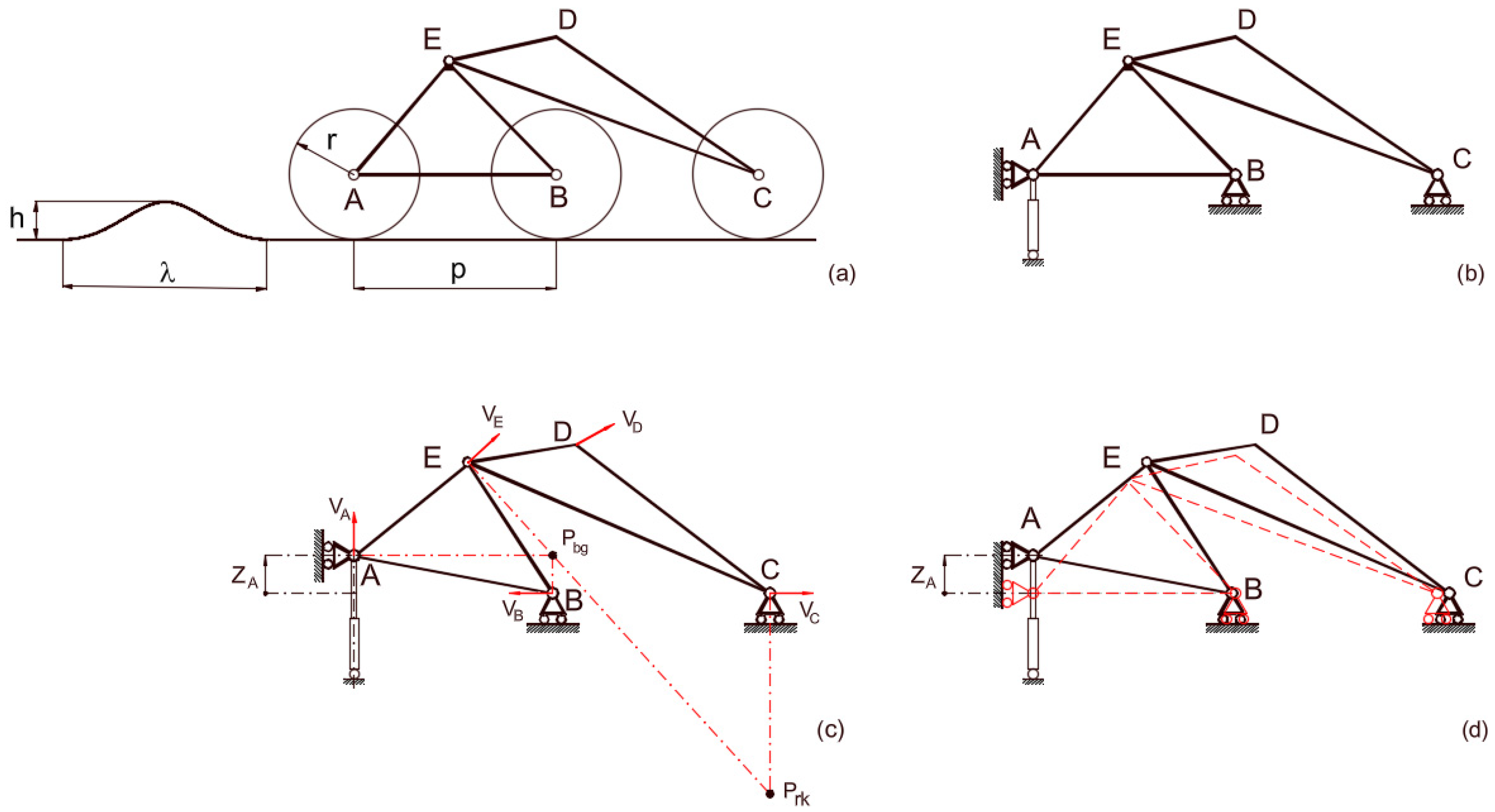
Figure 19 shows that, when wheel A engages with the bump, its axis undergoes a vertical shift; consequently, wheels B and C undergo horizontal translation. This situation can be schematized by constraining the axle of wheel A with a vertical guide and the axles of wheels B and C with horizontal guides (Figure 19b). The 2D model is constituted by an articulated single-degree-of-freedom system, consisting of two rigid bodies (rocker and bogie) connected to each other by a revolute joint and constrained to the frame by three sliding joints arranged at the wheel axes. The model does not consider friction between the wheel and the ground. By imposing a vertical motion on the axis of the wheel A, described by Equation (7) or Equation (13) (by means of the actuator schematized in Figure 19b), the rocker and the bogie undergo a clockwise rotation around the instant centers of rotation shown in Figure 19c in which the velocity directions, relating to the lifting phase of wheel A, are reported. These rotations involve a positive horizontal displacement of wheel B and a displacement of the opposite sign of wheel C (analogously to the case of Figure 15a). The masses concentrated at points A, B, C, and D accelerate, and the corresponding vertical inertia forces are balanced by the ground constraint reactions.

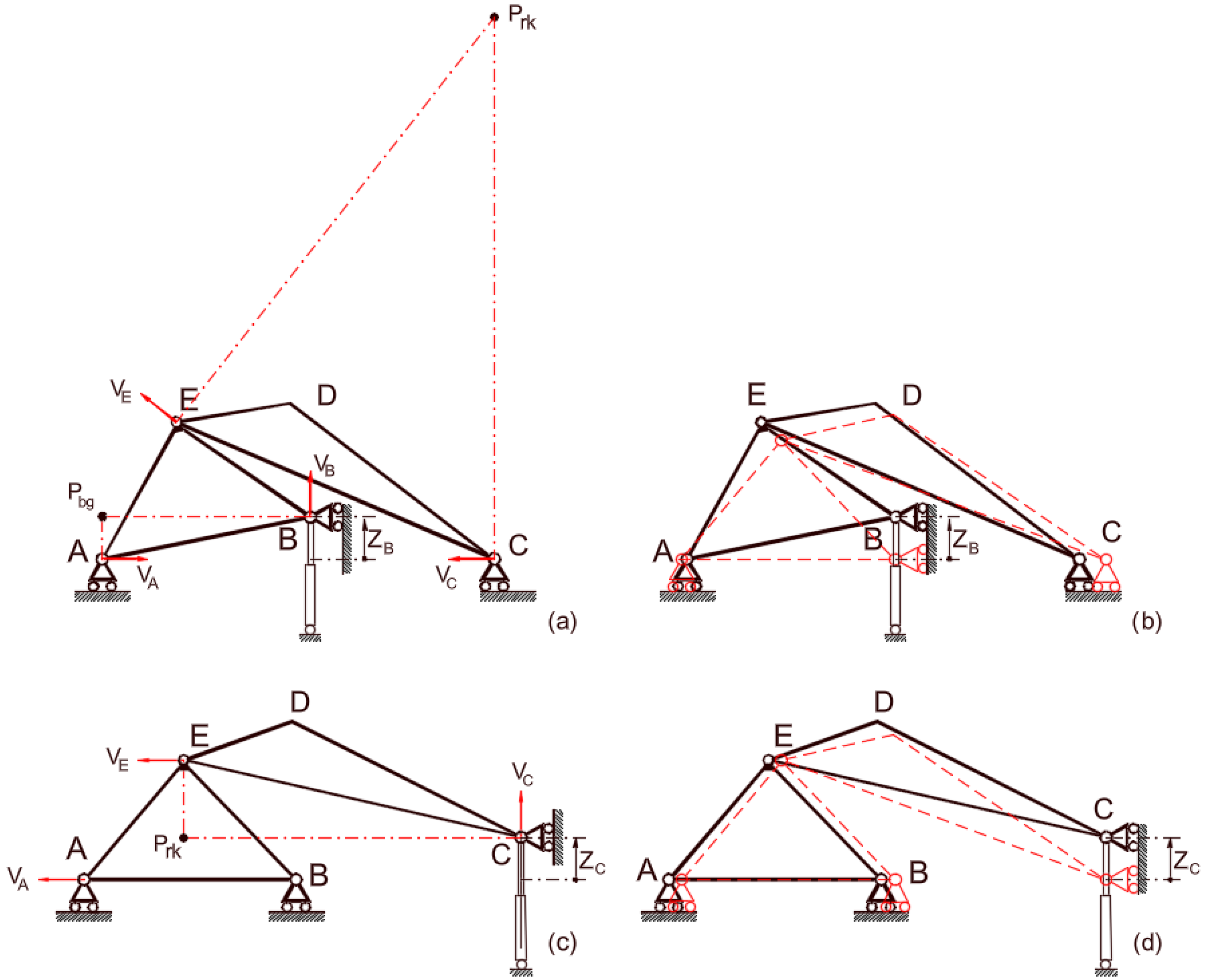
Being the wavelength of the obstacle shorter than the wheelbase of the bogie (λ < p), the wheels pass the bump in succession, and therefore only one wheel at a time is engaged with the bump. Figure 20 shows the instant centers of rotation and the configuration assumed by the rover when wheels B and C interact with the obstacle.

Therefore, once the forward speed and the characteristics of the bump ($h, \lambda )$ vary, it is possible to define the trend of the vertical reactions at the wheel centers. If the wheel radius is small compared to the wheelbase, the obtained values can be regarded as a good approximation of the ground reactions on the wheels.

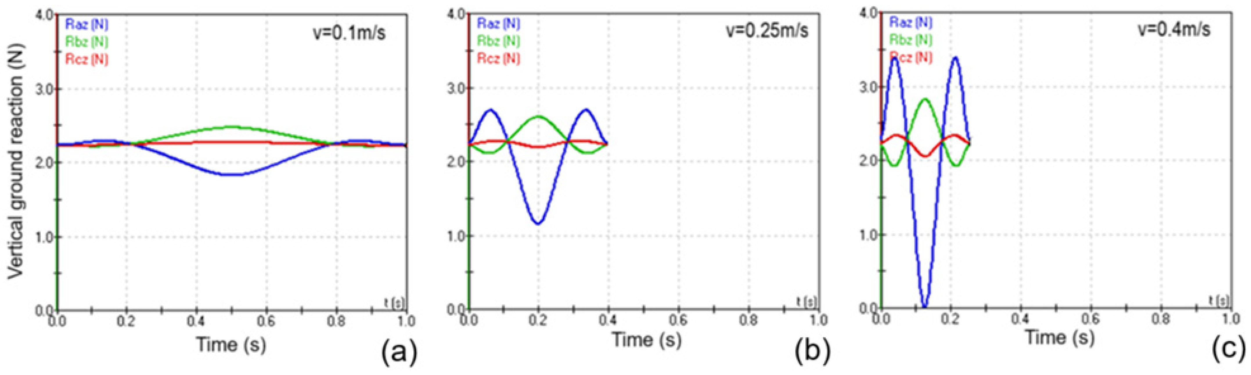
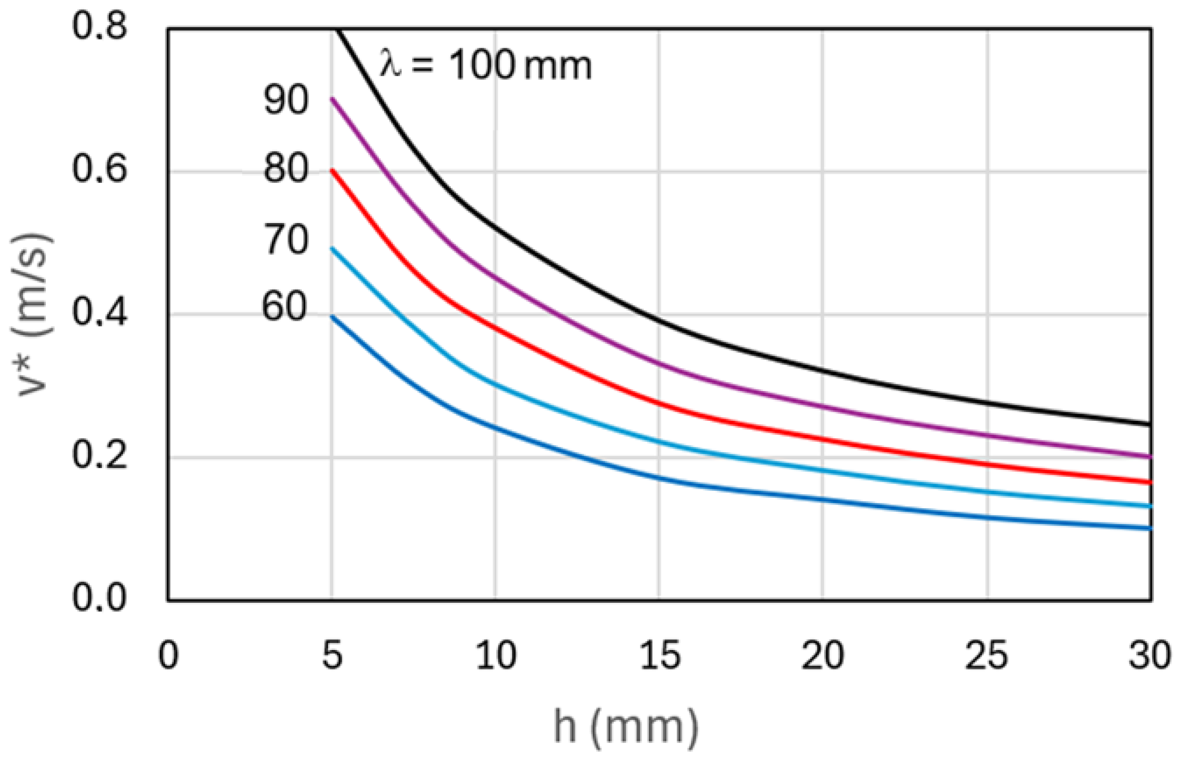
In Figure 21 the three vertical reactions are shown for three different values of the forward speed v and therefore of the fundamental rotating frequency of the forced motion (${\omega }_s=2\pi v/\lambda$). The diagram shows that at the speed of 0.4 m/s the reaction of wheel A is zero when the wheel reaches the crest of the bump. This value represents the threshold speed at which wheel A loses contact with the ground, and it is referred to as the first lift-off speed. Beyond this value, the wheel tends to lift off the ground and then land, generating high stresses due to the subsequent impact. As the height of the bump varies, it is possible to derive the threshold speed for different wavelength values. Figure 22 shows a map of the threshold speed confirming the expected trend; for a fixed height, increasing the wavelength allows the obstacle to be traversed at a higher speed. The threshold value was defined with a tolerance of 0.01 m/s.

In bump obstacles, the wavelength is smaller than the wheelbase; this condition has influenced the wavelength values. For the height of the bump, a maximum height equal to the wheel radius was considered.

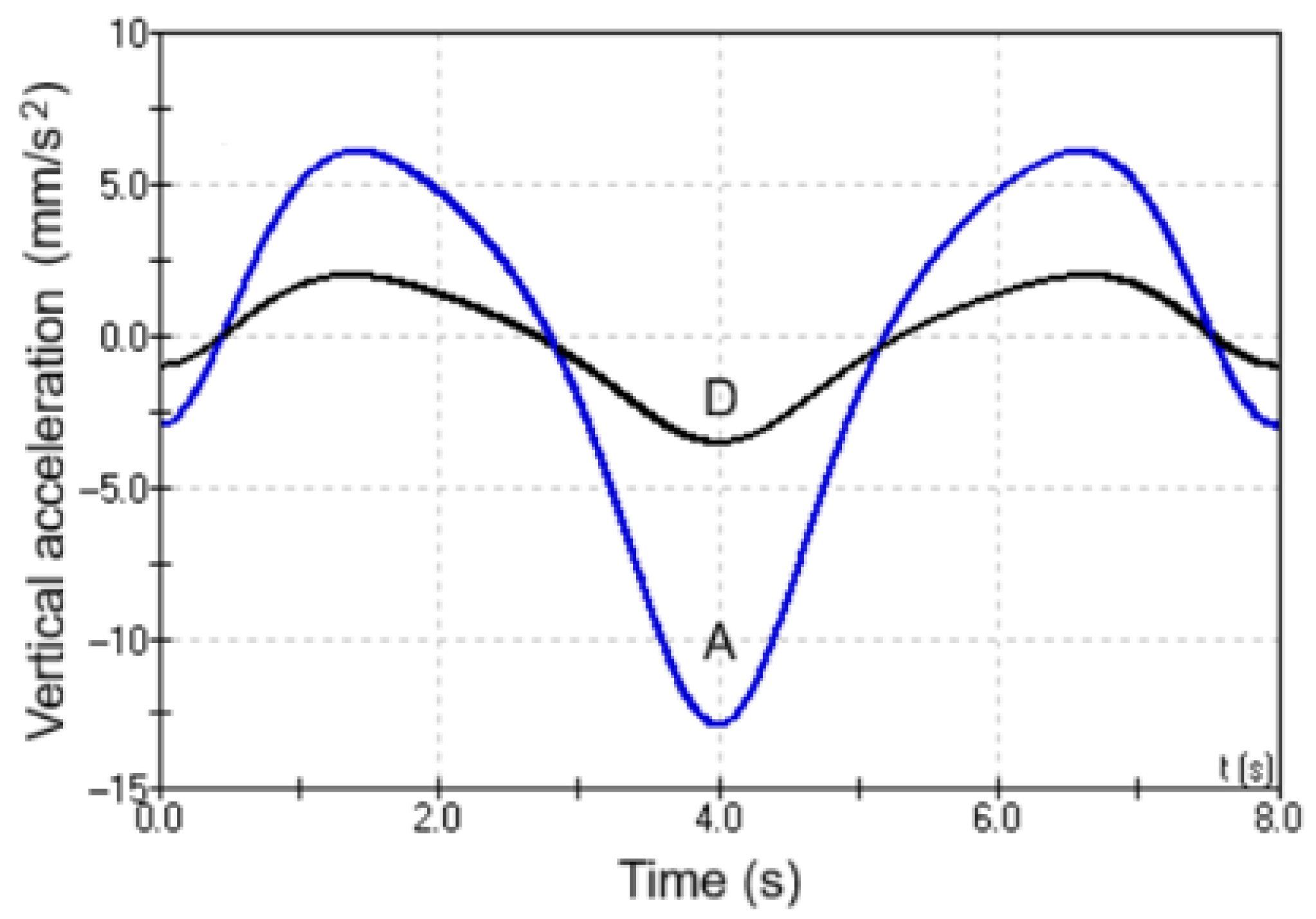
All other quantities being equal, as the bump height (h) increases, two concomitant effects arise that promote wheel detachment from the bump. First, the increased vertical displacement of the wheel leads to a greater reduction in static load. Figure 23 shows the second effect, consisting of the upward inertial force due to the more pronounced negative acceleration of the wheel center.

6. Axle Motion of Wheel B and C over a Harmonic Bump

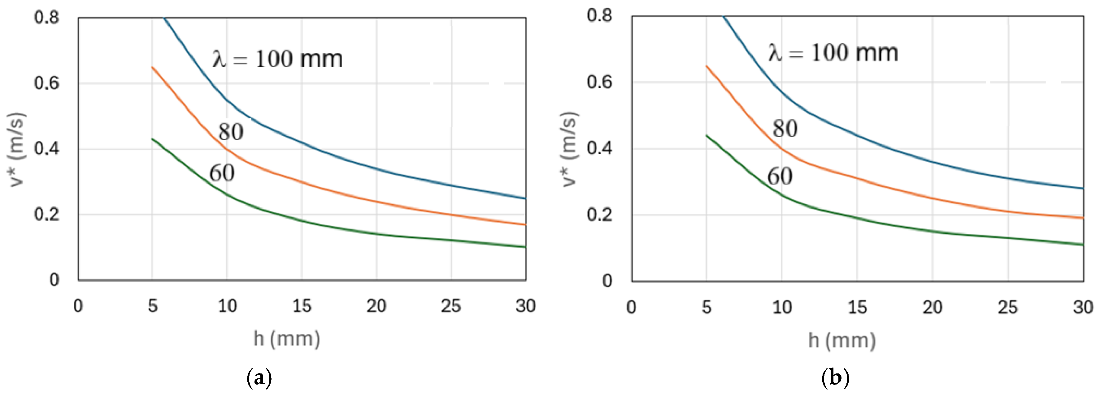
The procedure described has been repeated by imposing the vertical motion, provided by Equation (13), on wheels B and C to determine the first lift-off speed. Figure 24 reports the corresponding threshold maps.

To actuate wheel B, it must be considered that in the starting configuration, the mechanism presents a kinematic singularity, as shown in Figure 19, if the points A, B, and C are aligned. For this reason, the wheel-first lift-off speeds were carried out considering a starting configuration in which point B is slightly higher than points A and B.

Finally, actuating wheel C along the vertical direction and constraining A and B to slide horizontally, the rocker behaves as an elliptical trammel mechanism; points B and C of the rocker move in mutually orthogonal directions.

The simulation results show that both static and dynamic loads undergo similar variations for the three wheels.

Table 5. Normalized vertical reactions for three configurations of the rover.

	h1 (mm)	h2 (mm)	h3 (mm)	Ra (N)	Rb (N)	Rc (N)
(a)	15	0	0	88	109	103
(b)	0	15	0	109	88	103
(c)	0	0	15	103	103	94

shows the ground reactions on the wheels as each one approaches the crest of the bump.

The maps in Figure 24 also show slight variations between the values of the wheel-first lift-off speeds for the three wheels. Therefore, it is sufficient to check that one of the wheels travels at a speed lower than the lift-off threshold. In this regard, it should be noted that, for the values of h of interest, the curves can be approximated with exponential functions:

$$v^{*}=k h^b$$

(16)

in which k determines the value of the first detachment velocity for h unitary and the exponent b controls the speed with which the curve decreases. By interpolating the curves with an exponential function (16), k and b can be expressed with the following linear functions of λ:

b(λ) = −0.00248 λ + 0.924; k(λ) = 0.0253 λ − 0.095

(17)

In these expressions, λ is expressed in mm, b is dimensionless, $h$ is expressed in m, and $v^{*}$ is expressed in m/s. Therefore, if the height (h) and the wavelength (λ) of the obstacle can be estimated (for example, with vision sensors), the corresponding first detachment velocity can be derived.

7. Experimental Tests

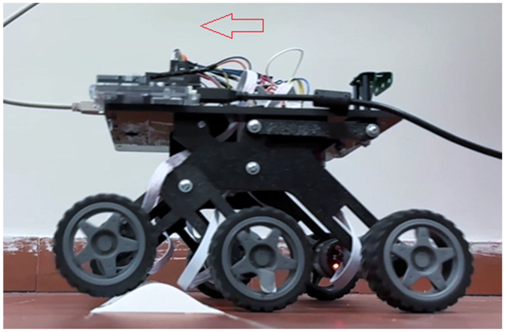
Preliminary experimental tests were carried out using a Runt Rover™ bogie platform [31], represented in Figure 25, manufactured in ABS (acrylonitrile-butadiene-styrene). The geometric specifications of the rover are listed in Table 1.

The rover is equipped with six independently driven wheels, each with a diameter of 65 mm and a width of 25 mm. Wheel actuation is provided by six identical 12 V DC motors mounted on the wheel axles, each coupled to a 30:1 gearbox. The motors deliver a rated torque of 350 Nmm at a nominal speed of 250 RPM, ensuring adequate traction and mobility for the platform.

Table 6. Technical specifications of the equipment adopted for the tests.

Equipment	Specification
control board	Arduino UNO Wi-Fi Rev2 (Arduino S.r.l./Arduino AG, Ivrea, Italy)
control board	Adafruit Motor Shields v2.3, (Adafruit Industries, Brooklyn, NY, USA)
IMU	LSM6DS3TR (integrated in Arduino UNO)
motors	12 V DC with 30:1 gearbox; torque of 350 Nmm @ 250 RPM,
Video camera	iPhone 16, 48 MP; 240 fps (Apple Inc., Cupertino, CA, USA)

shows the equipment used for experimental tests. The rover is equipped with an Arduino UNO Wi-Fi Rev2 control board [32] flanked by two Adafruit Motor Shields v2.3 [33], each connected to the three motors on one side of the rover. These boards were used because the current supplied by Arduino is not sufficient to directly power all the motors. The Arduino board is equipped with an integrated LSM6DS3TR [34] IMU sensor that provides measurements of the angular velocities and accelerations of the rover’s body. The bump profile used for the experimental tests features a wavelength of 80 mm and a height of 16 mm.

The tests were conducted at various speeds of the rover. For each test, the rover motion was recorded using a video camera in slow motion mode, while signals coming from the IMU and from the wheel encoders were simultaneously acquired. The first lift-off speed was detected by analyzing the video frames.

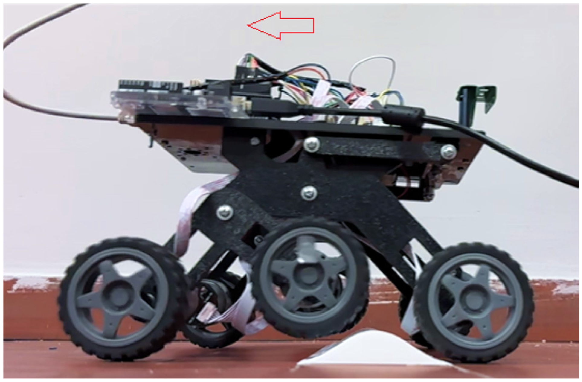
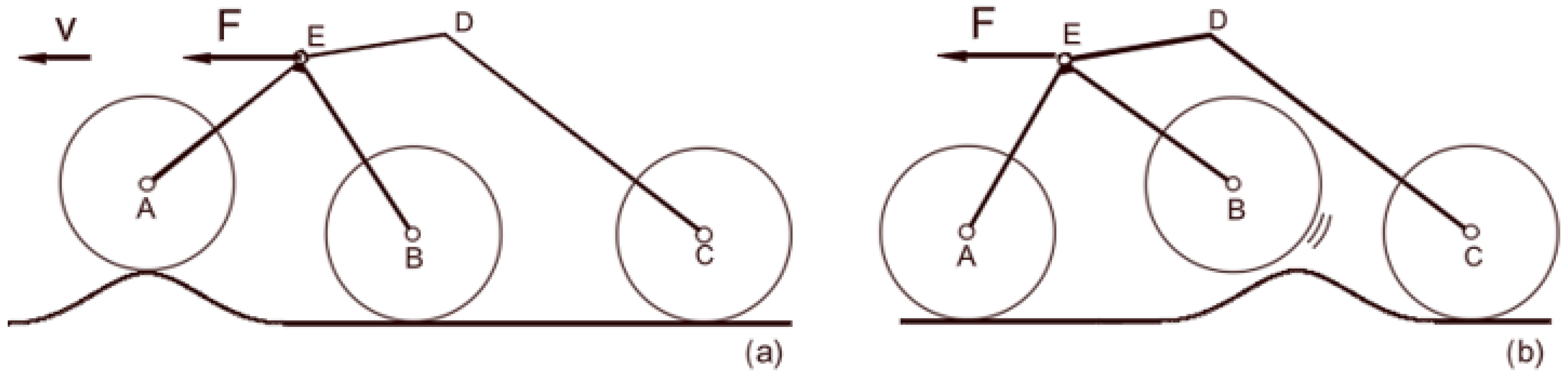
Results show that the lift-off speed on a profile with L = 80 mm and h = 16 mm is approximately 0.3 m/s, which agrees with theoretical predictions. However, it was observed that the lift-off occurs earlier on the middle wheels, as shown in the photograph in Figure 26 obtained at a speed of 0.4 m/s. This can be explained by considering that, during the bump ascent phase, the rover’s body experiences a deceleration. Consequently, with reference to Figure 27, the body horizontal inertia force transmitted at point E, produces a moment that alters the normal load distribution between the two bogie wheels, increasing the load on the front wheel while reducing it on the rear wheel. This variation in load influences how the first two wheels traverse the bump. When the front wheel is on the crest (Figure 27a), the moment tends to press it against the bump, whereas when the intermediate wheel is on the crest (Figure 27b), the moment tends to lift it. Similarly, when the rover moves in the opposite direction (rocker forward), the first wheel to lift off the ground is wheel A.

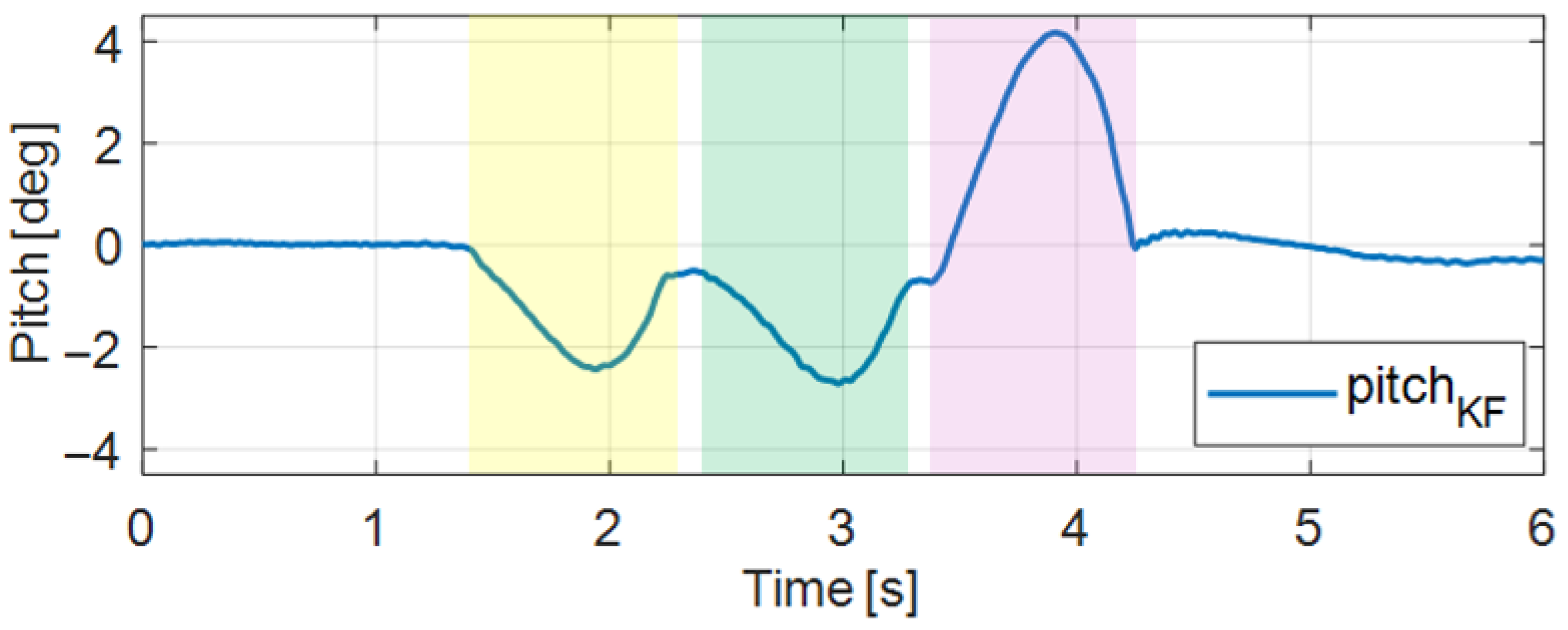
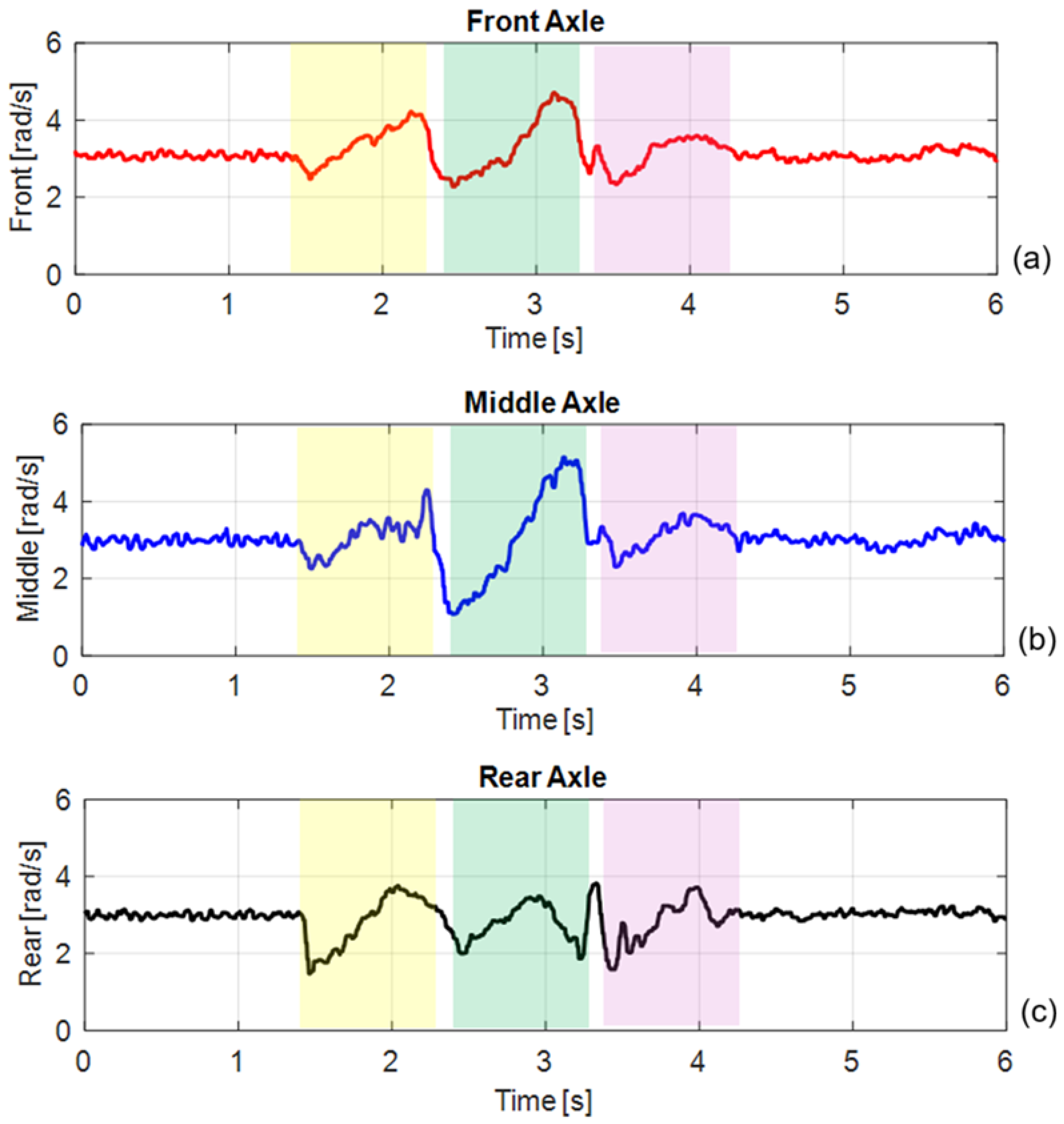
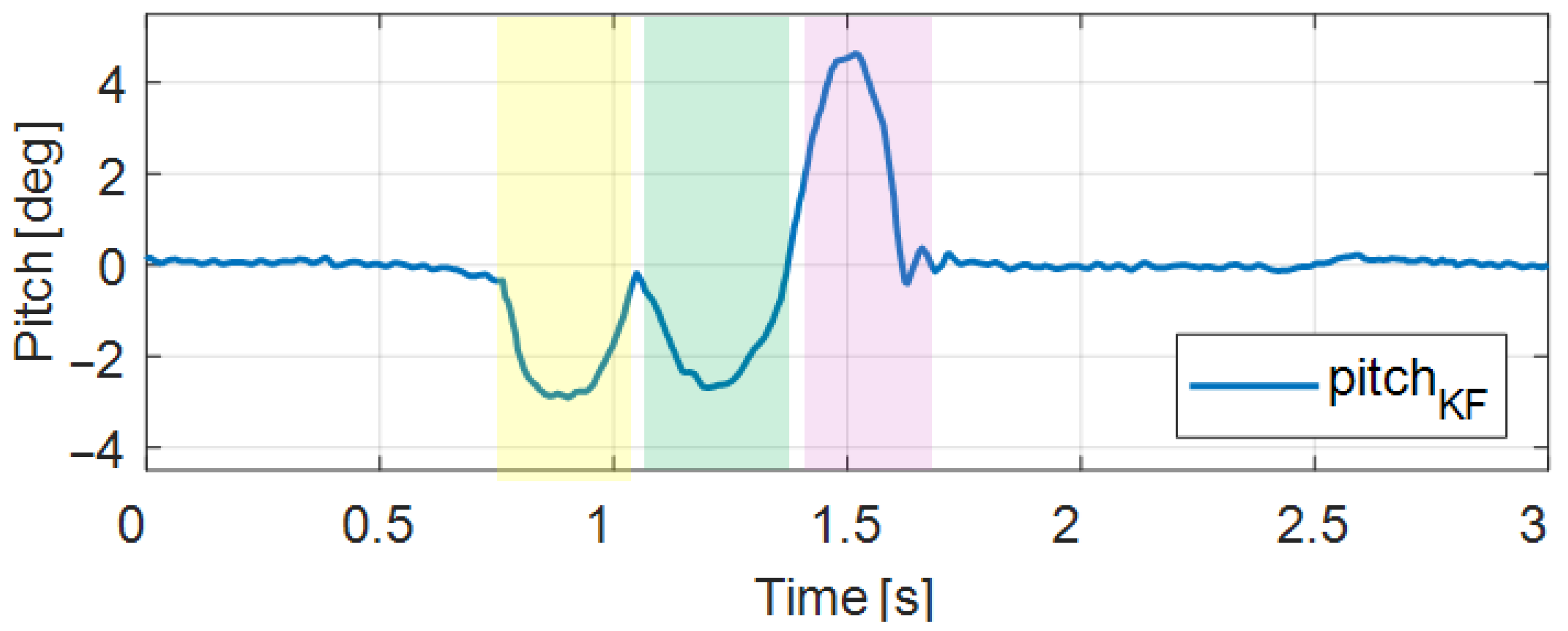
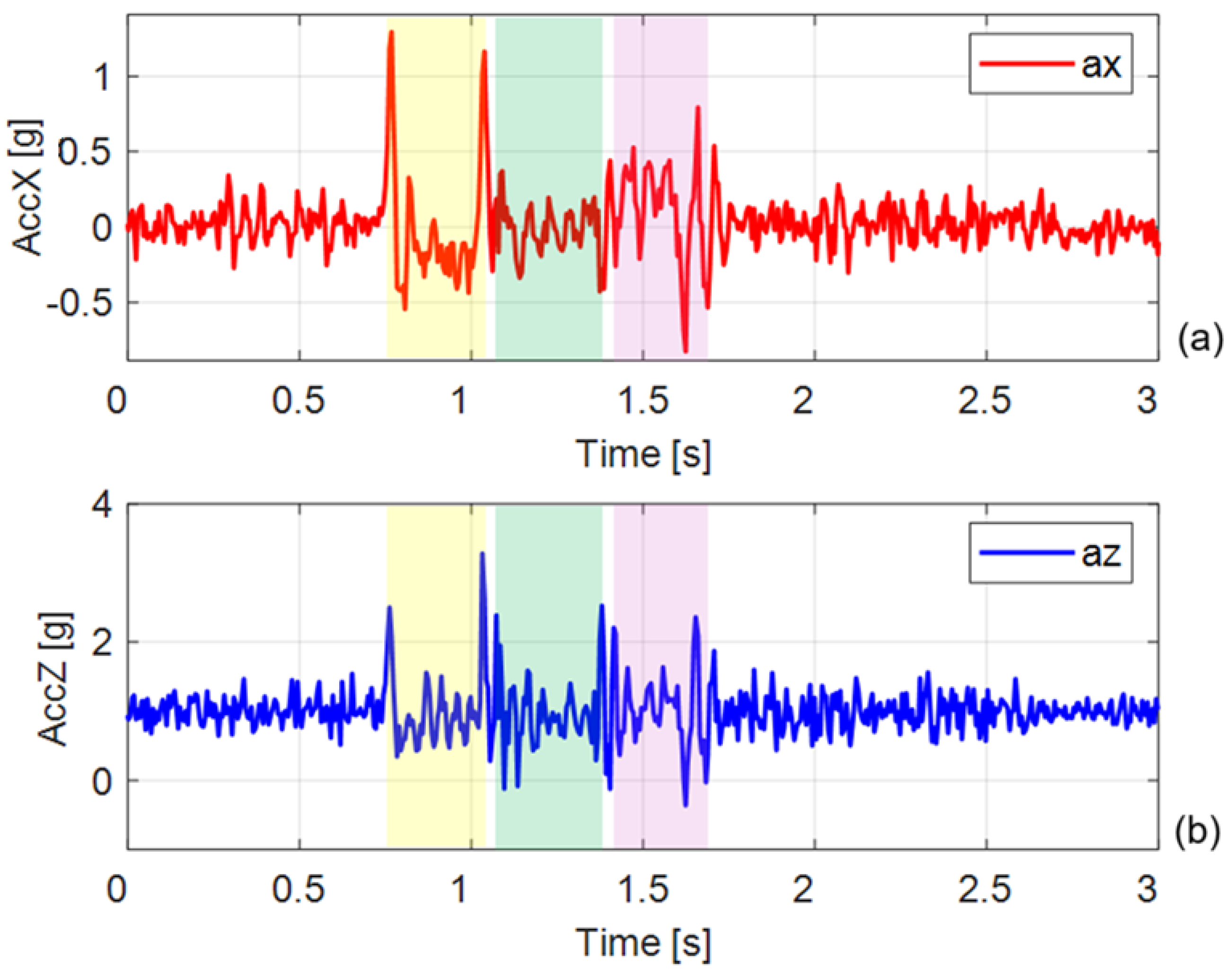
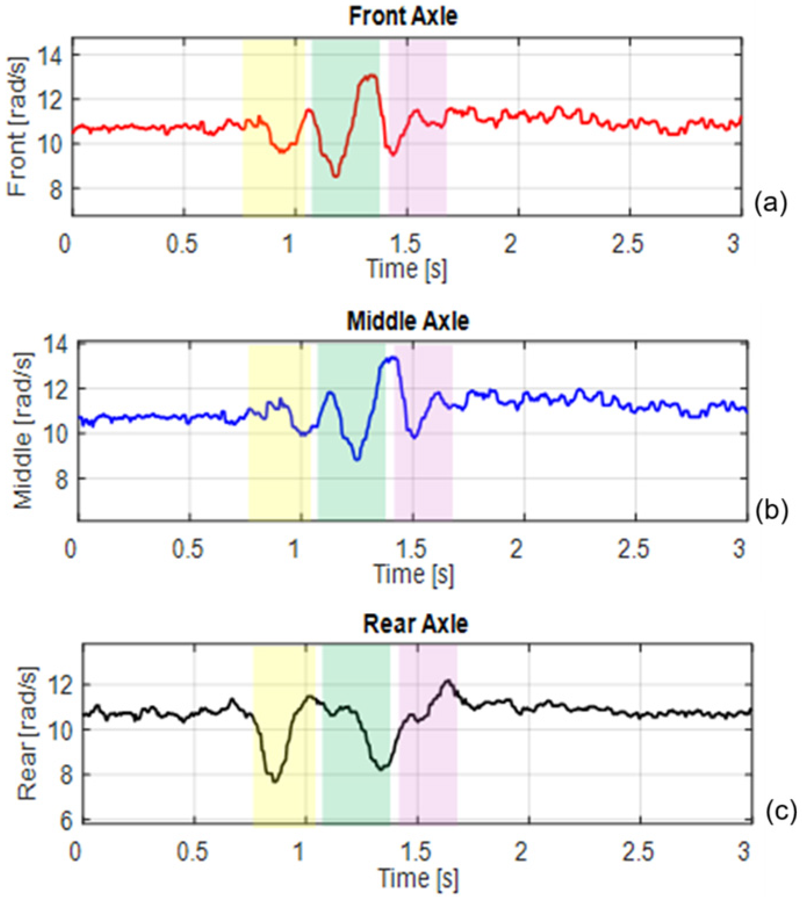
As an example, the signals detected by assigning the rover a speed of 0.1 m/s, which is lower than that of the first lift-off speed, are reported. Figure 28, Figure 29 and Figure 30 show the gyroscopic, accelerometric and encoder signals of the wheels of the same side, respectively.

The gyroscopic sensor shows the pitch rotation of the body (in Figure 28) which (as described in the diagram in Figure 15b), has two consecutive clockwise rotations, due to the crossing of wheels A and B on the bump, which lead to a raising of the point E; the last rotation of the body is due to the crossing of the C wheel which involves an counterclockwise rotation of the rocker (equal to that of the body).

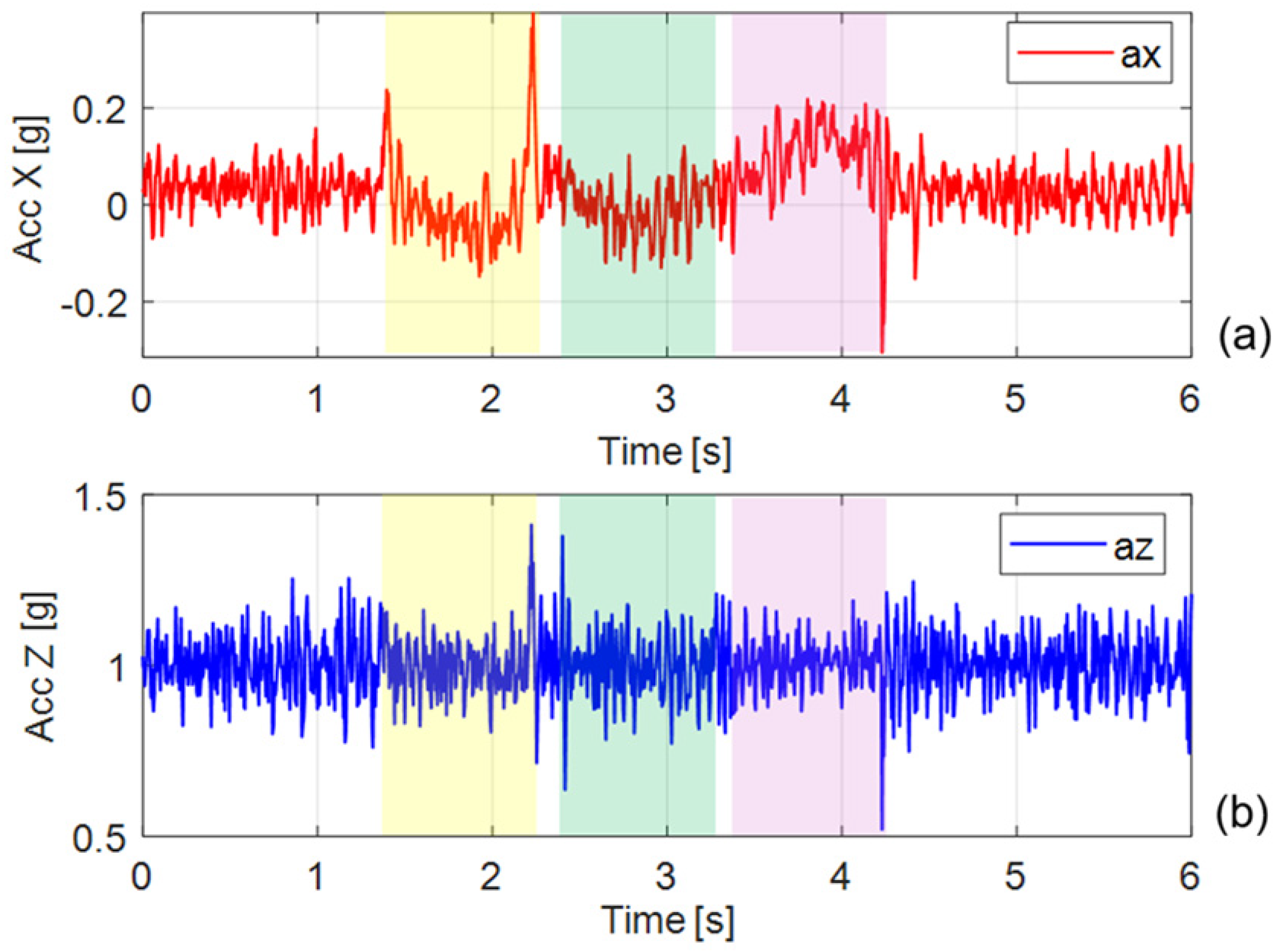
The accelerometer data indicate a longitudinal deceleration when the bogie wheels encounter the bump, followed by an acceleration as the rocker wheel climbs over it, how reported in Figure 29a. When the first two wheels cross the bump, the clockwise rotation of the body causes a longitudinal deceleration of the body; the opposite occurs when the rear wheel climbs the bump. Regarding vertical acceleration, Figure 29b highlights peaks of greater amplitude are noted when the wheels begin or complete the climb of the bump.

The encoder signals (Figure 30) show that the wheels undergo a sudden reduction in speed every time one of them comes into contact with the bump; after that, the speeds increase until they exceed the initial value in the descent phase from the bump. The diagrams show a spike when the rear wheel encounters the bump, which may indicate wheel slip caused by the sudden reduction in wheel load.

The following tests were carried out at a speed of 0.35 m/s, for which the video frames clearly show the detachment of the central wheel from the bump (as already shown in Figure 25). The body rotations (Figure 31), the accelerations (Figure 32), and the rotation wheel speeds (Figure 33) reach higher values compared to the previous case. The combination of negative longitudinal acceleration with positive vertical acceleration during the second phase of the intermediate wheel’s contact with the bump results in the lift-off of the intermediate wheel.

8. Conclusions

This study addressed the dynamics of a rocker–bogie rover traversing periodic obstacles modeled as harmonic bumps. The kinematics of the system were described, and a simplified model was proposed to determine the wheel-first lift-off speed. The subsequent dynamic analysis focused on identifying the forward velocities beyond which a wheel loses ground contact. The results demonstrated how these threshold speeds are influenced by the geometric parameters of the obstacle.

The experimental tests presented in this paper aim to illustrate the dynamic phenomenon under investigation. A comprehensive large-scale experimental campaign, involving bumps with different profiles and considering variations in rover mass and mass distribution, is planned for future studies. The simplified model proposed to estimate the first lift-off speed can be considered valid under the assumptions that the rover’s trajectory is orthogonal to the bump and that the system can be represented in two dimensions.

The investigation is conceived as a preparatory step towards the integration of perception and control. If the rover is equipped with a vision system capable of detecting and characterizing obstacles, the deductions presented here can support autonomous decision-making. Depending on the estimated obstacle geometry, the rover may either replan its path to bypass it or choose to traverse it. In the latter case, the results of this study provide the maximum admissible traversal velocity that ensures ground contact and traction are maintained.

Overall, the proposed framework helps bridge the gap between the mechanical modeling of suspension systems and autonomous navigation strategies, offering a foundation for the development of robotic platforms capable of safe and efficient operation in irregular environments.

References

1. Bickler, D.B. Roving over Mars. Mech. Eng. 1998, 120, 74–77. [Google Scholar] [CrossRef]
2. Eisen, H.J.; Buck, C.W.; Gillis-Smith, G.R.; Umland, J.W. Mechanical Design of the Mars Pathfinder Mission. In Proceedings of the 7th European Space Mechanisms and Tribology Symposium, Noordwijk, The Netherlands, 1–3 October 1997. [Google Scholar]
3. Harrington, B.D.; Voorhees, C. The Challenges of Designing the Rocker-Bogie Suspension for the Mars Exploration Rover. In Proceedings of the 37th Aerospace Mechanisms Symposium, Galveston, TX, USA, 19–21 May 2004; Johnson Space Center: Houston, TX, USA, 2004. [Google Scholar]
4. Lindemann, R.A.; Voorhees, C.J. Mars Exploration Rover Mobility Assembly Design, Test and Performance. In Proceedings of the 2005 IEEE International Conference on Systems, Man and Cybernetics, Waikoloa, HI, USA, 10–12 October 2005; Volume 1, pp. 450–455. [Google Scholar] [CrossRef]
5. Bickler, D. The Mars Rover Mobility System. JPL Open Repository. 1997. Available online: https://dataverse.jpl.nasa.gov/file.xhtml?fileId=25641&version=1.1 (accessed on 15 September 2025).
6. Cosenza, C.; Malfi, P.; Nicolella, A.; Niola, V.; Pagano, S.; Savino, S.; Spirto, M. Mechanical Models of Six-Wheeled Rocker-Bogie Rovers for the Study of Obstacle Overcoming. Int. J. Mech. Control 2023, 24, 75–88. [Google Scholar]
7. Cosenza, C.; Niola, V.; Pagano, S.; Savino, S. Theoretical Study on a Modified Rocker-Bogie Suspension for Robotic Rovers. Robotica 2023, 41, 2915–2940. [Google Scholar] [CrossRef]
8. Li, J.; He, J.; Xing, Y.; Gao, F. Dimensional Optimization of Rocker-Bogie Suspension for Planetary Rover Based on Kinetostatics and Terramechanics. Proc. IMechE Part C J. Mech. Eng. Sci. 2021, 236, 246–262. [Google Scholar] [CrossRef]
9. Di Massa, G.; Pagano, S.; Rocca, E.; Savino, S. Six-Wheeled Mobile Manipulator for Brush Cleaning in Difficult Areas: Stability Analysis and Grip Condition Estimation. Machines 2025, 13, 359. [Google Scholar] [CrossRef]
10. Rathod, V.; Mokashi, P.; Thakare, P.; Yadav, D. Design of Rocker-Bogie Mechanism for Application in Agriculture. Int. J. Robot. Autom. 2022, 8, 13–17. [Google Scholar]
11. Sandbhor, R.; Kachale, S.; Bhosale, A.; Gaikwad, A.; Kshirsagar, K.; Sharma, P. Design and Development of an Autonomous Rover Application Using a Rocker-Bogie Mechanism in Agriculture. Int. J. Adv. Res. Sci. Commun. Technol. 2024, 4, 562–572. [Google Scholar] [CrossRef]
12. Llontop, L.; Ramos, N.M. Optimization of Rocker–Bogie Suspension System for Robustness Improvement of Autonomous Rover by Numerical Simulations for Irregular Surfaces in Precision Agriculture. Eng. Proc. 2025, 83, 20. [Google Scholar] [CrossRef]
13. Shanmugasundar, G.; Adithya, S.; Nagappan, V.; Jagadeeshwar, P.; Bhaskar, M. Design and Fabrication of Stair Climbing Wheelchair with Rocker-Bogie Mechanism. J. Eng. 2018, 8, 7–11. [Google Scholar]
14. Arora, A.; Sivan, G.S.S.; Irani, J.; Ahluwalia, M.S.; Kumar, D. Design of Rocker-Bogie for Military Applications. In Proceedings of the International Conference on Advanced Materials, Energy and Environmental Sustainability, Dehradun, India, 14–15 December 2018. [Google Scholar]
15. Rajath, S.; Shivakumar, N.; Pradhan, K.S. Rovers with Rocker-Bogie Mechanisms: A Review of Progress and Innovations in Design, Manufacturing, and Control. Proc. Inst. Mech. Eng. Part C J. Mech. Eng. Sci. 2024, 238, 6560–6583. [Google Scholar] [CrossRef]
16. Nayar, H.; Kim, J.; Chamberlain-Simon, B.; Carpenter, K.; Hans, M.; Boettcher, A.; Bittner, B. Design Optimization of a Lightweight Rocker–Bogie Rover for Ocean Worlds Applications. Int. J. Adv. Robot. Syst. 2019, 16, 1729881419885696. [Google Scholar] [CrossRef]
17. Ellery, A. Planetary Rovers—Robotic Exploration of the Solar System; Springer: Berlin/Heidelberg, Germany, 2016; ISBN 978-3-642-03258-5. [Google Scholar] [CrossRef]
18. Oroko, J.A.; Nyakoe, G.N. Obstacle Avoidance and Path Planning Schemes for Autonomous Navigation of a Mobile Robot: A Review. In Proceedings of the Sustainable Research and Innovation Conference, Nairobi, Kenya, 20–24 June 2022; pp. 314–318. [Google Scholar]
19. Skoczeń, M.; Ochman, M.; Spyra, K.; Nikodem, M.; Krata, D.; Panek, M.; Pawłowski, A. Obstacle Detection System for Agricultural Mobile Robot Application Using RGB-D Cameras. Sensors 2021, 21, 5292. [Google Scholar] [CrossRef] [PubMed]
20. Song, K.T.; Chiu, Y.H.; Kang, L.R.; Song, S.H.; Yang, C.A.; Lu, P.C.; Ou, S.Q. Navigation Control Design of a Mobile Robot by Integrating Obstacle Avoidance and LiDAR SLAM. In Proceedings of the 2018 IEEE International Conference on Systems, Man, and Cybernetics (SMC), Miyazaki, Japan, 7–10 October 2018; pp. 1833–1838. [Google Scholar]
21. Rostami, S.M.H.; Sangaiah, A.K.; Wang, J.; Liu, X. Obstacle Avoidance of Mobile Robots Using Modified Artificial Potential Field Algorithm. EURASIP J. Wirel. Commun. Netw. 2019, 2019, 1–19. [Google Scholar] [CrossRef]
22. Park, J.W.; Kwak, H.J.; Kang, Y.C.; Kim, D.W. Advanced Fuzzy Potential Field Method for Mobile Robot Obstacle Avoidance. Comput. Intell. Neurosci. 2016, 2016, 6047906. [Google Scholar] [CrossRef] [PubMed]
23. Zheng, W.; Wang, H.B.; Zhang, Z.M.; Li, N.; Yin, P.H. Multi-Layer Feed-Forward Neural Network Deep Learning Control with Hybrid Position and Virtual-Force Algorithm for Mobile Robot Obstacle Avoidance. Int. J. Control Autom. Syst. 2019, 17, 1007–1018. [Google Scholar] [CrossRef]
24. Ribeiro, T.; Gonçalves, F.; Garcia, I.; Lopes, G.; Ribeiro, A.F. Q-learning for Autonomous Mobile Robot Obstacle Avoidance. In Proceedings of the 2019 IEEE International Conference on Autonomous Robot Systems and Competitions (ICARSC), Vila Real, Portugal, 26–27 April 2019; IEEE: New York, NY, USA, 2019; pp. 1–7. [Google Scholar]
25. Tanimoto, T.; Shinohara, K.; Yoshinada, H. Research on Effective Teleoperation of Construction Machinery Fusing Manual and Automatic Operation. Robomech J. 2017, 4, 14. [Google Scholar] [CrossRef]
26. Mepani, M.; Guha, A. Study of the Step Climbing Ability of a Rover with Rocker Bogie Mechanism. J. Inst. Eng. India Ser. C 2024, 105, 161–177. [Google Scholar] [CrossRef]
27. Choi, D.; Oh, J.; Kim, J. Analysis Method of Stair Climbing with a Rocker–Bogie Mechanism. J. Mech. Sci. Technol. 2013, 27, 2783–2788. [Google Scholar] [CrossRef]
28. An, G.; Kang, J. Novel Design of GFRP Beam Spring Rocker-Arm Suspension for 6-Wheeled Mobile Robots. Mechatronics 2025, 110, 103388. [Google Scholar] [CrossRef]
29. Fontani, M.; Luglio, S.M.; Gagliardi, L.; Peruzzi, A.; Frasconi, C.; Raffaelli, M.; Fontanelli, M. A Systematic Review of 59 Field Robots for Agricultural Tasks: Applications, Trends, and Future Directions. Agronomy 2025, 15, 2185. [Google Scholar] [CrossRef]
30. Nazir, M.; Ahmed, T.; Zaman, M.T.; Iqbal, S.; Saad, K.M. Design and Development of Multipurpose Agricultural Robot. In Proceedings of the 2023 3rd International Conference on Digital Futures and Transformative Technologies (ICoDT2), Islamabad, Pakistan, 3–4 October 2023; pp. 1–8. [Google Scholar] [CrossRef]
31. Available online: https://www.servocity.com/bogie-runt-rover/ (accessed on 18 October 2025).
32. Available online: https://docs.arduino.cc/hardware/uno-wifi-rev2/ (accessed on 18 October 2025).
33. Adafruit Motor/Stepper/Servo Shield for Arduino v2 Kit [v2.3]: ID 1438: Adafruit Industries, Unique & Fun DIY Electronics and Kits. Available online: https://www.adafruit.com/product/1438?srsltid=AfmBOormuu1ynnW5aF3vkbRqdjRkR8ij8J4TSMRF5MqHfsFUyIzKseQN (accessed on 18 October 2025).
34. Available online: https://www.st.com/en/mems-and-sensors/lsm6ds3tr-c.html (accessed on 18 October 2025).
Figure 1. Rover overcoming a bump. (a) wheel A approaches the obstacle; (b) the wheel is on the crest; (c) wheel A leaves the obstacle. In phase (c), wheel B is not yet engaged with the obstacle and its axis (dot-dash line) is located on the vertical passing through point D.
Machines 14 00103 g001
Figure 2. Scheme of the rover on irregular soil.
Machines 14 00103 g002
Figure 3. Pose and vertical soil normalized reactions for input soil data reported in Table 2; Ra = 125 N; Rb = 91 N; Rc = 83 N. The vertical reactions act parallel to the verticals passing through the centers of the wheels (dash-dot lines).
Machines 14 00103 g003
Figure 4. Rover on a sliding profile characterized by the presence of a harmonic bump.
Machines 14 00103 g004
Figure 5. Reference system.
Machines 14 00103 g005
Figure 6. Wheel–bump contact: (a) single contact point; (b) multiple contact.
Machines 14 00103 g006
Figure 7. Radius of curvature (a) and curvature (b) of the harmonic profile for h = 15 mm and λ = 100 mm.
Machines 14 00103 g007
Figure 8. Wheel on the bump.
Machines 14 00103 g008
Figure 9. Wheel center coordinates vs. x for λ = 100 mm, h = 15 mm, ωs = 62.8 rad/m, r = 32.5 mm. (a) x A x ; (b) z A x .
Machines 14 00103 g009
Figure 10. Different contact conditions for wheel A: (a) change in height. The red dashed line, which represents the rover on a single horizontal plane, highlights the variation in the rover’s configuration; (b) variation in the inclination of the ground at the point of contact.
Machines 14 00103 g010
Figure 11. (a) α angle at the contact point; (b) horizontal distance between the center of the wheel and the contact point (λ = 100 mm, h = 15 mm, r = 32.5 mm).
Machines 14 00103 g011
Figure 12. Normalized soil reactions in static conditions for λ = 100 mm, h = 30 mm: (a) z = 0 mm; α = 0; (b) z = 15 mm; α = −43.3; (c) z = 30 mm; α = 0; (d) z = 15 mm; α = +43.3. The horizontal black line (at 100 N) is a reference to the reaction values with respect to case (a).
Machines 14 00103 g012
Figure 13. Multibody model. The colors of the wheels recall the bar charts previously presented.
Machines 14 00103 g013
Figure 14. Rover overcoming a bump with λ < p. One wheel at a time engages the bump: (a) front; (b) intermediate; (c) rear.
Machines 14 00103 g014
Figure 15. Rocker and bogie movements obtained for λ = 80 mm and h = 16 mm; (a) horizontal displacements; (b) rotations.
Machines 14 00103 g015
Figure 16. (a) Rocker and bogie vertical displacements; (b) wheels (A, B, C) and D point vertical displacements.
Machines 14 00103 g016
Figure 17. Horizontal and vertical components of the soil-wheel contact force: (a) wheel A; (b) wheel B; (c) wheel C for v = 0.01 m/s.
Machines 14 00103 g017
Figure 18. Wheel A contact force for v = 0.1 m/s. (a) horizontal component; (b) vertical component.
Machines 14 00103 g018
Figure 19. (a) Wheel A approaching a bump; (b) two-bodies scheme for wheel A overcoming the bump; (c) bogie and rocker instant centers; (d) comparison with the initial configuration.
Machines 14 00103 g019
Figure 20. Two-bodies scheme: (a,b) kinematic scheme for wheel B overcoming the bump; (c,d) kinematic scheme for wheel C overcoming the bump.
Machines 14 00103 g020
Figure 21. Constraint reactions vs. time for λ = 100 mm, h = 15 mm: (a) v = 0.10 m/s (T = λ/v = 1 s); (b) v = 0.25 m/s (T = 0.4 s); (c) v = 0.4 m/s (T = 0.25 s).
Machines 14 00103 g021
Figure 22. A point actuated: first lift-off speed vs. bump height for different values of λ.
Machines 14 00103 g022
Figure 23. Acceleration of wheel A and point D for r = 32.5 mm, λ = 80 mm, h = 16 mm, v = 0.01 m/s.
Machines 14 00103 g023
Figure 24. Wheel-first lift-off speed vs. bump height for λ = 100 mm; λ = 80 mm; λ = 60 mm: (a) B point actuated; (b) C point actuated.
Machines 14 00103 g024
Figure 25. Rover and bump adopted for the experimental tests (the red arrow indicates the motion direction).
Machines 14 00103 g025
Figure 26. Detachment of wheel B from the bump (the red arrow indicates the motion direction).
Machines 14 00103 g026
Figure 27. Body inertia force effect: (a) wheel A on the bump; (b) wheel B lift off.
Machines 14 00103 g027
Figure 28. Pitch body rotations at 0.1 m/s (the yellow, green, and purple colored bands indicate the passage over the bump of wheel A, B, and C, respectively).
Machines 14 00103 g028
Figure 29. Accelerometric signal, at 0.1 m/s: (a) ax signal; (b) az signal. The yellow, green, and purple colored bands indicate the passage over the bump of wheel A, B, and C, respectively.
Machines 14 00103 g029
Figure 30. Encoder signals at v = 0.1 m/s: (a) front wheel; (b) middle wheel; (c) rear wheel. The yellow, green, and purple colored bands indicate the passage over the bump of wheel A, B, and C, respectively.
Machines 14 00103 g030
Figure 31. Pitch body rotations at 0.35 m/s. The yellow, green, and purple colored bands indicate the passage over the bump of wheel A, B, and C, respectively.
Machines 14 00103 g031
Figure 32. IMU signals at 0.35 m/s: (a) accelerometric signal, ax; (b) accelerometric signal, az. The yellow, green, and purple colored bands indicate the passage over the bump of wheel A, B, and C, respectively.
Machines 14 00103 g032
Figure 33. Encoder signals at v = 0.35 m/s: (a) front wheel; (b) middle wheel; (c) rear wheel. The yellow, green, and purple colored bands indicate the passage over the bump of wheel A, B, and C, respectively.
Machines 14 00103 g033