A Method for Optimizing the Precision of a Five-Axis Machine Tool Based on Tolerance

Abstract

The tolerance of critical components in five-axis machine tools directly impacts the overall machining accuracy of the entire system. This paper presents a tolerance optimization method for machine tools that is grounded in sensitivity theory and the NSGA-II algorithm. First, a mapping model is established to relate tolerance parameters to geometric and spatial motion errors. Second, a gradient-based sensitivity index, which has a clear physical interpretation and high computational efficiency, is defined to quantify the influence of individual tolerances on the spatial motion errors. Recognizing the limitations of existing tolerance allocation methods, this study introduces the innovative concept of tolerance control cost (the sum of the products of tolerance sensitivity and tolerance value for each parameter), and an optimization model is formulated to minimize this while ensuring the spatial motion error meets the requirement. The NSGA-II algorithm is employed to solve this model. Simulation results demonstrate that the tolerances of components can be significantly relaxed (thereby indirectly reducing manufacturing costs) while still ensuring the desired spatial motion error of the entire machine, validating the feasibility and effectiveness of the proposed method.

1. Introduction

With the advent of Industry 4.0, the demand for high-precision five-axis machine tools has rapidly increased. Researchers have extensively studied geometric error modeling, identification, compensation, and optimization to meet this demand [1,2]. Machining accuracy is a critical performance indicator, where optimizing key component tolerances significantly enhances precision [3,4,5,6].

Recent studies have demonstrated significant advances in error control. Chen et al. [7] integrated BP neural networks with genetic algorithms to optimize the structure of a five-axis tool grinder. Similarly, Song et al. [8] developed an error allocation method by leveraging sensitivity analysis and genetic algorithms. These studies utilized multi-body system theory [7,8], which enables a comprehensive assessment of component interactions and spatial error prediction, thereby providing a foundation for improving volumetric precision. Building on this foundation, Wei et al. [9] developed a novel method for measuring and identifying all geometric errors through volumetric error measurement. Furthermore, beyond the errors of moving rotary axes, Nojehdeh et al. [10] demonstrated that the functional accuracy of work-holding components (e.g., tilting tables) also significantly impacts overall machining performance.

In this study, we enhance precision in identifying key tolerance impacts by employing a kinematic error prediction model based on tolerances and predicting spatial errors via multi-body system theory. This approach underpins geometric error compensation, boosting five-axis machine accuracy for advanced manufacturing. Zhang et al. [11] improved kinematic chains via deformation sensitivity analysis, providing insights for geometric accuracy enhancement. Wu et al. [12] emphasized that effective error control is vital for ensuring machine tool reliability. Fan et al. [13] developed a novel methodology for predicting and identifying geometric errors of rotary axes, contributing to error traceability and mitigation.

Geometric errors are the primary factor affecting machining accuracy [14]. These intrinsic errors propagate through kinematic chains, causing tool–workpiece deviations and impacting accuracy by up to 30% [15]. Wu et al. [16] addressed dimensional inconsistency in error tracking using global sensitivity analysis (GSA). Liu et al. [17,18] developed advanced error identification and compensation techniques, addressing rotary axes and ultra-precision machine tools, respectively.

Spatial error modeling has yielded significant progress, with models based on geometric relationships, error matrices, and multi-body theory [19]. For turbine blade machining, Khan et al. [20] modeled five-axis grinder errors to identify critical factors. Fan et al. [21] proposed a multi-body-based spatial accuracy model, while Guo et al. [22] integrated tolerances into state-space models. Wu et al. [23] and Liu et al. [24] developed cost-driven accuracy prediction tools, and Li et al. [25] synthesized spatial and profile error models. Li et al. [26] and Sun et al. [27] investigated structural optimization and the effects of guideway errors on positioning repeatability, respectively.

Sensitivity analysis focuses on quantifying the impacts of errors. Global sensitivity analysis (GSA) outperforms local sensitivity analysis (LSA) by solving error coupling and spatial variability [28,29,30]. Fan et al. [28] used inverse kinematics for parameter identification, Jiang et al. [30] combined homogeneous transformation matrix (HTM) theory with Sobol analysis, and Li et al. [29] introduced dual-error sensitivity indices for enhanced effectiveness. Tian et al. [31] validated methods via ball bar tests. However, high computational costs and position-dependent error variations remain challenges. Chen et al. [32] presented a novel method for identifying sensitive geometric errors oriented to cylindricity in flank milling, enhancing error relevance to specific machining tasks. Similarly, Fan et al. [33] conducted a novel sensitivity analysis focusing on the operational performance of translational axes, providing insights into the impact of key component tolerances.

Multi-objective evolutionary algorithms (MOEAs) address conflicting objectives such as accuracy vs. efficiency. The Non-Dominated Sorting Genetic Algorithm II (NSGA-II) [34] mitigates computational complexity in traditional MOEAs. It optimizes error model parameters [35] and machining paths [36], demonstrating synergy between evolutionary computation and precision engineering. Hallmann et al. [37] provided a comprehensive review of tolerance-cost optimization, highlighting the transition from allocation to economic-driven optimization. Future work should explore surrogate models and constraint handling for real-time applications.

This study aims to systematically optimize the geometric accuracy of five-axis machine tools and thereby advance high-precision CNC development. To address the limitations of current research, we propose a comprehensive precision optimization model for five-axis machine tools. Specifically, a geometric error prediction model based on machine tool tolerance was established (Section 2.1), incorporating the relationship between tolerance and surface microtopography. A spatial motion error model was then developed using multi-body system theory (Section 2.2). Furthermore, a tolerance sensitivity analysis method was introduced to identify critical tolerance parameters (Section 2.3). An improved NSGA-II algorithm was employed to construct a multi-objective tolerance optimization model (Section 2.4). Simulation results and a discussion are provided to validate the proposed method (Section 3). The objective is to derive an optimal precision design scheme that achieves the best compromise between machining accuracy and manufacturing cost. Section 4 presents our conclusions.

2. Methodology

2.1. Geometric Error Prediction Model Based on Machine Tool Tolerance

Parameter variation limits during part design and manufacturing are achieved by setting tolerance values, which are crucial for qualifying mechanical components. Bias affecting precision optimization may be introduced when relying on experience-based geometric error estimates. Therefore, the creation of a precise geometric error prediction model based on key component tolerances is essential in the design stage.

2.1.1. Machine Tool Structure

A total of 3 linear (X/Y/Z) and 2 rotational (B/C) axes were used in the milling model. According to kinematic principles, every moving part of a machine tool has six degrees of freedom in the Cartesian coordinate system. The structure of the machine tool is shown in Figure 1.

Each axis of the machine tool has 3 linear errors and 3 angular errors. There are 7 additional terms for squareness errors, so there are 37 terms for geometric errors.

2.1.2. Geometric Error Measurement

We used a XL-80 dual-frequency laser interferometer produced by Renishaw in Wotton-under-Edge, UK (system accuracy ± 0.5 ppm; laser accuracy, 0.05 ppm; resolution, 0.001 μm; maximum measurement speed, 4 m/s; maximum sampling frequency, 50 KHz; measurement range, 0–80 m; warm-up time, <6 min) in combination with the 14-line identification method to conduct high-precision measurements of the 6 geometric errors in the X, Y, Z, B, and C axes of the five-axis machine tool. Before measurement, it is necessary to ensure that there are no environmental sources of vibration. The machine tool is pre-heated for half an hour, and the ambient temperature is controlled at 20 ± 2 °C to reduce the influence of thermal errors. In addition, squareness errors were detected independent of position in accordance with the ISO 13041.1-2020 standard [38]. A schematic diagram of the laser interferometer’s measurement principle is shown in Figure 2, and an image of the setup for geometric error measurement is provided in Figure 3.

2.1.3. Fourier Series Model for Characterizing Surface Microtopography

To develop a geometric error prediction model for machine tools, it is essential to characterize the surface microtopography of key components according to their tolerances. The surface profile $f\left(x\right)$ can be represented using a Fourier series expressed as follows:

$$f\left(x\right)={\displaystyle \frac{t}{2}}{\displaystyle \sum _{n=1}^{\infty }\frac{1}{n}}\sin \left({\displaystyle \frac{2n\pi }{\lambda }}\cdot x\right),$$

(1)

where

• $f\left(x\right)$ represents the surface microtopography of a component;
• $t$ denotes the tolerance parameter for a component;
• $n$ is the index term of the Fourier series;
• $\lambda$ is the wavelength;
• $x$ is the kinematic position variable for a component.

The machine tool’s translation axis is operated via a servo motor, ball screw transmission, and a linear sliding guide rail. Figure 4 presents a simplified model of the guide rail, comprising a guide rail pair, ball screw, slider, slide board, and motor.

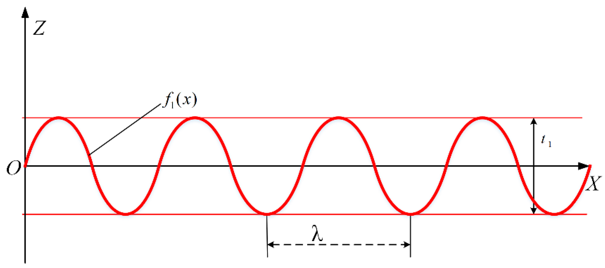
According to the above analysis, the plane microtopography curve of the guide rail in the XOZ plane can be obtained from Equation (1), as detailed in Equation (2). The schematic diagram of its surface microtopography is shown in Figure 5.

$$f_1\left(x\right)={\displaystyle \frac{t_1}{2}}{\displaystyle \sum _{n=1}^{\infty }\frac{1}{n}}\sin \left({\displaystyle \frac{2n\pi }{\lambda }}\cdot x\right),$$

(2)

where $f_1\left(x\right)$ is the microtopography curve of the X-axis guide rail surface in the XOZ plane, and $t_1$ is the linear tolerance of the X-axis guide in the XOZ plane.

Similarly, the microtopography curve of the guide rail surface in the XOY plane is shown in Equation (3), and the schematic diagram of the microtopography of the guide rail surface is shown in Figure 6.

$$f_2\left(x\right)={\displaystyle \frac{t_2}{2}}{\displaystyle \sum _{n=1}^{\infty }\frac{1}{n}}\sin \left({\displaystyle \frac{2n\pi }{\lambda }}\cdot x\right),$$

(3)

where $f_2\left(x\right)$ is the microtopography curve of the X-axis guide rail surface in the XOY plane, and $t_2$ is the linear tolerance of the X-axis guide in the XOY plane.

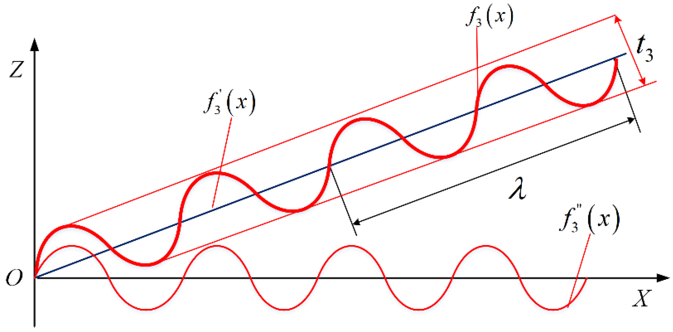
The linear displacement error, pitch angle error, and traverse angle error can be predicted based on the microscopic surface profile curves $f_1\left(x\right)$ and $f_2\left(x\right)$ of the guide rail. The positioning error is primarily influenced by the ball screw’s manufacturing precision, specifically, its cumulative lead error. This cumulative lead error comprises the error profile of the cumulative representative lead, as illustrated in Figure 7.

According to Figure 7, the change in the cumulative lead error can be characterized as a combination of a monotonic function and a Fourier series, as shown in Equation (4):

$$f_3\left(x\right)=f_3^{\prime }\left(x\right)+f_3^{″}\left(x\right)=ax+{\displaystyle \frac{t_3}{2}}{\displaystyle \sum _{n=1}^{\infty }\frac{1}{n}}\sin \left({\displaystyle \frac{2n\pi }{\lambda }}\cdot x\right),$$

(4)

where $f_3\left(x\right)$ is the cumulative lead error for the X-axis guide, $f_3^{\prime }\left(x\right)$ is the cumulative representative lead for the X-axis screw, $f_3^{″}\left(x\right)$ is the X-axis screw’s cumulative representative lead error profile, $t_3$ is the positioning tolerance of the X-axis, and $a$ is an accumulated scaling factor representing the lead.

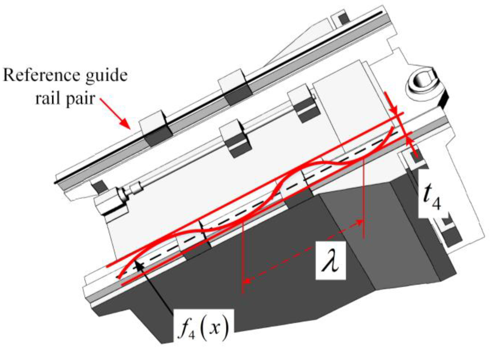
The roll angle error is mainly affected by the parallelism error between guide rail pairs and the slide length. Taking one guide rail as the reference standard, the change in surface microtopography of the other guide rail can be characterized by a Fourier series, as shown in Equation (5). A schematic diagram of the surface and the structure of its microtopography are shown in Figure 8.

$$f_4\left(x\right)={\displaystyle \frac{t_4}{2}}{\displaystyle \sum _{n=1}^{\infty }\frac{1}{n}}\sin \left({\displaystyle \frac{2n\pi }{\lambda }}\cdot x\right),$$

(5)

where $f_4\left(x\right)$ denotes the parallelism error between two guide rail pairs and $t_4$ is the positioning tolerance in the X-axis.

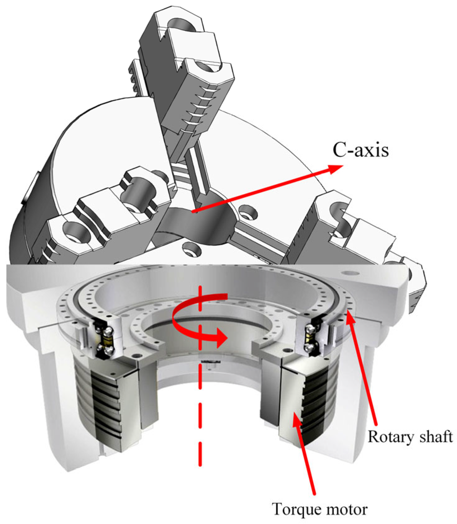
For the C-axis, the rotating shaft is mounted within the upper and lower bores of the spindle box (see Figure 9). The rotation error of the shaft and the surface microtopography of these bores are represented as Fourier series in Equations (6) and (7), respectively. Figure 10 provides a schematic of the surface microtopography.

$$f_1\left(c\right)={\displaystyle \frac{t_{16}}{2}}{\displaystyle \sum _{n=1}^{\infty }\frac{1}{n}}\sin {\theta }_c,$$

(6)

Here, $f_1\left(c\right)$ is the microscopic profile curve of the rotation error of the C-axis, $t_{16}$ is the tolerance of the rotation angle in the C-axis, ${\theta }_c$ is the rotation angle about the C-axis, and $n$ is the order of the Fourier series.

$$f_2\left(c\right)={\displaystyle \frac{t_{17}}{2}}{\displaystyle \sum _{n=1}^{\infty }\frac{1}{n}}\sin {\theta }_c,$$

(7)

Here, $f_2\left(c\right)$ is the surface microtopography curve of the upper and lower bore holes, $t_{17}$ is the radial runout tolerance of the upper and lower bores, ${\theta }_c$ is the rotation angle about the C-axis, and $n$ is the order of the Fourier series.

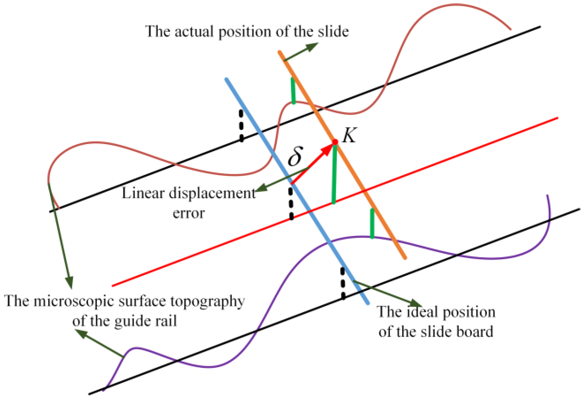
Suppose the carriage moves along the microtopographic curve $f(x)$ of the guide surface, as shown in Figure 11 and Figure 12, using the following notation:

$D$—the width of the carriage;

$L$—the length of the slide;

$K$—the middle point of the slide;

$\epsilon$—angular displacement error;

$\delta$—linear displacement error.

Figure 12 more clearly presents the intrinsic relationship between the microtopography of the rail surface and the geometric errors. The mapping relationships for these two errors can be expressed according to Equations (8)–(12):

$${\delta }_z(x)={\displaystyle \frac{f_1(x_{i-1})+f_1(x_{i+1})}{2}},$$

(8)

$${\epsilon }_y(x)={\displaystyle \frac{f_1(x_{i+1})-f_1(x_{i-1})}{D}},$$

(9)

$${\delta }_y(x)={\displaystyle \frac{f_2(x_{i-1})+f_2(x_{i+1})}{2}},$$

(10)

$${\epsilon }_z(x)={\displaystyle \frac{f_2(x_{i+1})-f_2(x_{i-1})}{D}},$$

(11)

$${\delta }_x(x)=f_3(x),$$

(12)

$f_1(x_i)$ and $f_2(x_i)$ are the function values associated with the curve at a point $x_i$; $f_3(x)$ is the cumulative lead error of the X-axis guide rail; and $D$ is the width of the slide, where $D/\lambda =0.25$.

In addition, the roll angle error is mainly affected by the parallelism error between the two guide pairs and the length of the carriage. According to Figure 8 and Figure 13, the mapping relationship between the microscopic topography and the parallelism and roll angle errors can be obtained using Equation (13):

$${\epsilon }_x(x)={\displaystyle \frac{f_4^{\prime }(x)}{L}}={\displaystyle \frac{f_4(x_{i+1})+f_4(x_{i-1})}{2L}}.$$

(13)

where $f_4(x_i)$ is the function value at a point $x_i$; $f_4^{\prime }(x)$ denotes the parallelism error when the X-axis slide moves at a position $x_i$; and $L$ is the length of the X-axis slide.

With these equations, a mapping model between the X-axis surface microtopography and the relevant geometric errors can be established.

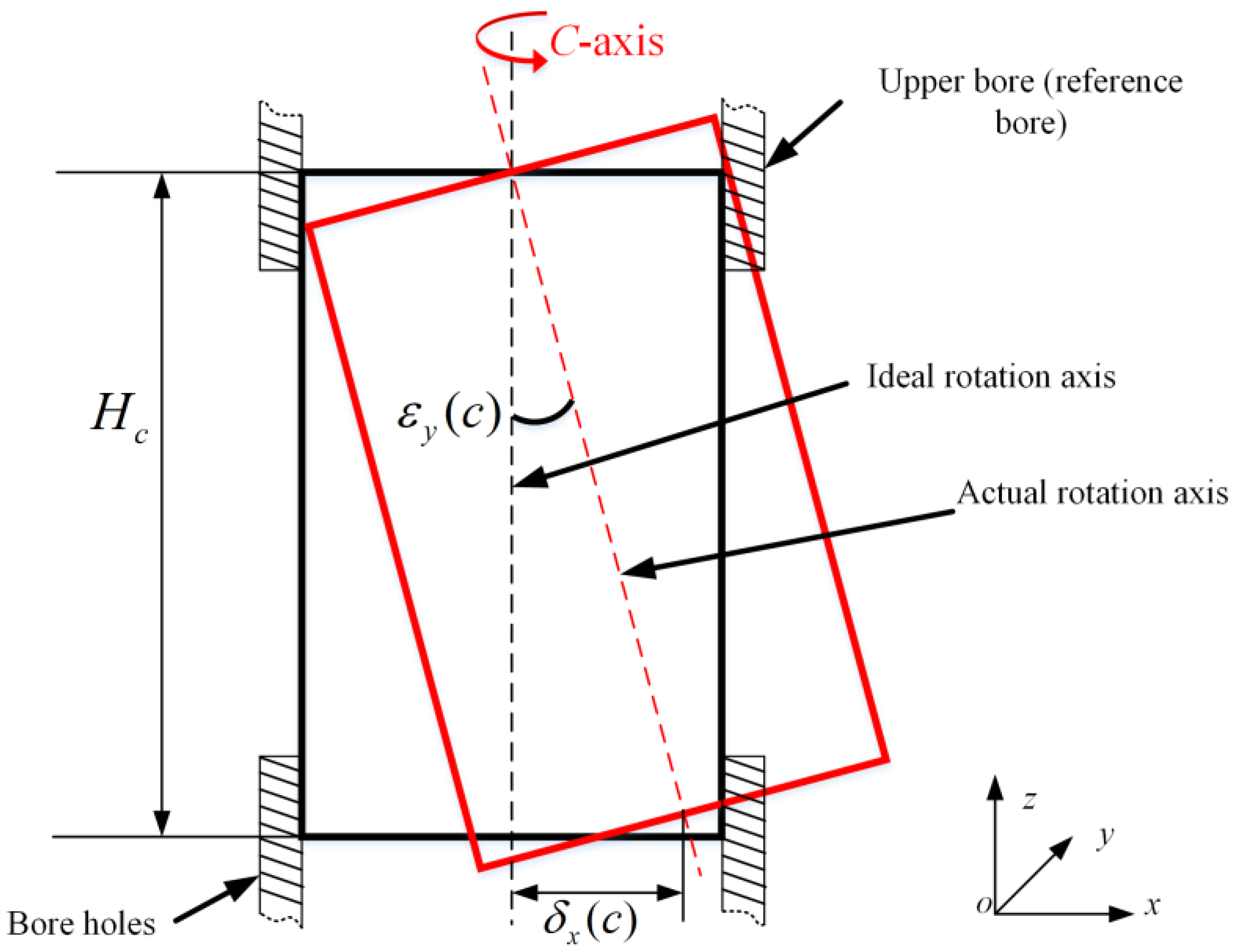
The C-axis is mounted in the upper and lower bores of the spindle housing, according to the relationships between the machine tool’s key components. Figure 14 illustrates the error motion of the C-axis in the XOZ plane. The models describing the mapping relationships between the surface microtopography and geometric errors for the upper and lower bores are presented in Equations (14) and (15), respectively:

$${\delta }_x(c)=f_2(c)\cos {\theta }_c,$$

(14)

$${\epsilon }_y(c)={\displaystyle \frac{{\delta }_x(c)}{H_c}}={\displaystyle \frac{f_2(c)\cos {\theta }_c}{H_c}},$$

(15)

where $f_2(c)$ is the surface microtopography curve of the upper and lower bore holes, and $H_c$ is the length of the C-axis.

Figure 15 shows the error motion of the C-axis in the YOZ plane. The models capturing the relationship between the surface microtopographies of the upper and lower boring holes and the geometric errors ${\delta }_y(c)$, ${\delta }_z(c)$, and ${\epsilon }_x(c)$ are shown in Equations (16) to (18), respectively:

$${\delta }_y(c)=f_2(c)\sin {\theta }_c,$$

(16)

$${\epsilon }_x(c)={\displaystyle \frac{{\delta }_y(c)}{H_c}}={\displaystyle \frac{f_2(c)\sin {\theta }_c}{H_c}},$$

(17)

$${\delta }_z(c)={\displaystyle \frac{t_{18}}{2}}{\displaystyle \sum _{n=1}^{\infty }\frac{1}{n}}\sin {\theta }_c,$$

(18)

where $t_{18}$ is the axial runout tolerance of the C-axis.

The angular positioning error of the C-axis, ${\epsilon }_z(c)$, can be expressed according to the microtopography of the rotational error of the C-axis, as shown in Equation (19):

$${\epsilon }_z(c)=f_1(c),$$

(19)

where $f_1(c)$ is the microscopic profile curve of the rotation error of the C-axis.

Therefore, the rotation error model for the C-axis has been determined.

Geometric errors typically arise after assembly of the machine tools, making it challenging for design engineers to accurately predict these errors during the initial design phase. Reliance on design experience—which is prone to subjective bias—often leads to imprecise predictions. Thus, accurately forecasting geometric errors using tolerance parameters of critical components is crucial in the early stages of machine tool design. The surface microtopography of key CNC machine tool parts serves as a link between tolerance and geometric errors. Consequently, a prediction model for geometric errors that is based on the tolerances of these key components was developed. In particular, first-order Fourier series were employed to predict geometric errors for various axes, which yielded consistent conclusions for other geometric errors.

Based on the above analysis, 25 tolerance parameters corresponding to all 37 geometric errors were determined (as shown in

Table 1. The 25 tolerance parameters corresponding to 37 geometric errors.

Geometric Error	Tolerance Parameter	Geometric Error	Tolerance Parameter	Geometric Error	Tolerance Parameter
${\delta }_x\left(x\right)$	$t_3$	${\delta }_y\left(z\right)$	$t_{10}$	${\delta }_z\left(c\right)$	$t_{18}$
${\delta }_y\left(x\right)$	$t_2$	${\delta }_z\left(z\right)$	$t_{11}$	${\epsilon }_x\left(c\right)$	$t_{17}$
${\delta }_z\left(x\right)$	$t_1$	${\epsilon }_x\left(z\right)$	$t_{10}$	${\epsilon }_y\left(c\right)$	$t_{17}$
${\epsilon }_x\left(x\right)$	$t_4$	${\epsilon }_y\left(z\right)$	$t_9$	${\epsilon }_z\left(c\right)$	$t_{16}$
${\epsilon }_y\left(x\right)$	$t_1$	${\epsilon }_z\left(z\right)$	$t_{12}$	${\epsilon }_{\mathit{xz}}$	$t_{19}$
${\epsilon }_z\left(x\right)$	$t_2$	${\delta }_x\left(b\right)$	$t_{14}$	${\epsilon }_{\mathit{xy}}$	$t_{20}$
${\delta }_x\left(y\right)$	$t_6$	${\delta }_y\left(b\right)$	$t_{15}$	${\epsilon }_{yz}$	$t_{21}$
${\delta }_y\left(y\right)$	$t_7$	${\delta }_z\left(b\right)$	$t_{14}$	${\epsilon }_{\mathit{xb}}$	$t_{22}$
${\delta }_z\left(y\right)$	$t_5$	${\epsilon }_x\left(b\right)$	$t_{14}$	${\epsilon }_{\mathit{bz}}$	$t_{23}$
${\epsilon }_x\left(y\right)$	$t_5$	${\epsilon }_y\left(b\right)$	$t_{13}$	${\epsilon }_{\mathit{xc}}$	$t_{24}$
${\epsilon }_y\left(y\right)$	$t_8$	${\epsilon }_z\left(b\right)$	$t_{14}$	${\epsilon }_{\mathit{yc}}$	$t_{25}$
${\epsilon }_z\left(y\right)$	$t_6$	${\delta }_x\left(c\right)$	$t_{17}$	—	—
${\delta }_x\left(z\right)$	$t_9$	${\delta }_y\left(c\right)$	$t_{17}$	—	—

). The geometric definitions corresponding to these parameters are provided in

Table 2. Geometric definitions of tolerance parameters.

Tolerance Parameter	Definition	Tolerance Parameter	Definition
$t_1$	Linear tolerance of X-axis guide rail in XOZ plane	$t_{14}$	Radial runout tolerance of upper and lower bores of B-axis
$t_2$	Linear tolerance of X-axis guide rail in XOY plane	$t_{15}$	Axial run-out tolerance of B-axis
$t_3$	Positioning tolerance of X-axis screw	$t_{16}$	Tolerance of C-axis rotation angle
$t_4$	Parallelism tolerance between X-axis guide pairs	$t_{17}$	Tolerance of radial circular run-out of upper and lower bores of C-axis
$t_5$	Linear tolerance of Y-axis guide in YOZ plane	$t_{18}$	Axial run-out tolerance of C-axis
$t_6$	Linear tolerance of Y-axis guide rail in XOY plane	$t_{19}$	Squareness tolerance between X- and Z-axes
$t_7$	Positioning tolerance of Y-axis screw	$t_{20}$	Squareness tolerance between X- and Y-axes
$t_8$	Parallelism tolerance between Y-axis guide pairs	$t_{21}$	Squareness tolerance between Y- and Z-axes
$t_9$	Linear tolerance of Z-axis guide rail in XOZ plane	$t_{22}$	Squareness tolerance between X- and B-axes
$t_{10}$	Linear tolerance of Z-axis guide rail in YOZ plane	$t_{23}$	Squareness tolerance between Z- and B-axes
$t_{11}$	Z-axis screw positioning tolerance	$t_{24}$	Squareness tolerance between X- and C-axes
$t_{12}$	Parallelism tolerance between Z-axis guide pairs	$t_{25}$	Squareness tolerance between Y- and C-axes
$t_{13}$	Tolerance of B-axis rotation angle	—	—

.

2.2. Spatial Motion Error Model

Multi-body system modeling was performed following the scheme shown in Figure 16.

The position vector of the point to be machined in the workpiece coordinate system is defined in Equation (20):

$$\begin{array}{l}\left\{P_{we1}\right\}={\displaystyle \prod \left({[Si\_j]}_p{[Si\_j]}_{pe}{[Si\_j]}_s{[Si\_j]}_{se}\right)\cdot \left\{r_{W1}\right\}=}\\ {[S0\_6]}_p{[S0\_6]}_{pe}{[S0\_6]}_s{[S0\_6]}_{se}\cdot \begin{array}{cc}& \end{array}\\ {[S6\_7]}_p{[S6\_7]}_{pe}{[S6\_7]}_s{[S6\_7]}_{se}\cdot \left\{r_{W1}\right\}\end{array}$$

(20)

In this formula, $\left\{p_{we1}\right\}$ is the position matrix of point P in the workpiece coordinate system $O_i-x_i{y}_i{z}_i$;

• $\left\{r_{W1}\right\}$ is the position matrix of point P in the workpiece coordinate system $O_i-x_i{y}_i{z}_i$;
• ${[Si\_j]}_p$ is the J body relative to the I body ideal static homogeneous transformation matrix between the bodies;
• ${[Si\_j]}_{pe}$ is the actual static homogeneous transformation matrix between the J body and the I body;
• ${[Si\_j]}_s$ is the homogeneous transformation matrix for the ideal inter-body motion between the J body and the I body;
• ${[Si\_j]}_{se}$ is the homogeneous transformation matrix for the actual inter-body motion of the J body relative to the I body.

The position vector of the tool center point in the machine tool’s coordinate system is shown in Equation (21):

$$\begin{array}{l}\left\{P_{te1}\right\}={[S0\_1]}_p{[S0\_1]}_{pe}{[S0\_1]}_s{[S0\_1]}_{se}\cdot \\ \begin{array}{ccc}& & \end{array}{[S1\_2]}_p{[S1\_2]}_{pe}{[S1\_2]}_s{[S1\_2]}_{se}\cdot \\ \begin{array}{ccc}& & \end{array}{[S2\_3]}_p{[S2\_3]}_{pe}{[S2\_3]}_s{[S2\_3]}_{se}\cdot \\ \begin{array}{ccc}& & \end{array}{[S3\_4]}_p{[S3\_4]}_{pe}{[S3\_4]}_s{[S3\_4]}_{se}\cdot \\ \begin{array}{ccc}& & \end{array}{[S4\_5]}_p{[S4\_5]}_{pe}{[S4\_5]}_s{[S4\_5]}_{se}\cdot \left\{r_{T1}\right\}\end{array}.$$

(21)

In this formula,

• $\left\{p_{te1}\right\}$ is the position matrix of point P in the tool coordinate system $O_i-x_i{y}_i{z}_i$.
• $\left\{r_{T1}\right\}$ is the position matrix of point P in the tool coordinate system $O_i-x_i{y}_i{z}_i$.

In the actual machining process, in order to achieve precision machining, the point to be machined in the workpiece coordinate system and the center point of the tool must coincide, such that Equation (22) is satisfied:

$$P_{we1}=P_{te1}.$$

(22)

In summary, the position vector of the tool center point in the workpiece coordinate system during the actual machining process can be obtained from Equations (20)–(22), as shown in Equation (23):

$$\begin{array}{l}\left\{r_{W1}\right\}=\left\{{[S0\_6]}_p{[S0\_6]}_{pe}{[S0\_6]}_s{[S0\_6]}_{se}\cdot \right.\\ \begin{array}{ccc}& & \end{array}{\left.{[S6\_7]}_p{[S6\_7]}_{pe}{[S6\_7]}_s{[S6\_7]}_{se}\right\}}^{-1}\cdot \\ \begin{array}{ccc}& & \end{array}{[S0\_1]}_p{[S0\_1]}_{pe}{[S0\_1]}_s{[S0\_1]}_{se}\cdot \\ \begin{array}{ccc}& & \end{array}{[S1\_2]}_p{[S1\_2]}_{pe}{[S1\_2]}_s{[S1\_2]}_{se}\cdot \\ \begin{array}{ccc}& & \end{array}{[S2\_3]}_p{[S2\_3]}_{pe}{[S2\_3]}_s{[S2\_3]}_{se}\cdot \\ \begin{array}{ccc}& & \end{array}{[S3\_4]}_p{[S3\_4]}_{pe}{[S3\_4]}_s{[S3\_4]}_{se}\cdot \\ \begin{array}{ccc}& & \end{array}{[S4\_5]}_p{[S4\_5]}_{pe}{[S4\_5]}_s{[S4\_5]}_{se}\cdot \left\{r_{T1}\right\}\end{array},$$

(23)

$$r_{W1}={\left(\begin{array}{cccc}{r}_{Wx1}& r_{Wy1}& r_{Wz1}& 1\end{array}\right)}^T.$$

(24)

Under the ideal motion condition for the machine tool, each error parameter value is 0. The position vector $r_{W1}^i$ from the tool center point to the workpiece coordinate system under ideal conditions can be obtained from Equation (25):

$$r_{W1}^i={\left(\begin{array}{cccc}{r}_{Wx1}^i& r_{Wy1}^i& r_{Wz1}^i& 1\end{array}\right)}^T.$$

(25)

Subtracting Equation (25) from Equation (24), the spatial motion error model of the machine tool can be obtained, defined in Equation (26):

$$E=r_{W1}-r_{W1}^{\prime }={\left(\begin{array}{cccc}{E}_{x1}& E_{y1}& E_{z1}& 1\end{array}\right)}^T.$$

(26)

2.3. Tolerance Sensitivity Analysis

To identify the tolerance parameters that contribute the most to the peak value of the spatial motion error, a gradient-based sensitivity index is defined as follows:

Three types of geometric errors exist in milling processes: position-dependent linear displacement errors, angular displacement errors, and position-independent squareness errors.

According to the type of tolerance, the expression for calculating the geometric error sensitivity of linear tolerance and angular tolerance is given by Formula (27):

$$\Delta E_i=\left[\begin{array}{c}\Delta E_{ix}\\ \Delta E_{iy}\\ \Delta E_{iz}\end{array}\right]={\displaystyle \frac{\partial E_i}{\partial G_i}}\cdot {\displaystyle \frac{d{G}_i}{d{t}_i}},$$

(27)

where $\Delta E_i$ is the increment in tolerance $t_i$ with respect to the spatial motion error; $E_i$ is the position component of the spatial motion error; $G_i$ denotes the geometric error parameters of component $i$ of the machine tool; and $t_i$ are the tolerance variables associated with the $i$th error parameter.

$$\Delta E_{ti}=\sqrt{{\left(\Delta E_x\right)}^2+{\left(\Delta E_y\right)}^2+{\left(\Delta E_z\right)}^2},$$

(28)

where $\Delta E_{ti}$ denotes the sensitivity of the tolerance $t_i$ to spatial motion errors.

Squareness tolerance:

As the geometric error source parameter of squareness tolerance is independent of the change in position, the default parameter does not change, and the increment coefficient is 1, namely, $\Delta G_i=1$, as shown in Equation (29):

$$\Delta G_j={\displaystyle \frac{d{G}_j}{d{t}_j}}=1.$$

(29)

Therefore, the expression for analyzing the geometric error sensitivity for squareness tolerance is given by Equation (30). The comprehensive spatial error sensitivity is then characterized by Equation (31).

$$\Delta E_i=\left[\begin{array}{c}\Delta E_{ix}\\ \Delta E_{iy}\\ \Delta E_{iz}\end{array}\right]={\displaystyle \frac{\partial E_i}{\partial G_i}},$$

(30)

$$\Delta E_{ti}=\sqrt{{\left(\Delta E_x\right)}^2+{\left(\Delta E_y\right)}^2+{\left(\Delta E_z\right)}^2}.$$

(31)

where $\Delta E_i$ is the increment in tolerance $t_i$ with respect to the spatial motion error; $E_i$ is the spatial motion error position component; $G_i$ denotes the geometric error parameters of component $i$ of the machine tool; and $\Delta E_{ti}$ denotes the sensitivity of the tolerance parameter $t_i$ to spatial motion errors.

2.4. NSGA-II

The NSGA-II is an algorithm that searches for the optimal solution by simulating Darwinian genetic selection and natural elimination in biological evolution. This algorithm is simple, universal, robust, and suitable for parallel processing. It is widely used in various fields, especially in certain classical applications that involve complex and large non-linear and multi-objective mechanical system design optimization. The NSGA-II is superior to other optimization algorithms in a lot of aspects; for instance, due to its lower risk of falling into local optima during the optimization process, optimal solutions are more conveniently obtainable and accurate.

2.4.1. Algorithm Principle and Improvement

The NSGA-II is a multi-objective optimization algorithm based on the principle of biological evolution, which searches for optimal solutions by simulating natural selection and genetic mutation processes. Based on the standard NSGA-II, adaptive crossover and mutation operators are introduced in this study to improve the performance of the algorithm in tolerance optimization.

Standard NSGA-II Core Mechanism

Non-dominant ordering involves categorizing a population into non-dominant strata by assessing dominance among individuals. For minimization problems, solution A dominates solution B if A is no worse than B in all objectives and strictly better than B in at least one objective. The sorting process proceeds as follows:

• Count the number of times each individual is dominated and the set of dominated individuals;
• Individuals with zero dominance constitute the first-level non-dominant front;
• Perform iterative calculation of non-dominant fronts for the remaining individuals until all individuals have been sorted.

The crowding degree is calculated to measure the distribution uniformity of individuals in the population, using Formula (32):

$$C{D}_i={\displaystyle {\sum }_{m=1}^M\frac{f_m(i+1)-f_m(i-1)}{f_m^{\max }-f_m^{\min }}},$$

(32)

where $M$ is the number of objective functions. For the ith individual, $f_m(i)$ represents the value of the mth objective function, and $f_m^{\max }$ and $f_m^{\min }$ are the maximum and minimum values of the mth objective function, respectively.

Regarding the elite retention strategy, parent and offspring populations (of size 2N) are merged, with the top N individuals after non-dominant sorting selected to ensure that good genes are retained.

Improvements Made to the NSGA-II

According to the characteristics of the machine tool tolerance optimization problem, the following improvements are proposed in this study.

The adaptive crossover probability is defined as

$$p_c=0.9+0.1\cdot randn(),$$

(33)

which is dynamically adjusted using a normal distribution. This allows the exploration and development capabilities in the evolution process to be more balanced.

The adaptive variation distribution index is defined as

$${\eta }_m=15+10\cdot rand(),$$

(34)

where the mutation step size is dynamically adjusted according to the population diversity, improving the ability of the algorithm to jump out of local optima. A flowchart indicating the processes in the NSGA-II is shown in Figure 17.

2.4.2. Parameter Configuration and Experimental Determination

Based on an orthogonal experimental design and sensitivity analysis, the optimal parameter configuration for the tolerance optimization problem was obtained. It is shown in

Table 3. NSGA-II parameter configuration.

Parameter	Symbol	Value	Determination Basis
Population size	$N$	150	Balance calculation efficiency and solution diversity determined via 20 repeated experiments
Maximum number of iterations	$G_{\max }$	300	Ensure convergence of algorithm; HV value tends to stabilize after 200 generations
Crossover probability	$p_c$	Adaptive (0.8–1.0)	Dynamic adjustment based on normal distribution; mean is 0.9
Mutation probability	$p_m$	${\displaystyle \raisebox{1ex}{$1$}\!\left/ \!\raisebox{-1ex}{$n_{\mathrm{var}}$}\right.}$	Approximately 0.04 ($n_{\mathrm{var}}$ = 25 tolerance parameters)
Cross-distribution index	${\eta }_c$	28	Compared with the standard value, it enhances the local search ability
Variation distribution index	${\eta }_m$	20	Adaptive adjustment range of 15–25

.

2.4.3. Design Standards and Constraints of Machine Tool Spatial Motion Error

According to the design standard of the machine tool, the constraint conditions for spatial motion error were set as follows:

$$\begin{array}{c}E{x}_{\max }=0.03 \mathrm{mm}.\\ E{y}_{\max }=0.03 \mathrm{mm}.\\ E{z}_{\max }=0.03 \mathrm{mm}.\end{array}$$

(35)

with the tolerance parameter constraints

$$t_i>0, i=1,2,\dots ,25.$$

2.4.4. Multi-Objective Optimization Model Construction

Objective Function Definition

The first objective function (sum of weighted tolerance bandwidths) is

$$\min f_1(t)={\displaystyle {\sum }_{i=1}^{25}\Delta E_{ti}}\cdot t_i,$$

(36)

where $\Delta E_{ti}$ is the sensitivity for the tolerance parameter of item $i$.

The second objective function (maximum machining error) is

$$\min f_2(t)=\max (\left|Ex\right|,\left|Ey\right|,\left|Ez\right|),$$

(37)

where x, y, and z are the directions in which the spatial motion error is maximal.

Therefore, the multi-objective optimization problem is defined as

$$\min F(t)={\left[f_1(t),f_2(t)\right]}^T,$$

(38)

while satisfying the constraints

$$\left\{\begin{array}{l}Ex\le 0.03 \mathrm{mm}\\ Ey\le 0.03 \mathrm{mm}\\ Ez\le 0.03 \mathrm{mm}\\ t_i>0, i=1,2,\dots ,25\end{array}\right..$$

(39)

3. Simulation Results and Discussion

3.1. Geometric Error Measurement Results

Using the measurement method described in Section 2.1.2, the geometric errors of the X-axis were obtained. The discrete data points are depicted as blue scattered points in Figure 18. The red curve in the same figure represents the geometric error prediction model. The coefficient of determination, R², is a metric used to assess the curve’s goodness of fit. To validate the effectiveness of this data-fitting approach, the R² values for each fitted curve were calculated. The results demonstrate that this data-fitting method yields high accuracy, indicating that the fitted curves can reliably substitute the measured values.

3.2. Tolerance Sensitivity Results

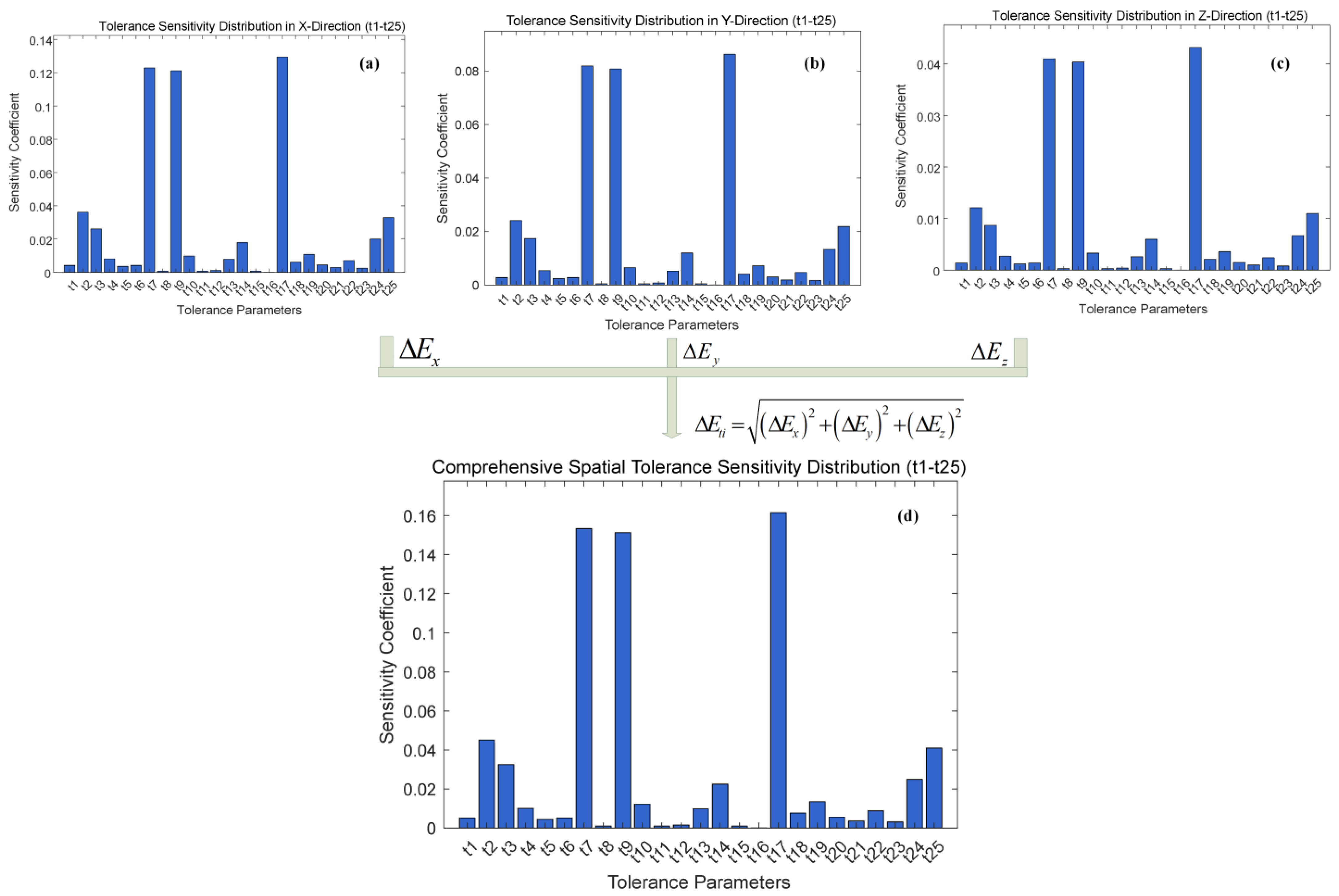
The impact of various tolerance parameters on the volume error of five-axis machine tools varies considerably. Relying solely on design experience to assign weights to these parameters can lead to subjectivity in tolerance allocation. Thus, quantitatively determining the weight coefficient for each tolerance parameter is essential to accurately guide the optimal tolerance allocation for machine tools. The distribution of the sensitivity coefficients $\Delta E_{ti}$ for the 25 tolerance parameters is shown in Figure 19.

3.3. Multi-Objective Optimization Results

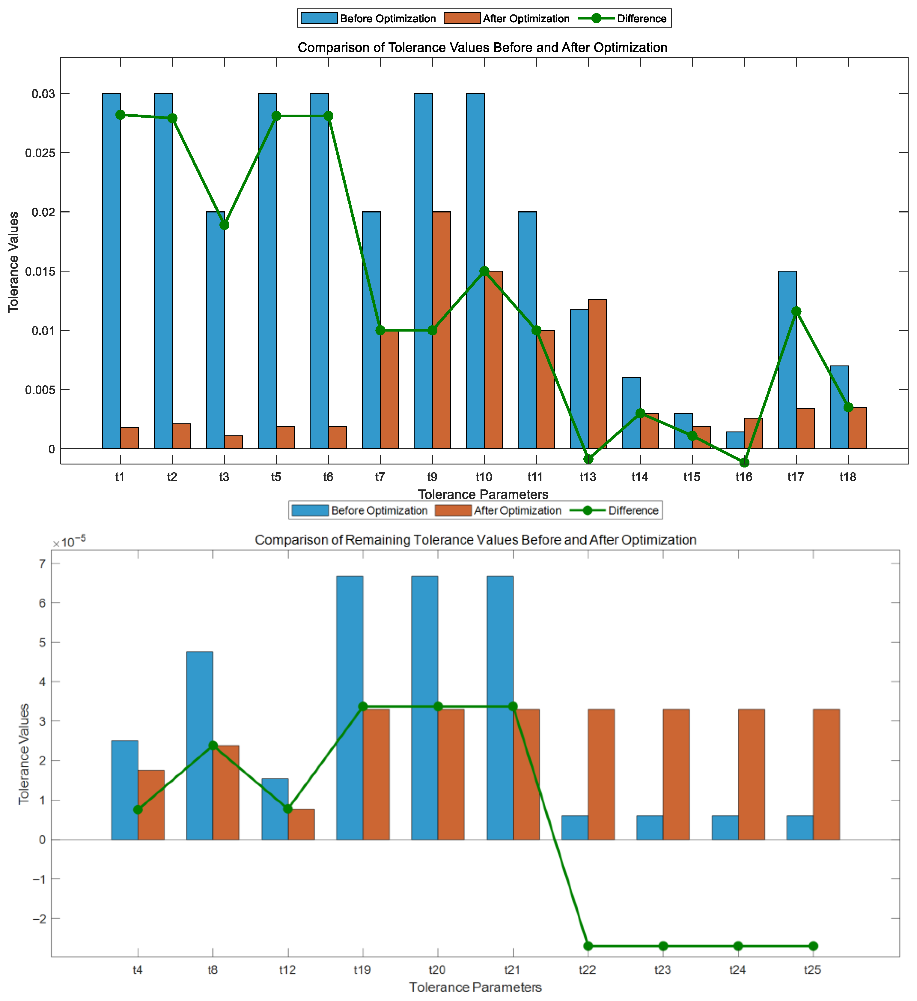
When comparing the tolerance parameter values before and after optimization, a positive difference between the two indicates the tolerance has been relaxed. Conversely, a negative difference means that the tolerance has been tightened. Therefore, the tolerance optimization allocation’s effectiveness can be demonstrated by comparing the tolerance parameter values before and after optimization.

To more intuitively demonstrate the final tolerance optimization allocation scheme’s advantages, the tolerance parameter values before and after optimization are compared using bar charts (Figure 20).

3.4. Optimization Results and Convergence Analysis of NSGA-II

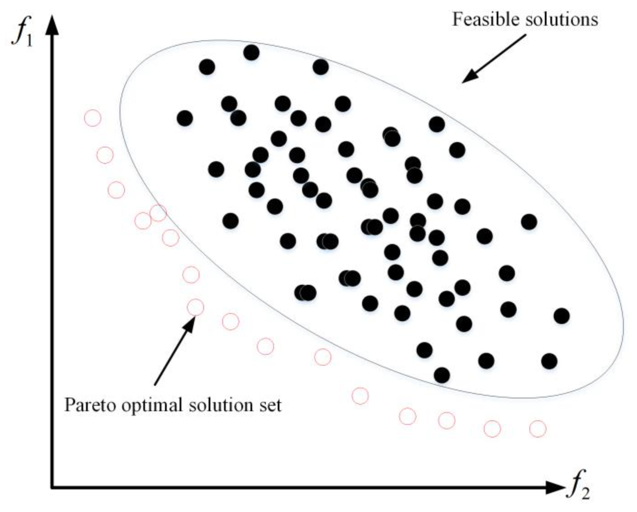
The improved algorithm converged within about 200 generations. The final Pareto solution set (Figure 21) consisted of 27 non-dominated solutions, providing a wide range of options for the design.

4. Conclusions

In the precision optimization of five-axis CNC machine tools, tolerance optimization directly affects the overall machining accuracy. In this study, we designed a multi-objective tolerance optimization method based on sensitivity theory and the NSGA-II algorithm, and achieved the following main results:

(1)

A mapping model of tolerance–surface topography–geometric error was established. The microscopic topography features were characterized using the Fourier series, enabling the prediction of geometric errors in the design stage.

(2)

A tolerance-driven prediction model of the overall machining error was constructed based on the multi-body system theory.

(3)

A gradient-based sensitivity index was innovatively proposed to quantify the influence weight of tolerances on the spatial error. This index effectively identifies the tolerance parameters that have the most significant impact on the peak value of the machining error.

(4)

A multi-objective tolerance optimization model was established. With 25 tolerance bandwidths as variables, under the constraint of spatial error, the NSGA-II algorithm was used to simultaneously optimize the minimization of machining error and the tolerance control cost (the weighted sum of tolerance parameters).

Simulations and applications showed that after optimization, the key tolerances were significantly relaxed, and the manufacturing cost was indirectly reduced, all while ensuring the accuracy meets the standard. The results have been successfully applied to the design of a machine tool.

References

1. Guo, Z.; Zhang, S.; Shi, J.; Sun, J. A modified method for measuring geometric errors of rotary axes based on sensitivity analysis and error simulation. Measurement 2025, 242, 115968. [Google Scholar] [CrossRef]
2. Guevel, F.; Viprey, F.; Euzenat, C.; Fromentin, G.; Masciantonio, U. Geometric error compensation through position feedback modification and comparison of correction strategies in 3-axis machine-tool. J. Manuf. Process. 2025, 150, 213–223. [Google Scholar] [CrossRef]
3. Vázquez, E.; Gomar, J.; Ciurana, J.; Rodríguez, C.A. Evaluation of machine-tool motion accuracy using a CNC machining center in micro-milling processes. Int. J. Adv. Manuf. Technol. 2015, 76, 219–228. [Google Scholar] [CrossRef]
4. Švéda, J.; Chládek, Š.; Hornych, T.; Kozlok, T.; Smolík, J. Increasing Machining Accuracy Based on CNC Machine Tool Correction Data by Using Ad Hoc Modification. Machines 2022, 10, 288. [Google Scholar] [CrossRef]
5. Jedrzejewski, J.; Kwasny, W. Development of machine tools design and operational properties. Int. J. Adv. Manuf. Technol. 2017, 93, 1051–1068. [Google Scholar] [CrossRef]
6. Zimmermann, N.; Müller, E.; Lang, S.; Mayr, J.; Wegener, K. Thermally compensated 5-axis machine tools evaluated with impeller machining tests. CIRP J. Manuf. Sci. Technol. 2023, 46, 19–35. [Google Scholar] [CrossRef]
7. Chen, H.; Tang, Q.; Li, X.; Yang, Y.; Qiao, P. Optimization of five-axis tool grinder structure based on BP neural network and genetic algorithm. Int. J. Adv. Manuf. Technol. 2024, 133, 2565–2582. [Google Scholar] [CrossRef]
8. Song, L.; Sun, T.; Jia, R.; Liu, H.; Zhao, X. An error allocation method for five-axis ultra-precision machine tools. Int. J. Adv. Manuf. Technol. 2024, 130, 2601–2616. [Google Scholar] [CrossRef]
9. Wei, B.; Zhu, S.; Xie, R.; Bi, Q. Identification of geometric errors of five-axis machine tool through volumetric error measurement. J. Phys. Conf. Ser. 2025, 3091, 012001. [Google Scholar] [CrossRef]
10. Nojehdeh, M.V.; Arezoo, B. Functional accuracy investigation of work-holding rotary axes in five-axis CNC machine tools. Int. J. Mach. Tools Manuf. 2016, 111, 17–30. [Google Scholar] [CrossRef]
11. Zhang, S.; He, C.; Liu, X.; Xu, J.; Sun, Y. Kinematic Chain Optimization Design Based on Deformation Sensitivity Analysis of a Five-Axis Machine Tool. Int. J. Precis. Eng. Manuf. 2020, 21, 2375–2389. [Google Scholar] [CrossRef]
12. Wu, H.; Li, X.; Sun, F.; Zhao, Y. A status review of volumetric positioning accuracy prediction theory and static accuracy design method for multi-axis CNC machine tools. Int. J. Adv. Manuf. Technol. 2022, 122, 2139–2159. [Google Scholar] [CrossRef]
13. Fan, J.; Wang, P.; Ren, X. A novel sensitivity analysis of translational axis operation considering key component tolerances. Int. J. Adv. Manuf. Technol. 2022, 118, 1255–1268. [Google Scholar] [CrossRef]
14. Kim, K.; Kim, M.K. Volumetric accuracy analysis based on generalized geometric error model in multi-axis machine tools. Mech. Mach. Theory 1991, 26, 207–219. [Google Scholar] [CrossRef]
15. Ma, W.; Tai, C.; Zhang, L.; He, G.; Xie, Q.; Sun, G.; Qu, L. Multi-stage error compensation with closed-loop quality control in five-axis flank milling of sculptured surface. Int. J. Adv. Manuf. Technol. 2024, 133, 2891–2906. [Google Scholar] [CrossRef]
16. Wu, H.; Zheng, H.; Wang, W.; Xiang, X.; Rong, M. A method for tracing key geometric errors of vertical machining center based on global sensitivity analysis. Int. J. Adv. Manuf. Technol. 2020, 106, 3943–3956. [Google Scholar] [CrossRef]
17. Liu, Y.; Wan, M.; Xiao, Q.-B.; Zhang, W.-H. Identification and compensation of geometric errors of rotary axes in five-axis machine tools through constructing equivalent rotary axis (ERA). Int. J. Mech. Sci. 2019, 152, 211–227. [Google Scholar] [CrossRef]
18. Liu, Y.; Ding, F.; Li, D.; Wu, Y.; Xue, J.; Wang, W.; Qiao, Z.; Wang, B. Machining accuracy improvement for a dual-spindle ultra-precision drum roll lathe based on geometric error analysis and calibration. Precis. Eng. 2020, 66, 401–416. [Google Scholar] [CrossRef]
19. Gao, W.; Ibaraki, S.; Donmez, M.A.; Kono, D.; Mayer, J.R.R.; Chen, Y.-L.; Szipka, K.; Archenti, A.; Linares, J.-M.; Suzuki, N. Machine tool calibration: Measurement, modeling, and compensation of machine tool errors. Int. J. Mach. Tools Manuf. 2023, 187, 104017. [Google Scholar] [CrossRef]
20. Khan, A.W.; Wuyi, C. Systematic Geometric Error Modeling for Workspace Volumetric Calibration of a 5-axis Turbine Blade Grinding Machine. Chin. J. Aeronaut. 2010, 23, 604–615. [Google Scholar] [CrossRef]
21. Fan, J.; Tao, H.; Pan, R.; Chen, D. An approach for accuracy enhancement of five-axis machine tools based on quantitative interval sensitivity analysis. Mech. Mach. Theory 2020, 148, 103806. [Google Scholar] [CrossRef]
22. Guo, J.; Liu, Z.; Li, B.; Hong, J. Optimal tolerance allocation for precision machine tools in consideration of measurement and adjustment processes in assembly. Int. J. Adv. Manuf. Technol. 2015, 80, 1625–1640. [Google Scholar] [CrossRef]
23. Wu, H.; Zheng, H.; Li, X.; Wang, W.; Xiang, X.; Meng, X. A geometric accuracy analysis and tolerance robust design approach for a vertical machining center based on the reliability theory. Measurement 2020, 161, 107809. [Google Scholar] [CrossRef]
24. Liu, H.; Ling, S.; Wang, L.; Yu, Z.; Wang, X. An optimized algorithm and the verification methods for improving the volumetric error modeling accuracy of precision machine tools. Int. J. Adv. Manuf. Technol. 2021, 112, 3001–3015. [Google Scholar] [CrossRef]
25. Li, H.; Li, Y.; Mou, W.; Hao, X.; Li, Z.; Jin, Y. Sculptured surface-oriented machining error synthesis modeling for five-axis machine tool accuracy design optimization. Int. J. Adv. Manuf. Technol. 2017, 89, 3285–3298. [Google Scholar] [CrossRef]
26. Li, X.; Li, C.; Li, P.; Hu, H.; Sui, X. Structural Design and Optimization of the Crossbeam of a Computer Numerical Controlled Milling-Machine Tool Using Sensitivity Theory and NSGA-II Algorithm. Int. J. Precis. Eng. Manuf. 2021, 22, 287–300. [Google Scholar] [CrossRef]
27. Sun, G.; He, G.; Zhang, D.; Sang, Y.; Zhang, X.; Ding, B. Effects of geometrical errors of guideways on the repeatability of positioning of linear axes of machine tools. Int. J. Adv. Manuf. Technol. 2018, 98, 2319–2333. [Google Scholar] [CrossRef]
28. Fan, J.; Wang, P.; Ren, X. A novel global sensitivity analysis method for vital geometric errors of five-axis machine tools. Int. J. Adv. Manuf. Technol. 2021, 117, 3515–3527. [Google Scholar] [CrossRef]
29. Li, Q.; Wang, W.; Jiang, Y.; Li, H.; Zhang, J.; Jiang, Z. A sensitivity method to analyze the volumetric error of five-axis machine tool. Int. J. Adv. Manuf. Technol. 2018, 98, 1791–1805. [Google Scholar] [CrossRef]
30. Jiang, X.; Cui, Z.; Wang, L.; Liu, C.; Li, M.; Liu, J.; Du, Y. Critical geometric errors identification of a five-axis machine tool based on global quantitative sensitivity analysis. Int. J. Adv. Manuf. Technol. 2022, 119, 3717–3727. [Google Scholar] [CrossRef]
31. Tian, W.; Liu, S.; Liu, X. Accuracy design of high precision machine tools using error sensitivity analysis methodology. Proc. Inst. Mech. Eng. Part C J. Mech. Eng. Sci. 2017, 231, 3401–3413. [Google Scholar] [CrossRef]
32. Chen, G.; Ding, S.; Xu, G. Novel method for identifying sensitive geometric errors of CNC machine tools oriented to cylindricity in flank milling. J. Manuf. Process. 2024, 126, 370–381. [Google Scholar] [CrossRef]
33. Fan, J.; Zhang, Y. A novel methodology for predicting and identifying geometric errors of rotary axis in five-axis machine tools. Int. J. Adv. Manuf. Technol. 2020, 108, 705–719. [Google Scholar] [CrossRef]
34. Deb, K.; Pratap, A.; Agarwal, S.; Meyarivan, T. A fast and elitist multi objective genetic algorithm: NSGA-II. IEEE Trans. Evol. Computat. 2002, 6, 182–197. [Google Scholar] [CrossRef]
35. Zhang, Z.; Liu, Z.; Cheng, Q.; Qi, Y.; Cai, L. An approach of comprehensive error modeling and accuracy allocation for the improvement of reliability and optimization of cost of a multi-axis NC machine tool. Int. J. Adv. Manuf. Technol. 2017, 89, 561–579. [Google Scholar] [CrossRef]
36. Demir, G.; Acar Vural, R. Non-Cutting Moving Toolpath Optimization with Elitist Non-Dominated Sorting Genetic Algorithm-II. Appl. Sci. 2024, 14, 4471. [Google Scholar] [CrossRef]
37. Hallmann, M.; Schleich, B.; Wartzack, S. From tolerance allocation to tolerance-cost optimization: A comprehensive literature review. Int. J. Adv. Manuf. Technol. 2020, 107, 4859–4912. [Google Scholar] [CrossRef]
38. ISO 13041-1:2020; Test Conditions for Numerically Controlled Turning Machines and Turning Centres—Part 1: Geometric Tests for Machines with a Horizontal Workholding Spindle. International Organization for Standardization: Geneva, Switzerland, 2020.
Figure 1. Machine tool structure. 0—machine bed; 1—Z-axis; 2—Y-axis; 3—X-axis; 4—B-axis; 5—tool; 6—C-axis; 7—workpiece.
Machines 13 00870 g001
Figure 2. Schematic diagram of the measurement principle of the laser interferometer.
Machines 13 00870 g002
Figure 3. The geometric error measurement setup.
Machines 13 00870 g003
Figure 4. Schematic diagram of the internal structure of the translation axis.
Machines 13 00870 g004
Figure 5. Schematic diagram of the microtopography curve of the X-axis guide rail surface in the XOZ plane.
Machines 13 00870 g005
Figure 6. Schematic diagram of the microtopography curve of the X-axis guide rail surface in the XOY plane.
Machines 13 00870 g006
Figure 7. Schematic diagram of the accumulated error in the pitch of the X-axis guide rail.
Machines 13 00870 g007
Figure 8. Schematic diagram of the parallelism error for the X-axis guide rail.
Machines 13 00870 g008
Figure 9. Schematic diagram of the internal structure of a rotating shaft.
Machines 13 00870 g009
Figure 10. Schematic diagram of the microscopic morphology of the upper and lower bore holes of the C-axis.
Machines 13 00870 g010
Figure 11. Schematic diagram of carriage moving along the microtopographic curve of the guide rail surface.
Machines 13 00870 g011
Figure 12. Angular and linear displacement errors as the slide plate moves along the microtopographic curve of the guide rail surface.
Machines 13 00870 g012
Figure 13. Side view of the parallelism error of the X-axis guide rail surface.
Machines 13 00870 g013
Figure 14. Schematic diagram of the error motion of the C-axis in the XOZ plane.
Machines 13 00870 g014
Figure 15. Schematic diagram of the error motion of the C-axis in the YOZ plane.
Machines 13 00870 g015
Figure 16. Topological structure diagram of a large- and medium-sized five-axis machine tool for multi-body system modeling.
Machines 13 00870 g016
Figure 17. Flowchart of the Non-Dominated Sorting Genetic Algorithm II (NSGA-II). CD, crowding degree.
Machines 13 00870 g017
Figure 18. A comparison between anticipated and actual geometric inaccuracies of the X-axis: (a) Error in X-axis position. (b) Linear displacement error in the Y-direction. (c) Linear displacement error in the Z-direction. (d) Roll error. (e) Yaw error. (f) Pitch error.
Machines 13 00870 g018
Figure 19. Sensitivity coefficient distribution for 25 tolerance parameters in the (a) X-direction, (b) Y-direction, (c) Z-direction, and (d) sensitivity to integrated spatial errors.
Machines 13 00870 g019
Figure 20. Comparisons of the tolerance parameter values before and after optimization.
Machines 13 00870 g020
Figure 21. The Pareto solution set obtained with the NSGA-II.
Machines 13 00870 g021