Article

Voxel-Based Roadway Terrain Risk Modeling and Traversability Assessment in Underground Coal Mines

1
School of Mines, China University of Mining and Technology, Xuzhou 221116, China
2
The State Key Laboratory of Intelligent Mining Equipment Technology, School of Mechanical and Electrical Engineering, China University of Mining and Technology, Xuzhou 221116, China
3
The State Key Laboratory for Fine Exploration and Intelligent Development of Coal Resources, School of Mines, China University of Mining and Technology, Xuzhou 221116, China
*
Author to whom correspondence should be addressed.
Machines 2025, 13(9), 868; https://doi.org/10.3390/machines13090868
Submission received: 29 August 2025 / Revised: 12 September 2025 / Accepted: 15 September 2025 / Published: 18 September 2025
(This article belongs to the Section Machine Design and Theory)

Abstract

Effective roadway environment sensing is critical for intelligent underground vehicle navigation. Dust pollution and complex terrain in underground roadways present key challenges for quantifying passability risks: (1) Over-filtering of dust noise in lidar point clouds can inadvertently remove valuable information. (2) The enclosed and chaotic nature of underground roadways prevents planar information from fully representing spatial constraints. To address these challenges, this paper proposes a method for constructing terrain risk voxels and assessing navigability in coal mine tunnels. First, an improved particle filter combined with image features performs two-stage dust filtering. Second, D-S theory is applied to fuse and evaluate three-dimensional tunnel risks, constructing 3D terrain risk voxels. Finally, navigable spaces are identified and their characteristics quantified to assess passage risks. Experiments show that the proposed dust filtering algorithm achieves 96.7% average accuracy in primary underground areas. The D-S theory effectively constructs roadway terrain risk voxels, enabling reliable quantitative assessment of roadway passability risks.

1. Introduction

Underground coal mines are currently undergoing rapid development in intelligent construction [1,2]. Intelligent auxiliary transport vehicles replacing traditional manually operated vehicles can significantly enhance mine auxiliary transport efficiency, reduce personnel requirements, and ensure transport safety [3,4]. By collecting and modeling the vehicle’s forward travel environment, quantifying and assessing forward passability risks can guide the safe operation of intelligent auxiliary transport vehicles, preventing transport accidents. Compared to surface environments, underground mine tunnels present challenges such as dust interference that degrades sensor data quality. Additionally, tunnels are narrow and elongated with deformable surrounding rock, exhibiting significant variations in cross-sectional profiles at different locations. Furthermore, tunnels often store equipment and materials, creating cluttered environments [5,6]. Consequently, constructing tunnel terrain risk voxels and quantitatively evaluating tunnel passability risks pose substantial challenges.
Lidar is an important means of collecting data [7,8,9,10]; downhole dust seriously affects the quality of lidar point cloud data, with increased data noise and obvious intensity masking. The research around the dust filtering method is mainly divided into two technical paths: one is the classical geometric statistical filtering approach. Ref. [11] proposes a confidence template constructed from lidar reflection intensity combined with neighborhood Euclidean distance for two-stage dust screening. Ref. [12] utilizes Euclidean clustering to eliminate dust outliers first, and then uses normalized weighting ICP to fuse multi-station scans to construct a high-precision roadway model to provide a dust-free benchmark for deformation monitoring. The other path is the deep learning and SLAM fusion approach [13]: ref. [14] combines the pre-processing process of IMU pre-integration and non-ground point segmentation to filter suspended dust before extracting line-plane features, which improves the overall SLAM accuracy and robustness. Xing et al. [13] also proposed a point cloud segmentation method that fuses graph models with deep learning. However, geometric filtering methods are susceptible to limitations imposed by dust distribution within mine tunnels and radar scanning characteristics, leading to under-filtering and misidentification issues. Deep learning-based approaches require substantial point-level annotated data, which is difficult to acquire and incurs high computational overhead. Therefore, dust filtering strategies must be further refined based on the specific characteristics of coal mine dust to enhance the reliability of point cloud environmental perception.
The operating environment for auxiliary transport vehicles underground is complex and dynamic. Current research on vehicle environment risk assessment primarily relies on two-dimensional raster maps [15,16,17,18]. Ref. [19] proposes the “STEP” framework for evaluating and planning autonomous robot navigation in unknown underground environments, using probabilistic models to assess passage risks across map regions. This approach introduces risk-aware cost map learning, employing neural networks to learn the probability distribution of terrain passage cost values and generate passage cost maps reflecting navigational risks. Ref. [20] utilizes the boundaries of unknown forward regions for local navigation and constructs collision risk maps. By calculating edge risk weights within the map, it achieves both rapid and safe autonomous exploration in mining environments. However, ref. [21] based on 2D raster maps struggles to fully account for variations in tunnel contours and three-dimensional spatial information. Therefore, incorporating 3D data and employing more effective information fusion algorithms is necessary to ensure robustness in underground risk assessment.
Based on existing research limitations, constructing terrain risk voxels and assessing passability risks in underground coal mines faces the following challenges: (1) high dust concentrations in mine tunnels lead to false filtering issues, resulting in significant perception errors for point clouds; and (2) 2D raster maps provide limited representation of enclosed, complex underground spaces, failing to fully capture the three-dimensional spatial constraints of mine tunnels.
To address the aforementioned issues, this paper proposes a method for constructing terrain risk voxels and evaluating passability risks in underground mine roadways. Its main contributions are as follows:
  • A dust filtering algorithm based on visual fusion and spatio-temporal geometric particle filtering is proposed. The particle filter was enhanced through spatial neighborhood covariance smoothing and temporal consistency constraints; dust particles were identified via multidimensional state estimation within the particle filter, while visual image features were integrated to suppress false dust detection.
  • A multidimensional D-S fusion algorithm for assessing tunnel terrain and passability risks is proposed. Dempster–Shafer (D-S) evidence theory is an evidence fusion framework for handling uncertain information, based on basic probability assignment and Dempster’s combination rule [22,23]. Tunnel spatial constraints are decomposed into multidimensional risk information, which is then fused using D-S theory to construct a 3D risk voxel model. Based on this terrain risk voxel model and vehicle dimension data, the passable space within the tunnel is extracted. The characteristics of this passable space are analyzed to quantitatively evaluate passability risks.

2. Dust Filtering Algorithm Based on Visual Fusion and Spatio-Temporal Geometric Particle Filtering

2.1. Spatio-Temporal Geometric Particle Filter

2.1.1. Overview of Particle Filters

Particle filtering is a nonlinear filtering technique based on sequential Monte Carlo methods, approximating the posterior probability distribution of the target state through a set of weighted random samples (particles). The fundamental process of standard particle filtering includes the following:
Step 1.
Initialization phase: Generate an initial set of particles x i ( 0 ) , w i ( 0 ) i = 1 N based on the prior distribution.
Step 2.
Prediction phase: Predict the particle state x i ( k | k 1 ) = f x i ( k 1 ) , v i ( k ) according to the system model
Step 3.
Update phase: Using the observed data to update the particle weights w i ( k ) = w i ( k 1 ) · p z ( k ) x i ( k )
Step 4.
Resampling phase: Resampling to avoid particle degradation when the effective particle count is too low
Step 5.
State estimation: The optimal state estimate x ^ ( k ) = i = 1 N w i ( k ) x i ( k ) is obtained by weighted averaging
In the point cloud dust filtering application, each voxel maintains an independent particle filter, and the state vector represents the multidimensional features of the voxel, observed as the voxel feature values of the current frame. In order to make the particle filter more adapted to the dust filtering task, improvements are made in the particle modeling and particle filtering mechanisms as follows.

2.1.2. Particle State Modeling via Fusion of Temporal and Geometric Features

Underground roadway dust spreads randomly in the roadway space over time and has low reflective intensity. Existing point cloud processing methods based on particle filtering usually only consider a single feature of intensity or density, which is difficult to fully reflect the characteristics of underground dust.Therefore, this paper introduces the temporal stability feature and the geometric feature discrimination to jointly characterize the particle state, which is represented by a six-dimensional state vector x = [ I , ρ , S t , I g , P g , S g ] T , where I denotes the intensity, ρ denotes the point density, S t denotes the temporal stability, and P g and S g denote the linearity, flatness and sphericity, respectively. The geometric features are mainly linearity, flatness and sphericity, and for the set of points P = { p 1 , p 2 , , p n } within the voxel, the eigenvalues of the covariance matrix of P are computed λ 1 λ 2 λ 3 , and three structural features are extracted:
Planarity = λ 2 λ 3 λ 1 , Sphericity = λ 3 λ 1 , Linearity = λ 1 λ 2 λ 1
The temporal stability feature is calculated by assessing the temporal consistency of the voxels through the historical observation variance:
S = exp 2.0 × Var I history
In addition, in traditional particle filtering, each particle is usually represented as a deterministic state vector, which lacks effective modeling of state uncertainty and easily leads to particle degradation and degradation of estimation accuracy. Each voxel maintains N particles, and each particle P is represented by a Gaussian distribution, including the state mean μ i R 6 , covariance matrix Σ i R 6 × 6 , and normalized weight W i , which satisfies n = 1 N w n = 1 .

2.1.3. Particle Filtering Mechanism for Spatially Adaptive Neighborhood Covariance Updating

The standard particle filter ignores the spatial correlation between voxels, leading to possible spatial inconsistencies in the state estimation of neighboring voxels, which further reduces the accuracy and stability of the dust filter. In order to effectively solve this problem, this study proposes a spatially adaptive neighborhood covariance updating mechanism that enhances the estimation accuracy and stability in the local region by making full use of the state information of neighboring voxels.
Specifically, the mechanism achieves spatial adaptive covariance smoothing through the following steps:
Step 1.
Determine the spatial neighborhood of the target voxel and obtain the covariance matrix of the voxels in the neighborhood. In order to enhance the spatial continuity and robustness of voxel state estimation, an adaptive neighborhood search strategy is adopted: when the number of neighbors of a voxel is insufficient (|N(v)| < 3), the search radius is dynamically enlarged to ensure that each voxel can effectively fuse sufficient neighborhood information during the state update process, so as to inhibit the influence of local noise on the filtering results and improve the estimation accuracy and spatial consistency.
Step 2.
Calculate the mean of the covariance matrix in the neighborhood as a benchmark for spatial adaptive smoothing
Step 3.
Utilize to update the covariance matrix for the current voxel:
i s m o o t h = α i + ( 1 α ) Σ ¯ n e i g h b o r s
where α is the smoothing factor. Σ is the original covariance matrix of the current voxel, and Σ ¯ n e i g h b o r s is the average of the covariance matrices in the neighborhood.
Step 4.
Further spatial smoothing of particle weights is achieved by the weight adjustment formula:
w i new = ( 1 β ) w i + β w ¯ neighbors
where w ¯ neighbors denotes the average particle weight of neighboring voxels and β is the spatial smoothing strength parameter.

2.2. Voxel Recovery Method for Misfiltered Data Based on Image Feature Fusion

Over-filtering often exists in complex scenes, resulting in the loss of valid voxel information. By fusing visual information and point cloud spatial features, a secondary evaluation of the misfiltered voxels can be realized to effectively recover the misfiltered voxels.

2.2.1. Voxel-Pixel Mapping

Image fusion correction first requires the establishment of an exact projection transformation relationship between 3D voxel coordinates and 2D image coordinates. This process involves transformations between multiple coordinate systems, specifically a rigid body transformation from the world coordinate system to the camera coordinate system, and a perspective projection transformation from the camera coordinate system to the image coordinate system.
Step 1.
Coordinate system transformation. Given the 3D coordinates of a voxel in the world coordinate system P w = [ X w , Y w , Z w , 1 ] T , it is first transformed to the camera coordinate system by means of an external reference matrix as in Equation (5).
P c = T est P w = R t 0 1 X w Y w Z w 1
where R R 3 × 3 is the rotation matrix, t R 3 × 1 is the translation vector, and P c = [ X c , Y c , Z c ] is the 3D coordinates in the camera coordinate system.
Step 2.
Perspective projection transformation. The 3D points under the camera coordinate system are mapped to the normalized image plane by the perspective projection model:
[ x n y n ] = X c Z c Y c Z c
where [ x n y n ] is the normalized image coordinates and Z c is the depth value in the camera coordinate system.
Step 3.
Image coordinate mapping. The corrected normalized coordinates are converted to pixel coordinates by means of the camera internal reference matrix:
u v 1 = K x y z 1 = f 0 c x 0 f c y 0 0 1 x y 1
where K is the camera internal reference matrix, f x ,   f y is the focal length parameter, ( c x , c y ) is the principal point coordinates, and ( u , v ) is the final pixel coordinates.

2.2.2. Image Feature Extraction and Analysis

To assist in determining whether a voxel has been incorrectly filtered, this paper introduces local region features from the image level to describe the neighborhood of voxels projected to the image plane. The image features mainly include three categories: edge features, texture complexit, y and color features.
(1)
Edge characterization. The Sobel gradient operator is utilized to compute the gradient magnitude and directional consistency within the local region, where the gradient magnitude is defined as:
M ( x , y ) = G x ( x , y ) 2 + G y ( x , y ) 2
Gradient direction consistency is quantified by the entropy value of the gradient direction distribution within a localized window, where a lower entropy value represents a more concentrated edge direction and a more significant structural feature in the region.
(2)
Texture characterization. A combination of statistical and structural methods is used to calculate the complexity of local regions of an image, mainly including gray scale standard deviation, which is used to describe the local contrast; Laplace energy, which reflects the complexity of the texture of the local region; the density of the edge points in the region, which is measured by using the Canny operator; and the gray scale entropy, which is used to measure the complexity of the gray scale distribution. The texture complexity feature is obtained by the fusion of these metrics.
(3)
Color features. Color change features reflect the complexity of the color distribution inside the region, which helps to distinguish the background from the object structure from the image, and the color features are obtained by calculating the combination of variance and color entropy of the color channels.
C feature = 0.6 · V a r RGB + 0.4 · E n t r o p y RGB
On the basis of image features, a voxel recovery score evaluation mechanism is constructed by fusing the intensity, geometric structure features, and point density of the point cloud to discriminate whether the filtered voxels are mistakenly deleted or not. The recovery score of voxels is defined as a linear weighted sum of various types of features:
Score = w e · E + w t · T + w c · C + w i · I + w g · G + w d · D
where E: edge feature score; T: texture complexity score; C: color variation score; I: voxel point cloud intensity score; G: geometric structure feature score (evaluated as a combination of linearity, flatness, and sphericity); and D: normalized voxel point density score. w e ,   w t ,   w c ,   w i ,   w g ,   w d is the weighting parameter for each feature.

3. Tunnel Terrain—Access Risk Assessment

3.1. Construction of 3D Risk Voxels for Tunnel Topography Based on D-S Theory

3.1.1. Theoretical Foundations of D-S Theory

D-S theory primarily encompasses the fundamental probability distribution function, the belief function, and the likelihood function. Let Θ = { θ 1 , θ 2 , , θ n } denote the complete set of all possible states, and let its power set 2 Θ encompass all possible combinations of propositions.
The Basic Probability Allocation Function (BPA) is a core element of DS theory. The BPA assigns probability mass to any subset of propositions, expressing the cognitive state of “not knowing.” It satisfies the following conditions:
m : 2 Θ [ 0 , 1 ] , A Θ m ( A ) = 1
Based on BPA, DS theory defines two important metric functions. Belief function (BF) indicates the minimum level of support for a proposition:
B e l ( A ) = B A , B m ( B )
The likelihood function P l : 2 Θ [ 0 , 1 ] represents the maximum possible level of support for the proposition:
P l ( A ) = B A m ( B ) = 1 B e l ( A ¯ )
The belief interval [ B e l ( A ) , P l ( A ) ] constitutes the uncertainty representation of proposition A. The width of the interval reflects the level of cognitive uncertainty. The interval width P l ( A ) B e l ( A ) reflects the degree of cognitive uncertainty, with wider intervals indicating higher levels of uncertainty.
When there are multiple independent sources of evidence, Dempster’s combination rule provides a mathematical framework for evidence fusion. For two BPA functions m 1 and m 2 , the combination result m 1 , 2 is defined as:
m 1 , 2 ( A ) = B C = A m 1 ( B ) · m 2 ( C ) 1 K
where the conflict coefficient K indicates the degree of conflict between the evidence:
K = B C = m 1 ( B ) · m 2 ( C )
When K < 1 , the combination rule is valid; when K 1 , it indicates that there is a serious conflict between the evidence and an improved combination strategy is needed.
DS theory provides a reliable theoretical framework for quantitative fusion of uncertainty information. However, the roadway risk assessment needs to extract effective evidence information from specific roadway spatial features in order to reflect the actual risk condition more accurately. Therefore, this paper improves the evidence source construction, and BPA construction method to obtain accurate and effective risk evidence.

3.1.2. Construction of Three-Dimensional Constrained Evidence Sources

The voxel space is divided into a three-dimensional evaluation grid, and corresponding evidence source information is computed at each evaluation point. As shown in the Figure 1, evidence sources are primarily categorized into width constraint information (blue bands), height constraint information (green bands), and distance constraint information (red bands). For each type of evidence source information, its evidence risk value, evidence reliability, and evidence uncertainty must be further calculated.
It should be noted that the LiDAR coordinate frame (right-handed) is adopted as the primary reference, and camera data are transformed into this frame using the calibrated extrinsic parameters. The axes are defined as follows: the x-axis points forward along the tunnel direction of travel, the y-axis points to the left (width), and the z-axis points upward (height). The horizontal plane is defined as x–y and the vertical cross-section as y–z, with all voxels aligned to this coordinate system.
(1)
Evidence Source Risk Value Calculation
For the width constraint, iterate over all X, Z coordinates, calculate the length of the continuous blank area in the width direction corresponding to each X, Z point, and construct the width constraint risk by the ratio to the total width of the current position; for the height constraint, iterate over all X, Y coordinates, calculate the continuous blank area above each X, Y point, and construct the height constraint risk by the ratio to the total height of the current position; for the distance constraint, iterate over all X, Y, Z coordinates, calculate the continuous blank area in the distance direction of each X, Y, Z point, and construct the distance constraint risk by the ratio with the total distance of the current position.
(2)
Calculation of the reliability of sources of evidence
Reliability of evidence reflects the degree of confidence in the results of the risk assessment. In the lane space, the risk characteristics of neighboring locations should be similar. If the risk assessment of a location is highly consistent with its neighbors, the assessment has high reliability; if there are significant differences, there may be assessment errors or local anomalies.
For each evaluation point p i , search for K nearest neighbor points within a set radius r. Define the 3D risk vector of the current point as R i = [ R i h , R i w , R i d ] T , where R i h ,   R i w ,   R i d denotes the height, width, and distance risk, respectively. For each neighbor point R j N i , compute the Euclidean distance of the risk vector:
d i j = R j R i 2 = ( R j h R i h ) 2 + ( R j w R i w ) 2 + ( R j d R i d ) 2
The spatial consistency measure is defined as the reliability r based on the mean value of the neighborhood risk difference d ¯ i
r i = 1 d ¯ i 3
(3)
Cognitive Uncertainty Calculation of Evidence Sources
Cognitive uncertainty quantifies the degree of assessment uncertainty resulting from conflicting evidence. The three dimensions of alleyway risk values produce inconsistent risk judgments due to differences in the direction of observation, and this conflict directly reflects the uncertainty at the cognitive level.
For each assessment point, the standard deviation of the three risk values for height, width, and distance is calculated, which directly reflects the degree of disagreement in the evidence for the different dimensions, and the degree of inter-dimensional conflict was calculated as:
σ i = 1 3 k { h , w , d } R i k R ¯ i 2
where R ¯ i = 1 3 R i h + R i w + R i d is the average value at risk.
Considering that all three risk values are in the interval [ 0 , 1 ] , the theoretical maximum standard deviation is σ max = 0.577 . when the risk values are 0 ,   0.5 ,   1 . Therefore, the actual standard deviation is normalized:
σ ^ i = σ i σ max
The normalized conflict degree is mapped to the preset uncertainty interval, and the final cognitive uncertainty is calculated as:
U i = U min + σ ^ i · ( U max U min )
where U min ,   U max are the upper and lower bounds of the uncertainty interval, respectively. The lower bound ensures that minimum uncertainty is retained even in the case of perfect agreement, reflecting a cautious approach to absolute certainty; the upper bound limits the maximum level of uncertainty, preventing overly conservative decisions.

3.1.3. BPA Construction Method for Confidence Attenuation

Traditional BPA construction methods are usually based on simple linear mapping or expert knowledge, which is difficult to fully utilize the intrinsic quality information of evidence. In this paper, we propose a BPA construction method based on confidence decay, which can dynamically adjust the probability allocation strategy according to the reliability and uncertainty of the evidence.
A confidence decay model is used to construct the basic probability distribution function. For risk value r, reliability ρ , and uncertainty u, the decay parameters are defined:
σ = σ base + σ adapt ( 1 ρ )
The weighted reliability ρ w = s i g m o i d ( ρ ) , and confidence functions, respectively:
β safe = 1 1 + ( d safe / σ ) 2 , β dangerous = exp d dangerous 2 2 σ 2
The BPA construction process also considers the distributional characteristics of the value at risk. The final probability distribution is:
m ( SAFE ) = ρ w β safe ( 1 r ) ρ w ( β safe ( 1 r ) + β dangerous r )
m ( DANGEROUS ) = ρ w β dangerous r ρ w ( β safe ( 1 r ) + β dangerous r )
m ( UNKNOWN ) = 1 ρ w ( β safe ( 1 r ) + β dangerous r ) .
In the above process, the decay parameters are set with σ base = 0.35 and the adaptive adjustment σ adapt = 0.15 , with σ ranging between [0.35, 0.50] depending on reliability. The confidence attenuation function β safe employs a Cauchy distribution for gradual decay, while β dangerous adopts a Gaussian distribution for sharper decay, so that dangerous masses decay faster than safe ones.

3.1.4. 3D Risk Voxel Raster Construction for Tunnel Topography

The generation of 3D risk voxel rasters is a key step in extending the DS theory fusion results from discrete grid points to a complete 3D space. The process assigns a corresponding risk value to each voxel in the lane space through spatial interpolation and risk propagation mechanisms to form a continuous 3D risk distribution.
Step 1.
Spatial meshing. A 3D evaluation grid covering the entire lane space is first established. Based on the boundary range of the voxel data, generate a regular 3D grid point set G = ( x i , y j , z k ) | x i [ x min , x max ] ,   y j [ y min , y max ] ,   z k [ z min , z max ] .
Step 2.
Multi-source evidence allocation mechanism. For each grid point P i = ( x i , y j , z k ) , organized along X layers, a two-stage matching strategy is used to obtain risk information.
The purpose of the first stage is to determine the X-layer index corresponding to the grid points. The height and width evidence X indexing methods correspond to Equation X. The distance evidence X layer indexing methods correspond to the following equations:
x layer = arg min | x l x i | s . t . x l X layers
x start = max { x l x l x i , x l X layers }
The purpose of the second stage is to find the corresponding risk values within the identified X layers. Height evidence, width evidence, and distance evidence are indexed in the following manner, respectively:
E h ( p i ) = H strips [ x layer ] arg min | y j y i |
E w ( p i ) = W strips [ x layer ] arg min | z k z i |
E d ( p i ) = D strips [ x layer ] arg min | ( y j , z i ) ( y j , z i ) |
where X layers are the preset X-coordinate sampling layers, and H strips , W strips , D strips are the height, width, and distance evidence data structures organized by X layers, respectively. This two-stage strategy ensures spatial localization and improves computational efficiency.
Step 3.
DS theory multi-source fusion. The Dempster combination rule is used to fuse the evidence information in two steps, first fusing the height constraint information with the width constraint information, and then fusing with the distance constraint information to obtain the result:
m h w ( A ) = 1 1 K h w B C = A m h ( B ) · m w ( C )
m final ( A ) = 1 1 K h w d D E = A m h w ( D ) · m d ( E )
where the conflict factor is calculated to take into account inconsistencies between sources of evidence: K = B C = m 1 ( B ) · m 2 ( C ) .
The extreme conflict handling mechanism is enabled when K 0.95 , assigning all masses to the UNKNOWN set.
Step 4.
Risk estimation based on Dempster–Shafer theory. Based on the fusion result of Step 3, a three-focal-set basic probability assignment (BPA) is obtained: m final ( DANGEROUS ) ,   m final ( SAFE ) ,   m final ( UNKNOWN ) . Following Dempster–Shafer theory, the danger is characterized by the belief interval Bel ( DANGEROUS ) , Pl ( DANGEROUS ) , where Bel ( DANGEROUS ) = m final ( DANGEROUS ) , Pl ( DANGEROUS ) = m final ( DANGEROUS ) + m final ( UNKNOWN ) . We adopt the midpoint of this interval as the single-valued risk estimate, which avoids undue conservatism or optimism while explicitly accounting for epistemic uncertainty.

3.2. Risk Assessment of Vehicle Accessibility

The 3D risk voxel raster can visually characterize the risk of the roadway terrain. In this section, the results of the roadway terrain risk assessment are transformed to quantitatively assess the passable risk by extracting the 3D safe-passage space, and then projecting the safe-passage spatial information onto the surface of the terrain in conjunction with the spatial density and height regularity features.

3.2.1. Three-Dimensional Passable Space Recognition Extraction

First, risk voxels are prefiltered using the terrain-risk threshold R thresh , and only the retained voxels are kept for subsequent processing. On the resulting occupancy grid G, let O = { ( p , q , r ) } denote the set of occupied voxels and P ( i , j , k ) denote a free voxel. The Euclidean distance-transform field from each free voxel to the occupied set is then computed as Equation (33)
D ( i , j , k ) = δ · min ( p , q , r ) O ( i p ) 2 + ( j q ) 2 + ( k r ) 2
where δ is the grid resolution. We define the safe-distance threshold d safe as the vehicle’s minimum geometric dimension and label voxels satisfying D ( i , j , k ) > d safe as safe meshes.
Next, invalid safe voxels outside the roadway boundary are removed according to the boundary of the terrain-risk voxel map. Within the remaining safe voxels, traversable space is extracted by connected-component analysis using 26-neighborhood connectivity; connected regions with volumes below a preset minimum are discarded. The largest connected component is taken as the 3D traversable space.
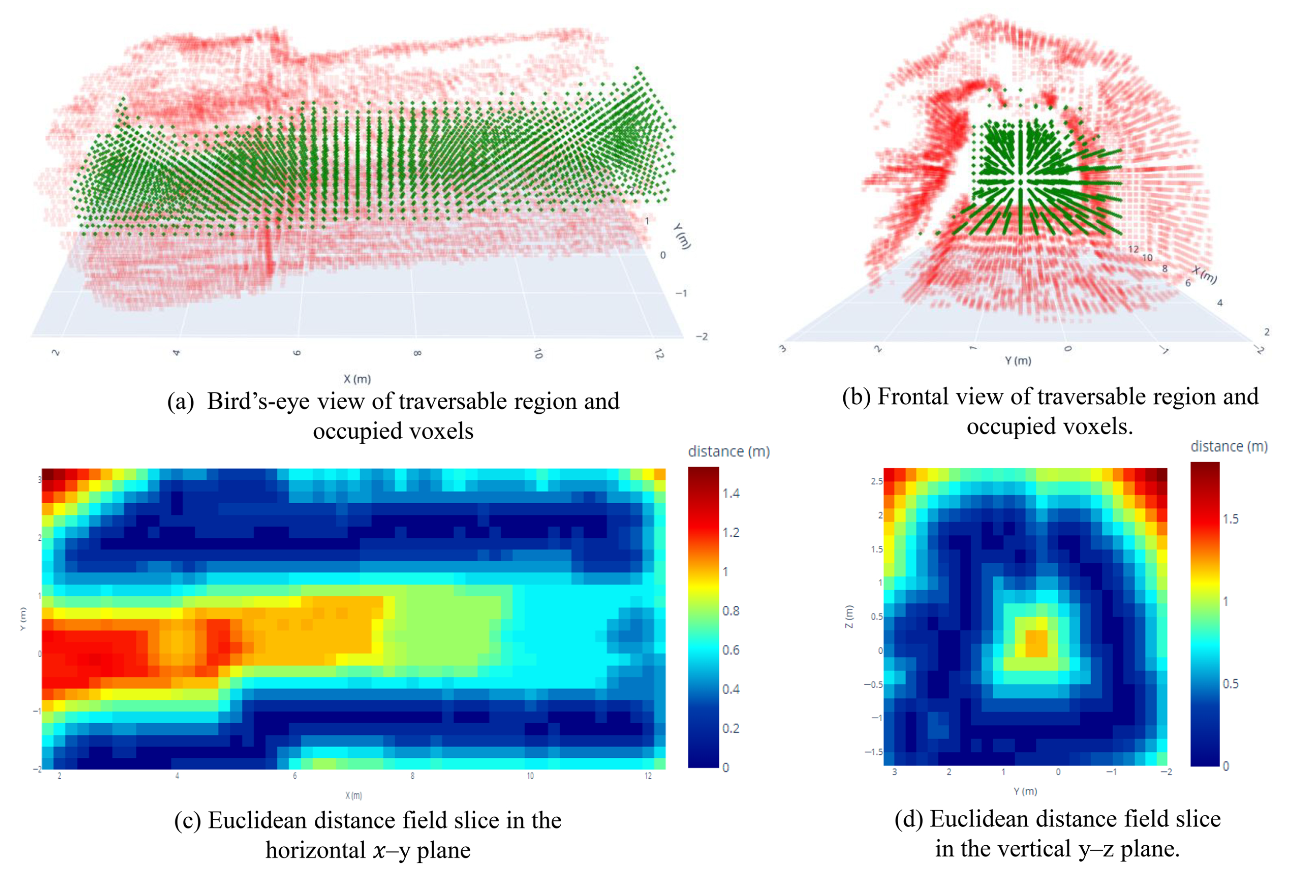
Figure 2 shows the results based on the distance field and safe-voxel threshold. Specifically, (a) and (b) present 3D visualizations of traversable voxels and occupied (risk) voxels from a bird’s-eye and a frontal view, respectively, where green voxels denote safe space and red voxels denote obstacles/risks. (c) and (d) provide examples of Euclidean distance field slices, with (c) showing the horizontal x–y plane and (d) the vertical y–z plane.

3.2.2. Risk Assessment of Accessible Areas

In order to assess the access risk of the 3D passable space, the 3D passable space information was projected onto the terrain surface to quantitatively assess the risk of the passable area.
First, the 3D safe space is projected onto the X-Y plane to generate a 2D convex packet boundary, and the projection points outside the boundary are filtered out. Then, we traverse the projection points, construct a cylindrical region centered on the projection points in the height direction, and extract all the passable space points within the region.
For each cylindrical region, the spatial density attribute ρ i and the height flatness attribute η i are calculated based on the number of passable points and the distribution characteristics of the region. The spatial density attribute ρ i is expressed by the number of passable points in the region, reflecting the passable margin of the region. The height flatness attribute η i reflects the deformation degree of the surrounding rock above the region and is assessed based on the uniformity of the height distribution of the safety points in the region. The distribution uniformity of the height histogram is quantified by the entropy H.
H = k = 1 n p k log p k
Regularity is defined as η i = 1 1 + H . Smaller entropy values indicate that the height distribution is more regular and the risk of accessibility is lower.
By combining the scores of the two attributes, the quantitative results of the passable risk can be obtained.

4. Experiments and Disscusscion

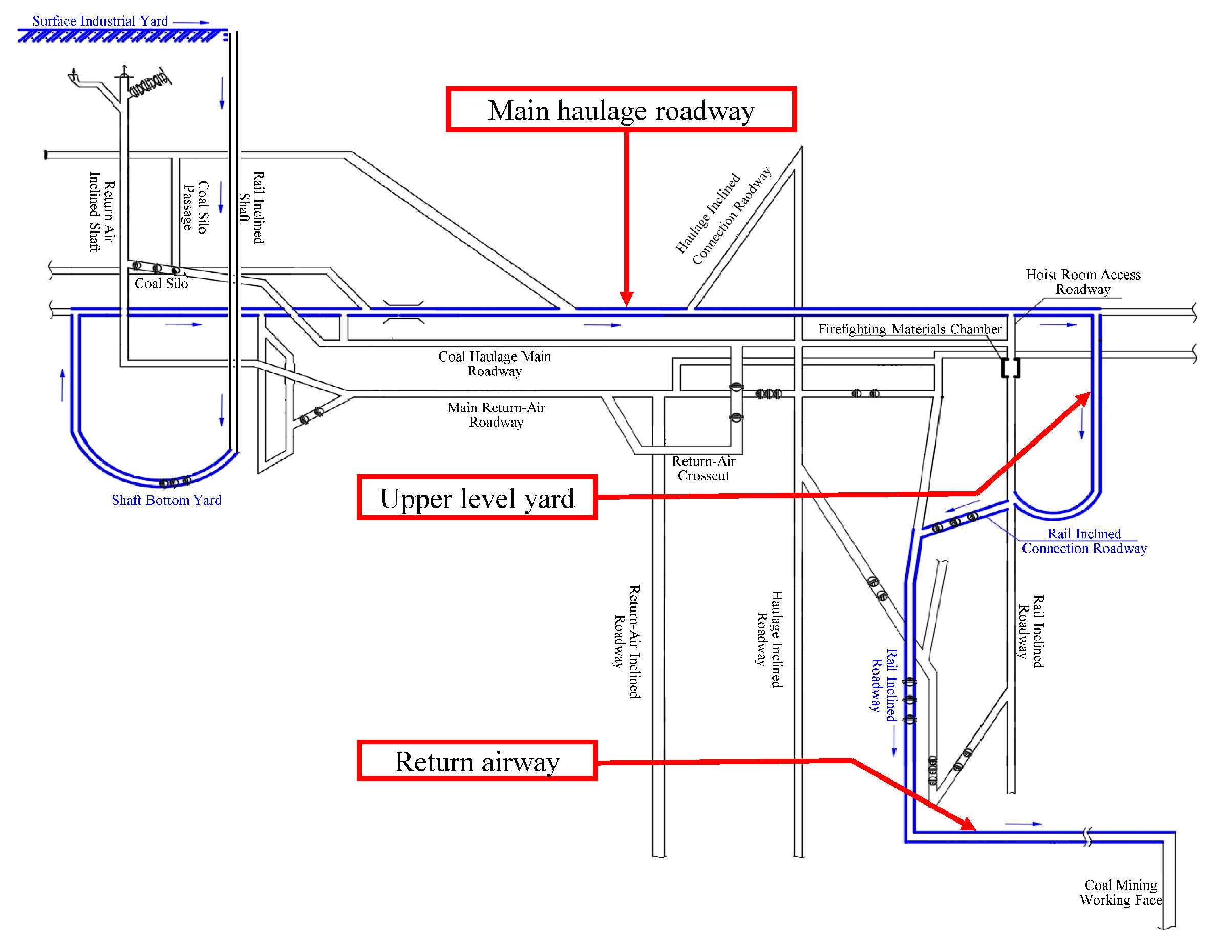
To fully evaluate the method proposed in this paper, LiDAR point cloud data and synchronized image data were collected in the primary travel areas of auxiliary transport vehicles within an underground mine in southwest China. Figure 3 displays the roadway layout of a mining area in this mine, with blue lines marking the travel routes of auxiliary transport vehicles and red boxes delineating the data collection zones: the haulage roadway, upper vehicle yard, and return airway. Experiments were conducted using scene data from six locations within these three zones.
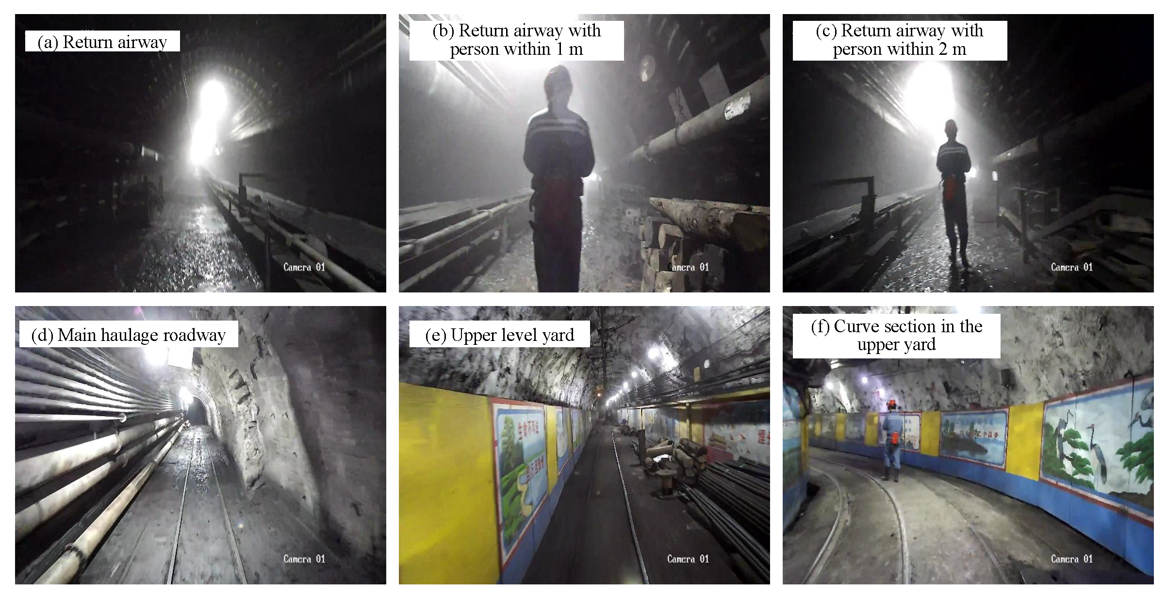
The specific experimental scenarios are illustrated in Figure 4. Figure 4a–c depict the return airway scenario, Figure 4d shows the rail transport main roadway, while Figure 4e,f represent the straight and curved sections of the upper vehicle yard respectively. The return airway presents a complex environment with high dust concentration and poor lighting conditions. The rail transport main roadway and upper yard constitute the primary operational scenarios for auxiliary transport vehicles, featuring clear environmental structures and relatively favorable lighting. Furthermore, to assess the algorithm’s obstacle discrimination capability in complex scenarios and ensure it does not filter out valid obstacle points, factors involving both near-distance and far-distance pedestrians were introduced within the return airway scenario.

4.1. Performance Evaluation of Dust Filtering Algorithms

First, performance testing was conducted on the proposed visual fusion spatio-temporal particle filter algorithm. This algorithm comprises two stages: Stage 1 employs a particle filter for preliminary filtering of point cloud data; Stage 2 integrates visual information to refine the results from Stage 1. Experiments quantified changes in voxel counts across stages, including misfiltered voxels after preliminary filtering and voxels recovered through visual refinement.
To ensure objective and accurate evaluation, misfiltered points were verified manually. Statistics were calculated using voxels within a 5 m forward range, with a voxel resolution of 0.1 m. The maximum number of voxels per frame was capped at 20,000, each configured with 200 particles, and the spatial smoothing radius was set to 0.5 m. Each experimental scenario underwent continuous filtering of five consecutive frames, with the filtered results recorded for each frame.

4.1.1. Overall Analysis

The overall performance of the algorithm is shown in Table 1. By averaging the filtering results across all frames in each scene, the average filtering accuracy of the Stage 1 algorithm was found to be 87.88%, with approximately 12.3% of original voxels removed, accompanied by a certain degree of over-filtering. After correction through visual feature fusion in Stage 2, the average accuracy improved to 96.7%, demonstrating a significant performance enhancement (an increase of 8.82%). The results demonstrate that visual features play a crucial role in restoring structurally deficient regions. The proposed visual fusion strategy effectively mitigates the issue of over-filtering in the initial filtering stage, significantly enhancing the algorithm’s accuracy and stability.
Algorithm performance varies across different scenarios. In the return airway, where dust density is high, the average accuracy across the three scenarios reached 80.96% in Phase 1, with filtering accuracy significantly improving to 95.08% in Phase 2. In the haulage roadway and upper yard, where dust levels are lower, filtering accuracy consistently exceeded 90% in Phase 1. Benefiting from favorable lighting conditions, integrating image features further enhanced Phase 1 accuracy, achieving a maximum filtering accuracy of 98.92% across all three scenarios.

4.1.2. Scenario Analysis

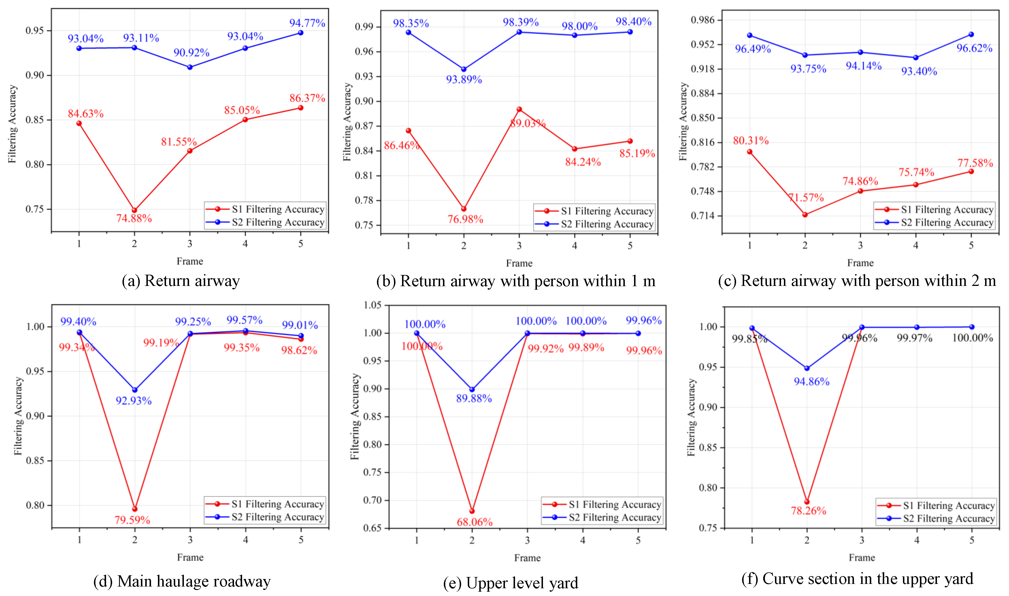
To thoroughly evaluate the algorithm’s dynamic responsiveness and stability, a detailed analysis was conducted on the dust filtering accuracy across different stages using five consecutive frames of data from each scenario. Figure 5 presents a line chart illustrating the temporal performance of the filtering algorithms across various scenarios. It is evident that the second frame in each scenario exhibits a significant decrease in the number of filtered points, primarily attributed to the multi-stage adaptive mechanism designed into the algorithm. The first frame employs relatively lenient single-feature judgment to rapidly establish an initial voxel map. Starting from the second frame, a strict multi-feature comprehensive judgment mechanism is activated, concurrently introducing ICP registration and particle filter updates, significantly elevating the judgment criteria. Additionally, since temporal stability features are not yet fully established in the second frame, the spatial neighborhood smoothing effect is limited, leading to stricter filtering. Starting from the third frame, as historical observation data accumulates and spatial relationships stabilize, filtering accuracy gradually improves and stabilizes, demonstrating the algorithm’s adaptive learning characteristics.
Figure 5a–c illustrate variations in dust filtration accuracy within the return air duct scenario. As personnel appear in the scene, the first-stage filtering at frames 1, 3, 4, and 5 demonstrates superior performance compared with the scenarios in Figure 5a,c when individuals are nearby. This is primarily because the LiDAR does not scan the ground when people are close. Since the rough ground surface of the return air tunnel is the main source of noise points, the first-stage filtering achieves optimal results in the scene depicted in Figure 5b. In the scenario depicted in Figure 5c, as the distance to the person increases and the ground becomes visible, both Stage 1 and Stage 2 filtering performance deteriorates compared to scenarios with people at close range or without people. Compared to the scenario with people at close range, this scenario is darker, and the presence of people increases scene complexity, resulting in weaker filtering performance than the other two scenarios.
Figure 5d–f illustrate dust filtering accuracy variations in the return airway and upper yard scenarios. Both scenarios feature low dust levels and favorable illumination conditions. Except for a sudden drop in filtering accuracy in the second frame due to algorithmic characteristics, the filtering accuracy of both Stage 1 and Stage 2 algorithms exceeded 99% in all other data frames. This demonstrates that the filtering algorithm does not aggressively discard valid data.
The experimental results validate the effectiveness of the two-stage fusion method: the first-stage particle filter provides preliminary filtering, while the second stage compensates for the limitations of particle filtering through image feature fusion. This complementary mechanism ensures robust dust filtering performance across various mine environments.

4.2. Risk Assessment Algorithm Performance Test

The performance evaluation of the proposed risk assessment algorithm is conducted in two stages. (1) Terrain risk assessment: different evidence fusion methods are compared to analyze their effectiveness in evaluating terrain risks. (2) Passability risk assessment: the accuracy of the proposed method in evaluating tunnel passability risks is qualitatively analyzed. Table 2 summarizes the experimental parameter settings, hardware configuration, and runtime performance, where voxel management is optimized using a KD-tree.

4.2.1. Terrain Risk Assessment Performance Analysis

In order to verify the evaluation performance of the proposed D-S evidence theory fusion method in different scenarios, this paper selects the arithmetic average method, the conservative maximum method, the Bayesian inference method, and the entropy weight method as the control methods to compare and evaluate the multidimensional risk fusion effect. In order to quantitatively evaluate the performance of various fusion methods, this paper designs two indicators: risk distribution continuity and risk differentiation. Among them, risk distribution continuity integrates local risk consistency and global spatial autocorrelation, and is used to characterize the continuity and smoothness of the risk field in three-dimensional space; the larger the value, the smoother the risk distribution. Risk differentiation is based on the standard deviation of uniform distribution as a reference, and the symmetric regularity of the risk distribution is used to measure the effectiveness of the method in differentiating between high- and low-risk areas; the larger the value, the stronger the differentiation ability.
Table 3 demonstrates the assessment results of the different methods in the six scenarios. Overall, the D-S evidence theory maintains the optimal score in risk differentiation, and in risk distribution continuity, its performance fluctuates in different scenarios, but overall shows good robustness. In the return airway, the roadway environment is affected by dust, and the three dimensions of the roadway risk vary greatly: when people appear in the return airway, the distance dimension risk fluctuates; when people are in the vicinity (<1 m), the maximum value retention method performs the best in risk distribution continuity; and when people move forward (<2 m), the maximum value retention method risk distribution continuity score decreases by 0.63. The Bayesian inference method, by virtue of its a priori modeling advantage, increases its score from 0.735 to 0.884 and becomes the optimal method. At this time, the DS method risk distribution continuity score is stabilized in the second of the four methods, and the risk differentiation score is always optimal, reflecting that the DS method has a stronger ability to respond to dynamic changes in risk and information fusion. In the transportation alley, the roadway is more structural, the risk changes are fewer, and the D-S method achieves a risk continuity distribution effect similar to that of the best-performing Bayesian method. On the other hand, at the upper yard and its bends where the materials are accumulated, the risk randomness increases with the change of terrain. At this time, the D-S method achieves the optimal risk distribution continuity score, which indicates that it can better integrate the multidimensional risk and more accurately reflect the real risk distribution characteristics in complex environments.
Table 4 further shows the mean (Mean) and standard deviation (Std) of each method for all scenarios. The results show that the DS method obtains the optimal mean and small standard deviation for both risk distribution continuity (0.862 ± 0.026) and risk differentiation (0.915 ± 0.001) metrics, indicating that the method possesses excellent performance and scenario generalization ability. In contrast, the other methods have some limitations. The simple average method ignores the correlation differences among the three risk dimensions. The conservative maximum method has a risk discrimination of 0.898, and the conservative fusion strategy sacrifices the risk discrimination accuracy. The Bayesian method relies heavily on the a priori probability setting, and the standard deviation of risk distribution continuity reaches 0.064, which is insufficient for generalization when the scene changes. The entropy weight method lacks explicit modeling of cognitive uncertainty despite optimizing the weight allocation through information entropy, and its risk distribution continuity score is 0.847 ± 0.03, with a risk discrimination score of 0.896 ± 0.008, which is at odds with the DS method.
The results show that D-S evidence theory, through its intrinsic mechanism of dealing with uncertainty and evidence conflict, can robustly fuse the risks of different dimensions of the roadway, obtain the optimal risk distribution continuity and risk differentiation, and effectively assess the risk of underground roadway terrain.

4.2.2. Accessible Risk Assessment Analysis

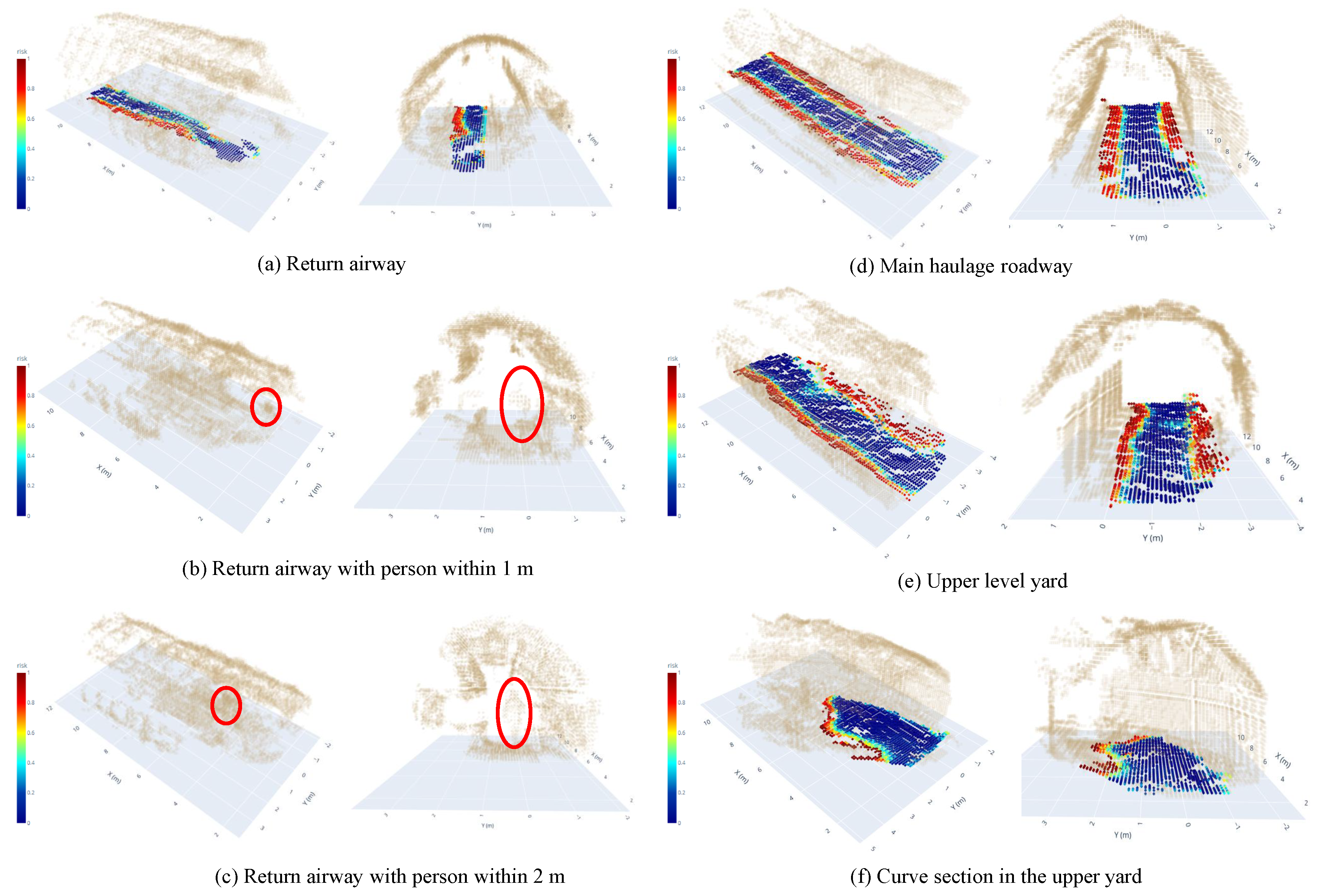
In this study, the effectiveness of the proposed roadway passability risk assessment algorithm is validated under six typical mine roadway scenarios using typical locomotive dimensions (2.96 × 1.12 × 1.80 m, L × W × H). Figure 6 shows the 3D passability risk distribution visualization results in different roadway environments from the front view perspective and the global perspective.
In the return airway, the algorithm successfully identifies the narrow passable area sandwiched between the scraper conveyor and the pipeline (Figure 6a). Since the height change is more drastic on the left side of the roadway, the regularity attribute evaluated by the algorithm enhances the passability risk on the left side, and the height of the area above the scraper on the right side of the passable area is more lenient, so the identified passable area presents a high–low–medium passable risk from left to right. When there is a personnel obstacle in the return alley, the algorithm cannot find the passable connecting area, i.e., it is impassable, because the two scenes have a closer human distance, which is 1 m and 2 m away from the sensor’s effective sensing data (Figure 6b,c), which is smaller than the length dimension of the motor car’s dimensions. In the transportation alley, the algorithm successfully identifies a continuous and regular passable area. In this scenario, there is a narrowing of the width of the alleyway; the algorithm also adaptively recognizes this change; the passable risk as a whole shows obvious spatial regularity, the center area of the alleyway shows a lower risk value, and the risk value of the edge area close to the wall surface of the alleyway is gradually increasing. This gradient distribution verifies the rationality of the algorithm.
In the upper yard, due to the influence of material accumulation in the roadway, the right side of the roadway forms a non-regular passable obstacle. Figure 6e shows that in this case, the non-regular passable obstacle on the right side of the roadway can still be recognized as a high-risk peer area. When the scene changes to the upper yard curve, the risk distribution presents asymmetric characteristics and the risk value of the inner curve side is significantly higher than the outer curve side, which is highly consistent with the actual safety needs of the vehicle turning.
The experimental results show that through the two-stage strategy of passable connectivity area identification and information projection quantitative calculation, the dual-attribute passable risk assessment mechanism in this paper can simultaneously consider the spatial geometric features and topographic regularity, and is able to effectively quantify the passable safety of different alleyway areas.

5. Conclusions

To address accessibility-risk assessment in complex underground coal mine environments, this paper proposes a method for constructing 3D risk voxels for tunnel topography and evaluating roadway accessibility risk. The main contributions and conclusions are as follows:
(1)
By improving the particle filter and adopting a two-stage roadway dust filtering strategy that fuses visual-modality data, the proposed method effectively removes dust-noise point clouds in underground roadways. Across six representative underground scenarios, the average dust removal accuracy reaches 96.70%, demonstrating the effectiveness of the two-stage dust filtering strategy.
(2)
Considering the three-dimensional spatial constraints of tunnel topography, we fuse multidimensional information using D-S evidence theory to obtain a robust and continuous risk field. Compared with the arithmetic averaging method, Bayesian inference method, and entropy-weighted method, the proposed terrain-risk evaluation strategy achieves the best performance in both risk differentiation (RD) and risk distribution continuity (RDC) across all scenarios.
(3)
Based on the constructed 3D risk voxels, we extract the roadway passable space and perform quantitative assessment of roadway accessibility risk using the projection features of the passable space onto the terrain surface. Results in underground scenes indicate that the proposed approach effectively quantifies roadway accessibility risk.

Author Contributions

Conceptualization, W.Y. and Z.Z.; methodology, W.Y. and M.X.; software, W.Y., H.L. and Z.Z.; validation, W.Y., H.L., and Y.Z.; formal analysis, W.Y. and Y.T.; investigation, S.S.; resources, Z.Z.; data curation, W.Y. and S.S.; writing—original draft preparation, W.Y. and M.X.; writing—review and editing, W.Y., Z.Z., and Y.Z.; visualization, W.Y. and H.L.; supervision, W.Y. and S.S.; project administration, W.Y. and Y.T.; funding acquisition, Y.Z. All authors have read and agreed to the published version of the manuscript.

Funding

This research was funded by the National Key R&D Program of China under Grant 2020YFB1314100, and the Graduate Student Scientific Research Innovation Projects in Jiangsu Province under Grant KYCX24_2866.

Institutional Review Board Statement

Not applicable.

Informed Consent Statement

Not applicable.

Data Availability Statement

Some or all data, models, or code generated or used during the study are proprietary or confidential in nature and may only be provided with restrictions.

Acknowledgments

We thank China University of Mining and Technology, China, for their support, and the editors and the anonymous reviewers for their valuable comments and suggestions.

Conflicts of Interest

The authors declare no conflicts of interest.

References

  1. Long, M.; Schafrik, S.; Kolapo, P.; Agioutantis, Z.; Sottile, J. Equipment and Operations Automation in Mining: A Review. Machines 2024, 12, 713. [Google Scholar] [CrossRef]
  2. Wang, G.; Ren, H.; Zhao, G.; Zhang, D.; Wen, Z.; Meng, L.; Gong, S. Research and Practice of Intelligent Coal Mine Technology Systems in China. Int. J. Coal Sci. Technol. 2022, 9, 24. [Google Scholar] [CrossRef]
  3. Ge, S.; Wang, F.-Y.; Yang, J.; Ding, Z.; Wang, X.; Li, Y.; Teng, S.; Liu, Z.; Ai, Y.; Chen, L. Making Standards for Smart Mining Operations: Intelligent Vehicles for Autonomous Mining Transportation. IEEE Trans. Intell. Veh. 2022, 7, 413–416. [Google Scholar] [CrossRef]
  4. Li, J.-G.; Zhan, K. Intelligent Mining Technology for an Underground Metal Mine Based on Unmanned Equipment. Engineering 2018, 4, 381–391. [Google Scholar] [CrossRef]
  5. Xu, H.; Lai, X.; Shan, P.; Yang, Y.; Zhang, S.; Yan, B.; Zhang, Y.; Zhang, N. Energy Dissimilation Characteristics and Shock Mechanism of Coal–Rock Mass Induced in Steeply-Inclined Mining: Comparison Based on Physical Simulation and Numerical Calculation. Acta Geotech. 2023, 18, 843–864. [Google Scholar] [CrossRef]
  6. Shan, P.; Cui, F.; Cao, J.; Lai, X.; Sun, H.; Yang, Y. Testing on Fluid-Solid Coupling Characteristics of Fractured Coal–Rock Mass Considering Regional Geostress Characteristics. J. China Coal Soc. 2018, 43, 181–188. [Google Scholar] [CrossRef]
  7. Kang, J.; Li, M.; Mao, S.; Fan, Y.; Wu, Z.; Li, B. A Coal Mine Tunnel Deformation Detection Method Using Point Cloud Data. Sensors 2024, 24, 2299. [Google Scholar] [CrossRef] [PubMed]
  8. Si, L.; Wang, Z.; Liu, P.; Tan, C.; Chen, H.; Wei, D. A Novel Coal–Rock Recognition Method for Coal Mining Working Face Based on Laser Point Cloud Data. IEEE Trans. Instrum. Meas. 2021, 70, 1–18. [Google Scholar] [CrossRef]
  9. Chen, M.; Feng, Y.; Wang, S.; Liang, Q. A Mine Intersection Recognition Method Based on Geometric Invariant Point Detection Using 3D Point Cloud. IEEE Robot. Autom. Lett. 2022, 7, 11934–11941. [Google Scholar] [CrossRef]
  10. Baek, J.; Park, J.; Cho, S.; Lee, C. 3D Global Localization in the Underground Mine Environment Using Mobile LiDAR Mapping and Point Cloud Registration. Sensors 2022, 22, 2873. [Google Scholar] [CrossRef]
  11. Jiang, X.; Xie, Y.; Na, C.; Yu, W.; Meng, Y. Algorithm for Point Cloud Dust Filtering of LiDAR for Autonomous Vehicles in Mining Area. Sustainability 2024, 16, 2827. [Google Scholar] [CrossRef]
  12. Yang, J.; Luo, W.; Zhang, Y.; Chang, B.; Zheng, R.; Wu, M. Establishment of a coal mine roadway model based on point cloud feature matching. Math. Probl. Eng. 2022, 2022, 8809521. [Google Scholar] [CrossRef]
  13. Xing, Z.; Zhao, S.; Guo, W.; Meng, F.; Guo, X.; Wang, S.; He, H. Coal Resources under Carbon Peak: Segmentation of Massive Laser Point Clouds for Coal Mining in Underground Dusty Environments Using Integrated Graph Deep Learning Model. Energy 2023, 285, 128771. [Google Scholar] [CrossRef]
  14. Yang, X.; Lin, X.; Yao, W.; Ma, H.; Zheng, J.; Ma, B. A robust LiDAR SLAM method for underground coal mine robot with degenerated scene compensation. Remote Sens. 2022, 15, 186. [Google Scholar] [CrossRef]
  15. Zhang, X.; Yang, C.; Gu, Z.; Tang, C.; Zhu, Z.; Zhang, Y.; Qian, J.; Li, X. Obstacle Avoidance for Trackless Rubber-Tired Vehicle Based on Risk-Grid Particle Swarm Optimization in Confined Space of Deep Well. IEEE Trans. Veh. Technol. 2023, 72, 11291–11303. [Google Scholar] [CrossRef]
  16. Song, B.; Miao, H.; Xu, L. Path Planning for Coal Mine Robot via Improved Ant Colony Optimization Algorithm. Syst. Sci. Control Eng. 2021, 9, 283–289. [Google Scholar] [CrossRef]
  17. Zhang, C.; Yang, X.; Zhou, R.; Guo, Z. A Path Planning Method Based on Improved A* and Fuzzy Control DWA of Underground Mine Vehicles. Appl. Sci. 2024, 14, 3103. [Google Scholar] [CrossRef]
  18. Zhang, J.; Xu, Z.; Liu, H.; Zhu, X.; Lan, B. An Improved Hybrid Ant Colony Optimization and Genetic Algorithm for Multi-Map Path Planning of Rescuing Robots in Mine Disaster Scenario. Machines 2025, 13, 474. [Google Scholar] [CrossRef]
  19. Dixit, A.; Fan, D.D.; Otsu, K.; Dey, S.; Agha-Mohammadi, A.-A.; Burdick, J.W. STEP: Stochastic traversability evaluation and planning for risk-aware off-road navigation; results from the DARPA subterranean challenge. arXiv 2023, arXiv:2303.01614. [Google Scholar] [CrossRef]
  20. Fan, D.D.; Agha-Mohammadi, A.-A.; Theodorou, E.A. Learning risk-aware costmaps for traversability in challenging environments. IEEE Robot. Autom. Lett. 2022, 7, 2. [Google Scholar] [CrossRef]
  21. Patel, A.; Kanellakis, C.; Agha-Mohammadi, A.-A.; Nikolakopoulos, G. Traversability aware graph-based subterranean exploration with unmanned aerial vehicles. IFAC-PapersOnLine 2023, 56, 9263–9268. [Google Scholar] [CrossRef]
  22. Shafer, G. A Mathematical Theory of Evidence; Princeton University Press: Princeton, NJ, USA, 2020. [Google Scholar]
  23. Dempster, A.P. Upper and Lower Probabilities Induced by a Multivalued Mapping. In Classic Works of the Dempster-Shafer Theory of Belief Functions; Springer: Berlin/Heidelberg, Germany, 2008; pp. 57–72. [Google Scholar]
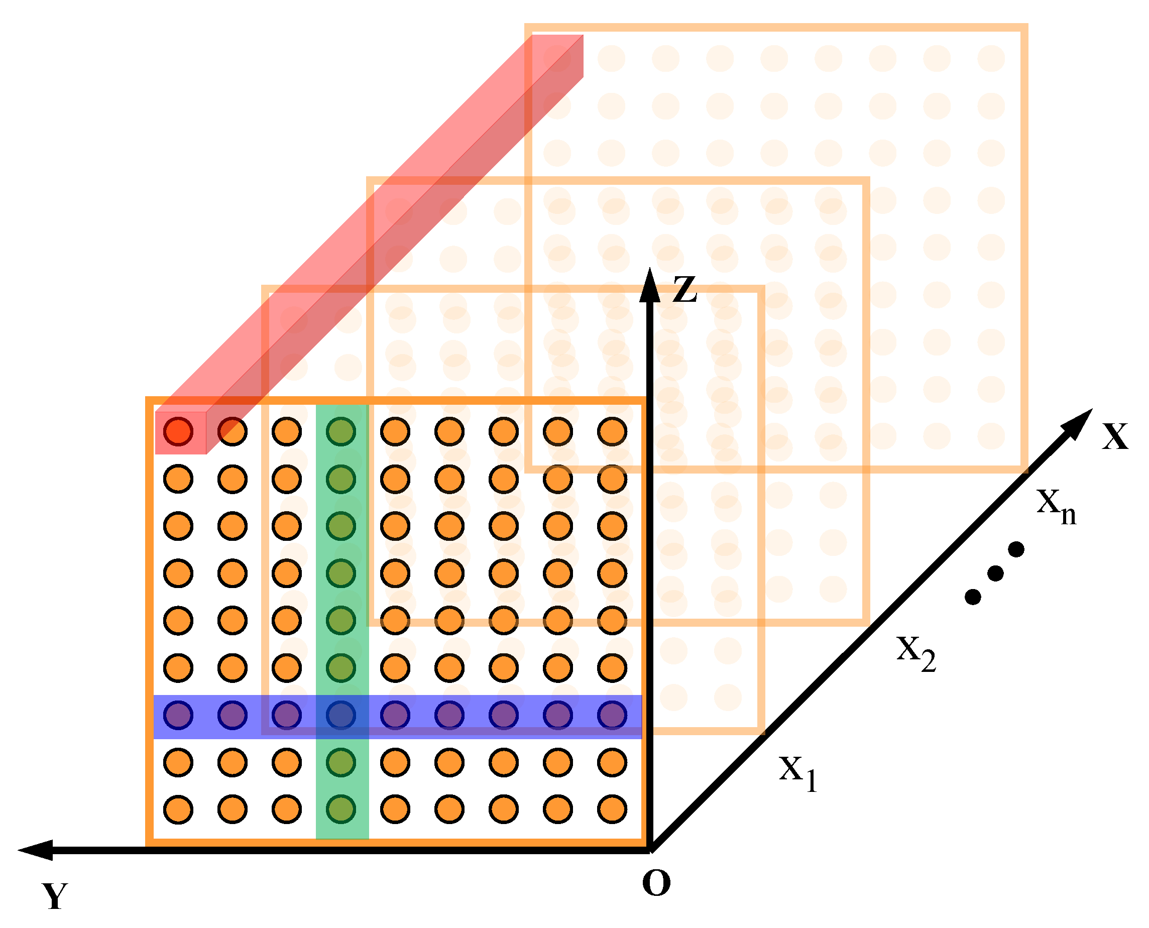
Figure 1. Schematic diagram of three-dimensional evidence source.
Machines 13 00868 g001
Figure 2. Visualization of traversable regions and distance field slices.
Machines 13 00868 g002
Figure 3. Mine roadway layout.
Machines 13 00868 g003
Figure 4. Experimental scenario.
Machines 13 00868 g004
Figure 5. Variation in dust filtration precision across different frame rates in various scenarios.
Machines 13 00868 g005
Figure 6. Risk assessment results for different scenarios of alleyway accessibility.
Machines 13 00868 g006
Table 1. Mine-DW-Fusion detection performance in different complex environments. Here, VN denotes the average voxel number; FP-I and FP-II represent the average number of filtered points in Stage I and Stage II, respectively; ACC-I and ACC-II denote the accuracy of Stage I and Stage II; and PG refers to the performance gain.
Scene VNFP-IFP-IIACC-I (%)ACC-II (%)PG (%)
Return entry391568727582.4992.9710.48
Return airway with person within 1 m25433966584.3897.4013.02
Return airway with person within 2 m279166814276.0194.8818.87
Main haulage roadway32991666895.2298.032.81
Upper-level yard25501635293.5797.974.40
Curve section in the upper yard28021233095.6198.923.32
Average298336710587.8896.78.82
Table 2. Experimental configuration and runtime.
ParameterValue
Bounding volume size 15 m × 10 m × 8 m (L × W × H)
Voxel resolution 0.1 m × 0.1 m × 0.1 m (L × W × H)
Maximum voxel count 1.2 × 10 6
Peak memory usage 82 MB
CPUi7-12700H
Risk-evaluation runtime 4.642 s
Table 3. Evaluation results of different methods in different scenarios. Here, RA = Return airway; RA-1m = Return airway with person within 1 m; RA-2m = Return airway with person within 2 m; MH = Main haulage roadway; ULY = Upper level yard; CS = Curve section in the upper yard. In addition, RDC denotes risk distribution continuity and RD denotes risk differentiation.
Method RARA-1mRA-2mMHULYCS
RDCRDRDCRDRDCRDRDCRDRDCRDRDCRD
D-S Theory0.8580.9150.8190.9160.8650.9150.8530.9160.8840.9140.8920.914
Averaging Method0.8510.8960.7880.9000.8470.8990.8370.9080.8700.8880.8790.893
Conservative Max0.8290.8960.8240.8960.7610.9020.7800.8960.8100.8860.8540.912
Bayesian0.7370.7410.7350.7580.8480.7530.8670.7560.7610.8560.8280.747
Entropy Weighted0.8510.8940.7950.8990.8480.8990.8370.9090.8700.8880.8810.886
Table 4. Overall evaluation performance of different methods in all scenarios.
MethodRisk Distribution ContinuityRisk Differentiation
MeanStdMeanStd
D-S Theory0.8618330.0258410.9150.000894
Averaging Method0.8453330.0320420.8973330.006802
Conservative Max0.8096670.0340390.8980.008579
Bayesian0.80550.0642890.7521670.007278
Entropy Weighted0.8470.030020.8958330.008424
Disclaimer/Publisher’s Note: The statements, opinions and data contained in all publications are solely those of the individual author(s) and contributor(s) and not of MDPI and/or the editor(s). MDPI and/or the editor(s) disclaim responsibility for any injury to people or property resulting from any ideas, methods, instructions or products referred to in the content.