Abstract
Leak detection in atmospheric vertical storage tanks is crucial for preventing environmental pollution, ensuring production safety, and reducing economic losses. This study investigates orifice leaks in vertical cylindrical storage tanks under atmospheric pressure using FLUENT 16.0. The simulation reveals a significant abrupt pressure change at the leak location. Based on the simulation findings, the actual acquired pressure signals during leakage are processed with wavelet threshold denoising, confirming the abrupt pressure change characteristic. Time-domain and waveform features of the denoised signals are extracted to establish a support vector machine (SVM)-based leak detection model. The performance of different kernel functions is compared, with the linear kernel achieving the highest accuracy of 96.55%.
1. Introduction
1.1. Background
The storage tanks used in the petrochemical industry are of diverse types. Based on their forms, they can be classified into vertical tanks, horizontal tanks, and special-structured tanks. In terms of applications, they cover tanks for storing raw materials, intermediate products, finished products, and waste materials. Regarding materials, they include both metallic and non-metallic tanks to meet the requirements of different media, pressures, temperatures, and storage scales [1,2]. Among them, atmospheric vertical cylindrical steel storage tanks are widely utilized, primarily for storing crude oil, refined oil products, and other liquid chemicals, with capacities ranging from several hundred to over one hundred thousand cubic meters [3]. These tanks are extensively applied in refineries, oil depots, and chemical industrial parks. Due to prolonged exposure to harsh environmental conditions, these tanks are susceptible to leaks caused by corrosion, material degradation, welding defects, or mechanical damage. According to statistics, tank leakage accidents occur frequently, with hundreds of cases reported globally each year. These incidents not only result in substantial economic losses but may also trigger severe consequences, such as fires, explosions, and environmental pollution [4]. Therefore, the development of efficient and accurate leakage detection technologies for oil storage tanks is of critical significance for ensuring safe production, minimizing resource wastage, and protecting the environment.
Currently, the evaluation of tank tightness is typically conducted through periodic inspection procedures, encompassing various approaches such as open-tank inspection and online detection. These assessment protocols are often carried out in accordance with national standards or industry specifications (e.g., API 653, GB 50341) during pre-commissioning, scheduled maintenance, or abnormal operational conditions. Commonly employed non-destructive testing (NDT) techniques for leakage detection include ultrasonic testing [5], magnetic flux leakage testing [6], infrared thermography [7], acoustic emission testing [8], optical fiber sensing [9], and resistive sensing, as well as manual inspections.
Ultrasonic testing identifies cracks or holes by analyzing the propagation characteristics of ultrasonic waves in tank walls, offering high accuracy but being susceptible to environmental noise interference and entailing high equipment costs [10]. Infrared thermography detects leaks by leveraging temperature differences between the leakage area and the surrounding environment, making it suitable for rapid, large-area scanning but less sensitive to minor leaks [11]. Acoustic emission technology locates leakage points by capturing elastic wave signals released during material fracture, yet it requires complex signal processing and is sensitive to background noise [12]. Additionally, resistive sensing cable systems enable real-time leakage monitoring and localization but rely on cable layout and the conductive properties of the medium [13]. Fiber-optic sensing technology achieves high-sensitivity monitoring by detecting optical signal changes induced by leaks, particularly suitable for flammable and explosive environments, but it is costly and prone to damage [14]. Manual inspections cannot guarantee real-time detection. Evidently, the aforementioned methods all exhibit certain limitations in atmospheric storage tank applications, underscoring the urgent need for the development of new detection techniques.
1.2. Related Work
In recent years, with the rapid advancement of artificial intelligence (AI) technologies, machine learning has demonstrated tremendous potential in industrial fault detection [15]. Machine learning methods can automatically extract leakage features from vast amounts of historical data and establish high-precision classification or regression models, thereby enhancing the real-time performance and accuracy of leakage detection [16]. Scholars worldwide have conducted extensive research in this field. He [17] analyzed leakage behavior in flammable liquid storage tanks under operational conditions and established a rapid-response detection model based on key leakage parameters. Kang [18] analyzed acoustic emission (AE) signals by examining AE parameters (e.g., frequency, amplitude, and RMS) as functions of angular and axial distances, proposing a mathematical model for orifice leakage-induced AE in cylindrical containers, thereby providing an accurate solution for leak source localization. Sohaib [19] extracted time-domain statistical features from acoustic emission signals of spherical tanks and utilized support vector machines (SVMs) to distinguish between intact and cracked states. Gorawski [20] designed a data analysis method incorporating expert knowledge to account for uncertainties and oscillations in data, generating stable trends for leak detection in time-series data. Mendoza [21] introduced a hydrocarbon-permeable coating doped with indicators as a cladding for glass/polymer optical fibers. Upon contact with fuel leaks, this coating alters the fiber’s spectral transmission characteristics, forming the basis of the HySense™ system for leak detection and localization. Rahimi [22] processed hydrophone sensor data using fast Fourier transform (FFT), wavelet transform, and time-domain features and then input the results into a 1D convolutional neural network (1D-CNN) for leak detection. The results demonstrated that FFT-based feature extraction outperformed other methods in detecting leaks in plastic and composite tanks. Despite advancements in leak detection technology, research on atmospheric storage tanks remains limited. This is primarily because their internal pressure remains at atmospheric pressure, causing changes in fluid dynamics during leaks to be too subtle for reliable detection.
With the advancement of Industrial Internet of Things (IIoT) technology, pressure signal-based leak detection methods for storage tanks have gradually shifted from traditional threshold-based approaches to data-driven intelligent diagnostics [23,24,25]. As a core technology in this field, machine learning can automatically extract potential fault patterns from high-dimensional signal features, demonstrating significant advantages in small-sample and nonlinear scenarios. Compared with conventional statistical analysis methods, machine learning models effectively address pattern confusion caused by noise interference and operational fluctuations in pressure signals through feature space mapping [26]. Support vector machine (SVM), a classic supervised learning algorithm proposed by Vapnik in 1995, is grounded in the idea of using kernel functions to map low-dimensional nonlinear separable samples into high-dimensional feature spaces, where an optimal hyperplane is constructed for classification [27]. In fault detection, SVM offers three key advantages: (1) the principle of structural risk minimization ensures generalization capability under small-sample conditions; (2) the kernel trick enables flexible handling of nonlinear feature relationships; and (3) its convex optimization property avoids the local optimum issues common in neural networks [28].
In fault diagnosis, SVM can accurately identify mechanical wear, electrical anomalies, and other fault types by analyzing equipment vibration, temperature, or current signals [29,30]. For pipeline leak detection, SVM integrates pressure, flow rate, and acoustic signal data to establish high-precision classification models, enabling timely leak localization and reduced false alarms [31,32]. To address this gap, this study proposes an orifice leak detection method for atmospheric vertical cylindrical storage tanks using pressure signals. A comparative analysis of the implementation costs between the proposed method and the aforementioned techniques is presented in Table 1.

Table 1.
Cost comparison of leak detection methodologies.
2. Numerical Simulation of Orifice Leakage Using FLUENT
2.1. Fluid Parameter Settings and Basic Assumptions
Numerical simulation of the orifice leakage process in atmospheric vertical cylindrical storage tanks was conducted using FLUENT 16.0 to investigate the pressure variation characteristics at the leakage orifice. Numerical simulation through computational fluid dynamics (CFD) enables precise capture of transient pressure distributions and vortex structure evolution in leakage flows, effectively overcoming the limitations of conventional experimental methods, including high costs, significant safety risks, and challenges in parametric analysis [33].
The present simulation employs water as the experimental medium, primarily based on the following considerations:
- Water is non-toxic, non-flammable, easily accessible, and simple to handle, which significantly reduces safety risks and operational costs during practical experimental stages, making it particularly suitable for initial method validation and repetitive testing.
- Different oil products (such as crude oil, gasoline, and diesel) exhibit variations in transient leakage responses (e.g., amplitude and frequency) due to their distinct physical properties, like viscosity and density. Using water as the medium helps isolate the interference caused by the complex physical characteristics of specific oil products during the principal exploration phase.
The core principle lies in analyzing and capturing the characteristic pressure transient changes (or pressure pulsations) driven by pressure differences and inertia during leakage, which is a universal hydrodynamic phenomenon in Newtonian fluids. Therefore, although the experiment is conducted in a water storage tank system, the method possesses a theoretical basis for extension to other sealed or pressurized liquid storage and transportation equipment, provided that leakage can induce measurable pressure fluctuations at the monitoring point.
Under ambient temperature conditions, the material properties of water and air are provided in Table 2. The simulation was based on the following fundamental assumptions:
Table 2.
Physical properties of water and air.
- The leakage orifice diameter remains constant throughout the leakage process, with no deformation caused by fluid–structure interaction or corrosion effects;
- Gravitational acceleration remains unchanged during the leakage, excluding seismic or inertial disturbances;
- Both water and air are treated as ideal substances without undergoing physical changes;
- The environmental temperature and the temperatures of water and air maintain their initial values during the simulation.
2.2. Simulation Experiment
The leakage model of the oil tank orifice studied in this paper is axisymmetric. Therefore, only half of the computational domain needs to be simulated for analysis, as shown in Figure 1a.
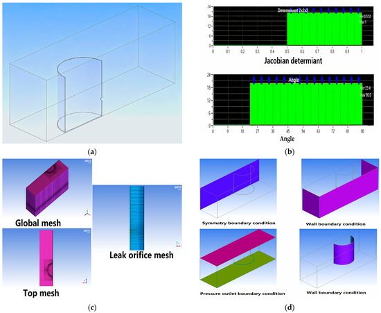
Figure 1.
FLUENT simulation process. (a) Computational domain; (b) mesh quality assessment; (c) computational domain mesh; (d) boundary conditions.
Setting appropriate mesh parameters is essential to achieve a suitable number of grid elements, proper sizing, and high-precision computational results. Excessive grid elements can significantly increase computation time, while too few may fail to fully capture the characteristics of the flow field. After repeated trials, the maximum grid size adopted in this study was ultimately set to 0.04 m. Additionally, grid refinement was applied to the tank wall and leakage hole by specifying the number of nodes on the boundaries. The resulting mesh quality is illustrated in Figure 1b. The total number of grids in the model is 277,261. Figure 1c shows the grid result of the computational domain.
The symmetry boundary condition was applied, which requires no specific boundary settings on the symmetric plane. On this plane, the normal velocity is zero, and the normal gradients of all variables also vanish. A pressure outlet boundary condition was adopted at the exit. All surfaces of the oil tank, along with the other three sides, were set as no-slip wall conditions. The boundaries defined in the computational domain established in this study are illustrated in Figure 1d.
The numerical simulation of orifice leakage phenomena in the vertical cylindrical storage tank was performed using FLUENT.16.0 computational fluid dynamics software, as depicted in Figure 1a–d. The geometrical parameters of both the storage tank and its computational domain are detailed in Table 3. The solution domain was discretized using structured hexahedral grids, with particular mesh refinement applied to critical regions including the tank wall surfaces and leakage orifices. Appropriate boundary conditions were subsequently assigned to complete the numerical model setup. Pressure monitoring points were positioned at the leakage orifice (Figure 2).
Table 3.
Numerical simulation dimensions.
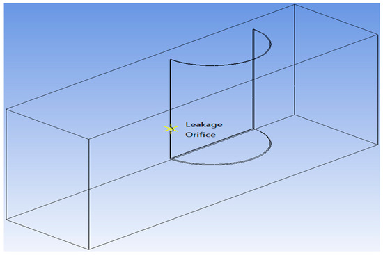
Figure 2.
Monitoring point locations.
The ambient pressure was set to the standard atmospheric pressure of , with a gravitational acceleration of and an ambient air density of . The reference pressure location was fixed at (0.3, 0.5, 1.4) within the computational domain, a position always occupied by the air phase. The initial liquid level in the oil tank was set to. A time step size ofwas adopted, with result files saved every 250 steps. The total number of iteration steps was 5000, corresponding to a simulated physical time of 10 s for capturing the pressure variation during the leakage process.
2.3. Simulation Results and Analysis
The computational results of the flow field were analyzed according to requirements. The pressure contour plot of the flow field is shown in Figure 3.
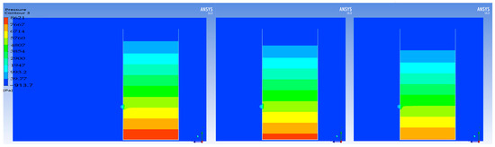
Figure 3.
Pressure contour on the symmetry plane at 1 s, 5 s, and 10 s of leakage.
As can be seen in Figure 3, the pressure in the simulation exhibits a gradient variation consistent with hydrostatics, demonstrating the validity of the simulation results.
Based on the hydrodynamic analysis of the tank leakage derived from Figure 4, the pressure variation on the horizontal plane at the same height as the leakage orifice is given by Equation (1). A comparison between the calculated and simulated hydraulic pressure changes on this plane, as shown in Figure 5, reveals that both exhibit consistent trends, indicating strong agreement between the mathematical model and numerical simulation of the oil tank leakage. The calculated hydraulic pressure remains approximately 60 Pa higher than the simulated values throughout the process, which is attributed to the presence of the gas–liquid interface during the simulation.
where represents the initial height from the leakage hole to the liquid surface; denotes the real-time height from the leakage hole to the liquid surface; indicates the internal pressure of the oil storage tank through which liquid flows out solely under the influence of gravity; is discharge coefficient; is the leakage orifice cross-sectional area; is cross-sectional area of the oil storage tank; denotes the density of water; and represents the gravitational acceleration.
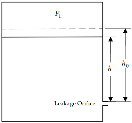
Figure 4.
Simplified diagram of tank dimensions.
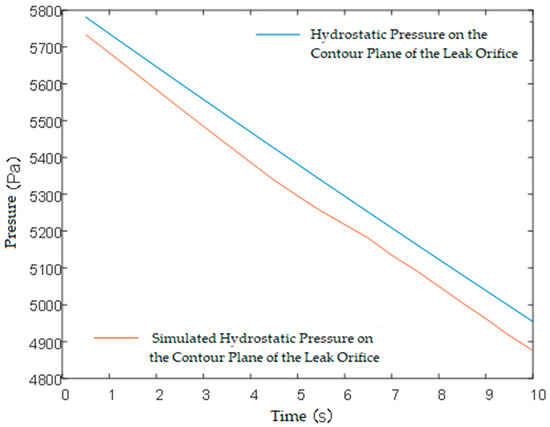
Figure 5.
Hydrostatic pressure on the contour plane of the leakage orifice.
Figure 6 shows the simulated pressure at the leakage orifice within 10 s of leakage. During the initial transient phase following the opening of the leakage orifice, the fluid inside the tank must overcome its inherent inertia to accelerate from a stationary state. To drive the entire fluid system toward the leakage point and establish a stable flow field, an additional pressure gradient must be provided to supply the accelerating force, which manifests as an initial rise in local pressure near the leakage orifice. This process lasts approximately 2.5 s. Once the flow is fully developed and reaches a quasi-steady state, the pressure energy is primarily converted into fluid kinetic energy and used to overcome viscous dissipation, causing the pressure at the leakage orifice to subsequently decrease and stabilize.
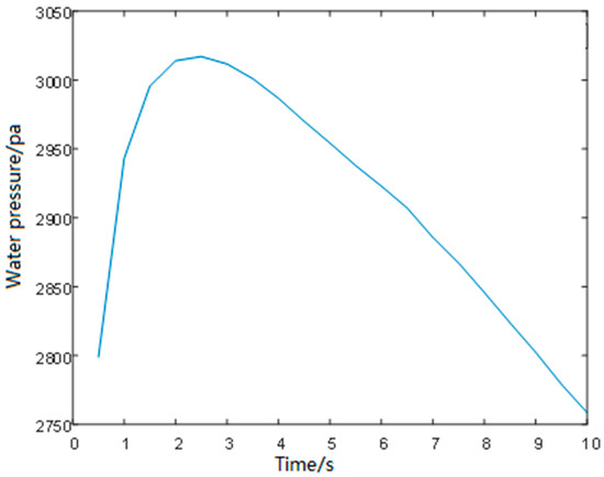
Figure 6.
Simulated water pressure variation at the leakage orifice.
The simulation results indicate that the pressure at the leakage orifice exhibits a trend of initial significant increase followed by a decrease, reaching its peak at 2.5 s. Due to the incompressibility of the liquid and the pressure wave propagation effect, slight fluctuations in pressure are also observed in other regions of the storage tank, rather than a smooth gradient decline. Therefore, pressure transmitters can be installed on the tank to utilize pressure signals as characteristic features for leakage detection.
3. Signal Analysis and Characteristic Parameter Extraction
3.1. Hydraulic Pressure Signal Processing
The simulated storage tank has an inner diameter of , a height of , and a volume of approximately , with an internal water level maintained at . The complete experimental platform for orifice leakage simulation is shown in Figure 7. Signals were acquired by pressure transmitters installed at the bottom of the tank wall, with their specifications summarized in Table 4. Leakage Orifice 1, located farthest from the pressure transmitter, was selected for the experiment. The orifice is positioned above the bottom of the storage tank and has an inner diameter of . The sampling frequency was set to , and based on observed pressure signals during leakage, the number of sampling points per sample was determined to be .
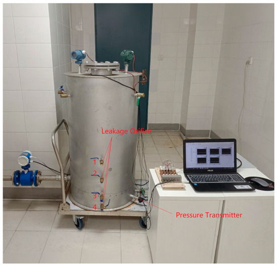
Figure 7.
Orifice leakage simulation platform for storage tanks.
Table 4.
Sensor parameters.
Pressure transducer signals are susceptible to random impulse noise interference (e.g., power fluctuations, equipment switching, etc.), which is characterized by high amplitude, short duration, and distinct outlier properties. The original water pressure signal, as shown in Figure 8, contains significant impulse noise. As a nonlinear method, median filtering proves highly efficient and robust in eliminating such impulse noise while minimally affecting the overall signal trend. This process provides a “clean” starting point for subsequent wavelet denoising. As shown in Figure 9, impulse noise is effectively removed after median filtering.
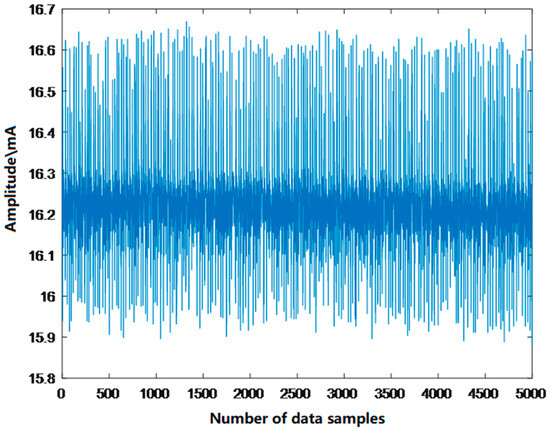
Figure 8.
Original hydraulic pressure signal.
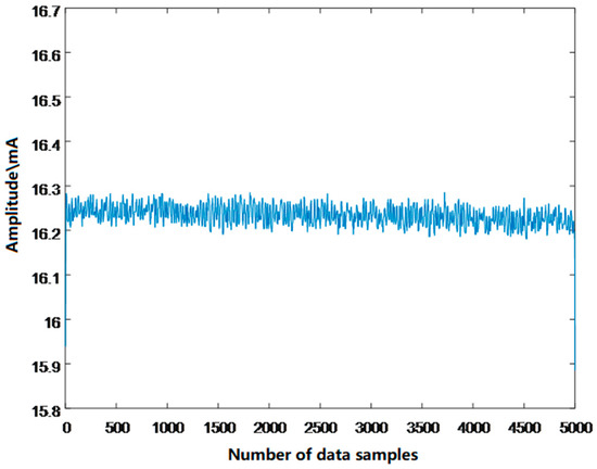
Figure 9.
Water pressure signal processed with median filtering.
3.1.1. Wavelet Threshold Denoising of Median-Filtered Water Pressure Signals
The median-filtered water pressure signals undergo wavelet threshold denoising. This process utilizes four distinct wavelet bases—Haar, Daubechies (db), Coiflets (coif), and Symlets (sym)—for signal decomposition. All decompositions maintain identical three-level decomposition scales, with Table 5 presenting the comparative results across different wavelet functions. The denoising effectiveness demonstrates an inverse relationship between the root mean square error (RMSE) and signal-to-noise ratio (SNR), where lower RMSE values correspond to higher SNR values, indicating superior noise reduction. For water pressure signals, the db6 wavelet basis achieves optimal denoising performance.
Table 5.
Performance comparison of different wavelet functions for hydraulic pressure signal denoising.
3.1.2. Multi-Level Wavelet Decomposition
The decomposition level significantly affects the denoising outcome. Excessive decomposition levels lead to substantial signal loss, while insufficient levels yield inadequate noise suppression [34]. Figure 10 presents the denoising results of water pressure signals processed with decomposition levels ranging from two to six. As shown in Figure 10b–d, the signals decomposed at levels 2, 3, and 4 still contain substantial noise. In contrast, the five-level wavelet decomposition yields superior results (Figure 10e), effectively removing a significant amount of noise while preserving most of the signal details. However, the signal becomes excessively smooth and distorted after six-level decomposition, as illustrated in Figure 10f. Therefore, the five-level wavelet decomposition was selected for signal processing.
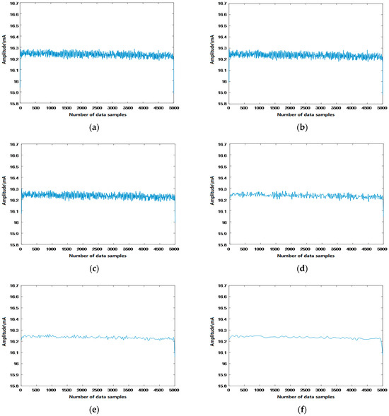
Figure 10.
Denoising performance across wavelet decomposition levels for hydraulic pressure signals. (a) Water pressure signal processed with median filtering; (b) Denoised water pressure signal after 2-level wavelet decomposition; (c) 3-level wavelet decomposition; (d) 4-level wavelet decomposition; (e) 5-level wavelet decomposition; (f) 6-level wavelet decomposition.
3.1.3. Denoising Threshold Optimization
Wavelet threshold denoising employs four threshold selection methods, as presented in Table 6, with the optimal predictor variable threshold demonstrating superior performance.
Table 6.
Threshold determination techniques for wavelet-based signal denoising.
Standard thresholding functions are compared in Figure 11, with mathematical formulations:
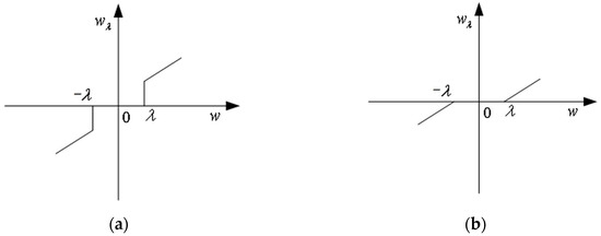
Figure 11.
Thresholding functions. (a) Hard thresholding functions; (b) soft thresholding functions.
- 1.
- Hard thresholding: see Equation (2).
- 2.
- Soft thresholding: see Equation (3).
The hard thresholding function yields a smaller root mean square error (RMSE) but introduces additional oscillations and discontinuities, resulting in poor smoothness. In contrast, the soft thresholding function produces wavelet coefficients with better continuity, eliminating spurious oscillations and demonstrating superior smoothness. Given the requirement for smooth variation trends in the acquired monitoring signals, the soft thresholding approach is adopted. As evidenced in Figure 12, the final denoised water pressure signal effectively removes interference noise while preserving useful components, achieving optimal performance.
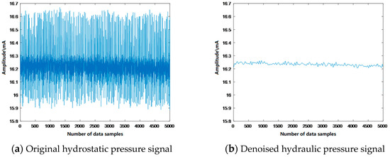
Figure 12.
Comparison of the original and denoised pressure signals.
The complete hydraulic pressure signal containing the leakage transient is acquired, as shown in Figure 13a. This pressure signal segment undergoes wavelet-based denoising, with the processed results demonstrated in Figure 13b.
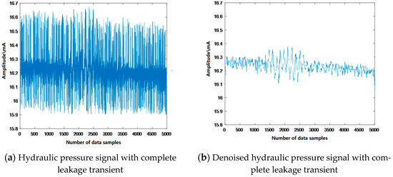
Figure 13.
Comparison of the original and denoised pressure signals with complete leakage transients.
3.2. Feature Selection
As shown in Figure 13, the hydraulic pressure signal exhibits marked differences between leakage and non-leakage conditions, with a distinct transient response of approximately 1500 sampling points (0.3 s) observed during leakage initiation. Comprehensive signal analysis reveals two categories of discriminative features:
- Time-domain characteristics, including mean, variance, standard deviation, energy, and average amplitude;
- Waveform parameters comprising skewness, kurtosis, impulse factor, and crest factor.
As quantitatively summarized in Table 7, these features collectively characterize the signal’s fluctuation magnitude (variance), distribution asymmetry (skewness), peak sharpness (kurtosis), and dynamic range (peak-to-peak value), with each 5000-point (1 s) data segment providing sufficient resolution for reliable leakage detection while maintaining computational efficiency for real-time monitoring applications.
Table 7.
Key parameters for leakage identification.
Hydrostatic pressure signals from oil storage tanks were analyzed to detect leakage conditions. Twenty samples were collected for both the leakage and non-leakage conditions. Five statistical features—variance, standard deviation, skewness, kurtosis, and peak-to-peak (P-P) amplitude—were calculated for each sample. The comparative results of these features are presented in Figure 14, while the mean values of the features are summarized in Table 8. The normalized feature values shown in the figure all range below 1. Each sample contains five characteristic features. The results demonstrate that these five features exhibit excellent discriminative capability for leakage detection.
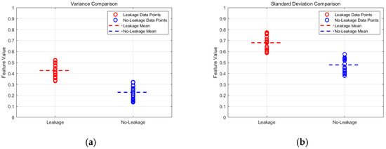
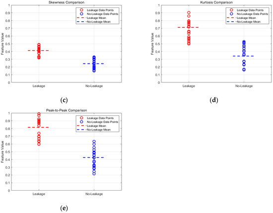
Figure 14.
Comparative analysis of feature values between 20 leak and no-leak conditions. (a) Variance comparison; (b) standard deviation comparison; (c) skewness comparison; (d) kurtosis comparison; (e) peak-to-peak value comparison.
Table 8.
Comparative analysis of mean feature values across 20 leak/no-leak conditions.
4. Experiment and Analysis
4.1. Orifice Leakage Detection Experiment
The leakage detection pipeline for storage tanks comprises the following steps:
- Signal Acquisition: Utilizing an orifice leakage simulation platform, hydraulic pressure signals are acquired from fixed-position sensors installed on the tank wall under both intact and leakage conditions.
- Signal Processing and Feature Extraction: The raw pressure signals are first denoised through median filtering and wavelet thresholding and then analyzed to extract both time-domain features (mean, variance, peak-to-peak value) and waveform characteristics (skewness, kurtosis, crest factor) for leakage detection.
- Dataset Construction and Kernel Selection: A balanced dataset of 600 samples (300 leakage/300 non-leakage) is normalized to [0, 1] and partitioned into training/test sets. Binary classification labels are assigned (1: leakage, 0: non-leakage). Comparative evaluation of SVM kernel functions (linear, RBF, polynomial, Sigmoid) yields the optimal kernel based on accuracy.
- Hyperparameter Optimization: Cross-validation is employed to determine the optimal kernel parameters and penalty factor for the model.
- Data Stratification and Model Validation: Model performance is evaluated through both random partitioning (50% training/test split, n = 300 each) and stratified sampling (ensuring class balance), with final model selection based on comparative accuracy analysis.
By randomly dividing the acquired 600 samples (300 leakage samples and 300 non-leakage samples) into training and test sets of equal size (300 samples each and consisting of both leakage and non-leakage cases, with no requirement for equal distribution between the leakage sample and the non-leakage sample), the random partitioning was repeated 20 times. The proposed model employs the following metrics to evaluate its accuracy, as expressed in Equation (3).
where TP (True Positive) denotes the number of samples correctly predicted as positive, FN (False Negative) represents the number of positive samples incorrectly predicted as negative, FP (False Positive) indicates the number of negative samples erroneously predicted as positive, and TN (True Negative) corresponds to the number of samples correctly predicted as negative.
Different kernel functions were applied to detect the presence or absence of storage tank leaks. Figure 15 displays the confusion matrix for one of the test datasets, with predicted labels on the horizontal axis and true labels on the vertical axis. Based on the confusion matrix results, it is evident that the linear kernel-based SVM model demonstrates superior performance. The test set results from 20 trials are presented in Table 9.
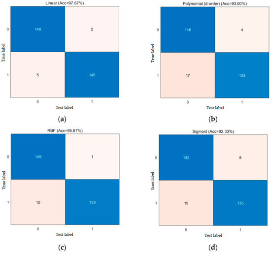
Figure 15.
Confusion matrices of different kernel functions. (a) Linear; (b) polynomial (d-order); (c) RBF; (d) sigmoid.
Table 9.
Performance comparison of different kernel functions in detection.
The experimental procedure involves randomly selecting two samples from the dataset at each iteration—one sample representing a leaking storage tank condition and the other representing a non-leaking condition—with the entire collection of 600 samples (comprising 300 leakage cases and 300 non-leakage cases) being partitioned into balanced training and test sets of equal size (300 samples each; the training set consists of 150 leakage samples and 150 non-leakage samples, and the test set follows the same composition). For robust evaluation, both balanced and randomized sample sets were repeatedly partitioned 20 times. Linear kernel SVMs were subsequently employed to perform leak detection (leak/no-leak classification) in storage tanks for each sample set variant. Table 10 presents the mean accuracy rates and mean AUC values across all 20 iterations, while Figure 16 displays a representative ROC curve from one trial, providing a comparison of the detection results between the different sample sets.
Table 10.
Performance comparison between the balanced and randomized sample sets.
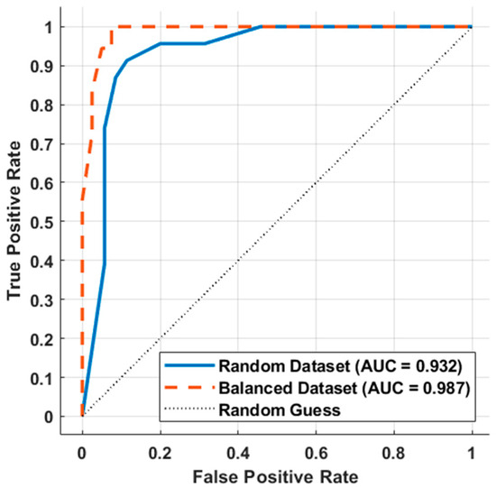
Figure 16.
ROC curves of models trained on different sample sets.
4.2. Results Analysis
The experimental results demonstrate that the linear kernel function achieved the highest leak detection accuracy of 96.55% across 20 test sets, outperforming other kernel functions, as shown in Table 9. Figure 14 further confirms its consistent superior performance in all test iterations, leading to its selection as the optimal kernel for our SVM-based oil storage tank leak detection system. Moreover, the implementation of sample balancing techniques significantly enhanced model performance, yielding a remarkable 97.00% average accuracy and 0.98 AUC value in the test sets (Table 10), which not only represents a 0.45% accuracy improvement over imbalanced data but also demonstrates more robust detection capability through the higher AUC score, with statistical significance confirmed by the t-test results (p < 0.01).
5. Conclusions
Numerical simulations in FLUENT verified the feasibility of using pressure signals for tank leakage detection. Raw signals were denoised via five-level Daubechies (db) wavelet decomposition. Key statistical features—variance, standard deviation, skewness, kurtosis, and peak-to-peak amplitude—were then extracted for leak/non-leak classification. Comparative analysis of SVM classifiers with linear, d-order polynomial, RBF, and sigmoid kernels showed the linear kernel performed best. Using a 1:1 train–test split under both random and balanced sampling, the SVM model with a linear kernel on balanced data achieved optimal overall performance.
Author Contributions
Conceptualization, G.Z.; methodology, G.Z. and F.C.; validation, F.C.; formal analysis, F.C. and X.L.; investigation, X.L. and F.L.; data curation, F.L.; writing—original draft preparation, J.Y.; writing—review and editing, G.Z.; visualization, X.L. and F.C.; supervision, G.Z.; project administration, J.Y.; funding acquisition, J.Y. All authors have read and agreed to the published version of the manuscript.
Funding
This work was supported by the Talent Program of the State Administration for Market Regulation (QNBJ202319), Research Projects of the State Administration for Market Regulation (2023MK070), and Projects of Fujian University Industry–Academic Cooperation (2022H6016).
Institutional Review Board Statement
This study did not involve humans or animals.
Informed Consent Statement
Not applicable.
Data Availability Statement
Due to the commercially confidential nature of these data, they cannot be made publicly available. The datasets supporting the findings of this study may be provided by the corresponding author upon reasonable request, subject to confidentiality agreements.
Acknowledgments
The authors gratefully acknowledge the valuable contributions of all researchers cited in this work, whose foundational studies made this research possible.
Conflicts of Interest
The authors declare no conflicts of interest.
References
- Rouzbahani, A.; Amirsradari, S.; Goudarzi, M. Experimental study of using an innovative porous floating roof for suppression of sloshing effects in cylindrical storage tanks. Ocean Eng. 2024, 310, 118735. [Google Scholar] [CrossRef]
- Salem, T.N.; El-Zohairy, A.; Abdelbaset, A.M. The Static and Dynamic Behavior of Steel Storage Tanks over Different Types of Clay Soil. Civil Eng. 2023, 4, 1169–1181. [Google Scholar] [CrossRef]
- Guan, W.H.; Tao, Y.H.; Cheng, H.Y.; Ma, C.J.; Guo, P.J. Present Status of Inspection Technology and Standards for Large-Sized In-Service Vertical Storage Tanks. In Proceedings of the ASME Pressure Vessels and Piping Conference, Baltimore, MD, USA, 17–21 July 2011; pp. 749–754. [Google Scholar]
- Li, X.; Chen, G.; Amyotte, P.; Alauddin, M.; Khan, F. Modeling and analysis of domino effect in petrochemical storage tank farms under the synergistic effect of explosion and fire. Process Saf. Environ. Prot. 2023, 176, 706–715. [Google Scholar] [CrossRef]
- Xue, H.; Wu, D.; Wang, Y.P.; Zhao, Z.N.; Chen, T.F.; Teng, Y.P. Research on ultrasonic leak detection methods of fuel tank. In Proceedings of the IEEE International Ultrasonics Symposium (IUS), Taipei, Taiwan, 21–24 October 2015. [Google Scholar]
- Pullen, A.L.; Charlton, P.C.; Pearson, N.R.; Whitehead, N.J. Magnetic Flux Leakage Scanning Velocities for Tank Floor Inspection. IEEE Trans. Magn. 2018, 54, 8. [Google Scholar] [CrossRef]
- Manekiya, M.H.; Arulmozhivarman, P. Leakage Detection and Estimation using IR Thermography. In Proceedings of the IEEE International Conference on Communication and Signal Processing (ICCSP), Melmaruvathur, India, 6–8 April 2016; pp. 1516–1519. [Google Scholar]
- Sun, L.Y.; Li, Y.B. Large Vertical Storage Tank Bottom Evaluation via Acoustic Emission Signal Analysis. In Proceedings of the 23rd Chinese Control and Decision Conference, Mianyang, China, 23–25 May 2011; pp. 3554–3558. [Google Scholar]
- Shang, Y.; Wang, C. Review of Distributed Optical Fiber Sensing Technology. J. Appl. Sci. 2021, 39, 843–857. [Google Scholar]
- Jiang, H.F.; Shen, Y.F.; Qu, Y.G. Damage detection and imaging for composite storage tanks utilizing ultrasonic guided waves. In Proceedings of the 2024 International Mechanical Engineering Congress and Exposition-IMECE, Portland, OR, USA, 17–21 November 2024. [Google Scholar]
- Shi, J.H.; Chang, Y.J.; Xu, C.H.; Khan, F.; Chen, G.M.; Li, C.K. Real-time leak detection using an infrared camera and Faster R-CNN technique. Comput. Chem. Eng. 2020, 135, 11. [Google Scholar] [CrossRef]
- Hu, Z.Y.; Tariq, S.; Zayed, T. A comprehensive review of acoustic based leak localization method in pressurized pipelines. Mech. Syst. Signal Proc. 2021, 161, 17. [Google Scholar] [CrossRef]
- Luo, K.W.; Shui, A.S.; Li, S.L.; Li, Z.Y.; Chen, J.C. Sensor Cable-Based Tank Leak Detection System. In Proceedings of the 23rd Chinese Control and Decision Conference, Mianyang, China, 23–25 May 2011; pp. 1320–1324. [Google Scholar]
- Su, C.Y.; Yang, S.R. Application of Optical Fiber Sensing Technology in Oil Tank Level Measurement. In Proceedings of the 7th International Conference on Advanced Design and Manufacturing Engineering (ICADME), Shenzhen, China, 10–11 May 2017; pp. 149–152. [Google Scholar]
- Asutkar, S.; Tallur, S. An explainable unsupervised learning framework for scalable machine fault detection in Industry 4.0. Meas. Sci. Technol. 2023, 34, 17. [Google Scholar] [CrossRef]
- Rizk, M.; Chehade, A. Efficient Oil Tank Detection Using Deep Learning: A Novel Dataset and Deployment on Edge Devices. IEEE Access 2024, 12, 170346–170378. [Google Scholar] [CrossRef]
- He, J.; Yang, L.; Ma, Y.; Yang, D.; Li, A.; Huang, L.; Zhan, Y. Simulation and application of a detecting rapid response model for the leakage of flammable liquid storage tank. Process Saf. Environ. Prot. 2020, 141, 390–401. [Google Scholar] [CrossRef]
- Kang, J.G.; Kim, K.B.; Koh, K.H.; Kim, B.K. Analytical Model and Gas Leak Source Localization Based on Acoustic Emission for Cylindrical Storage. Appl. Sci. 2025, 15, 5072. [Google Scholar] [CrossRef]
- Sohaib, M.; Islam, M.; Kim, J.; Jeon, D.C.; Kim, J.M. Leakage Detection of a Spherical Water Storage Tank in a Chemical Industry Using Acoustic Emissions. Appl. Sci. 2019, 9, 196. [Google Scholar] [CrossRef]
- Gorawski, M.; Gorawska, A.; Pasterak, K. The TUBE algorithm: Discovering trends in time series for the early detection of fuel leaks from underground storage tanks. Expert Syst. Appl. 2017, 90, 356–373. [Google Scholar] [CrossRef]
- Mendoza, E.; Kempen, C.; Esterkin, Y.; Sun, S.J. Fiber Optic Distributed Chemical Sensor for the Real Time Detection of Hydrocarbon Fuel Leaks. In Proceedings of the 24th International Conference on Optical Fibre Sensors (OFS), Curitiba, Brazil, 28 September–2 October 2015. [Google Scholar]
- Rahimi, M.; Alghassi, A.; Ahsan, M.; Haider, J. Deep Learning Model for Industrial Leakage Detection Using Acoustic Emission Signal. Informatics 2020, 7, 49. [Google Scholar] [CrossRef]
- Glentis, G.-O.; Georgoulaki, K.; Angelopoulos, K. Leak detection in the pipeline network of an oil refinery—A pattern classification paradigm. In Proceedings of the 24th Pan-Hellenic Conference on Informatics, Athens, Greece, 20–22 November 2021; pp. 178–182. [Google Scholar]
- Sun, J.; Xiao, Q.; Wen, J.; Zhang, Y. Natural gas pipeline leak aperture identification and location based on local mean decomposition analysis. Measurement 2016, 79, 147–157. [Google Scholar] [CrossRef]
- Gao, J.; Zheng, Y.; Ni, K.; Zhang, H.; Hao, B.; Yan, J. Research on oil-gas Pipeline Leakage Detection Method Based on Particle Swarm Optimization Algorithm Optimized Support Vector Machine. J. Phys. Conf. Ser. 2021, 2076, 012004. [Google Scholar] [CrossRef]
- Zhang, X.; Zhao, B.Y.; Lin, Y. Machine Learning Based Bearing Fault Diagnosis Using the Case Western Reserve University Data: A Review. IEEE Access 2021, 9, 155598–155608. [Google Scholar] [CrossRef]
- Huang, W.; Liu, H.; Zhang, Y.; Mi, R.; Tong, C.; Xiao, W.; Shuai, B. Railway dangerous goods transportation system risk identification: Comparisons among SVM, PSO-SVM, GA-SVM and GS-SVM. Appl. Soft Comput. 2021, 109, 107541. [Google Scholar] [CrossRef]
- Yin, S.; Gao, X.; Karimi, H.R.; Zhu, X.P. Study on Support Vector Machine-Based Fault Detection in Tennessee Eastman Process. Abstr. Appl. Anal. 2014, 8, 836895. [Google Scholar] [CrossRef]
- Guo, A.X.; Zhao, Z.; Sun, J.R.; Ge, H.Y. Fault classification of meta-action unit using CEEMDAN double-layer decomposition and COA-SVM. Syst. Sci. Control Eng. 2025, 13, 15. [Google Scholar] [CrossRef]
- Jonjo, E.R.; Ali, I.; Megahed, T.F.; Nassef, M.G.A. A Novel Framework for Motor Bearings Fault Diagnosis using a Heuristic based Adaptive Variational Mode Extraction and a Hybrid CNN-SVM Classifier of Current Signals. J. Vib. Eng. Technol. 2025, 13, 25. [Google Scholar] [CrossRef]
- Khalid, S.; Azad, M.M.; Kim, H.S. Real-World Steam Powerplant Boiler Tube Leakage Detection Using Hybrid Deep Learning. Mathematics 2024, 12, 3887. [Google Scholar] [CrossRef]
- Zhao, X.Y.; Zhang, Z.R.; Du, X.P.; Wang, Y.; Yang, J.C.; Feng, Z.J.; Zhong, R.Y.; Han, C.; Mo, J.X.; Wan, J.L.; et al. Study on the characteristics of vibration acoustic signals and rupture grading for reactor pipeline leaks. Ann. Nucl. Energy 2025, 222, 11. [Google Scholar] [CrossRef]
- Cheng, W.P.; Shen, Y.X.; Xu, G. Experimental and numerical modeling of sidewall orifices. SN Appl. Sci. 2020, 2, 20. [Google Scholar] [CrossRef]
- Barsanti, R.J.; Gilmore, J. Comparing Noise Removal In The Wavelet And Fourier Domains. In Proceedings of the SSST 2011—43rd IEEE Southeastern Symposium on System Theory, Auburn, AL, USA, 14–16 March 2011; pp. 163–167. [Google Scholar]


Disclaimer/Publisher’s Note: The statements, opinions and data contained in all publications are solely those of the individual author(s) and contributor(s) and not of MDPI and/or the editor(s). MDPI and/or the editor(s) disclaim responsibility for any injury to people or property resulting from any ideas, methods, instructions or products referred to in the content. |
© 2025 by the authors. Licensee MDPI, Basel, Switzerland. This article is an open access article distributed under the terms and conditions of the Creative Commons Attribution (CC BY) license (https://creativecommons.org/licenses/by/4.0/).