Abstract
In modern manufacturing, achieving high-speed laser cutting requires advanced robotic trajectory planning for smoothness and collision avoidance. Poorly optimized motion can cause frequent velocity changes, leading to mechanical vibrations that shorten machine service life. This study presents an innovative trajectory optimization approach for laser cutting machines equipped with a redundant standoff axis. A B-spline-based analytical model formulates rotational axes trajectories as quadratic programming problems to minimize jerk (the rate of acceleration change) under machining accuracy and kinematic constraints. Additionally, an M path, represented by the wrist center’s trajectory, refines translational axes by adjusting the standoff axis through a similar optimization model, thereby reducing mechanical stress. Collision avoidance is ensured through a concurrent iterative optimization process, considering the feasible domains of representative 3D geometric tool orientations. Simulation experiments on a complex B-pillar workpiece demonstrate the framework’s effectiveness, clearly indicating significant reductions in jerk and improved trajectory smoothness for both rotational and translational axes compared with conventional methods and a prior approach. This work advances high-speed machining capabilities by offering a novel, robust solution that leverages redundant structures to further improve trajectory smoothness and reliability in demanding industrial applications.
1. Introduction
High-speed and high-precision manufacturing applications, especially in 3D laser cutting manufacturing (LCM) [1], demand trajectory optimization strategies that not only achieve efficiency and accuracy, but also maintain collision-free operations. Leveraging redundancy to enhance smoothness is paramount since abrupt changes in the machining path can induce vibrations, degrade part quality, and intensify mechanical stress and wear [2]. Although modern five-axis CNC machines provide advanced motion-control capabilities, the full integration of minimized-jerk methods with the simultaneous optimization of both tool orientation and translational axes remains a significant challenge, yet it is essential for maximizing performance in 3D LCM tasks.
Conventional five-axis laser cutting machines often struggle to maintain smooth movement, especially when dealing with inertia effects and rapid axis accelerations in complex machining regions. These difficulties stem not only from the mechanical limitations of traditional systems, but also from the computational burden of planning optimal, interference-free tool paths. Existing studies frequently place an excessive focus on optimizing the two rotational axes through tool orientation adjustments for smoothness and collision avoidance. However, the significance of the three translational axes’ motion is often underestimated, even though optimizing it is equally crucial for improving overall machining accuracy, reducing dynamic stress, and enhancing the trajectory’s smoothness.
1.1. Related Works
Numerous studies on tool orientation adjustment in five-axis machining focus on identifying discrete interference-free regions. They also aim to prevent vibrations caused by abrupt changes between adjacent cutter location (CL) points in the rotational axes. Initially, many of these works [3,4,5] demonstrated that smoother tool orientation transitions along the tool path within the workpiece coordinate system (WCS) lead to improved trajectories. For example, Ho et al. [3] proposed to represent the orientation of the tool using quaternions and applied a smooth interpolation between the representative directions of the tool axis in the WCS. Lauwers et al. [4] developed a method to evaluate potential collisions and to incrementally adjust tool orientation using inclination and screw angles. Jun et al. [5] developed a search algorithm to minimize machined surface errors in machining of the five-axis sculptured surface. The algorithm determines local optimal tool orientations in the configuration space (C-space) in both forward and backward directions.
However, it was later recognized that planning tool orientations solely within the WCS does not necessarily guarantee smooth rotational axis movements. This is due to the nonlinearity of the inverse kinematic transformation (IKT) used to convert from the WCS to the machine coordinate system (MCS) in a five-axis machine structure [6].
The kinematic performance of the rotational axes can be further enhanced when optimization is performed directly in the MCS, according to Castagnetti et al. [7]. In their work, the feasible domain of tool orientation, known as the domain of admissible orientation (DAO), was defined through four linear inequality constraints. This was achieved using a gradient-based optimization model.
This initial attempt to smooth the rotational axis movements directly in the MCS inspired the development of many smoothing algorithms [2,8,9,10,11]. These methods focused on avoiding gouging and collisions along the tool path while enhancing rotational axis motion in five-axis machining. Wang et al. [9] represented the nonlinear kinematic constraints and the irregular geometric feasible domain (GFD) using a linearization strategy, which allowed the optimization problem to be solved using simple linear programming. Plakhotnik and Lauwers [10] proposed a graph-based method that utilized Dijkstra’s algorithm to find the shortest path for rotational axis transitions between two adjacent admissible arcs. Xu et al. [12] modeled the kinetic and frictional consumption of the rotational axes on a 3D laser cutting head. They constructed a graph with four combinations of the two rotational axes along discrete tool orientations to search for the shortest path, but the feasible regions are not analyzed. Building on the work of Plakhotnik and Lauwers [10], Mi et al. [11] improved rotational dynamics by incorporating an angular acceleration penalty component into a differential graph.
Most of the aforementioned methods determine the rotational joint coordinates along the continuous tool path using discrete points. Recent research suggests that the use of higher-order differentiable mathematical expressions, such as polynomials [7] or B-splines [13,14,15], offer better control and smoothness to generate tool orientation trajectories. Huang et al. [16] employed radial basis functions to construct the tool orientation field. Xu et al. [13] developed an iterative representative tool orientation (RTO)-based method to generate a continuous rotational axis trajectory, represented using a B-spline curve in the MCS. The method checks for interference along the entire tool path and iteratively inserts additional RTOs as needed. This approach helps to decouple geometric and kinematic constraints during the tool orientation process. Xiao et al. [14] minimized sudden changes in tool orientation by incorporating contour error prediction constraints. Wu et al. [15] formulated a quadratic programming (QP) problem to compute jerk-optimal B-spline coefficients, with linear constraints derived from kinematic limits and geometric constraints based on the GFD. Their experiments showed enhanced machining stability and surface quality compared to the quaternion interpolation (QI) and angular-acceleration optimal methods.
An alternative method [17] to determine the smooth tool orientation involves synchronized interpolation using dual NURBS curves. Yuen et al. [18] achieved smoothness trajectories, improving the machining accuracy by minimizing the geometrical jerk. Li et al. [19] incorporated machining error considerations into the dual spline method.
Significant advancements have been made in smoothing tool orientation through various methodologies. Another promising approach to improve trajectory smoothness in robotic systems is to use additional degrees of freedom. Additional degrees of freedom in redundant robotic systems allow trajectory planning and execution to be refined, achieving greater smoothness and precision. A promising redundancy strategy is known as macro–micro, which combines a macro-scale robot for large movements with a micro-scale robot for precision [20]. Enhancing dexterity and precision through redundancy, this configuration has been widely used in industries for manipulation [21], robotic machining [22,23], and medical surgery [24]. In laser cutting applications, which require speed and precision over large areas, the macro–micro structure is highly advantageous. Uzunoglu [25] optimized machining by distributing planar paths between primary x-y and secondary u-v mechanisms. Liu [26] demonstrated efficiency improvements using a velocity planning algorithm for macro and micro platforms. However, most laser cutting applications are limited to planar surfaces and lack consideration for complex 3D five-axis machining applications. In our previous work [27], we proposed a conic posture interpolation method to cut closed-contour holes with a “polar” robot on the laser head, achieving improved efficiency. Substantial opportunities remain to optimize trajectories by utilizing the macro–micro redundant structure in laser cutting applications.
1.2. Contributions
While significant advancements have been made in optimizing tool orientation and collision avoidance for five-axis machining, trajectory planning methods specifically targeting smoothness optimization along translational axes have received comparatively less attention. To address this gap, our prior work [28] introduced a two-step optimization approach, employing a graph-based algorithm for collision-free tool orientation planning, followed by reinforcement learning to optimize the redundant standoff axis. Although effective in specific scenarios, these methods were computationally expensive [10,12] due to the high dimensionality of the GFD required for graph construction and extensive collision checks. Additionally, numerical errors introduced by discrete differentiation methods in trajectory optimization increased substantially with higher-order derivatives, negatively impacting trajectory accuracy and smoothness.
To overcome these limitations, this work proposes a novel trajectory optimization strategy tailored specifically for 3D laser cutting machines equipped with a redundant standoff axis. The primary contribution of our research lies in developing an innovative optimization framework inspired by macro–micro structural approaches. This framework explicitly leverages the redundant axis to optimize translational axis trajectories jointly with tool orientations—an aspect rarely explored in the existing literature. A prototype of this machine, currently under development by EFORT Intelligent Robot Co., Ltd. (Wuhu, China), serves as the basis for our study (see schematic and axis definitions in Figure 1).
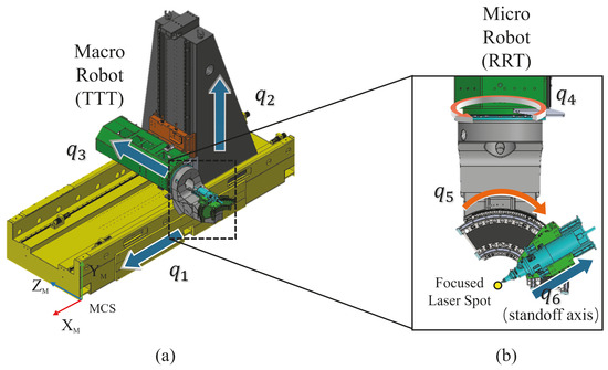
Figure 1.
The schematic of the EFORT 3D laser cutting machine. (a) Overall view, showing the macro robot (TTT) with three translational axes (T for translation). (b) Close-up of the micro robot (RRT), featuring the two rotational axes (R for rotation) and the redundant standoff axis .
Different from discrete graph-based methods, our proposed methodology uses an analytical joint trajectory model represented by B-splines, formulated explicitly as a QP problem. This analytical formulation significantly reduces computational complexity, avoiding numerical errors typically associated with high-order discrete differentiation. Moreover, by explicitly minimizing jerk instead of acceleration, the proposed minimized jerk trajectory optimization (MJTO) algorithm directly enhances smoothness by effectively mitigating abrupt changes in acceleration.
In addition, while existing iterative algorithms using RTO-based methods [3,13,15] often successfully find collision-free trajectories, they typically overlook optimizing initial RTO selections. Recognizing the critical impact of initial RTO configurations on trajectory quality, our study introduces a dedicated optimization process for strategically selecting initial RTOs. This dedicated selection process substantially improves trajectory smoothness, as well as the efficiency and effectiveness of the overall optimization.
Lastly, the high-speed, non-contact characteristics inherent in 3D laser cutting manufacturing frequently involve rapid and extensive tool orientation changes when machining complex geometries. Such large-angle and high-rate transitions impose substantial demands on trajectory smoothness and collision avoidance, challenges inadequately addressed by traditional methods. The MJTO approach developed herein specifically tackles these demanding conditions, ensuring smooth, jerk-minimized trajectories and reliable collision-free operations, thus effectively accommodating the challenging orientation variations that characterize advanced industrial laser cutting applications.
1.3. Structure of the Paper
This paper is organized into four sections. Section 2 introduces the minimized jerk trajectory optimization framework based on B-splines, first formulating a quadratic programming model to enhance the smoothness of joint trajectories, particularly for 3D laser cutting machines equipped with a redundant standoff axis. It then integrates an optimization RTO-based iterative procedure to ensure collision-free trajectory. Section 3 presents two illustrative case studies involving automotive B-pillar components, demonstrating significant improvements in trajectory smoothness and overall effectiveness compared with conventional methods and our earlier graph-based optimization approach. Finally, Section 4 summarizes the major contributions and suggests future research directions.
2. MJTO Methodology: Minimized Jerk Trajectory Optimization
This section introduces the proposed MJTO algorithm for 3D laser cutting machines equipped with a redundant standoff axis. The approach utilizes B-spline curves [13] to represent the joint displacement and ensure trajectory continuity and smoothness while expressing kinematic constraints [15]. Known as minimized jerk trajectory optimization, the method formulates the optimization problem as two QP tasks. A QP model based on B-splines is developed for the two rotational axes to minimize jerk, thereby enhancing trajectory smoothness and machining precision. Similarly, the redundant standoff axis is modeled within a QP framework to further smooth the rotational axes center point path, as referred to the M path in our previous work [28], and improve overall system performance. In addition, a collision avoidance strategy is introduced. It is based on the GFD in 3D joint space and an iterative RTO-based process. This ensures that the trajectory remains collision-free while satisfying kinematic constraints. The following subsections outline the key components of the MJTO methodology, including the mathematical representation of joint trajectories and M path using B-splines, the formulation of QP problems for rotational axes and the redundant axis, and the integration of collision avoidance mechanisms.
Firstly, this study builds on the trajectory representation framework developed in our previous work [28]. The laser head follows the CL point trajectory , which defines the tool path in Cartesian space, and the tool orientation , a unit vector representing the tool’s orientation direction. Both are defined in the workpiece coordinate system (WCS), as illustrated in Figure 2a. Here, the trajectories are parameterized using the normalized arc length parameter u, which is generated by a standard G-code interpolator with demanding machining parameters as
where denotes the arc length with respect to time t and is the total length of the tool path.
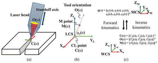
Figure 2.
(a) Laser head trajectory in the Local Coordinate System (LCS); (b) relationship between CL point, tool orientation, and M point in the LCS; (c) forward and inverse kinematic transformations between the Machine Coordinate System (MCS) and the Workpiece Coordinate System (WCS).
The concept of the second M point is introduced here, as shown in Figure 2b. This auxiliary point is used to characterize and enhance the smoothness of the primary translational axes during trajectory planning. Figure 2c illustrates the relationship between coordinate systems with respect to the joint coordinates defined as in Figure 1. The forward kinematic equations, which transform joint coordinates in MCS into WCS, are given by:
reversely, the conversion from WCS back to MCS, denoted as IKT, is formulated as
where the function determines the angle by considering the signs of and .
We note that u is not equivalent to the time variable t. The relationship between them is governed by the feedrate along the path and can be derived using (1) as
2.1. B-Spline Representation of Joint Space and Kinematic Constraints
The proposed MJTO algorithm uses B-spline curves to represent rotational axis displacement trajectories. Their smoothness and flexibility make them suitable for modeling complex trajectories, as they ensure continuity and differentiability up to a desired order [29]. Therefore, the displacement trajectories of the rotational axes , for , can be mathematically represented as
where are the B-spline basis functions of degree k, is the control coefficient, and is the number of the control coefficients.
The choice of degree of B-spline k determines the smoothness of the trajectory. A quintic B-spline () is typically chosen to ensure continuity since third-order differentiability helps to minimize abrupt changes in acceleration. The B-spline basis function can be derived recursively using a knot vector . A uniform method is employed for generating the knot vector, ensuring control points along the tool path. Consequently, the collection of control coefficients becomes the set of decision variables in (5), to be optimized in the jerk-minimization process.
Tool path interpolation is performed in the WCS, considering Cartesian tangential dynamic parameters with u. However, joint kinematic constraints are typically ignored during this stage, which can result in abrupt or non-smooth joint motions. Therefore, using the chain rule, the kinematic parameters of the joints, including angular velocity , angular acceleration , and angular jerk , are derived incorporating tangential dynamic parameters as
The kinematic parameters can then be reformulated using (4) as
where and represent the first and second deviates of feedrate with respect to time, respectively. Similarly, , , denote the first, second, and third geometricalderivatives of with respect to u. Hence, captures how the joint variable changes along the path from a purely geometric standpoint, whereas the feedrate describes how fast we traverse that path in time. The geometrical derivatives of the joint displacement are given below as
However, to impose linear constraints on the geometrical derivatives in terms of the design variable , we can reshape the geometrical derivatives in (8)–(10) in a general form for the r-th derivative, following De Boor’s algorithm for B-splines [15], as
where , is the interpolated node assigned on the CL point , and the geometrical derivative of the control coefficient can be computed recursively as
where are the control coefficients for the r-th geometric derivative of .
In many theoretical treatments, a constant feedrate (i.e., ) is assumed. This simplification is also adopted here to ease the parametric forms. However, in the application of practical machining, a variable value is assigned to feedrate, which is influenced by multiple factors, such as drive limitations, variations in machining trajectories, and specific manufacturing process requirements. In the current study, we assume a constant feedrate, as in [13,15,30], to highlight the core mechanisms of the minimized jerk method. Under this assumption, the kinematic parameters in (6) can be reformulated using (4) as
where we observe that the joint velocities, accelerations, and jerks are scaled by powers of the constant feedrate f.
To guarantee that the resulting trajectories remain within the feasible ranges of robot kinematics, we impose constraints on the rotational axes, including limits on angular velocity , acceleration , jerk , and the axis range . Owing to the convex hull property of B-spline curves, the resulting curve is guaranteed to lie entirely within the convex region defined by its control points. Therefore, by transferring the constant factor into the constraint formulation, the kinematic restrictions can be linearly expressed in terms of the control coefficients and their geometrical derivatives as
thus ensuring the desired bounds on velocities, accelerations, and jerks are not exceeded. These linearized constraints, together with the recursive relation in (12), provide a framework amenable to kinematic constraints using the B-spline representation. The subsequent section details how these constraints and objective functions are integrated into our proposed minimized jerk algorithm.
2.2. QP Minimized Jerk Modeling for Rotational Joint Trajectory Based on B-Spline
Achieving a smooth trajectory is crucial in high-precision 3D laser cutting applications, directly influencing the quality of the machining and the mechanical stress. Minimization of the jerk is an effective optimization objective, as it reduces abrupt motion changes, resulting in smoother tool movements [15,18].
Minimization of the jerk can be formulated as a QP problem subject to the kinematic constraints listed in (15). This ensures computational efficiency and guarantees the attainment of a global optimum due to the convexity of the QP, allowing efficient computation with standard solvers.
Therefore, the objective function for minimizing jerk on rotational axes can first be formally defined as the integral of squared jerk with respect to time over the total trajectory duration T as
By using the relationship between time t and the normalized arc-length parameter u given by (4), the integral domain can be transformed from the time domain to the parameter domain u. Incorporating (13) and assuming a constant feedrate f, (16) can be rewritten as
Defining the integral term as a scalar coefficient , which is nonzero only when , we have
Observing that the constant scaling factor does not influence the optimization search direction, we can safely omit this factor. Thus, by introducing the symmetric Hessian matrix with elements , the objective function can be compactly expressed in standard quadratic programming form with respect to the control coefficient vector as
The kinematic constraints outlined in (15) play a critical role in ensuring the feasibility of the trajectory and are incorporated into the QP problem as inequality constraints. Additionally, the states of kinematic parameters at and , corresponding to the initial and final trajectory conditions, must be enforced as equality constraints. These constraints ensure continuity and smooth transitions while adhering to specified boundary values, such as , , , and . The complete trajectory optimization problem is then expressed as a kinematic constrained QP problem, formulated as
As discussed in (12), linearization and recursive computation of control coefficients are crucial for optimization modeling. The linearization of kinematic constraints, detailed in Wu et al. [15], is further simplified here for practical implementation. The geometrical derivatives of the decision variables are expressed as linear combinations of , as follows
where are computed using the recursive formulation in (12), as
Consequently, the kinematic equality and inequality constraints, encompassing eight kinematic conditions, are reformulated into a concise vector representation as
- :
- It is a matrix with elements at the initial and final states, representing the derivatives of the coefficient of the basis functions for equality constraints.
- :
- It is a column vector representing the kinematic boundary values.
- :
- It is a coefficient matrix, defined as , where is a B-spline basis function matrix with elements .
- :
- It is a column vector representing position limits.
- :
- It is a symmetric matrix with elements , representing velocity constraints.
- :
- It is an vector representing velocity limits.
- :
- It is a symmetric matrix, with elements , representing acceleration constraints.
- :
- It is an vector representing acceleration limits.
- :
- It is a symmetric matrix, with elements , representing jerk constraints.
- :
- It is an vector representing jerk limits.
According to (24)–(26), the detailed expressions for the elements of the coefficient matrices are given as
The right-hand-side vectors with terms of scaled boundary kinematic parameters are detailed as follows:
Thus, the kinematic equality and inequality constraints can be summarized into a compact form for the QP problem as
where the left-side matrices and right-side columns’ vector are constructed as follows
The kinematic constraints of the spline curve have been formulated into the optimization problem in (43). However, the entire curve must satisfy geometric constraints , which are nonlinear, to ensure machining accuracy and prevent collisions along the tool path. The updated via points on the planning curve are transformed using the RTO-based iterative method and incorporated as equality constraints in the QP problem, as described in Section 2.4.
2.3. QP Modeling for Redundant Joints Based on B-Spline for Optimal M Path Jerk
While the optimization problem for rotational axes has been effectively modeled using B-spline curves in Section 2.2, ensuring smooth motion along translational axes is equally critical for precision and lifespan in 3D laser cutting machining. To achieve smooth translational trajectories, we have introduced the concept of the M path here in our previous work [28]. The M path deviates from the direct tool path by introducing a redundant standoff axis along the tool direction. The spatial transformation of the M point is expressed as
where denotes the optimized tool orientation, computed via forward kinematics (2) based on the optimized rotational joint values and .
To clarify the relationship between the M path and the translational axes, it is important to note that, in the kinematic model, the rotational axes and primarily define the end-effector’s orientation, while the M point depends on the translational axes and the redundant standoff axis . In other words, is decoupled from and , since its position is derived by linear mapping from the translational joints in combination with the offset . Consequently, the B-spline trajectory of directly influences the motion of the translational axes. Ensuring the smoothness of the M path in Cartesian space consequently leads to smoother joint commands for the translational axes, as the transformation from to is linear with respect to the joint coordinate combined with . This decoupling allows for the leveraging of a minimized jerk strategy for the rotational axes, while separately optimizing and refining the M path to maintain smooth translational movement and prevent abrupt accelerations or vibrations in the three translational axes.
The redundant axis introduces an additional degree of freedom, enhancing trajectory smoothness and flexibility. This enhancement is achieved through a reinforcement learning-based exploration method. It dynamically adjusts the wrist center point position along the tool orientation. While reinforcement learning improves adaptability, the M path smoothness can be further enhanced. Specifically, quintic B-spline curves, akin to those used for rotational axes, are employed to define the M path as
where represents a set of control points for the B-spline curve, organized as an matrix to define the geometric control points in three-dimensional space, as illustrated in Figure 3.
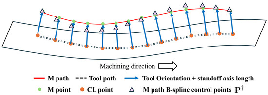
Figure 3.
Schematic diagram of the introduced M path represented by a B-spline curve and its control points to be optimized.
Similar to (19), the integrated jerk along the entire M path is minimized through a quadratic objective function. It is expressed in terms of as
where the Hessian matrix is the same used in (18), as the B-spline knot vector is unchanged.
The geometric constraint of the optimization problem mandates that the B-spline curve passes through the M points at interpolated arc-length parameters ; the set of can be defined using the B-spline in matrix form with the basis function coefficient matrix as
where is an matrix, in which each row corresponds to a single M point .
As depends on the unknown standoff axis length at , the optimization problem becomes nonlinear and cannot be directly solved. Thus, by integrating (47) into (49) and reorganizing the terms, can be expressed as a linear function of as
where is an column vector, while and are expressed using the pseudo inverse of B-spline coefficient matrix as
Then, according to (49)–(52), the objective function in (48) can be expanded in quadratic form in terms of as
where is a positive definite symmetric matrix and is a column vector. The detailed mathematic derivation is reported in Appendix A.
The optimization problem in QP form has to incorporate the objective function (53) with the inequality kinematic constraints to limit the length of the standoff axis within the stroke as
The geometric constraints will be detailed in the next section.
2.4. GFD Construction in 3D Space and Iterative Processing of RTOs
The C-space method [4,5,11] can be employed for collision-free trajectory planning, providing a robust framework for exploring all possible configurations and ensuring collision avoidance, as demonstrated in our previous work [28]. However, building graphs that define feasible and forbidden zones for each node of the overall trajectory is computationally intensive, particularly when combined with shortest-path optimization. Furthermore, our method incorporates a secondary collision-avoidance process to refine trajectory planning while optimizing the redundant standoff axis.
To create a unique GFD that represents the forbidden areas for the three wrist joints , we extend the rotational axes’ C-space to a three-dimensional representation. Similar research [31] introduced cutter lift height to construct a 3D C-space using inclination and yaw planes. However, the extended GFD in our method incorporates an additional degree of freedom provided by , alongside the rotational axes and , to enhance flexibility. This design is derived from the constrained leading and tilt angles , as illustrated in Figure 4. The detailed process of constructing the GFD from the LCS to the WCS is described in our previous work [28].
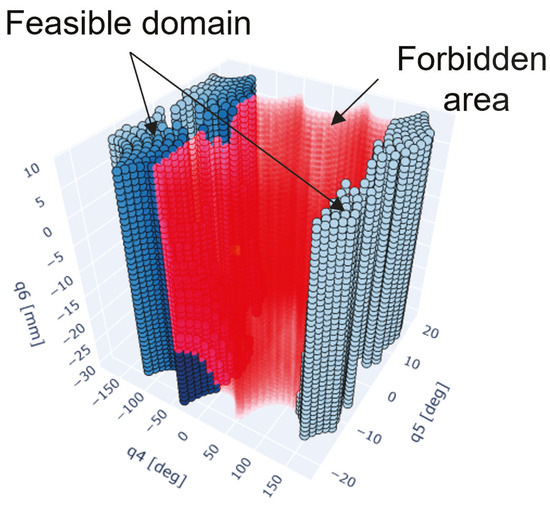
Figure 4.
Proposed 3D GFD on a single CL point. The forbidden areas are indicated within the red regions, and the feasible candidates are represented by the shades of blue corresponding to the distance from the reference point.
It is worth mentioning that the IKT in (3) allows two configurations of the rotational axes for a single tool orientation. However, typical 3D laser head configurations, as shown in Figure 5, result in interference patterns distinct from those of CNC machine tool spindles. Consequently, the proposed GFD is constructed based on wrist joint coordinates, similar to the DAO representation in [7], rather than the tilt and yaw planes used in other studies [5,13].
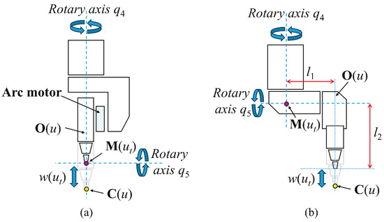
Figure 5.
Mechanical structure of 3D laser cutting heads. (a) Zero-offset head on EFORT machine; (b) conventional head on traditional 3D laser cutting machines with offsets and .
The concept of C-distance, introduced in [5], quantifies the distance between the collided tool orientation and the reference orientation using and angles. The shortest C-distance identifies the minimal change in tool orientation between consecutive local optimal candidates. In our method, the distance equation adopts this principle for consistency. However, since joint trajectories are directly influenced by kinematic constraints, the Euclidean distance is weighted based on the dynamic performance of each joint, as
Here, p represents the index of the non-collided candidate within the feasible region of the ith GFD. The value serves as the reference joint configuration derived via IKT based on the geometric features of RTOs at the ith CL point among initialized or updated RTO collections. Additionally, , , and serve as the dynamic weights in this process.
The RTO-based processing strategy, initially introduced in [3], minimizes collisions and mitigates abrupt tool orientation changes by leveraging RTOs. This strategy involves three main steps to generate a collision-free trajectory:
- Initialize RTOs: Define initial RTOs to act as via points, serving as the foundation for each joint trajectory.
- Trajectory Optimization: Utilize an optimization algorithm to compute smooth, feasible trajectories, leveraging the current set of RTOs as constraints.
- Update RTOs: Add new RTOs when necessary and iteratively refine the optimization process until the entire trajectory is verified to be collision-free.
This iterative method systematically refines the trajectory, eliminating collisions and preserving smooth tool orientations along the entire path. The initial selection of RTOs is crucial for successful trajectory optimization. It significantly impacts both the convergence speed of the optimization algorithm and the effectiveness of collision avoidance. A well-chosen set of RTOs enables the efficient exploration of feasible domains, facilitating the identification of smooth, collision-free trajectories. Conversely, an inadequate or poorly initialized selection of RTOs can lead to suboptimal trajectory solutions, increased computational time or even failure to find a collision-free path.
The selection of initial RTOs should prioritize candidates with minimal Euclidean distance to identify the closest safe ones between the candidate and the ith GFD. Additionally, the relative distance between two adjacent RTOs concerning the segment length should be considered to avoid abrupt changes in tool orientation. A greedy algorithm (i.e., Dijkastra algorithm) addresses this problem by optimizing a multi-objective function. This function, parameterized by the decision variable , represents all the defined RTOs and is expressed as
where indicates the Euclidean distance between two adjacent RTOs, and represents the tool path length between the CL points and . Here, and are the weights assigned to the two components of the objective function to be tuned.
Let be the arc length parameter corresponding to the resolved RTO for . The spline form of a set of joint coordinates can be represented as follows
According to (27), (36) and (43), the above set of via joint coordinates can be expressed as an equality constraint equation in the following form:
where is the coefficient matrix and is the vector including , as follows
At least two RTOs are required, typically specified at the start and the end of the tool path. Once a collision occurs with the currently generated trajectory, the dynamic dimension of the equality constraint matrix needs to be updated by inserting new RTOs into the optimization equations during iterative processing.
The final formulation of the minimized jerk trajectory optimization for the rotational axes, incorporating the additional geometric equality constraint (58), can be expressed as an extension of (43):
Similarly, the geometric equality constraint for the extension value of the redundant standoff axis must be incorporated into (54). The design variable must be constrained within the feasible domain to ensure collision-free conditions during the adjustment of . Consequently, the minimized jerk optimization problem for the M path can be refined as follows:
where is an coefficient matrix with a single value of ‘1’ in the column corresponding to as a row vector , and zeros elsewhere. The vector is , containing the values of . These matrices are defined as follows:
2.5. Summary of the Methodology
The proposed MJTO algorithm for 3D laser cutting machines integrates smoothness optimization, collision avoidance, and redundancy exploitation. Figure 6 illustrates the structured, iterative process of the methodology:
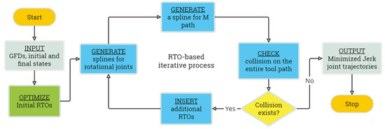
Figure 6.
Flow chart of MJTO algorithm.
Initial RTO Optimization: Initial RTOs are refined to minimize orientation changes and align with reference points according to (56), forming the basis for trajectory planning.
Rotational Joint Trajectory Generation: B-spline modeling (5) is used to generate minimized jerk for the displacement of rotational axis trajectories according to the QP optimization (61), ensuring smooth motion satisfying the kinematic constraints (15) and the geometric constraints (58) in the GFDs.
M Path Optimization: The redundant standoff axis trajectory, modeled with B-splines as (47), is optimized via a separate QP problem in (62) to achieve collision-free via points and smooth translational motion.
Collision Checking: The entire tool path is checked for collisions. Detected collisions are resolved by introducing additional RTOs as constraints with the shortest distance in (55), repeating the trajectory generation.
Iterative Refinement: The process cycles through rotational axes generation, M path optimization, and collision checking until achieving a smooth, collision-free trajectory.
As shown in Figure 6, this methodology ensures collision-free operation while balancing smoothness and precision. By integrating B-spline-based MJTO, iterative refinement, and redundancy exploitation, the framework excels in high-speed, high-precision machining.
3. Illustrative Simulations on B-Pillar Machining
The proposed Minimized Jerk Trajectory Optimization method was implemented in Python 3.11.8 using CVXPY for QP modeling and interfaced with the MOSEK 10.2.5 solver [32]. While the QP-based structure facilitates efficient optimization, the computational costs are affected by the complexity of 3D geometric representations for collision detection and the iterative nature of the RTO-based framework. At this stage, the proposed algorithm runs in an offline computation on a PC platform with a i5-10210U CPU (1.6 GHz, 8-core) and 32 GB of RAM. Two typical cases are presented to demonstrate the effectiveness and advancements of the method, illustrated with an automotive component, as shown in Figure 7. The first case study illustrates the methodology in a straightforward and long machining scenario with minimal tool orientation variation, whereas the second case compares the proposed algorithm with our previous work [28] in a challenging corner scenario involving significant tool orientation adjustments.
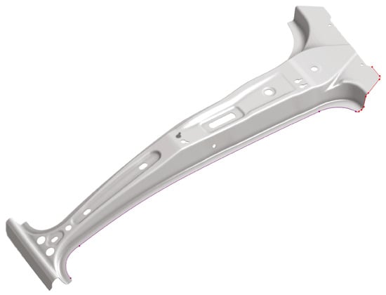
Figure 7.
B-pillar workpiece and corresponding tool paths. The purple line shows the trajectory followed in Case 1, while the red line shows that of Case 2.
The data of machining parameters and joint kinematics parameters used in the following two cases are provided in Table 1 and Table 2.

Table 1.
Machining parameters.

Table 2.
Joint kinematic parameter of the objective laser machine.
3.1. Case Study 1: Long Segment Machining
This study case aims to illustrate the application of the proposed minimized jerk trajectory optimization method in a straightforward machining scenario. The trajectory details and corresponding 3D GFDs across six RTOs for a long segment with minor tool orientation variations are depicted in Figure 8.
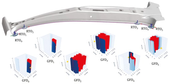
Figure 8.
The long tool path in purple line and its corresponding RTOs, represented as six GFDs for Case 1 prior to optimization.
This scenario involves simulating the machining of a long, straight segment on the side of the B-pillar workpiece using the Python-based physical simulation environment pybullet, as shown in Figure 9. The initial path of the tool, generated without optimization, is shown in Figure 9a. However, Figure 9b illustrates an accidental collision between the cutting head and the workpiece caused by significant adjustments in joint angle following the conventional QI interpolation result, despite the minor angle variations between the initial RTOs.
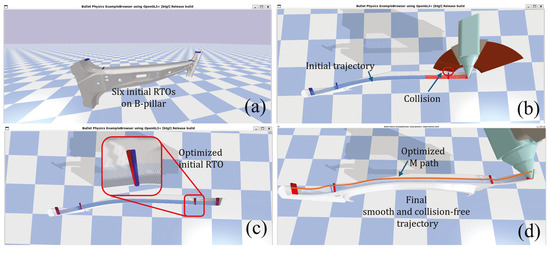
Figure 9.
Pybullet simulation of the long trajectory using the MJTO algorithm for case study 1. (a) Initial position setup and six RTOs shown in blue; (b) collision observed with the original trajectory using QI interpolation, highlighted in red; (c) zoomed-in view of the initial RTO adjustments, optimized via Equation (56) transitioning from the blue RTO to the updated red RTO; (d) final trajectory with the optimized M path represented by the orange line.
The optimal trajectory is obtained within the first iteration of the optimization process, as shown in Figure 9d. Consequently, no additional RTOs are needed, as no further collisions are detected due to the effective initial RTO optimization depicted in Figure 9c. After optimizing the initial RTOs to ensure a collision-free trajectory, the angular changes between consecutive RTOs were carefully controlled. By keeping these angle adjustments within the tolerance for the allowable processing error, excessive movements in the joint were avoided, even with minimal changes in tool orientation.
The joint trajectory plots in Figure 10 highlight the significantly smoother kinematic performance of the proposed MJTO algorithm compared to the conventional QI method. This smoothness is evident across velocity, acceleration, and jerk levels, primarily due to the global optimization applied across all RTOs. Unlike the traditional QI method, which often causes discontinuities in acceleration and jerk between trajectory segments, the MJTO algorithm ensures holistic trajectory optimization, minimizing abrupt motion changes. This improvement not only enhances machining precision, but also reduces mechanical stress and wear on cutting components, thereby improving the the longevity and reliability of the manufacturing system.
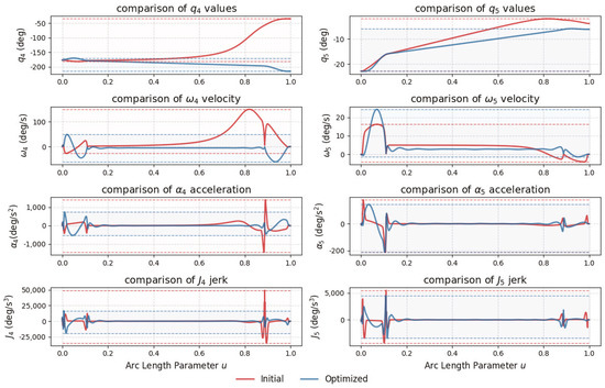
Figure 10.
Comparison of initial (red) and optimized (blue) rotational axes trajectories for position , velocity , acceleration , and jerk levels, along with their boundaries, represented by the dotted lines.
Furthermore, with the assistance of the high dynamic performance of the redundant standoff axis, the curvature of the M trajectory was optimized, resulting in improved performance on the translational axes. Although the original tool path in this case is relatively simple and long, posing minimal challenges to most translational axes, the integration of the redundant axis allows for finer control and smoother motion even in straightforward scenarios. This ensures translational movements are not only smoother, but also more efficient, contributing to reduced mechanical stress and improved overall system performance. The benefits of the redundant standoff axis become more evident in complex tasks, such as sharp corner navigation, as it will be demonstrated in the following case study, which validates the effectiveness of the MJTO algorithm in enhancing trajectory smoothness and reducing mechanical stress.
3.2. Case Study 2: Shape Corner Segment Machining
Sheet metal components with large angles of bend are exceedingly common in the automotive manufacturing industry. These pronounced bends pose significant challenges for 3D LCM processes. To meet high-speed machining requirements, the tool orientation must execute rapid and substantial rotations within short segments to accurately cut the lateral surfaces of bent sheet metal. In this case, the objective trajectory follows an irregular and complex corner surface with ten RTOs at key waypoints, as illustrated in Figure 11. Notably, there are two significant orientation changes of approximately between adjacent tool orientations over short distances, posing a major challenge for smooth trajectory planning. This scenario, also considered in our previous work [28], demonstrates the effectiveness of the proposed optimization method in handling large-angle rotations smoothly and maintaining collision-free machining under demanding conditions. Furthermore, the optimized M trajectory, based on the proposed redundant standoff axis, ensures smoother translational motions during high-curvature machining, further enhancing overall performance and reliability.
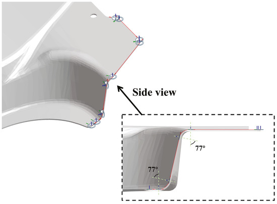
Figure 11.
The objective trajectory on the target surface with a side view; note the angular deviation between two adjacent tool orientations.
The experimental test data can be summarized as follows. The initial tool-path trajectory is interpolated by a standard G-code interpolator using QI for the orientation, leading to a total machining time of 2.51 s with the dynamic machining parameters. Based on the 4 ms sampling interval ( = 4 ms) of the motion controller, 628 CL points are generated. The proposed MJTO framework demonstrates significant computational advantages compared to our previous graph-based method: While conventional collision checking required exhaustive evaluation at all 628 CL points, our current implementation significantly reduces the number of collision detection operations from 628 to 12 critical RTO positions. Calculating the large-scale Hessian matrix in (18) takes 9.5 s, while the QP solver in CVXPY requires an additional 0.8s of computation time, yielding a total optimization time faster than the time of our prior approach. This acceleration stems from both reduced collision detection iterations and the unified 3D GFD method introduced in Section 2.4, which eliminates three axes collision checks together.
Figure 12 illustrates the evolution of RTOs throughout the optimization stages. In Figure 12a, the initial RTOs are first reselected to minimize abrupt angle changes in the short segments. This redistributes angular adjustments across multiple RTOs (Figure 12b). In subsequent iterations (Figure 12c), additional RTOs are inserted when intermediate collisions or interference issues are detected. These extra RTOs serve as additional constraints in the optimization. Ultimately, the minimized-jerk planning produces a smoother, collision-free trajectory, as shown in Figure 12d.
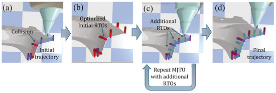
Figure 12.
Evolution of RTOs through the optimization process: (a) initial RTOs; (b) RTOs after the first optimization; (c) additional RTOs added; (d) final collision-free and smoother trajectory.
To demonstrate the improvement in smoothness, Figure 13 compares the rotational axes and among three methods: the initial trajectory generated by quaternion interpolation (blue), a graph-based approach (green), and the proposed MJTO algorithm (orange). In the position plots, MJTO noticeably alters the original profile, redistributing the large angular changes more evenly. This is enabled by adjusting the RTOs in the early phases. In terms of acceleration, MJTO achieves much smaller and fewer spikes than the other two methods, indicating reduced dynamic stress and smoother motion when facing large orientation changes. However, one should note that the B-spline curves used here may produce overshooting or oscillations between non-keyway points in the trajectory, as they minimize the integral of the jerk over the entire path. This phenomenon can introduce angular errors or posture drifts, especially in regions of high curvature.
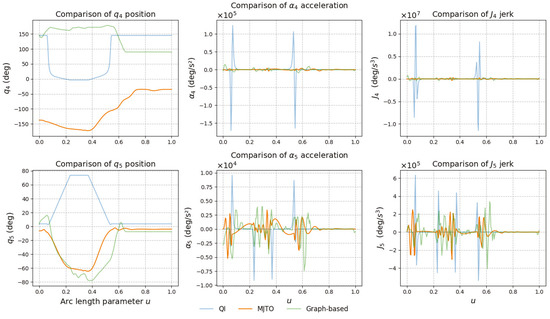
Figure 13.
Comparison of rotational axes and in position (left), acceleration (center), and jerk (right) among QI (blue), graph-based (green), and MJTO (orange) methods.
Beyond the rotational axes, we also optimized the redundant translational axis M. Figure 14 compares the M path trajectory generated by QI (yellow) and MJTO (red) from the CL tool path (blue). By eliminating unnatural “knot” bends, the MJTO-based approach achieves a much smoother, more continuous path, which is particularly advantageous for high-speed machining tasks, where excessive velocity or acceleration discontinuities can lead to vibrations or inaccuracy.
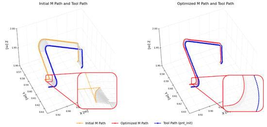
Figure 14.
Comparison of M paths before (QI in blue) and after (MJTO in orange) optimization. A zoomed view highlights how MJTO smooths out any abrupt “knot” in the original path.
A more detailed view of smoothness enhancement can be observed in Figure 15, where are compared in terms of position, acceleration, and jerk. The MJTO trajectories (orange) show significantly reduced acceleration peaks and smoother jerk profiles compared to QI (blue) and graph-based methods (green). To better visualize the distribution of jerk values for each joint, Figure 16 shows a violin plot, where the horizontal axis represents different planning methods QI, graph-based, and MJTO, whereas the vertical axis shows the corresponding range and probability distribution of jerk for each joint. The “width” of the violin at each vertical level indicates how densely the jerk values are concentrated around that magnitude. Therefore, narrower violins (especially at higher jerk magnitudes) indicate fewer extreme jerk values; from these plots, one can see that MJTO’s distributions tend to be narrower and more centered around lower jerk levels, implying a significant improvement in smoothness.
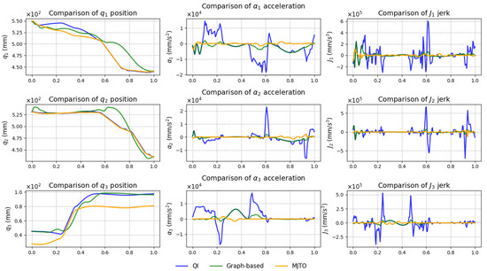
Figure 15.
Translational joints under QI, graph-based, and MJTO: position (left), acceleration (center), and jerk (right).

Figure 16.
Violin plots of jerk distributions across five main axes ( to ) for QI, graph-based, and MJTO methods. The horizontal axis indicates different methods; the vertical axis is the jerk value. Narrower shapes at high jerk ranges signify fewer extreme jerk points, reflecting smoother overall motions.
In summary, by introducing refined RTO placement and employing minimized-jerk B-spline planning, the proposed MJTO method effectively handles large-angle rotations (up to ) while also enhancing the smoothness of both the rotational and translational axes. Compared to the QI and graph-based methods, MJTO demonstrates smaller acceleration peaks, reduced jerk, and fewer sudden orientation shifts. Although local overshoots may arise from the spline formulation, these can be controlled through additional keyway constraints until machining precision and posture accuracy are satisfied. Overall, the MJTO approach provides a stable, high-speed solution for sheet-metal corner-segment machining, ensuring accuracy and collision-free performance even under significant orientation variations.
4. Conclusions and Future Work
In this study, we presented a novel trajectory optimization strategy specifically for 3D laser cutting machines equipped with a redundant standoff axis. Building on our previous work, the proposed approach employs a Minimized Jerk Trajectory Optimization framework with B-spline modeling to formulate two QP tasks: one focus on smoothing the rotational axes trajectories and the other dedicated to refining the M path governed by the redundant standoff axis. By integrating an iterative RTO-based optimization process within the feasible domains defined by the 3D joint-coordinate GFD, our method not only reduces abrupt angular transitions among multiple RTOs, but also significantly improves the continuity of the translational axis movements. Consequently, the optimized trajectories demonstrated enhanced smoothness, reduced mechanical stress, and consistent collision-free operation.
The effectiveness of our proposed method was demonstrated through two simulation cases involving the machining of an automotive B-pillar workpiece. In the first case, characterized by minimal orientation changes, a single iteration of our algorithm successfully produced a smooth, collision-free trajectory. Kinematic performance evaluations revealed reductions in acceleration and jerk peaks compared to the conventional QI method, underscoring the improved trajectory stability. In the second more demanding case featuring large-angle rotations and high-curvature corners, our iterative strategy effectively managed abrupt orientation transitions by strategically inserting additional RTOs and leveraging optimized adjustment to the M path. These results highlight the method’s capability of accommodating complex geometries while maintaining trajectory smoothness and ensuring precise, collision-free movements.
Future work will explore the expension of the optimization framework to more intricate machining scenarios and broader industrial applications. While a constant feedrate assumption was adopted in this study, future research could incorporate adaptive feedrate control strategies to further enhance the trajectory smoothness. Additionally, integrating real-time collision detection and avoidance mechanisms will be investigated to accommodate unexpected disturbances. Meanwhile, two specific open issues remain to be addressed. First, since the free-form nature of B-splines can occasionally introduce local overshoot or oscillations, employing monotonic spline interpolation strategies [33] may help to mitigate these effects by enforcing strictly monotonic interpolation patterns. Second, further algorithmic refinements of MJTO, along with more computationally efficient implementations for the RTO insertion process, could reduce the computational overhead and improve scalability. Lastly, future efforts will include experimental validations conducted on physical laser cutting machines to verify simulation results and assess practical machining performance.
Author Contributions
Writing—original draft preparation, Z.D.; writing—review and editing, M.I. and A.R.; supervision, M.I. and A.R. All authors have read and agreed to the published version of the manuscript.
Funding
This research received no external funding.
Data Availability Statement
Data are contained within the article.
Acknowledgments
The authors gratefully acknowledge EFORT Europe s.r.l. for sponsoring the Industrial Ph.D. project. Author Z.D. would like to extend his sincere appreciation to his colleagues Pietro Soccio and Daniele Costamagna for their invaluable inspiration and insightful contributions during the technical discussions.
Conflicts of Interest
Author Zhipeng Ding is employed by the company EFORT Europe s.r.l. The authors declare that the research was conducted in the absence of any commercial or financial relationships that could be construed as a potential conflict of interest.
Abbreviations
The following abbreviations are used in this manuscript:
| LCM | laser cutting manufacturing |
| CNC | computer numerical control |
| CL | cutter location |
| WCS | workpiece coordinate system |
| MCS | machine coordinate system |
| LCS | local coordinate system |
| IKT | inverse kinematic transformation |
| C-space | Configuration space |
| DAO | domain of admissible orientation |
| GFD | geometric feasible domain |
| RTO | representative tool orientation |
| QP | quadratic programming |
| QI | quaternion interpolation |
| MJTO | minimized jerk trajectory optimization |
Appendix A. Derivation of the Quadratic Objective Function
In this appendix, we provide a concise derivation of the quadratic objective function used to minimize the integrated jerk along the M path.
Starting from the relationship between the control points and the redundant standoff axis defined in (50), the objective function defined in (48) can be rewritten as
Expanding the quadratic form as
the objective function can be finally expressed in the standard quadratic form
where the components are defined as
As the constant part c of the quadratic objective function can be omitted, this formulation transforms the optimization problem into a standard QP form in (53), facilitating an efficient solution using QP solvers.
References
- Alsaadawy, M.; Dewidar, M.; Said, A.; Maher, I.; Shehabeldeen, T.A. A comprehensive review of studying the influence of laser cutting parameters on surface and kerf quality of metals. Int. J. Adv. Manuf. Technol. 2024, 130, 1039–1074. [Google Scholar] [CrossRef]
- Beudaert, X.; Pechard, P.Y.; Tournier, C. 5-Axis tool path smoothing based on drive constraints. Int. J. Mach. Tools Manuf. 2011, 51, 958–965. [Google Scholar] [CrossRef]
- Ho, M.C.; Hwang, Y.R.; Hu, C.H. Five-axis tool orientation smoothing using quaternion interpolation algorithm. Int. J. Mach. Tools Manuf. 2003, 43, 1259–1267. [Google Scholar] [CrossRef]
- Lauwers, B.; Dejonghe, P.; Kruth, J. Optimal and collision free tool posture in five-axis machining through the tight integration of tool path generation and machine simulation. Comput.-Aided Des. 2003, 35, 421–432. [Google Scholar] [CrossRef]
- Jun, C.S.; Cha, K.; Lee, Y.S. Optimizing tool orientations for 5-axis machining by configuration-space search method. Comput.-Aided Des. 2003, 35, 549–566. [Google Scholar] [CrossRef]
- Tutunea-Fatan, O.R.; Feng, H.Y. Configuration analysis of five-axis machine tools using a generic kinematic model. Int. J. Mach. Tools Manuf. 2004, 44, 1235–1243. [Google Scholar] [CrossRef]
- Castagnetti, C.; Duc, E.; Ray, P. The domain of admissible orientation concept: A new method for five-axis tool path optimisation. Comput.-Aided Des. 2008, 40, 938–950. [Google Scholar] [CrossRef]
- Wang, N.; Tang, K. Five-axis tool path generation for a flat-end tool based on iso-conic partitioning. Comput.-Aided Des. 2008, 40, 1067–1079. [Google Scholar] [CrossRef]
- Wang, Y.; Xu, J.; Sun, Y. Tool orientation adjustment for improving the kinematics performance of 5-axis ball-end machining via CPM method. Robot. Comput.-Integr. Manuf. 2021, 68, 102070. [Google Scholar] [CrossRef]
- Plakhotnik, D.; Lauwers, B. Graph-based optimization of five-axis machine tool movements by varying tool orientation. Int. J. Adv. Manuf. Technol. 2014, 74, 307–318. [Google Scholar] [CrossRef]
- Mi, Z.; Yuan, C.M.; Ma, X.; Shen, L.Y. Tool orientation optimization for 5-axis machining with C-space method. Int. J. Adv. Manuf. Technol. 2017, 88, 1243–1255. [Google Scholar] [CrossRef]
- Xu, H.; Hu, J.; Wu, W. Optimization of 3D laser cutting head orientation based on the minimum energy consumption. Int. J. Adv. Manuf. Technol. 2014, 74, 1283–1291. [Google Scholar] [CrossRef]
- Xu, J.; Zhang, D.; Sun, Y. Kinematics performance oriented smoothing method to plan tool orientations for 5-axis ball-end CNC machining. Int. J. Mech. Sci. 2019, 157, 293–303. [Google Scholar] [CrossRef]
- Xiao, Q.B.; Wan, M.; Zhang, W.H.; Yang, Y. Tool orientation optimization for the five-axis CNC machining to constrain the contour errors without interference. J. Manuf. Process. 2022, 76, 46–56. [Google Scholar] [CrossRef]
- Wu, L.; Xu, J.; Yin, X.; Sun, Y. Jerk-optimal piecewise planning of tool orientation for 5-axis ball-end machining with linearized kinematic constraints. J. Manuf. Sci. Eng. 2023, 145, 071003. [Google Scholar] [CrossRef]
- Huang, K.T.; Zhang, Z.; Gong, H.; Li, Z.; Fang, F.; Wang, D. Constructing smooth tool orientation field based on radial basis function for 5-axis machining. Int. J. Adv. Manuf. Technol. 2017, 91, 1369–1379. [Google Scholar] [CrossRef]
- Langeron, J.M.; Duc, E.; Lartigue, C.; Bourdet, P. A new format for 5-axis tool path computation, using Bspline curves. Comput.-Aided Des. 2004, 36, 1219–1229. [Google Scholar] [CrossRef]
- Yuen, A.; Zhang, K.; Altintas, Y. Smooth trajectory generation for five-axis machine tools. Int. J. Mach. Tools Manuf. 2013, 71, 11–19. [Google Scholar] [CrossRef]
- Li, D.; Zhang, W.; Zhou, W.; Shang, T.; Fleischer, J. Dual NURBS path smoothing for 5-axis linear path of flank milling. Int. J. Precis. Eng. Manuf. 2018, 19, 1811–1820. [Google Scholar] [CrossRef]
- Sharon, A.; Hogan, N.; Hardt, D.E. The macro/micro manipulator: An improved architecture for robot control. Robot. Comput.-Integr. Manuf. 1993, 10, 209–222. [Google Scholar] [CrossRef]
- Quan, B.T.; Huang, J.; Harada, M.; Yabuta, T. Control of a macro-micro robot system using manipulability of the micro robot. JSME Int. J. Ser. C Mech. Syst. Mach. Elem. Manuf. 2006, 49, 897–904. [Google Scholar] [CrossRef][Green Version]
- Zhou, Y.; Chen, C.Y.; Yang, G.; Li, Y. A sampling-based motion assignment strategy with multi-performance optimization for macro-micro robotic system. IEEE Robot. Autom. Lett. 2022, 7, 11649–11656. [Google Scholar] [CrossRef]
- Kakinuma, Y.; Ogawa, S.; Koto, K. Robot polishing control with an active end effector based on macro-micro mechanism and the extended Preston’s law. Cirp Ann. 2022, 71, 341–344. [Google Scholar] [CrossRef]
- Cursi, F.; Bai, W.; Yeatman, E.M.; Kormushev, P. Optimization of surgical robotic instrument mounting in a macro–micro manipulator setup for improving task execution. IEEE Trans. Robot. 2022, 38, 2858–2874. [Google Scholar] [CrossRef]
- Uzunoglu, E.; Dede, M.I.C.; Kiper, G. Trajectory planning for a planar macro-micro manipulator of a laser-cutting machine. Ind. Robot. Int. J. 2016, 43, 513–523. [Google Scholar] [CrossRef]
- Liu, J.; Xie, X.; Zhou, Z.; Gao, W.; Liang, Z. Research on high-speed and high-precision laser processing algorithm based on macro-micro platform. Proc. Inst. Mech. Eng. Part B J. Eng. Manuf. 2023, 237, 899–910. [Google Scholar] [CrossRef]
- Ding, Z.; Soccio, P.; Indri, M.; Rizzo, A. Through hole-cutting conic posture optimization for a redundant 3D laser cutting machine. Int. J. Adv. Manuf. Technol. 2024, 132, 443–461. [Google Scholar] [CrossRef]
- Ding, Z.; Indri, M.; Rizzo, A.; Soccio, P. Smooth and Collision-Free Trajectory Planning for Redundant 3D Laser Cutting Machines. In Proceedings of the 2024 IEEE 29th International Conference on Emerging Technologies and Factory Automation (ETFA), Padova, Italy, 10–13 September 2024. [Google Scholar]
- Gordon, W.J.; Riesenfeld, R.F. B-spline curves and surfaces. In Computer Aided Geometric Design; Elsevier: Amsterdam, The Netherlands, 1974; pp. 95–126. [Google Scholar]
- Hu, P.; Tang, K. Improving the dynamics of five-axis machining through optimization of workpiece setup and tool orientations. Comput.-Aided Des. 2011, 43, 1693–1706. [Google Scholar] [CrossRef]
- Lu, J.; Cheatham, R.; Jensen, C.; Chen, Y.; Bowman, B. A three-dimensional configuration-space method for 5-axis tessellated surface machining. Int. J. Comput. Integr. Manuf. 2008, 21, 550–568. [Google Scholar] [CrossRef]
- Mosek ApS. The MOSEK Optimization Toolbox for MATLAB Manual, version 10.1; Mosek ApS: Copenhagen, Denmark, 2024. [Google Scholar]
- Fritsch, F.N.; Butland, J. A method for constructing local monotone piecewise cubic interpolants. SIAM J. Sci. Stat. Comput. 1984, 5, 300–304. [Google Scholar] [CrossRef]
Disclaimer/Publisher’s Note: The statements, opinions and data contained in all publications are solely those of the individual author(s) and contributor(s) and not of MDPI and/or the editor(s). MDPI and/or the editor(s) disclaim responsibility for any injury to people or property resulting from any ideas, methods, instructions or products referred to in the content. |
© 2025 by the authors. Licensee MDPI, Basel, Switzerland. This article is an open access article distributed under the terms and conditions of the Creative Commons Attribution (CC BY) license (https://creativecommons.org/licenses/by/4.0/).