Abstract
Aerostatic conical bearings with micro-orifices (ACBMOs) can simultaneously withstand both radial and axial external loads and have high power density. Nevertheless, due to the larger surface-to-volume ratio and length-to-diameter ratio of micro-orifices, the gas flow through micro-orifices is more susceptible to frictional loss. Since frictional loss in micro-orifices has been ignored in the literature, an aerostatic conical bearing lubrication model with frictional loss in micro-orifices and a transient model of their nonlinear dynamics are established. The effects of the micro-orifice length-to-diameter ratio and relative roughness on lubrication performance, nonlinear behaviors, and ACBMO–rotor system stability are investigated, followed by experimental validation. The results indicate that the gas mass flow rate of the micro-orifices, gas film pressure, and load capacity in the ACBMOs decrease with the increase in micro-orifice relative roughness and length-to-diameter ratio, which cannot be observed in the conventional model without frictional loss. Meanwhile, both the onset speed of instability and the failure speed decrease when frictional loss occurs in micro-orifices are considered.
1. Introduction
Aerostatic conical bearings exhibit low viscous dissipation and generate minimal temperature increases during high-speed rotation. Meanwhile, they can simultaneously withstand both radial and axial external loads, which is conducive to minimizing the volume of the equipment and increasing their power density, thus holding broad application prospects in the field of ultra-precision machining [1,2]. However, they cannot meet the requirements of high load capacity and high stiffness in ultra-high-speed motorized spindle equipment because of the compressibility and low viscosity of gas lubrication. Although recesses with various shapes have been manufactured at the exits of aerostatic bearings’ inherent orifices to enhance the load capacity of ACBMOs, the airflow more easily generates vortices at the recesses, eventually culminating in micro-vibrations [3]. Recently, studies have demonstrated that the performance of aerostatic bearings can be improved with micro-orifice diameters below 0.1 mm [4,5], and the pressure distribution can be made more even in the bearing clearance by reducing the diameters of the micro-orifices [6,7,8].
However, due to limitations in micro-orifice machining, the flow in the micro-orifices of aerostatic conical bearings will be influenced by frictional loss from the relative roughness of the micro-orifices’ walls. Meanwhile, the flow through micro-orifices can be described on a micro scale for fluid flow in microchannels due to the large surface-to-volume and length-to-diameter ratios of micro-orifices. Mohiuddin Mala et al. [9] conducted experiments on microchannels with diameters of 50–254 μm and a relative roughness of 0.69–3.5%. The results indicated that the mass flow in microchannels can be affected by wall roughness when the diameter of the microchannels decreases and the Reynolds number increases. A systematic investigation of flow characteristics through microchannels with diameters varying from 44.5 to 1011 μm was conducted by Chen et al. [10], and the results showed that when the friction factor increases, early transition occurs, and the critical Reynolds number decreases as the diameter of the microchannels decreases. The modified roughness viscosity model was employed to numerically simulate the flow characteristics of compressible gas, which demonstrated that wall roughness causes early transition and mass flow loss [11]. For microchannel gas flows with a relative roughness < 1%, the experimental friction factors in Tang et al.’s study [12] validate the theoretical model f = 0.3164 Re−1/4, but the friction factors predicted through the theoretical model deviate from experimental findings for relative roughness values exceeding 1%. Li et al. [13] demonstrated that the fluid flow rate at the microchannel outlet decreases as the surface roughness increases through a random rough surface model solved by COMSOL, and they found that vortices are formed in the rough surface of these microchannels. Overall, the relative roughness of micro-orifices impacts the flow rate when it exceeds 1%. Unfortunately, no research has been reported studying a lubrication model of ACBMOs that considers the frictional loss in micro-orifices.
On the other hand, due to the compressibility and low-damping characteristics of gas lubrication, the ACBMO–rotor system becomes more unstable at higher rotational speeds. Additionally, in nonlinear dynamic analysis, the critical rotational speed can be categorized into the onset speed of instability and the failure speed. The onset speed of instability is characterized by the initial emergence of sub-synchronous vibration [14]. When the rotational speed exceeds the onset speed of instability, it leads to contact failure between the rotor and bearing. The speed is referred to as the failure speed when rotor–bearing contact occurs [15]. The nonlinear behaviors and stability of aerostatic bearing–rotor systems are related to the lubrication model. A bidirectional fluid–structure coupling dynamic model of this system was established in [16]. The results showed that the trend of the recess flow changes similarly to the rotor vibration, and the system exhibits pneumatic hammer instability as rotational speed increases. Chen et al. [17] conducted a comprehensive study by incorporating manufacturing errors in bearing sleeves into an aerostatic bearing lubrication model. As a result, the manufacturing errors disrupted the symmetry of the gas film, inducing pressure oscillations periodically with time, while convexity errors weakened the system stability. An ACB–rotor system with 0.03 mm diameter micro-orifices was investigated by Zheng et al.; however, their analysis did not account for the influence of micro-orifice frictional loss on the orifice flow [18]. Thus, throughout the above literature, the frictional loss in micro-orifices has been ignored in the current aerostatic bearing–rotor system model.
In this study, an ACBMO model incorporating frictional loss in micro-orifices, along with a nonlinear transient model, is established and experimentally validated. Next, the effects of the micro-orifice length-to-diameter ratio and relative roughness on the mass flow rate and lubrication performance of the ACBMO are investigated. Furthermore, the effects of micro-orifice frictional loss on the nonlinear behaviors of an ACBMO–rotor system are examined. We seek to establish a foundation for evaluating the stability of high-speed ACBMO–rotor systems and designing ACBMOs.
2. Mathematical Model of Bearing–Rotor System with Frictional Loss
2.1. The Governing Equation of Air Film Flow
Figure 1a illustrates the structure of ACBMOs, including two rows of micro-orifices. The schematic of the rotor in ACBMOs and the relationship between the conical and Cartesian coordinate systems are shown in Figure 1b and Figure 1c, respectively. The relationship between the bearing radius R and the axial coordinate r is derived as follows [18]:
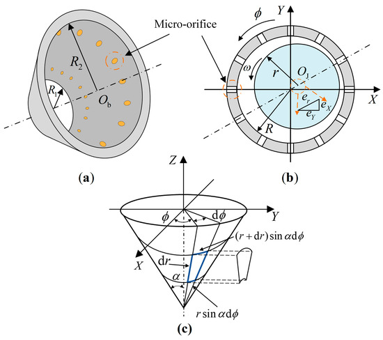
Figure 1.
(a) Structure of ACBMOs; (b) schematic of the rotor in an aerostatic conical bearing; (c) the conical coordinate system.
Integration of the fundamental governing equations (continuity, momentum, and the ideal gas state equation) yields the transient isothermal compressible Reynolds equation in conical coordinates, which describes the lubrication characteristics of ACBMOs:
where ϕ denotes the circumferential coordinate; r represents the axial coordinate; p represents the pressure of the air film; h represents the air film thickness. The normalized values are defined as follows: , and the Kronecker function is given by
The parameters after the conformal transformation are derived:
The gas mass flow coefficient is defined as , where the mass flow rate needs to be corrected by , and Cd represents the effect of the bearing clearance on the mass flow through the micro-orifices [19].
The dimensionless form of the Reynolds equation for ACBMOs is obtained as follows:
In the Reynolds equation, the normalized air film thickness is calculated as follows:
where ε and ε* denote the eccentricity ratios for the left bearing ACBMOs (L) and the right bearing ACBMOs (R), respectively. The subscripts indicate the directions corresponding to the eccentricity ratios along the coordinate axes. The dimensionless eccentricity ratios are given by , , and .
Implementation of Equation (6) requires boundary conditions, as illustrated in Figure 2 and specified below:
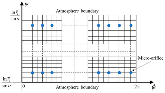
Figure 2.
Computational domain and boundary conditions.
The solution to Equation (6) is obtained by the finite difference method in combination with the under-relaxed Gauss–Seidel iterative method. The bearing load capacities FhX, FhY, and FhZ are then obtained as follows:
The Z-axis load capacity FhZ is taken as positive for the left bearing and negative for the right bearing.
2.2. Micro-Orifice Model with Frictional Loss in Aerostatic Conical Bearings
As illustrated in Figure 3, a model for the gas mass flow rate with frictional loss in micro-orifices is developed. In this model, ps denotes the supply pressure, pin the inlet pressure of the micro-orifices, pori the downstream pressure, dori the diameter of the micro-orifices, and lori the length of the micro-orifices.
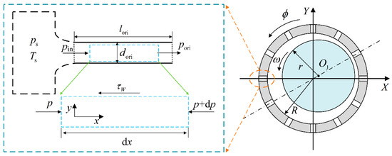
Figure 3.
Micro-orifice model in an aerostatic conical bearing.
The momentum equation for gas flow in constant-area adiabatic frictional micro-orifices is derived as follows:
where f denotes the friction factor, from which the frictional loss is determined according to the Darcy formula [20]:
Equation (10) is combined with and as follows:
Substituting the continuity equation and the energy conservation equation into the ideal gas state equation yields the following governing system:
By combining Equation (12) with Equation (13) and integrating, the relations for the pressure drop with frictional loss are derived as follows:
Solving Equation (14) requires determining the friction factor f for compressible gas flow in micro-orifices. Recent research [21] has shown that f can be obtained by solving the coupled Poisson–Boltzmann and Navier–Stokes equations; however, this approach involves computationally expensive solutions to complex differential equations. To reduce the computational cost, the present study adopts a semi-empirical correlation method. The velocity profile of turbulent flow in the micro-orifice cross-section is shown in Figure 4. Owing to the extreme thinness of the viscous sublayer near the micro-orifice walls, the velocity profile across the entire cross-section can be approximated by the logarithmic distribution characteristic of the turbulent core region, with an equivalent hydraulic wall location at y0.
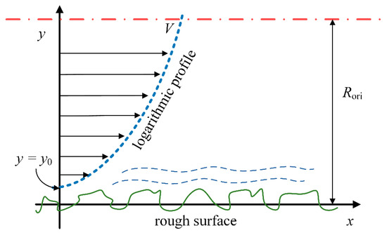
Figure 4.
Turbulent velocity distribution in the cross-section of the micro-orifices.
This relation can be obtained from the combination of the Reynolds stress tensor and Prandtl’s mixing length hypothesis [22]:
where τturb denotes the turbulent shear stress and lmix the characteristic turbulent scale. Subsequently, the equation for the friction factor f in terms of relative roughness and Reynolds number is derived by integrating Equation (15) and combining it with the wall shear stress:
where κ1 denotes the Karmann constant and κ2 denotes the ratio of the viscous sublayer thickness y0 to the radius of the micro-orifices. Both κ1 and κ2 are empirical parameters obtained from Tang’s study on the gas flow characteristics in microchannels [12]. According to Tang’s results, the friction factor f can be calculated using Churchill’s equation [23], with relative errors of less than 5%.
The mass flow rate accounting for frictional loss in micro-orifices can be expressed as
where the Mach number Ma can be calculated using Equation (14).
2.3. Dynamic Model of the ACBMO–Rotor System
The discretization of the conical rotor is illustrated in Figure 5, where Lr denotes the length of the rotor, Rs1 the outer radius, and Rs2 the inner radius. The system matrices are derived based on Timoshenko beam theory, which accounts for shear deformation and gyroscopic effects. Geometrically, the conical sections are represented by equivalent cylindrical models, while certain segments are modeled with hollow cross-sections.
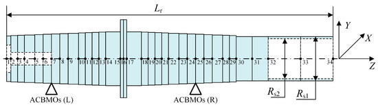
Figure 5.
Schematic of the ACBMO–rotor system.
The displacement vector in different directions is given as follows:
The governing equation for the bending vibrations, based on Timoshenko beam theory [24,25,26], can be expressed as
Assuming a counterclockwise rotor rotation and an unbalance phase angle of 0° for mreu, the resulting unbalance forces QX and QY are given as follows:
The governing equation for axial vibrations is obtained as
By combining Equations (20) and (22), the governing equation of motion for the vibrations of the flexible rotor is derived as follows:
where the mass, stiffness, and gyroscopic system matrices are assembled from element matrices, whose definitions are provided in Appendix A.
2.4. Numerical Calculation
The overall flowchart of this study is illustrated in Figure 6. The left branch presents the lubrication solution algorithm for the parametric analysis of micro-orifices. When the pressure ratio of the micro-orifices falls below the critical ratio βκ, the airflow reaches sonic velocity, where the inlet pressure equals the outlet pressure. Conversely, when the pressure ratio exceeds βκ, the inlet pressure pin must be determined iteratively.
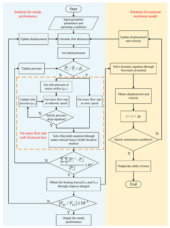
Figure 6.
Flowchart of the ACBMO lubrication model with frictional loss and the transient nonlinear model.
To obtain the nonlinear behaviors of the ACBMO–rotor model with frictional loss, the transient solution of Equation (6) is first obtained using the under-relaxation Gauss–Seidel iterative method. The load capacity is then calculated using the Composite Simpson rule. Finally, the nonlinear behaviors are determined by solving Equation (23). To ensure convergence of the limit cycle, a temporal discretization of 400 steps per period is adopted, and simulation results from the last 200 periods are retained.
2.5. Numerical Model Validation
In the absence of published studies on the coupled transient nonlinear dynamics of the ACBMO–rotor system with frictional loss, the ACBMO lubrication model and the transient nonlinear model are validated independently.
To validate the lubrication model, the results of Fhr are compared with those reported by Zhang et al. [27] by setting the semi-cone angle of the ACBMOs to 0.0001°, as shown in Figure 7a. Additionally, Figure 7b illustrates the orbits of a well-balanced rotor with an aerostatic bearing, obtained by setting the supply pressure to 0.0 MPa [28]. Both sets of computational results exhibit good agreement with the literature, thus confirming the reliability of the numerical model.
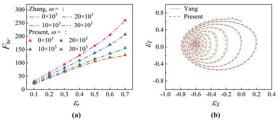
Figure 7.
(a) Comparison of the present simulation of load capacity with Zhang et al. [27]; (b) comparison of the present simulation of orbits with Yang et al. [28].
3. Experiment Validation
To validate the ACBMO–rotor system model with frictional loss, a test rig capable of reaching a maximum rotational speed of 200 krpm has been developed, as shown in Figure 8. The rig consists of three main components: a drive module, a support module, and a vibration testing module. Specifically, the drive module incorporates an air compressor (SMC AMS40 is manufactured by SMC in Tokyo, Japan), an AC frequency converter, and a water-circulation cooling system. A semi-cone angle of 0.0001° is adopted in the model to match the rotor configuration of the test rig (α = 0°). Table 1 lists the parameters of the ACBMOs and rotor employed in the experiments.
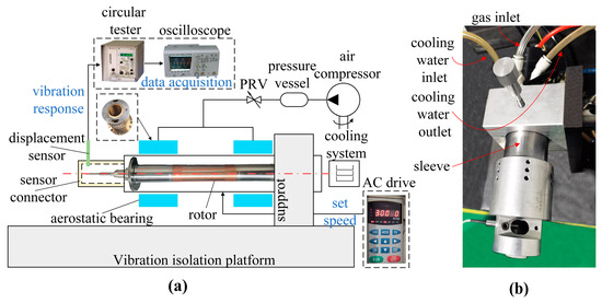
Figure 8.
Rotodynamic test rig: (a) schematic of the experiment rig for aerostatic bearing–rotor vibration analysis; (b) photograph of the aerostatic bearing–rotor system vibration test rig.

Table 1.
The rotodynamic test rig parameters.
As illustrated in Figure 8a, the rotor-end vibration response was first measured using a capacitive displacement sensor with a resolution of 300 nm and a sensitivity of 25 μm/V. Next, analog signals from the circular tester (TARGA Ⅲ is manufactured by Lion Precision in Oakdale, MN, USA) were transmitted in real time to the oscilloscope (DSO5032A is manufactured by Agilent in Beijing, China), which simultaneously displayed the vibration amplitudes. The unbalance at the thrust disk, measured by a dynamic balancing machine, was found to be 0.2118 g·mm. Finally, a reflective marker was attached to extract vibration phase information, although it was not utilized in this study. During marker transit, the displacement sensor recorded a rapid shift in signal amplitude.
Figure 9a presents the denoised and filtered experimental vibration response. The time-domain responses, computed with and without frictional loss in micro-orifices, are compared with the experiment vibration response shown in Figure 9b. Subsequent FFT analysis is performed to extract the frequency-domain characteristics of these three signals, including the experimental signal and two simulated signals. One simulated signal is obtained from the baseline model that neglects the micro-orifice frictional loss [18]. A comparative amplitude analysis shows that the model incorporating frictional loss in micro-orifices results in a 13.3% relative amplitude error with respect to the experimental data, thereby demonstrating improved accuracy over the original model without the frictional loss, as shown in Figure 9c.
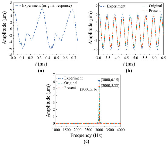
Figure 9.
Experimental results at ω = 180 krpm: (a) experimental response in the time domain; (b) comparative responses in the time domain; (c) comparative amplitude in the frequency domain.
4. Results and Discussion
4.1. Effects of Frictional Loss on Micro-Orifice Performance
In this section, the proposed model for the mass flow rate in micro-orifices accounting for frictional loss is employed to investigate the influence of relative roughness and length-to-diameter ratio on flow characteristics such as mass flow rate and Reynolds number. Comparative analyses are then performed against the original model [5,18], which neglects frictional loss. First, the effect of micro-orifice length-to-diameter ratio is examined under fixed parameters, namely dori = 0.08 mm and relative roughness Ra/dori = 1.0%. The parameters listed in Table 2 are used as default values.
Table 2.
Key mathematical parameters for this segment.
The effect of the length-to-diameter ratio on micro-orifice performance is shown in Figure 10, where the critical Reynolds number of the micro-orifices is calculated using Chen’s empirical model [10], which is valid for dori < 0.188 mm:
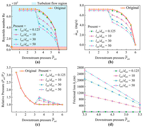
Figure 10.
Effects of length-to-diameter ratio on micro-orifice performance: (a) Reynolds number versus length-to-diameter ratio; (b) relative pressure versus length-to-diameter ratio; (c) mass flow rate versus length-to-diameter ratio; (d) frictional loss versus length-to-diameter ratio.
The critical Reynolds number (Rec) is calculated to be 532.8 at dori = 0.08 mm. As shown in Figure 10a, turbulent flow dominates the gas supply through the micro-orifices. Under these conditions, turbulent shear stress between fluid layers significantly amplifies energy dissipation due to wall roughness effects. The influence of the length-to-diameter ratio on the mass flow rate and the relative pressure between the inlet and the outlet is illustrated in Figure 10b and Figure 10c, respectively. The results indicate that when the downstream pressure of the micro-orifices exceeds the critical pressure (βκ × ps), the mass flow rate begins to decrease, whereas the relative pressure remains unchanged in the original model without frictional loss. In contrast, when frictional loss is considered, the inlet pressure increases as the length-to-diameter ratio increases to compensate for the pressure drop, and the mass flow rate decreases proportionally. Furthermore, both the mass flow rate and the relative pressure closely match those predicted by the original model without frictional loss at a length-to-diameter ratio of 0.125, because frictional loss becomes negligible at this ratio, as shown in Figure 10d.
Figure 11 illustrates the influence of micro-orifice relative roughness on the mass flow rate, relative pressure, and Reynolds number at lori/dori = 10. The results show that as the relative roughness increases, the mass flow rate decreases due to enhanced frictional loss. Moreover, the effective throttling area decreases with increasing relative roughness, which can be approximated by
where kori = 1.0 denotes an empirical correction coefficient. Consequently, when the downstream pressure falls below the critical threshold, the mass flow rate is inversely related to the relative roughness, while being independent of the micro-orifice relative pressure.
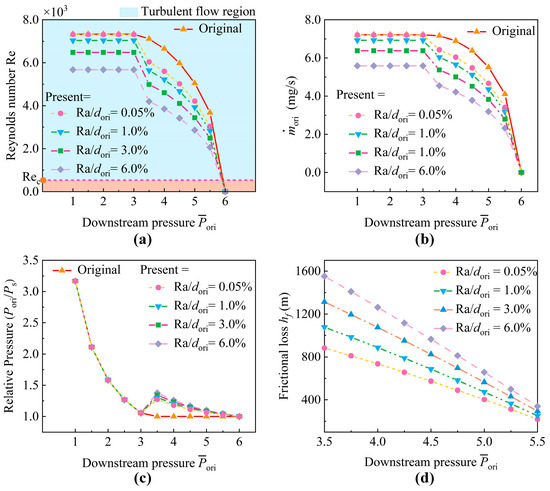
Figure 11.
Effects of relative roughness on micro-orifice performance: (a) Reynolds number versus relative roughness; (b) relative pressure versus relative roughness; (c) mass flow rate versus relative roughness; (d) frictional loss versus relative roughness.
The relationships between the mass flow rate and the length-to-diameter ratio of micro-orifices at Ra/dori = 0.05% are illustrated in Figure 12. It can be observed that as the length-to-diameter ratio increases, the relative error in the mass flow rates calculated using the proposed model with frictional loss and the conventional model without frictional loss also increases. Notably, when the micro-orifice length-to-diameter ratio is less than 4, the reduction in the mass flow rate is below 5% at Ra/dori = 0.05%.
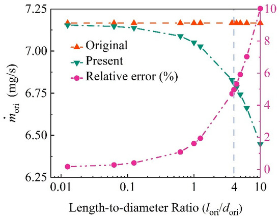
Figure 12.
Mass flow rate and relative error versus length-to-diameter ratio at relative roughness of 0.05%.
4.2. Effects of Frictional Loss on the Lubrication Performance of ACBMOs
In this section, the effects of micro-orifice frictional loss on the lubrication performance of ACBMOs are investigated, focusing on the pressure distribution in the bearing clearance and the load capacity of ACBMOs. The micro-orifice diameter is set to dori = 0.1 mm, and the remaining parameters can be found in Table 3.
Table 3.
Mathematical parameters governing in this segment.
Figure 13 demonstrates the influence of the micro-orifice length-to-diameter ratio on the pressure distribution of ACBMOs at a fixed relative roughness (Ra/dori = 1.0%). The analysis shows that the pressure within the micro-orifices decreases as the length-to-diameter ratio increases, particularly when the pressure ratio exceeds the critical ratio βκ. At a ratio lori/dori = 50, the maximum pressure reduction reaches 12.06%, as shown in Figure 13c. However, when the downstream pressure falls below the critical pressure, pressure perturbations cannot propagate upstream to affect the outflow characteristics. Therefore, under sonic flow conditions, the mass flow rate remains maximized, governed solely by the effective area of the micro-orifices and independent of their relative pressure, as illustrated in Figure 13b.
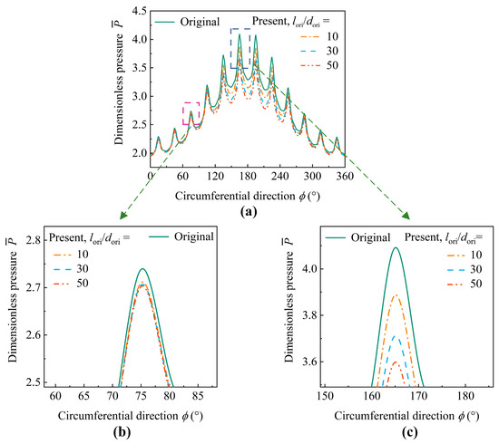
Figure 13.
Effects of micro-orifice length-to-diameter ratio: (a) pressure distribution in the circumferential direction; (b,c) enlarged view of the marked region in (a).
Figure 14 compares the pressure distributions predicted by the proposed model (with frictional loss) and the original model (without frictional loss) at a length-to-diameter ratio of lori/dori = 10 and further illustrates the effects of micro-orifice relative roughness on lubrication performance. It can be observed that the circumferential pressure predicted by the model with frictional loss, within the angular range ϕ = 100–260°, is lower than that predicted by the model without frictional loss. This discrepancy increases as the downstream pressure at these micro-orifices exceeds the critical pressure. Moreover, as relative roughness increases, intensified micro-orifice friction and turbulent shear stress reduce the static flow rates, culminating in a maximum pressure reduction of 10.97%, as shown in Figure 14c.
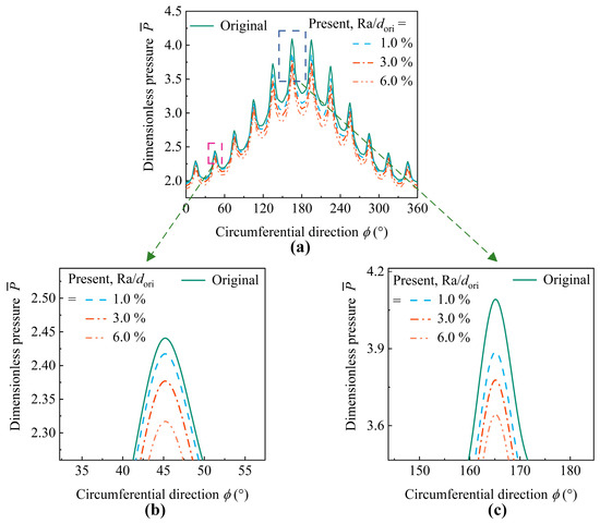
Figure 14.
Effects of micro-orifice relative roughness: (a) pressure distribution in the circumferential direction; (b,c) enlarged view of the marked region in (a).
Conversely, although the mass flow rate is unaffected by downstream pressure under subcritical conditions due to sonic flow, the effective throttling area decreases as the micro-orifice relative roughness increases. Consequently, the diminishing mass flow weakens the hydrostatic support, resulting in a maximum pressure reduction of 5.07% compared to the original models without frictional loss.
Figure 15 illustrates that the radial and axial load capacities of the ACBMOs are affected by the relative roughness of the micro-orifices at different bearing numbers. The results demonstrate that both the Fhr and FhZ decrease as the micro-orifice relative roughness increases when accounting for the frictional loss. Moreover, this reduction progressively intensifies with increasing relative roughness, with the maximum reduction in Fhr reaching 15.8%, as shown in Figure 15a. The reason is that increasing the micro-orifice relative roughness leads to higher frictional loss and lower mass flow rates.
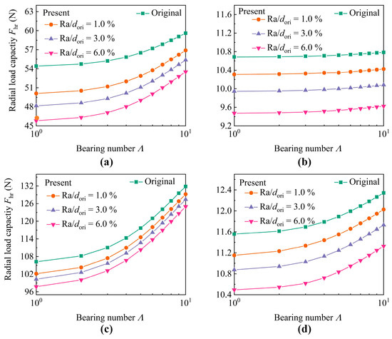
Figure 15.
Load capacity versus bearing number with different relative roughness values: (a) Fhr at εr = 0.3, (b) FhZ at εr = 0.3, (c) Fhr at εr = 0.6, (d) FhZ at εr = 0.6.
Notably, as the bearing number increases (Figure 16), the maximum radial load reduction at an eccentricity ratio (εr = 0.3) decreases from 15.8% to 10.2%. This attenuation is attributed to the shift in the dominant load support mechanism from hydrostatic to hydrodynamic effects. At low speed, the load capacity strongly depends on external gas supply pressure, whereas hydrodynamic-dominated regimes are less sensitive to micro-orifice frictional loss. Consequently, enhanced hydrodynamic effects at higher bearing numbers mitigate the detrimental impact of the frictional loss on load capacity.
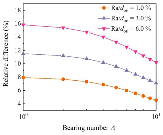
Figure 16.
Relative difference in load capacity versus bearing number under different relative roughness values.
4.3. Effects of Frictional Loss on Nonlinear Behaviors and Stability
The nonlinear behaviors of the ACBMO–rotor system with frictional loss are investigated in this section. The unbalance mreu is located at node 16 and node 31, as shown in Figure 5. The nonlinear response is the ACBMO(R) at node 25. The remaining parameters listed in Table 4 are used by default.
Table 4.
Mathematical parameters of ACBMO–rotor system governing in this segment.
Figure 17 presents bifurcation diagrams for varying micro-orifice length-to-diameter ratios and relative roughness. Based on frequency characteristics and shaft orbits, rotor operational regimes are categorized into three ranges: stable, unstable, and failure. As shown in Figure 17a, when the rotational speed is below 213.0 krpm, the orbits exhibit synchronous periodic motion (Figure 18(a.1)), indicating stable operation characterized solely by fundamental frequency components in the amplitude spectrum. However, upon reaching 213.0k rpm, frequency spectrum analysis (Figure 18(c.2)) reveals a 0.5× sub-synchronous component, which signifies that the system is undergoing period-2 motion, and the transition from the stable state to the unstable state occurs. As the rotational speed increases further to 225.0k rpm, rotor touchdown occurs due to the excessive amplitude of the limit cycle.
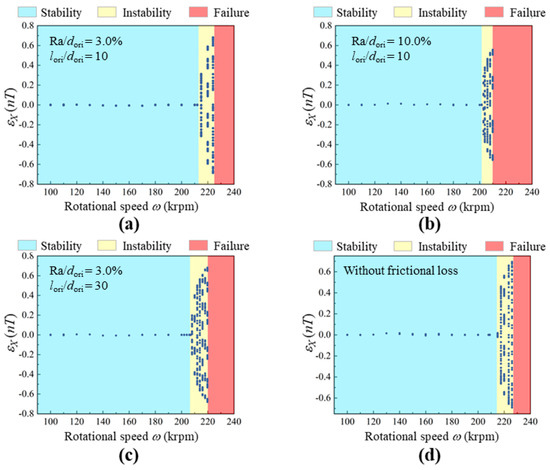
Figure 17.
Bifurcation diagrams of ACBMOs(R) versus rotational speed: (a) Ra/dori = 3.0% and lori/dori = 10, (b) Ra/dori = 10.0% and lori/dori = 10, (c) Ra/dori = 3.0% and lori/dori = 30, (d) without frictional loss.
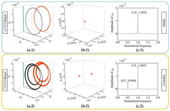
Figure 18.
The nonlinear behaviors of the ACBMO–rotor system at ω = 212.8 krpm and 213.0 krpm: (a.1,a.2) rotor orbits, (b.1,b.2) Poincaré maps, (c.1,c.2) amplitude spectra.
Comparing Figure 17a and Figure 17d, the proposed ACBMO model with frictional loss predicts lower critical instability and failure speeds than the model without frictional loss, with reductions of 0.84% and 6.06%, respectively. Furthermore, increasing the micro-orifice relative roughness and length-to-diameter ratio further lowers these thresholds. Specifically, the critical instability speed in Figure 17b and Figure 17c decreases by 5.45% and 3.0%, respectively, relative to Figure 17a. Meanwhile, the critical failure speed in Figure 17b and Figure 17c declines by 6.67% and 2.22%, respectively.
Figure 19 and Figure 20 demonstrate the effects of micro-orifice frictional loss on nonlinear behaviors at 210 krpm. Figure 19 reveals that, at a length-to-diameter ratio of 10 and a relative roughness of 3.0%, the fundamental amplitude of the ACBMO model with frictional loss slightly exceeds that of the original model without frictional loss, which indicates that frictional loss has only a minor effect on nonlinear behavior under these operation conditions. However, when the length-to-diameter of the micro-orifices increases to 30 (Figure 20a), nonlinearities dominate the system dynamics, and self-excited vibration occurs as the static pressure decreases. A sub-synchronous component can be detected in the frequency spectrum, with an amplitude substantially higher than that of the 1× fundamental frequency. Furthermore, when the length-to-diameter ratio remains at 10 but the relative roughness of the micro-orifices increases to 10%, the time-domain response exhibits divergent growth, culminating in rotor–bearing sleeve contact at t = 4.94 ms and eventual system failure.
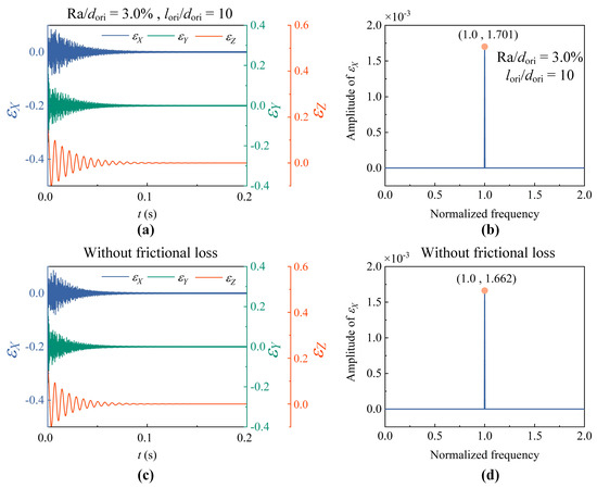
Figure 19.
Time-domain responses of εX, εY and εZ at 210 krpm and their corresponding amplitude spectra: (a,b) Ra/dori = 3.0% and lori/dori = 10, (c,d) without frictional loss.
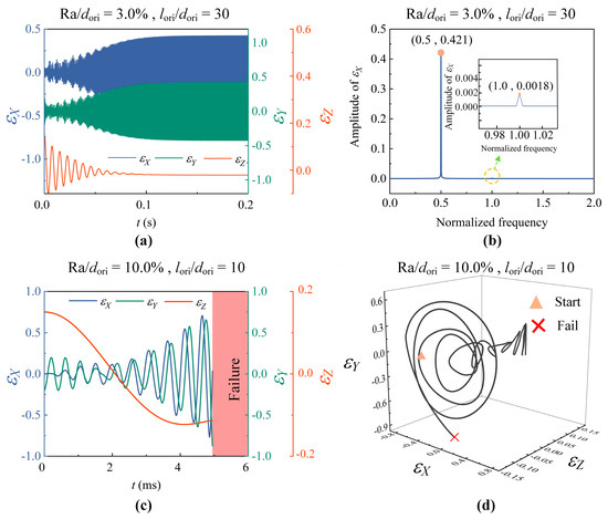
Figure 20.
Time-domain responses of εX, εY and εZ at 210 krpm and their corresponding amplitude spectra: (a,b) Ra/dori = 3.0% and lori/dori = 30, (c,d) Ra/dori = 10.0% and lori/dori = 10.
5. Conclusions
In this paper, a model of an aerostatic conical bearing with micro-orifices, incorporating frictional loss, is established, and the effects of micro-orifice relative roughness and length-to-diameter ratio on flow characteristics, pressure distribution, and load capacity of the ACBMO are systematically analyzed. Furthermore, a flexible aerostatic conical bearing–rotor model incorporating frictional loss is developed to elucidate its impact on ultra-high-speed rotor stability. The principal conclusions are summarized as follows:
(1) Due to the significantly reduced critical Reynolds number in micro-orifices, the mass gas flow rate distinctly declines as a result of turbulent shear stress and micro-orifice wall friction. This reduction exceeds 5% when the micro-orifice length-to-diameter ratio is greater than 4. Concurrently, an increase in micro-orifice inlet pressure compensates for the pressure drop caused by frictional loss.
(2) The load capacity of the ACBMOs decreases as the micro-orifice relative roughness and length-to-diameter ratio increase, due to reduced static pressure from the external gas source. However, as the bearing number increases, the dominant load-support mechanism shifts from hydrostatic to hydrodynamic effects, progressively reducing the relative impact of micro-orifice frictional loss on the load capacity.
(3) Compared to the conventional model without micro-orifice frictional loss, the present model incorporating frictional loss predicts an earlier transition from stability to instability and eventual failure as the rotational speed increases. Furthermore, under the same rotational speed, the relative roughness and length-to-diameter ratio of the micro-orifices significantly influence the dynamic behavior of the ACBMO–rotor system, making it more susceptible to instability as these parameters increase.
Author Contributions
Conceptualization, Q.H. and X.W.; methodology, Q.H. and X.W.; software, Q.H.; validation, Q.H. and C.Z.; formal analysis, Q.H.; investigation, Q.H.; resources, X.W.; data curation, Q.H. and C.Z.; writing—original draft preparation, Q.H. and X.W.; writing—review and editing X.W.; visualization, Q.H. and C.Z.; supervision, X.W.; project administration, X.W.; funding acquisition, X.W. All authors have read and agreed to the published version of the manuscript.
Funding
This research was funded by the National Key Research and Development Program of China (No. 2022YFB3402701) and the National Natural Science Foundation of China (No. 52375165).
Data Availability Statement
The original contributions presented in this study are included in the article. Further inquiries can be directed to the corresponding author.
Conflicts of Interest
The authors declare that the research was conducted without any commercial or financial relationships that could be construed as a potential conflict of interest.
Correction Statement
This article has been republished with a minor correction to the Data Availability Statement. This change does not affect the scientific content of the article.
Nomenclature
| R | Bearing radius, m |
| r, ϕ | Conical coordinates, m and ° |
| t | Time, s |
| u | Node displacement of rotor, m |
| α | Semi-cone angle, ° |
| Ra | Mean bearing radius, m |
| p | Pressure, Pa |
| ps | Supply pressure, Pa |
| Er | Young’s modulus of rotor, Pa |
| νr | Poisson’s ratio of rotor |
| Ts | Supply temperature, K |
| pin | Inlet pressure of orifices, Pa |
| pori | Downstream pressure of orifices, Pa |
| lori | Length of orifices, m |
| dori | Diameter of orifices, m |
| Aori | Area of orifices, m2 |
| Aeff | Effective area of orifices, m2 |
| τW | Shear stress, Pa |
| hf | Frictional loss, m |
| Ma | Mach number |
| ug | Velocity of gas flow, m/s |
| Cd | Discharge coefficient |
| κ | Ratio of specific heat of gas |
| X, Y, Z | Cartesian coordinates, m |
| in | Inlet mass inflow rate, kg/s |
| ori | Outlet mass inflow rate, kg/s |
| *ori | *ori = Cd × ori |
| er | Radial eccentricity, m |
| V | Average velocity of flow, m/s |
| h | Film thickness, m |
| κ1,κ2 | Experiment coefficients |
| τturb | Shear stress of turbulent flow, Pa |
| l0 | Distance between orifices and edges, m |
| L | Bearing length, m |
| δk | Kronecker function |
| mr | Rotor mass, kg |
| Ra | Average roughness of orifice, m |
| pa | Ambient pressure, Pa |
| βκ | Critical pressure ratio |
| R1, R2 | Bearing radius of bearing edges, m |
| Re | Reynolds numbers |
| Gr | Shear modulus of rotor, Pa |
| Dimensionless r, | |
| c0 | Clearance, m |
| τ | Dimensionless t, τ = ωt |
| ρ | Air density, kg/m3 |
| ρr | Rotor density, kg/m3 |
| ω | Rotational speed, rad/s |
| Dimensionless p, = p/pa | |
| Λ | Bearing number |
| ψ | Axial coordinate after conformal map |
| ζ | Conformal map coefficient |
| Fhr | Bearing radial load capacity, N |
| Fer | Radial external force, N |
| f | Friction factor |
| u* | Shear velocity of gas flow, s−1 |
| Ai | Rotor area of section i, m2 |
| Φi | Φi = 12ErId,i/(ks,iGrAiL2i) |
| Rs1, Rs2 | Outer and inner radius of rotor, m |
| Id,i | Inertia moment of section i, m4 |
| Li | Rotor length of section i, m |
| Dimensionless h, | |
| ks,i | Shear coefficient of section i |
| No | Number of orifices |
| μ | Air dynamic viscosity, Pa∙s |
| τ | Non-dimensional time variable |
| eu | Rotating unbalance offset, m |
| kori | Coefficient of experience |
| c | Sonic speed, m/s |
| lmix | Prandtl mixing length, m |
| Qori | Volume inflow rate, m3/s |
| Qo | The gas mass flow factor of the orifices |
| X, Y, Z | Displacement vector on X, Y, Z axis |
| MXY | Radial mass matrix |
| MZ | Axial mass matrix |
| mR,i | Element rotational mass matrix |
| mT,i | Element translational mass matrix |
| mZ,i | Element axial mass matrix |
| KXY | Radial stiffness matrix |
| KZ | Axial stiffness matrix |
| ke,i | Element stiffness matrix |
| kZ,i | Element axial stiffness matrix |
| GXY | Radial gyroscopic matrix |
Appendix A
The element translational mass matrix mT,i is given as
where the elements in mT,i are given as
where . For hollow sections, the cross-sectional area Ai, the moment of inertia Id,i, and the shear coefficients ks,i of any section i are defined as follows:
The element rotational mass matrix mR,i is given as
where the elements in mR,i are given as
The element stiffness matrix ke,i is given as
The element axial mass matrix mZ,i and element axial stiffness matrix kZ,i are given as
References
- An, C.H.; Zhang, Y.; Xu, Q.; Zhang, F.H.; Zhang, J.F.; Zhang, L.J.; Wang, J.H. Modeling of dynamic characteristic of the aerostatic bearing spindle in an ultra-precision fly cutting machine. Int. J. Mach. Tools Manuf. 2010, 50, 374–385. [Google Scholar] [CrossRef]
- Zhang, G.; Huang, M.; Chen, G.; Li, J.; Liu, Y.; He, J.; Zheng, Y.; Tang, S.; Cui, H. Design and optimization of fluid lubricated bearings operated with extreme working performances—A comprehensive review. Int. J. Extrem. Manuf. 2024, 6, 022010. [Google Scholar] [CrossRef]
- Feng, K.; Wang, P.; Zhang, Y.; Hou, W.; Li, W.; Wang, J.; Cui, H. Novel 3-D printed aerostatic bearings for the improvement of stability: Theoretical predictions and experimental measurements. Tribol. Int. 2021, 163, 107149. [Google Scholar] [CrossRef]
- Wu, Y.; Li, C.; Li, J.; Du, J. Lubrication mechanism and characteristics of aerostatic bearing with close-spaced micro holes. Tribol. Int. 2024, 192, 109278. [Google Scholar] [CrossRef]
- Gao, S.; Jiang, T.; Li, Z.; Yang, H.; Zhu, M.; Shang, Y.; Song, L.; Lu, L.; Gao, Q.; Zhang, H. Performance Investigation of the Micro-Hole High-Speed Aerostatic Thrust Bearing Based on the Finite Element Method. Machines 2025, 13, 477. [Google Scholar] [CrossRef]
- Talukder, H.M.; Stowell, T.B. Pneumatic hammer in an externally pressurized orifice-compensated air journal bearing. Tribol. Int. 2003, 36, 585–591. [Google Scholar] [CrossRef]
- Chen, X.; Chen, H.; Luo, X.; Ye, Y.; Hu, Y.; Xu, J. Air Vortices and Nano-Vibration of Aerostatic Bearings. Tribol. Lett. 2011, 42, 179–183. [Google Scholar] [CrossRef]
- Chen, X.; Chen, H.; Zhu, J.; Jiang, W. Vortex suppression and nano-vibration reduction of aerostatic bearings by arrayed microhole restrictors. J. Vib. Control. 2016, 23, 842–852. [Google Scholar] [CrossRef]
- Mohiuddin Mala, G.; Li, D. Flow characteristics of water in microtubes. Int. J. Heat Fluid Flow 1999, 20, 142–148. [Google Scholar] [CrossRef]
- Chen, Q.L.; Wu, K.J.; He, C.H. Investigation on liquid flow characteristics in microtubes. AIChE J. 2014, 61, 718–735. [Google Scholar] [CrossRef]
- Yao, Z.; Hao, P.; Zhang, X. Effects of gas compressibility and surface roughness on the flow in microfluidic devices. Sci. China Phys. Mech. Astron. 2011, 54, 711–715. [Google Scholar] [CrossRef]
- Tang, G.H.; Li, Z.; He, Y.L.; Tao, W.Q. Experimental study of compressibility, roughness and rarefaction influences on microchannel flow. Int. J. Heat Mass Transf. 2007, 50, 2282–2295. [Google Scholar] [CrossRef]
- Li, Y.; Zhang, Z.; Ji, Y.; Wang, L.; Li, D. Influence of surface roughness on the fluid flow in microchannel. J. Phys. Conf. Ser. 2024, 2740, 012059. [Google Scholar] [CrossRef]
- Hu, H.; Feng, M.; Ren, T. Study on the performance of novel gas foil conical bearings. Proc. Inst. Mech. Eng. Part J J. Eng. Tribol. 2020, 235, 883–900. [Google Scholar] [CrossRef]
- Liu, W.; Bättig, P.; Wagner, P.H.; Schiffmann, J. Nonlinear study on a rigid rotor supported by herringbone grooved gas bearings: Theory and validation. Mech. Syst. Signal Process. 2021, 146, 106983. [Google Scholar] [CrossRef]
- An, L.; Wang, W.; Wang, C. Dynamic modeling and analysis of high-speed aerostatic journal bearing-rotor system with recess. Tribol. Int. 2023, 187, 108686. [Google Scholar] [CrossRef]
- Chen, P.; Ding, J.; Zhuang, H.; Chang, Y. A novel method for studying fluid-solid interaction problems of the rotor system in air bearings with manufacturing errors. Mech. Syst. Signal Process. 2023, 202, 110709. [Google Scholar] [CrossRef]
- Zheng, C.; Wang, X.; Zhang, X.; Wang, C.; Han, Q. Three-dimensional nonlinear behaviors and stability analysis of high-speed aerostatic conical bearing-rotor system. Nonlinear Dyn. 2025, 113, 17613–17636. [Google Scholar] [CrossRef]
- Belforte, G.; Raparelli, T.; Viktorov, V.; Trivella, A. Discharge coefficients of orifice-type restrictor for aerostatic bearings. Tribol. Int. 2007, 40, 512–521. [Google Scholar] [CrossRef]
- Li, D.; Yang, R.; Cao, H.; Yao, F.; Shen, C.; Zhang, C.; Wu, S. Experimental Study on Gas Flow in a Rough Microchannel. Front. Energy Res. 2022, 10, 863733. [Google Scholar] [CrossRef]
- Morini, G.L.; Lorenzini, M.; Salvigni, S.; Spiga, M. Thermal performance of silicon micro heat-sinks with electrokinetically-driven flows. A preliminary version of this paper was presented at ICMM05: Third International Conference on Microchannels and Minichannels, held at University of Toronto, June 13–15, 2005, organized by S.G. Kandlikar and M. Kawaji, CD-ROM Proceedings. Int. J. Therm. Sci. 2006, 45, 955–961. [Google Scholar] [CrossRef]
- Eckert, M. Turbulence Research in the 1920s and 1930s between Mathematics, Physics, and Engineering. Sci. Context 2018, 31, 381–404. [Google Scholar] [CrossRef]
- Zeghadnia, L.; Robert, J.L.; Achour, B. Explicit solutions for turbulent flow friction factor: A review, assessment and approaches classification. Ain Shams Eng. J. 2019, 10, 243–252. [Google Scholar] [CrossRef]
- Chen, W.J.; Gunter, E. Dynamics of Rotor-Bearing Systems—Ch. 5 Shaft Finite Element Equations; Chen, W.J., Gunter, E.J., Eds.; Trafford Publishing: Bloomington, IN, USA, 2023; p. 155. [Google Scholar]
- Nelson, H.D. A finite rotating shaft element using Timoshenko beam theory. J. Mech. Des. Trans. ASME 1980, 102, 793–803. [Google Scholar] [CrossRef]
- Nelson, H.D.; McVaugh, J.M. The dynamics of rotor-bearing systems using finite elements. J. Manuf. Sci. Eng. Trans. ASME 1976, 98, 593–600. [Google Scholar] [CrossRef]
- Zhang, J.; Deng, Z.; Zhang, K.; Jin, H.; Yuan, T.; Chen, C.; Su, Z.; Cao, Y.; Xie, Z.; Wu, D.; et al. The Influences of Different Parameters on the Static and Dynamic Performances of the Aerostatic Bearing. Lubricants 2023, 11, 130. [Google Scholar] [CrossRef]
- Yang, P.; Zhu, K.-Q.; Wang, X.-L. On the non-linear stability of self-acting gas journal bearings. Tribol. Int. 2009, 42, 71–76. [Google Scholar] [CrossRef]


Disclaimer/Publisher’s Note: The statements, opinions and data contained in all publications are solely those of the individual author(s) and contributor(s) and not of MDPI and/or the editor(s). MDPI and/or the editor(s) disclaim responsibility for any injury to people or property resulting from any ideas, methods, instructions or products referred to in the content. |
© 2025 by the authors. Licensee MDPI, Basel, Switzerland. This article is an open access article distributed under the terms and conditions of the Creative Commons Attribution (CC BY) license (https://creativecommons.org/licenses/by/4.0/).