Fault Diagnosis of Rolling Bearing Based on Spectrum-Adaptive Convolution and Interactive Attention Mechanism

Abstract

With the development of artificial intelligence technology, intelligent fault diagnosis methods based on deep learning have received extensive attention. Among them, convolutional neural network (CNN) has been widely applied in the fault diagnosis of rolling bearings due to its strong feature extraction ability. However, traditional CNN models still have deficiencies in the extraction of early weak fault features and the suppression of high noise. In response to these problems, this paper proposes a convolutional neural network (SAWCA-net) that integrates spectrum-guided dynamic variable-width convolutional kernels and dynamic interactive time-domain–channel attention mechanisms. In this model, the spectrum-adaptive wide convolution is introduced. Combined with the time-domain and frequency-domain statistical characteristics of the input signal, the receptive field of the convolution kernel is adaptively adjusted, and the sampling position is dynamically adjusted, thereby enhancing the model’s modeling ability for periodic weak faults in complex non-stationary vibration signals and improving its anti-noise performance. Meanwhile, the dynamic time–channel attention module was designed to achieve the collaborative modeling of the time-domain periodic structure and the feature dependency between channels, improve the feature utilization efficiency, and suppress redundant interference. The experimental results show that the fault diagnosis accuracy rates of SAWCA-Net on the bearing datasets of Case Western Reserve University (CWRU) and Xi’an Jiaotong University (XJTU-SY) reach 99.15% and 99.64%, respectively, which are superior to the comparison models and have strong generalization and robustness. The visualization results of t-distributed random neighbor embedding (t-SNE) further verified its good feature separability and classification ability.

1. Introduction

Rolling bearings are essential components in mechanical equipment. Under complex conditions such as high load, high speed, and high temperature, they are prone to faults like wear and cracking [1,2]. These faults can cause equipment shutdowns or even safety incidents, leading to high maintenance and replacement costs. Therefore, real-time online monitoring, timely extraction of fault features, and accurate status identification are key to ensuring stable equipment operation [3,4,5].

Vibration signal analysis is a common approach for bearing fault diagnosis. Methods such as empirical mode decomposition, wavelet transform, sparse decomposition, and Fourier transform [6,7,8,9] can extract characteristic parameters from the time, frequency, and time–frequency domains to determine bearing operating conditions and fault types. Although effective under certain conditions, these methods depend heavily on parameter tuning and expert experience. Their performance often degrades under complex or changing operating conditions, making it difficult to extract stable fault features.

With the development of machine learning, methods such as k-nearest neighbor (KNN), support vector machine (SVM), random forest (RF), and back propagation neural network (BP) have been applied to bearing fault diagnosis [10,11]. These methods work well in small-sample cases but rely on manually designed features, making their performance sensitive to feature quality. They may also face challenges in efficiency and generalization when dealing with large, high-dimensional datasets.

Facing the challenges of the surging volume of industrial monitoring data and the increasing complexity of equipment structures, deep learning technology, with its advantages of automatic feature learning and nonlinear modeling, has gradually become a research hotspot [12,13]. Deep learning can directly mine effective information from the original signal, reducing the reliance on artificial feature design. Its multi-level network structure is suitable for processing high-dimensional and diverse large-scale data, and the end-to-end modeling approach also enhances the efficiency and accuracy of diagnosis.

Specifically, the multi-entropy screening and optimization temporal convolutional network (MESO-TCN) method proposed by Gao et al. [14] combines empirical mode decomposition with the hybrid entropy criterion. It extracts fault features at different time scales through multi-scale expanded convolutional networks and achieves adaptive adjustment of key hyperparameters with the aid of an improved optimization algorithm. This has enhanced the generalization ability and robustness of the model. The multi-scale convolutional neural network designed by Wang et al. [15] extracts multi-level fault features, enhancing feature representation and improving diagnostic accuracy. The hybrid model proposed by Han et al. [16] that integrates convolutional neural network (CNN), long short-term memory network (LSTM), and gated recurrent unit (GRU) possesses both spatial and temporal series feature extraction capabilities, can capture long and short-term dependency information in signals, and significantly enhances the stability of the model in complex environments. Jiang et al. [17] utilized the lightweight ShuffleNetV2 structure and combined the variational mode decomposition (VMD) and fast Kurtograph (FK) algorithms to achieve efficient signal denoising and feature extraction, which is particularly suitable for resource-constrained industrial application scenarios. In addition, Misbah et al. [18] developed a hybrid deep learning network model based on multi-scale convolutional neural networks, aiming to accurately extract fault features.

Although the above-mentioned methods have made significant progress in feature extraction and fault classification, they still face challenges in practical and complex applications. Especially in harsh environments and complex transmission paths, the early fault signals are weak and easily masked by noise, resulting in a large amount of interference information in the signals. Most models focus on local feature extraction and lack effective modeling of the global temporal structure of the signal, making it difficult to accurately capture subtle periodic changes and affecting the recognition accuracy and generalization ability. Meanwhile, in a strong noise environment, the model has difficulty distinguishing between effective and redundant features, which reduces the diagnostic stability. Therefore, designing deep learning models with stronger robustness and global feature learning capabilities remains an important development direction in the field of rolling bearing fault diagnosis.

To address these issues, this paper proposes the spectrum adaptive wide convolution and attention network (SAWCA-Net) for rolling bearing fault diagnosis. The main contributions are as follows:

(1) We design a spectrum-adaptive wide convolution module that integrates spectral statistical features. This module dynamically adjusts the receptive field range and sampling position of the convolution kernel based on the time-domain and frequency-domain statistics of the input signal (such as energy, kurtosis, spectral entropy, principal frequency amplitude, etc.), achieving adaptive modeling of signals of different scales and structures. This module can enhance the model’s ability to identify weak periodic fault features and non-stationary disturbances, effectively suppress high-frequency noise at the front end, and improve the quality of low-level feature expression.

(2) We construct the dynamic time–channel attention module. This module automatically adjusts the importance distribution of multi-dimensional features by introducing an interactive feedback mechanism between the time and channel branches, strengthens the modeling of key periodic structures and feature dependencies between channels, and effectively enhances the overall feature utilization efficiency and fault discrimination capability.

(3) Under the condition of strong noise interference, the proposed method shows strong robustness and generalization ability. In this paper, comparative experiments are carried out on two public datasets, Case Western Reserve University (CWRU) and Xi’an Jiaotong University (XJTU-SY), and the fault identification performance of the model under complex working conditions is verified.

2. The Proposed Method

2.1. SAWCA-Net Framework

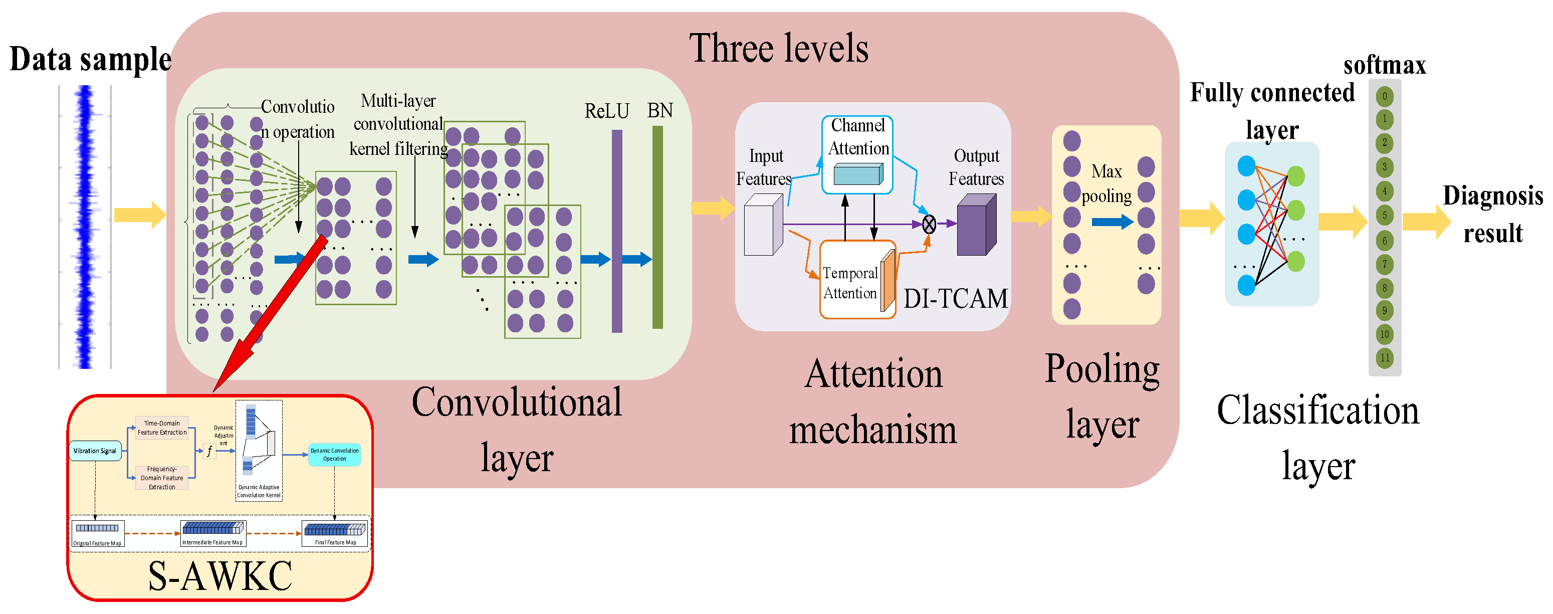
The spectrum-adaptive wide convolution and attention network (SAWCA-Net) proposed in this paper mainly consists of an input layer, a convolutional layer, an efficient time channel attention mechanism module, a pooling layer, and a fully connected layer. Among them, the input layer is used for preprocessing the data, and the hidden layer is alternately composed of multiple convolutional layers, attention mechanism modules, and pooling layers, outputting the final two-dimensional feature map. It is expanded into a one-dimensional feature vector and connected to the fully connected layer, forming a classifier with the output layer. The softmax function is used in the output layer to output the probability distribution of multiple categories. Its structure is shown in Figure 1.

2.2. S-AWKC Module

In the proposed SAWCA-Net model, the convolution layer, as a front-end feature extraction module, is responsible for extracting key time-series structural features from complex and non-stationary one-dimensional vibration signals. The traditional CNN usually adopts a fixed-size convolutional kernel. Although it has strong local pattern recognition ability, its receptive field is limited, and it is difficult to capture the periodic weak fault features in the signal, especially in the environment of high noise interference, which is prone to insufficient feature coverage or over-fitting of local pseudo-features, thus limiting the diagnostic accuracy and the generalization performance of the model.

In order to solve the above problems, this paper designs a spectrum-guided adaptive wide kernel convolution (S-AWKC), which integrates spectrum statistics. The module comprehensively utilizes the statistical characteristics of the input signal in time domain and frequency domain (such as energy, kurtosis, spectral entropy, and amplitude of main frequency) to dynamically adjust the width of the receptive field of the convolution kernel and guides the shift of sampling position based on the spectral structure so as to realize the adaptive sensing and positioning ability of the convolution kernel at different time positions. This strategy not only improves the modeling ability of the model for multi-scale periodic structures but also enhances the stability of feature extraction in a background with strong noise. The overall structure of S-AWKC module is shown in Figure 2, which mainly includes the following three parts:

(1) Spectral feature extraction and statistical modeling in spectral domain.

Let the original input signal be x(t), t = 1, 2, …; T is transformed into the frequency domain by using the fast Fourier transform (FFT) to obtain the spectral representation X(f). Extract multiple representative statistical features in the frequency domain to form a spectral feature vector:

$$S=Sta{t}_{spec}(X(f))=[A_{peak},H,f_c,E_s]$$

(1)

Among them, $A_{peak}$ is the amplitude of the main frequency, $H$ is the spectral entropy, $f_c$ is the spectral centroid, and $E_s$ represents the energy in the frequency domain. The definitions of these spectral characteristics follow the common practices of classic textbooks on digital signal processing [19,20] and the literature on vibration fault diagnosis.

(2) Dynamic adjustment strategy of the receptive field

To achieve adaptive convolution kernel scale control, this paper designs a receptive field adjustment function $f(.)$ based on the time-domain and frequency-domain joint statistics. Combining time-domain features (such as energy $E$ and kurtosis $K$) with frequency-domain statistical features, the width k_t of the convolution kernel at each time position is dynamically determined:

$$S_t=[E,H,K,A_{\mathrm{peak}},f_c]$$

(2)

Based on this statistical characteristic, we define the receptive field adjustment function $f(.)$ We can thus dynamically determine the effective width of the convolution kernel:

$$k_t=f(S_t)={\alpha }_1\cdot E+{\alpha }_2\cdot H+{\alpha }_3\cdot K+{\alpha }_4\cdot A_{peak}+{\alpha }_5\cdot f_c$$

(3)

Among them, ${\alpha }_1$ to ${\alpha }_5$ are learnable weight parameters. This weight parameter was initialized using Xavier to ensure the stable transfer of gradients in the early stage of training. This strategy not only expands the receptive field of convolution but also enhances the model’s collaborative perception ability of high-frequency disturbances and low-frequency trends, improving the modeling effect of multi-scale structures. The adaptive receptive field adjustment method proposed in this paper draws on the design concepts of deformable convolution and variable dilation convolution [21]. These weight parameters, together with other parameters of SAWCA-Net, are jointly optimized through supervised learning. The cross-entropy loss between the predicted labels and the real labels is adopted, and the model is trained through the backpropagation algorithm, thereby achieving the improvement of model performance.

(3) Spectral-driven dynamic sampling offset mechanism

To further enhance the parsing ability of convolution for non-stationary local features, the spectrum-adaptive wide convolution module introduces a dynamic offset mechanism based on spectrum. This mechanism predicts the offset ${\Delta }_i(t)$ of each convolution position through a lightweight neural network based on spectral characteristics, achieving flexible adjustment of the sampling position of the convolution kernel:

$$y(t)=\sigma \left({\displaystyle \sum _{i=1}^{k_t}{W}_i}\cdot x(t+{\Delta }_i(t))+b\right)$$

(4)

Among them, $\sigma (.)$ is the activation function, and $W_i$ and $b$ are convolution weights and bias terms, respectively. The frequency spectrum structure of the input signal is considered in the generation of the model, which enhances the positioning ability of the model in different fault feature positions. The learnable offsets in Equation (4) are initialized to zero to start from a standard sampling position. These offsets are defined as differentiable parameters and are jointly optimized with all other network parameters during the end-to-end supervised training process via backpropagation. The optimization uses the same cross-entropy loss function employed for the main classification task, ensuring that the offsets adapt dynamically to input features to enhance the model’s discriminative capability.

In summary, the spectrum-adaptive wide convolution module integrates multiple statistical features in the time domain and frequency domain, jointly completing the dynamic adjustment of the receptive field range of the convolution kernel and the adaptive offset adjustment of the sampling position, significantly enhancing the model’s modeling ability for periodic weak faults and complex spectral disturbances in non-stationary signals. Compared with the traditional fixed convolutional structure, this module has higher flexibility, signal perception ability, and adaptability and can provide stable and high-quality features with recognition value for the subsequent attention mechanism, effectively enhancing the fault recognition performance of the proposed network under complex working conditions.

2.3. Dynamic Interactive Time-Channel Attention Module

To further enhance the recognition ability of the network for the key fault characteristics of rolling bearings in complex backgrounds, this paper designs a dynamic interactive time–channel attention module (DI-TCAM).This module achieves joint optimization and dynamic adjustment of attention weights by establishing a dual-branch interaction mechanism between the time dimension and the channel dimension, enhancing the model’s modeling ability for weak periodic structures and multi-channel collaborative features in non-stationary vibration signals, and improving the stability of feature expression under strong noise interference.

In dynamic time–channel attention, temporal attention and channel attention guide each other, forming a dynamic fusion mechanism during the feature weighting process. Channel attention focuses on depicting the differences in feature contributions of different channels at various time periods, while temporal attention is used to enhance the periodic activation response at critical moments. Through bidirectional feedback and interactive modeling, the module can effectively highlight the timing segments and channel features highly relevant to the fault category, improving the overall feature utilization efficiency and diagnostic accuracy.

(1) Overall architecture

As shown in Figure 3, the DI-TCAM module is composed of a channel attention path and a time attention path. However, unlike the traditional parallel design, this paper introduces an interactive feedback path, achieving dynamic information fusion and iterative calibration between the channel and time dimensions, thereby forming a more recognizable dynamic closed-loop feature recalibration mechanism.

As shown in Figure 3, the dynamic time–channel attention module is composed of a channel attention path and a time attention path. However, unlike the traditional parallel design, this paper introduces an interactive feedback path, achieving dynamic information fusion and iterative calibration between the channel and time dimensions, thereby forming a more recognizable dynamic closed-loop feature recalibration mechanism.

First, we input the feature tensor X ∈ R^B×C×T, where B represents the batch size, C represents the number of channels, and T represents the time step. The input data, after extracting the initial features through the convolutional layer, are input into the dynamic time–channel attention module to start the calculation of interactive attention.

In the channel attention path, the global average pooling (GAP) operation is first adopted to aggregate information along the time dimension to obtain the overall description vector of each channel:

$$s_c={\displaystyle \frac{1}{T}}{\displaystyle \sum _{t=1}^{T}X}[:,:,t]\in {ℝ}^{B\times C}$$

(5)

This step effectively compresses the time series information, enabling the model to focus on the average activation intensity of each channel within the overall time interval. Subsequently, through a set of trainable weight matrices $W_c$ and bias terms $b_c$, combined with a nonlinear activation function, the channel attention weights are mapped out:

$$A_c=\sigma (W_c{\dots }_c+b_c)\in {ℝ}^{B\times C}$$

(6)

Among them, $\sigma (.)$ is the Sigmoid function, which normalizes the weights to the (0, 1) interval. This attention weight represents the importance contribution of different channels to the overall feature learning. This channel attention generation method refers to the implementations of squeeze-and-excitation network (SENet) [22] and convolutional block attention module (CBAM) [23].

Then, based on the channel attention weights, the original feature tensor is weighted and adjusted along the channel dimension to obtain the intermediate feature representation after channel weighting:

$$X_c=A_c\otimes X$$

(7)

Here, $\otimes$ represents the multiplication operation broadcast channel by channel. This channel recalibration operation is the standard practice of the channel attention mechanism [22].

Then, we enter the temporal attention path. First, we perform cross-channel average pooling on the weighted intermediate feature $X_c$ to extract the comprehensive feature description vector in the time dimension:

$$s_t={\displaystyle \frac{1}{C}}{\displaystyle \sum _{c=1}^C{X}_c}[:,c,:]\in {ℝ}^{B\times T}$$

(8)

This step summarizes the multi-channel features at each time step to capture the overall dynamic information of the periodic fluctuations in the vibration signal. After processing with the convolutional mapping weight $W_t$, the bias term $b_t$, and the activation function, the time attention weight is output:

$$A_t=\sigma (W_t{\dots }_t+b_t)\in {ℝ}^{B\times T}$$

(9)

This time attention weight can represent the contribution degree of the vibration signal to fault identification at each time step, effectively guiding the model to focus on the time intervals with obvious periodic fluctuations or prominent abnormal activations. This temporal attention generation process refers to the implementation method of CBAM [23].

(2) Dynamic interactive feedback mechanism

Based on the independent modeling of traditional time and channel attention, the dynamic time–channel attention module innovatively designs a cross-branch dynamic interaction feedback mechanism to achieve information sharing and recursive optimization between the two attention branches.

Specifically, first, the time attention weight is used to reverse-guide the re-correction and update of the channel attention, obtaining the dynamically enhanced channel attention weight:

$$A_c^{\prime }=\sigma (W_c^{\prime }\cdot A_t+b_c^{\prime })$$

(10)

Similarly, the channel attention weight also feeds back to the time attention path and further updates and strengthens the time attention weight:

$$A_t^{\prime }=\sigma (W_t^{\prime }\cdot A_c+b_t^{\prime })$$

(11)

Through the above bidirectional feedback process, dynamic collaborative learning is formed between time and channel features during training, which not only strengthens the modeling of local dependency relationships between channels but also enhances the model’s ability to capture global temporal features of key periodic paragraphs. Especially in dealing with complex and variable early weak failure modes and strong noise interference scenarios, this mechanism can effectively avoid the overfitting problem of local pseudo-features by the single-path attention model and improve the overall stability and robustness of feature recognition.

(3) Feature fusion and output

After obtaining the final dynamic interaction weights $A_c^{\prime }$ and $A_t^{\prime }$, the dynamic time–channel attention module implements dual joint weighting on the input feature tensor to obtain the final output feature tensor:

$$Y=X\cdot (A_c^{\prime }\otimes A_t^{\prime })$$

(12)

Among them, $\otimes$ represents broadcast multiplication; that is, weighted adjustments of feature importance are made, respectively, in the channel dimension and the time dimension. This dual-weighted fusion not only fully retains the weak feature collaboration information between channels but also implements significant amplification on the key period intervals in the fault signal, enabling the model to adaptively focus on high-contribution feature regions during the training process, thereby enhancing the fault discrimination performance and anti-interference ability. The idea of joint weighting of this channel and time is similar to the channel–spatial attention fusion in CBAM [23].

In conclusion, the dynamic time–channel attention module fully integrates the importance information of both temporal and channel two-dimensional features. By introducing a bidirectional interactive feedback mechanism, it achieves dynamic collaborative perception and adaptive weight distribution among multi-dimensional features. This module not only effectively enhances the model’s ability to capture weak periodic fault features but also improves the feature robustness and discriminability in complex and highly noisy environments, providing strong support for the early weak damage identification and stable performance of the rolling bearing fault diagnosis model under complex working conditions.

2.4. Rolling Bearing Fault Diagnosis Process Based on SAWCA-Net

The SAWCA-Net diagnostic process proposed in this paper is shown in Figure 4.

(1) Data preprocessing: Through the data acquisition system, the vibration signals of the rolling bearings in both healthy and faulty states are simultaneously obtained during the test process. First, the original data are cleaned, including eliminating incorrect values, missing values, and outliers, and the amplitude standardization method is used to eliminate dimensional differences under different working conditions. The processed data are proportionally divided into a training set and a test set for model training and performance verification.

(2) Low-level feature extraction (spectrum-adaptive wide convolution module): The preprocessed training samples are first input into this module to extract the key low-level temporal features. This module combines the time-domain and frequency-domain statistics of the input signal (such as energy, spectral entropy, kurtosis, principal frequency amplitude, etc.), dynamically adjusts the receptive field of the convolution kernel, and introduces a deformable convolution mechanism. Based on the learned offsets, it flexibly adjusts the sampling position, thereby enhancing the ability to capture local features in non-stationary signals. After the convolution operation, the ReLU activation function and BN processing are successively carried out, and the initial feature map is output for subsequent use.

(3) Feature enhancement (dynamic time–channel attention module): The initial feature map is sent to the module, which achieves adaptive weighting of the importance of multi-dimensional features through a bidirectional feedback mechanism of time and channel attention. Channel attention recognizes the feature contributions of different channels, while temporal attention strengthens the periodic information in the signal. The two interact and guide each other, enhancing the model’s modeling ability for weak periodic disturbances and multi-channel collaborative features. The weighted feature map output is subjected to max pooling to achieve dimensionality reduction and redundance compression.

(4) Local high-order feature extraction: After dimensionality reduction, the feature map is successively input into two sets of stacked lightweight convolutional modules, and small receptive field convolutional kernels are used to further extract local high-order detail features. Each group of convolution is accompanied by ReLU activation and BN normalization operations to enhance the nonlinear fitting ability and training convergence speed of the model.

(5) Local channel attention embedding: After each set of convolution and pooling operations, a lightweight channel attention mechanism is introduced to further enhance the response of important channels, improve the cross-level feature fusion effect, effectively suppress the accumulation of redundant information, and retain key features.

(6) Fault classification output: The final set of convolutional outputs, after being activated by ReLU, is flattened into one-dimensional feature vectors and sent to the fully connected layer and the softmax classifier to complete the identification of the fault category of the rolling bearing.

3. Case Western Reserve University Dataset

3.1. CWRU Data Introduction

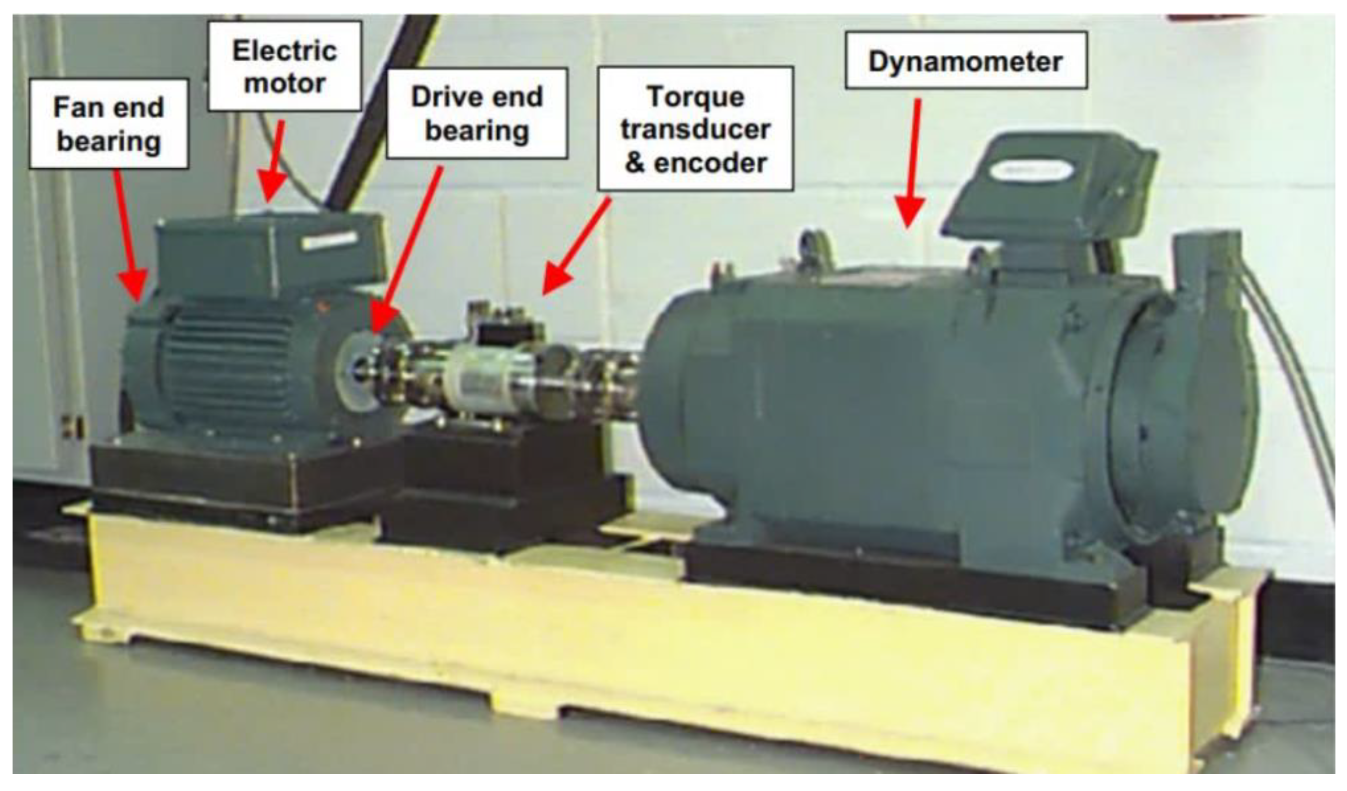
To verify the performance of the proposed model, this paper selects the bearing failure dataset of Case Western Reserve University (CWRU) as the experimental data source. This dataset was collected from a standardized bearing fault test platform and mainly consists of a 2-horsepower induction motor, a coupling, a torque sensor, and a dynamometer. Its structural diagram is shown in Figure 5. The test object is the SKF 6205-2RS deep groove ball bearing, which is installed at the drive end and the fan end of the motor. Acceleration sensors are placed at both positions to collect vibration acceleration signals. The sampling frequency at the drive end is 12 kHz, and at the fan end, it is either 12 kHz or 48 kHz.

To simulate different fault conditions, three defect diameters (0.007 inches, 0.014 inches, and 0.021 inches) were machined on the inner ring, outer ring, and rolling elements of the bearing, and four states—normal, inner ring fault, outer ring fault, and rolling element fault—were set. In the test, the motor operated under three loads of 0 HP, 1 HP, and 2 HP, respectively, corresponding to rotational speeds of 1797 rpm, 1772 rpm, and 1750 rpm. This paper selects a subset of data with a sampling frequency of 12 kHz at the fan end and a defect diameter of 0.007 inches, including three types of faults (inner ring, outer ring, and rolling elements) and normal states, forming a total of 12 operating conditions. Each state is assigned a unique label (0–11).

During the data collection process, vibration signals (totaling 120,000 points) were continuously collected for 10 s in each operating state. Subsequently, 1 s was taken as a sample window, and a 50% sliding window overlap was used for segmentation, thereby obtaining more samples and enhancing data utilization. The final dataset was divided into a training set and a test set in a 70%:30% ratio to ensure that samples from the same time period do not appear in both at the same time, thus avoiding information leakage. The fault categories and their label numbers are shown in

Table 1. Description of each fault type in the CWRU dataset.

Load Condition	Label	Fault Type	Dataset
0 (1797 r/min)	0	Normal	97
	1	Inner Race Fault	105
	2	Rolling Element Fault	118
	3	Outer Race Fault	130
1 (1772 r/min)	4	Normal	98
	5	Inner Race Fault	106
	6	Rolling Element Fault	119
	7	Outer Race Fault	131
2 (1750 r/min)	8	Normal	99
	9	Inner Race Fault	107
	10	Rolling Element Fault	120
	11	Outer Race Fault	132

.

3.2. Comparative Experiment Based on the CWRU Dataset

To evaluate the performance of the proposed method, this study mainly compares it with seven baselines: CNN, LSTM, recurrent neural network (RNN), LeNet, multilayer perceptron (MLP), stacked autoencoder (SAE), and back propagation neural network (BPNN). To ensure fairness, all the above methods were trained with the same settings. The primary evaluation criterion is the diagnostic accuracy rate, defined as the ratio of correctly diagnosed samples to the total number of samples, reflecting the overall performance of the evaluation method. To reduce the influence of randomness, each experiment was conducted three times, and the results are presented in Figure 6 and

Table 2. Experimental results of eight models based on the CWRU dataset.

Model	Max Accuracy (%)	Min Accuracy (%)	Mean Accuracy (%)
SAWCA-Net	99.42	98.96	99.15 ± 0.19
CNN	96.37	95.86	96.13 ± 0.21
LSTM	60.03	52.30	54.93 ± 3.61
RNN	30.34	25.63	27.42 ± 2.08
LeNet	91.84	90.96	91.37 ± 0.36
MLP	85.12	84.49	84.89 ± 0.54
SAE	51.88	48.95	50.85 ± 1.35
BPNN	36.91	35.39	36.36 ± 0.69

.

It can be clearly seen from the results that the method proposed in this paper performs exceptionally well in terms of diagnostic accuracy, with the highest reaching 99.42% and the lowest reaching 98.96%. It is worth noting that even at the lowest diagnostic accuracy rate, the method proposed in this paper still outperforms the highest diagnostic accuracy rates of several other models. Compared with the baselines, SAWCA-Net achieved a significant improvement in diagnostic accuracy. Specifically, compared with these traditional methods, the diagnostic accuracy rates of the proposed network increased by 3.02%, 44.22%, 71.73%, 7.78%, 14.26%, 48.30%, and 62.79, respectively. Moreover, the mean square error of the method proposed in this paper is also the smallest, indicating that this method performs well in terms of stability. Such comprehensive performance further highlights the reliability and effectiveness of the method proposed in this paper as a fault diagnosis model.

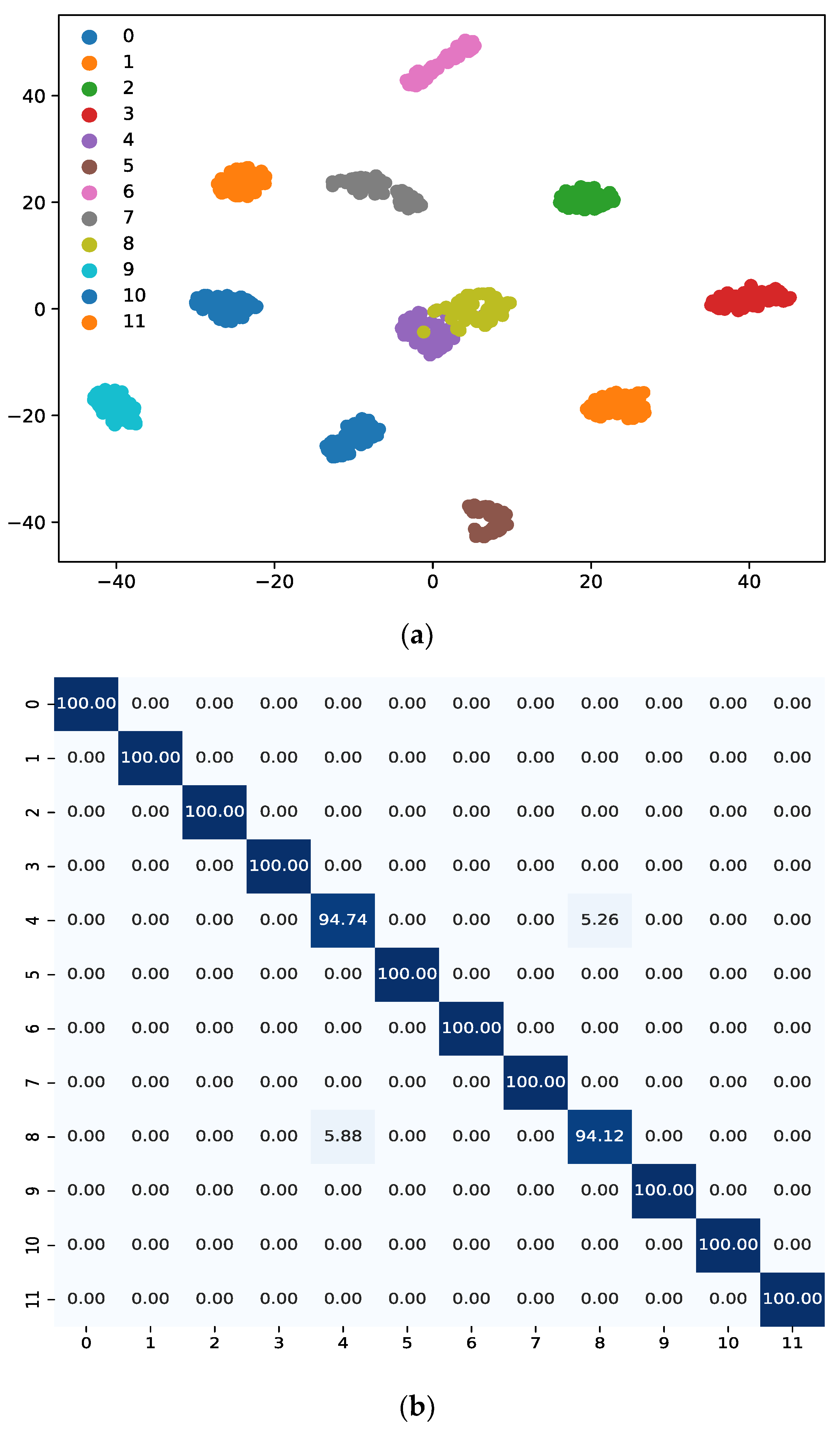
In terms of visual representation, this paper introduces the t-distributed random neighbor embedding (t-SNE) algorithm to reduce the dimension and visualize the feature distribution of the dataset. Different colors correspond to different device health states. Meanwhile, by drawing a confusion matrix, the diagnostic results of the model are visually compared with the actual fault types, where the horizontal axis represents the predicted diagnostic status, and the vertical axis represents the actual fault status. The result is shown in Figure 7.

As can be seen from Figure 7a, except for the boundaries of category 4 and category 8, which are slightly confused, the feature boundaries of the other categories are distinct and have high distinguishability. Figure 7b shows the detailed diagnostic accuracy rates for each category. It can be seen that 5.26% of category 4 was misdiagnosed as category 8, and 5.88% of category 8 was misdiagnosed as category 4. The diagnostic accuracy rate for each category except category 4 and category 8 is 100%, and there are no misdiagnoses. The classification accuracy and stability of the method proposed in this paper were verified, demonstrating the ability of the method in this paper to efficiently capture and retain key features and maintain classification differences in complex feature spaces.

3.3. Signal-to-Noise Ratio Test on CWRU

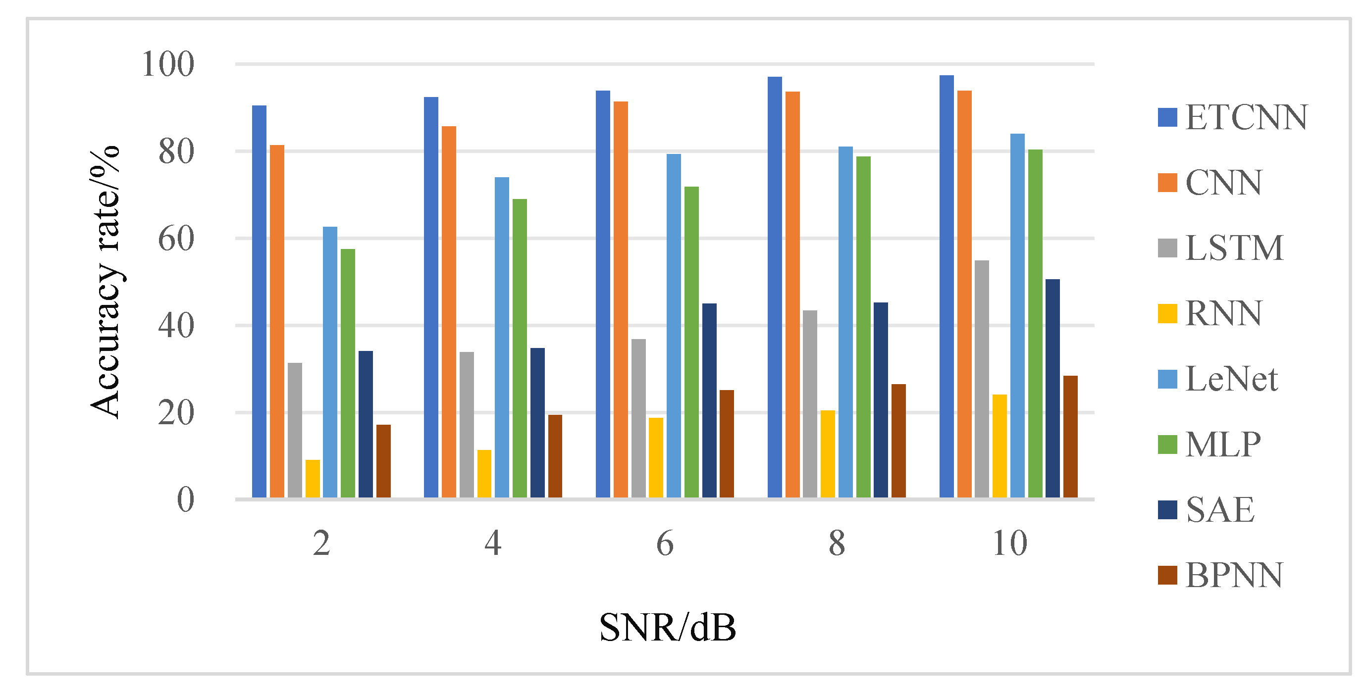
To analyze the robustness of SAWCA-Net, Gaussian white noise with different signal-to-noise ratios (SNRs) was added to the original vibration signal to simulate the signals collected in actual industrial practice. Samples containing 2 dB, 4 dB, 6 dB, 8 dB, and 10 dB Gaussian white noise were imported into the model for training and testing and compared with other deep learning models. The evaluation criteria mainly include diagnostic accuracy and F1 score, among which the F1 score reflects the performance of the evaluation method in each category. The final results are shown in Figure 8 and

Table 3. F1 scores (%) of eight models at various SNRs based on the CWRU dataset.

Model	2 dB	4 dB	6 dB	8 dB	10 dB
SAWCA-Net	90.37	92.31	93.97	96.92	97.31
CNN	80.99	85.44	91.25	93.61	93.87
LSTM	25.97	29.52	35.20	41.20	50.14
RNN	8.89	9.39	14.80	16.19	20.31
LeNet	62.35	73.95	79.25	80.92	83.93
MLP	57.94	69.22	72.07	79.28	80.56
SAE	38.94	39.52	42.67	45.82	51.27
BPNN	15.56	15.96	23.20	25.34	27.05

.

By observing Figure 8, it can be clearly seen that the method proposed in this paper is obviously superior to the other seven methods in fault diagnosis rate. With the increase of signal-to-noise ratio, the fault diagnosis rate of these eight methods also increases gradually. Figure 8 clearly shows that the accuracy of the proposed network is superior to the baselines under various SNR conditions. In addition, as can be seen from Table 3, the F1 score of the proposed method is in the front rank and performs best under various signal-to-noise ratios (SNRs). This result shows that this method can still maintain excellent fault diagnosis ability under the condition of high signal-to-noise ratio and maintain high diagnosis accuracy even under the condition of low signal-to-noise ratio and poor signal quality, showing excellent robustness and anti-interference.

4. Xi’an Jiaotong University Bearing Dataset

4.1. XJTU-SY Data Introduction

To further verify the fault identification performance of the proposed model, the XJTU-SY dataset collected by the Rolling Bearing Accelerated Life Test Bench of Xi’an Jiaotong University was introduced as the experimental data. This dataset was collected from the accelerated life test platform, and its structure is shown in Figure 9. The test platform is composed of an AC motor, a speed regulator, a transmission shaft, support bearings, test bearings, and a hydraulic loading system. It can simulate actual operating conditions by adjusting the speed and applying loads. In this experiment, LDK UER204 rolling bearings were selected as the test objects. The rotational speed was set between 2100 and 2250 rpm according to the load conditions. The hydraulic loading system applied radial loads of 12 kN, 11 kN, and 10 kN, respectively, under three working conditions. The sampling frequency of the vibration signal is 25.6 kHz, which is collected by the DT9837 portable dynamic data acquisition device. Two PCB 352C33 acceleration sensors are installed near the loading area of the bearing housing to measure the vibration signals in the horizontal and vertical directions, respectively.

Three working conditions were set up in the experiment. Each working condition included five sets of test bearings with different fault locations. A total of 15 sets of complete life cycle vibration data were obtained until the bearings failed. Vibration signals were continuously collected throughout the entire life cycle. With 1 s (25,600 points) as a sample length, 50% sliding window overlap was used for segmentation to enhance data utilization. In this paper, seven representative groups of data were selected for the experiment and divided into the training set and the test set in a ratio of 70%:30% to ensure that samples in the same time period do not appear simultaneously in the training set and the test set. The specific composition of the data and the fault labels are shown in

Table 4. Information Summary of XJTU SY Bearing Dataset.

Condition	Label	Dataset	Fault Type
1	0	Bearing 1_1	Outer Race
	1	Bearing 1_4	Cage
2	2	Bearing 2_1	Inner Race
	3	Bearing 2_2	Outer Race
	4	Bearing 2_2	Cage
3	5	Bearing 3_1	Outer Race
	6	Bearing 3_3	Inner Race

.

4.2. Comparative Experiment Based on the XJTU-SY Dataset

The method proposed in this paper is compared with the baselines. Each method is executed three times to ensure the reliability of the evaluation. The primary evaluation criteria are diagnostic accuracy and F1 score, where the F1 score reflects the balance between precision and recall for each category. The test results of the eight models are presented in Figure 10 and

Table 5. Experimental results of eight models based on the XJTU-SY dataset.

Model	Max Accuracy (%)	Min Accuracy (%)	Mean Accuracy (%)	Average F1 Score/%
SAWCA-Net	99.82	99.46	99.64 ± 0.15	99.64 ± 0.15
CNN	90.79	88.69	89.76 ± 0.86	89.69 ± 0.94
LSTM	41.13	39.89	40.62 ± 0.52	35.63 ± 0.49
RNN	17.10	15.66	16.23 ± 0.62	14.38 ± 1.33
LeNet	71.71	69.61	70.47 ± 0.90	70.69 ± 0.80
MLP	50.36	46.49	48.40 ± 1.58	48.47 ± 1.38
SAE	25.14	22.08	23.57 ± 1.25	23.40 ± 1.67
BPNN	21.85	19.71	20.81 ± 0.87	17.82 ± 0.74

.

It can be seen from the results in Figure 10 and Table 5 that the methods proposed in this question performed the best in terms of evaluation indicators and all have the lowest standard deviation. The superiority, robustness, and stability of the method proposed in this paper are thus proven. The diagnostic rates of LeNet, SAE, and BPNN did not exceed 30%, indicating the limitations of their feature extraction capabilities. In contrast, except for the method proposed in this paper, among the comparison methods, only the diagnosis rate of CNN reached 89.76%. Among them, the accuracy rate of classification diagnosis in this article increased particularly significantly. Specifically, compared with each comparison model, the average diagnosis rate of the method proposed in this paper increased by 9.95%, 64.01%, 85.26%, 28.95%, 51.17%, 76.24%, and 81.82%, respectively, which effectively verifies its outstanding performance improvement effect.

4.3. Signal-to-Noise Ratio Test

To analyze the robustness of the proposed network, Gaussian white noise with different signal-to-noise ratios (SNRs) was added to the original vibration signal to simulate the signals collected in actual industrial practice. Samples containing 2 dB, 4 dB, 6 dB, 8 dB, and 10 dB Gaussian white noise were imported into the proposed model for training and testing, and compared with other deep learning models. The evaluation criteria mainly include diagnostic accuracy and F1 score, among which the F1 score reflects the performance of the evaluation method in each category. The final results are shown in Figure 11 and

Table 6. F1 scores (%) of eight models at various SNRs.

Model	2 dB	4 dB	6 dB	8 dB	10 dB
SAWCA-Net	91.79	96.36	98.46	99.45	99.82
CNN	80.97	82.82	84.99	85.18	87.54
LSTM	14.45	16.43	18.59	23.13	39.84
RNN	10.70	14.53	14.55	14.76	15.69
LeNet	52.28	55.78	61.05	62.70	64.62
MLP	33.33	35.14	38.98	40.82	41.34
SAE	15.32	17.47	18.55	22.33	24.37
BPNN	14.86	15.75	16.04	17.04	17.36

.

It can be observed from the results that as the signal-to-noise ratio increases, the diagnostic accuracy and F1 scores obtained by the eight models also increase. When the SNR reaches 12 dB, the diagnostic accuracy for noisy signals almost reaches the judgment accuracy for noise-free signals. However, in terms of the overall diagnostic accuracy rate, under various SNRs, the fault diagnosis rate and F1 score of the proposed network are higher than those of other models. This result indicates that model can maintain high fault diagnosis performance under different signal-to-noise ratio conditions. Even in the case of high noise, SAWCA-NET can still effectively capture key features and improve the robustness of fault diagnosis.

5. PRONOSTIA Bearing Failure Dataset

5.1. PRONOSTIA Data Introduction

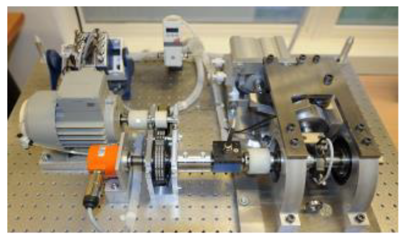
In order to further verify the fault diagnosis ability of the proposed SAWCA-NET model in a real industrial environment, this paper introduces the PRONOSTIA bearing failure dataset released by the FEMTO-ST Institute in France for experimental evaluation. This dataset systematically simulates typical industrial working conditions, including constant and adjustable loads, high-speed rotation, temperature control, etc., by constructing a highly controllable and repeatable bearing accelerated degradation experimental platform. The experimental platform is shown in Figure 12. PRONOSTIA data are characterized by authenticity, complexity, and engineering representativeness and can more comprehensively reflect the dynamic degradation process of equipment operation in industrial scenarios.

This dataset collects the operating status data of bearings with high temporal resolution. Specifically, it collects vibration signals every 10 s, with each sampling lasting for 1 s and with a sampling frequency of 25.6 kHz, forming a complete degradation process covering the bearings from the initial normal state to the final failure stage. The types of faults included are quite diverse, covering a variety of typical bearing failure modes such as inner ring spalling, outer ring spalling, rolling element fatigue, and natural compound faults. It is worth noting that some of the degraded bearing samples in the PRONOSTIA platform have multiple types of defects simultaneously (such as compound damage to components like balls, rings, and cages), further increasing the complexity of faults and diagnostic challenges in the data, thereby enhancing the authenticity and practical value of this dataset for evaluating the performance of model detection.

5.2. Comparative Test Results Analysis

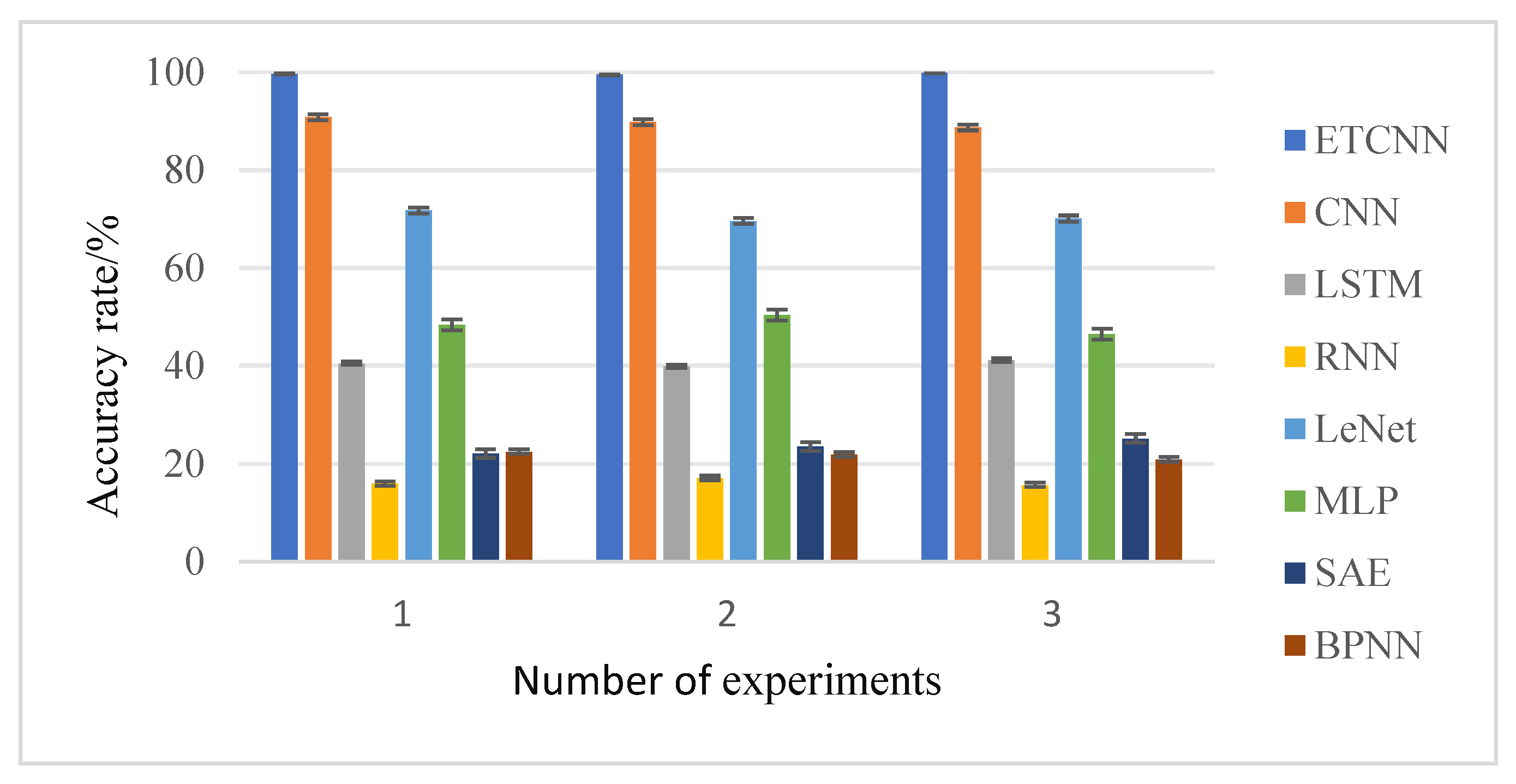
To verify the performance of the proposed network, this paper systematically compares it with the baselines on the PRONOSTIA dataset. Each model was run three times under the same training–test division, and the highest accuracy rate, the lowest accuracy rate, the average accuracy rate, and its standard deviation were recorded. The test results of the eight models are shown in Figure 13 and

Table 7. Experimental results of eight models based on the PRONOSTIA dataset.

Model	Max Accuracy (%)	Min Accuracy (%)	Mean Accuracy (%)
SAWCA-Net	98.10	97.02	97.58 ± 0.31
CNN	88.75	85.62	87.18 ± 1.56
LSTM	36.42	33.95	35.10 ± 0.92
RNN	17.10	15.66	16.23 ± 0.62
LeNet	71.71	69.61	70.47 ± 0.90
MLP	50.36	46.49	48.40 ± 1.58
SAE	25.14	22.08	23.57 ± 1.25
BPNN	21.85	19.71	20.81 ± 0.87

.

It can be seen from the experimental results that the fault diagnosis accuracy and stability of the proposed network on the PRONOSTIA dataset are significantly better than those of other mainstream models, demonstrating strong comprehensive performance. In the three independent experiments, its average accuracy rate reached 98.85% ± 0.25; this was not only the highest among all the comparison models but also the smallest standard deviation, demonstrating good robustness and reliability. In contrast, the average accuracy rate of CNN is 89.63%, while LSTM and RNN perform poorly in complex working conditions due to their difficulty in effectively modeling non-stationary weak fault features, with average accuracy rates of only 40.62% and 16.23%, respectively. Compared with the baselines, the accuracy rates of the proposed network increased by 3.02%, 44.22%, 71.73%, 7.78%, 14.26%, 48.30%, and 62.79%, respectively. This comprehensively verifies the proposed network’s advantages in feature extraction, pattern recognition, and adaptability to complex working conditions and its high practical engineering value.

5.3. Signal-to-Noise Ratio Test on PRONOSTIA

To further evaluate the robustness of the proposed network under noise interference, in this paper, Gaussian white noise with different SNR levels (2 dB, 4 dB, 6 dB, 8 dB, and 10 dB respectively) is introduced into the original vibration signal of PRONOSTIA, and its performance is compared with that of other deep learning models under the same settings through experiments. The experimental evaluation indicators include diagnostic accuracy and F1 score. The results are shown in Figure 14 and

Table 8. F1 scores (%) of eight models at various SNRs based on the PRONOSTIA dataset.

Model	2 dB	4 dB	6 dB	8 dB	10 dB
SAWCA-Net	87.25	91.02	96.21	97.85	98.15
CNN	76.53	78.41	81.65	83.20	85.10
LSTM	11.84	14.02	16.58	20.13	35.10
RNN	9.41	13.10	13.67	13.82	15.06
LeNet	48.12	51.95	57.34	59.26	62.10
MLP	31.76	33.82	37.25	39.43	40.12
SAE	14.05	16.01	17.62	21.16	23.78
BPNN	13.52	14.91	15.80	16.53	16.87

.

It can be observed from the results that under different SNR conditions, this proposed network performs the best in fault identification. Even in the case of relatively high noise (such as 2 dB), its F1 score reached 89.36%, significantly higher than models like CNN (78.92%), LeNet (50.15%), and MLP (31.76%). At 10 dB, the F1 score even reached 99.16%, approaching its performance under noise-free conditions. In contrast, time series models such as LSTM and RNN perform poorly at low signal-to-noise ratios. Their F1 scores are only 13.07% and 9.41% at 2 dB, and even at 10 dB, they do not exceed 40% and 16%. This indicates that they have difficulty effectively identifying weak fault features in noisy environments. Overall, the proposed network can maintain a high diagnostic accuracy at different noise levels, demonstrating good anti-noise ability and practical application value.

6. Experimental Environment, Model Efficiency, and Generalization Analysis

6.1. Experimental Environment and Training Configuration

All model training and testing in this article were completed on a single workstation configured with an Intel^® Core™ i7-8700 CPU at 3.20 GHz, 32 GB of memory, and an NVIDIA^® RTX 3080 GP and run on the Windows 11 operating system. The software environment is Python 3.9, using the PyTorch 1.12 deep learning framework and enabling CUDA 11.6 acceleration.

To simulate and evaluate the performance of SAWCA-Net in typical rolling bearing monitoring scenarios under controllable conditions, the processing methods of various public datasets in this paper simulate the input/output processes of actual industrial condition monitoring systems. The data acquisition device includes the following:

• CWRU platform: SKF 6205-2RS bearings are installed on the motor drive test bench. PCB 352C33 acceleration sensors are installed at the drive end/fan end, with a sampling frequency of 12–48 kHz;
• XJTU-SY platform: The LDK UER204 bearing is installed on the accelerated life test bench. PCB 352C33 acceleration sensors are arranged in the horizontal and vertical directions, respectively, with a sampling frequency of 25.6 kHz;
• PRONOSTIA platform: Industrial-grade bearings operate under constant load and variable load conditions, collecting vibration signals of a length of 1 s every 10 s at a sampling frequency of 25.6 kHz.

All vibration signals are preprocessed and input into the SAWCA-Net inference module in a manner consistent with online monitoring, thereby reproducing the data flow in the actual condition monitoring system.

To comprehensively evaluate the practical application potential of the proposed model, this paper compares it with the classic convolutional neural network ResNet18 in terms of model parameter scale, computational cost (FLOP), and single-sample inference time. The results show that the parameter quantity of this model is approximately 1.2 million, the FLOP is approximately 90 million times, and the single-sample inference time is approximately 5.6 milliseconds. The parameter count of ResNet18 is approximately 11.7 million, its FLOP is about 180 million operations, and its inference time is approximately 9.8 milliseconds. In contrast, the proposed model, while maintaining a high diagnostic accuracy rate, significantly reduces model complexity and computational burden, enhances real-time reasoning performance, and possesses stronger adaptability to industrial sites and engineering application value.

6.2. Cross-Validation Results and Generalization Analysis

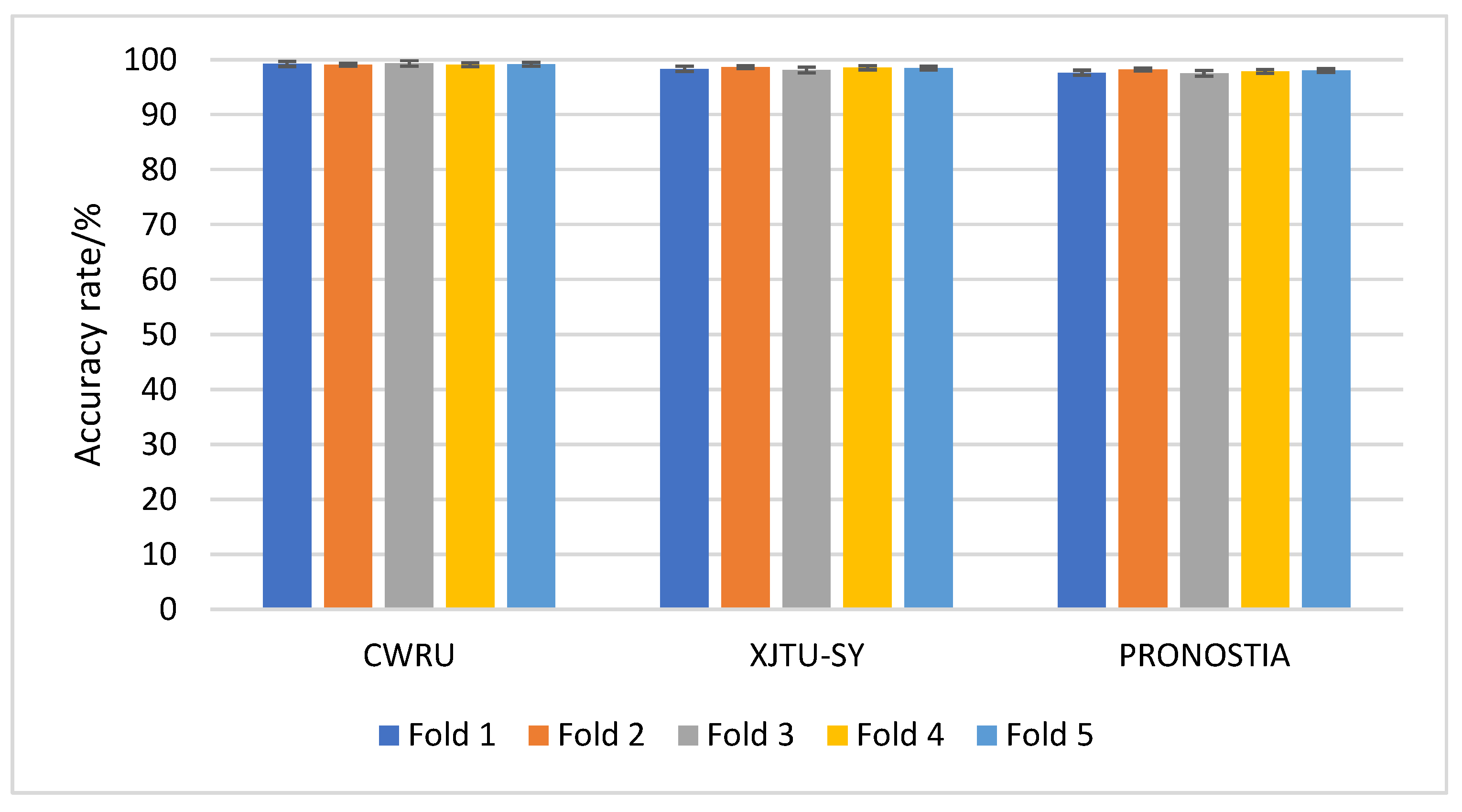
To comprehensively evaluate the generalization ability of the proposed model, this paper conducts hierarchical 5-fold cross-validation experiments on three public bearing fault datasets, namely CWRU, XJTU-SY, and PRONOSTIA. During the division process, we ensured that the category and working condition distribution of each fold were consistent, strictly avoiding the same test bearing or samples from the same time series appearing simultaneously in the training set and the validation set to prevent information leakage. Regarding hyperparameter adjustment, each training subset was further adopted to select the optimal hyperparameters, thereby ensuring the objectivity and robustness of the evaluation results. Thus, Figure 15 and

Table 9. Cross-validation results of the three datasets.

Fold	CWRU	XJTU-SY	PRONOSTIA
Fold 1	99.24	98.32	97.62
Fold 2	99.08	98.68	98.21
Fold 3	99.34	98.12	97.52
Fold 4	99.10	98.53	97.88
Fold 5	99.15	98.45	98.00
Mean ± Std	99.18 ± 0.12	98.42 ± 0.21	97.84 ± 0.28

are presented.

As can be seen from Table 9, the performance of the proposed model on the three datasets is at a relatively high level with minimal fluctuations: among them, the average accuracy of the CWRU dataset is 99.18%, and the standard deviation is only ±0.12%, demonstrating the high stability of the results under different data divisions. The average accuracy rate of the XJTU-SY dataset is 98.42% ± 0.21%, and it also shows good robustness. The average accuracy rate of the PRONOSTIA dataset is 97.84% ± 0.28%. Although it is slightly lower among the three, it still maintains a relatively high classification accuracy. The standard deviations of all datasets were controlled within ±0.3%, indicating that the performance fluctuations of the model at different intervals were extremely small, and it had good stability and generalization ability.

7. Conclusions and Prospects

7.1. Conclusions

Aiming at the problem of difficult fault identification of rolling bearings in a background of strong noise, this paper proposes a deep neural network model, namely SAWCA-Net, that integrates the spectrum-adaptive wide convolution and the dynamic time–channel attention mechanism. This method, by integrating time-domain and frequency-domain feature information, enables the model’s receptive field and sampling position to be dynamically adjusted according to the input, thereby effectively enhancing the modeling ability and anti-noise performance for non-stationary periodic signals. Meanwhile, the introduced interactive attention mechanism strengthens the key feature extraction process, which helps to enhance the perception ability of weak fault signals and suppress redundant interference.

The experimental results conducted on the PRONOSTIA bearing degradation dataset of CWRU, the Experimental Platform of XJTU-SY, and the FEMTO-ST Institute show the following:

(1) The maximum classification accuracy rates of the proposed network on the CWRU and XJTU-SY datasets were 99.15% and 99.64%, respectively. On the PRONOSTIA dataset, the three experiments were all stable at above 98.6%, and the average accuracy rate reached 98.85%, which was significantly better than the traditional model. This fully verifies its excellent fault identification ability and generalization performance.

(2) The feature space output by the model was analyzed through t-SNE visualization. It was found that the features extracted by this proposed model had clear boundaries between categories and good intra-class aggregation, indicating that the model had a strong feature expression ability.

(3) After adding Gaussian white noise for testing under different SNR conditions, the proposed network still maintained high accuracy and F1 scores. Even under extreme noise interference of 2 dB, it could achieve an F1 score of 89.36%, far exceeding other comparison models, demonstrating excellent noise immunity and robustness.

Although good results have been achieved, there are still two deficiencies: First, this study only evaluated a single fault type, and the diagnostic ability for compound faults and progressive faults still needs further verification; second, the adaptability of the model to different types of bearings, working conditions, and equipment still needs to be confirmed through more extensive tests.

7.2. Outlook

Although SAWCA-Net demonstrated strong stability and adaptability in multiple typical datasets and complex working conditions, there are still several directions worthy of further exploration to promote its in-depth application in actual industrial scenarios:

(1) Model simplification and deployment optimization: Industrial sites typically have high requirements for computing resources and response speed. In the future, attempts can be made to reduce the computing overhead of the network through methods such as model compression, parameter pruning, and quantization, making it more suitable for deployment and operation on edge computing devices or embedded terminals.

(2) Multi-source information fusion modeling: Relying solely on vibration signals may make it difficult to comprehensively reflect the equipment status. If multiple sensor data, such as temperature, acoustic emission, current, and voltage, can be introduced for fusion analysis, it is expected to enhance the perception ability of the fault development process and provide a richer information basis for diagnosis and early warning.

(3) Enhanced adaptability and online updates: During long-term operation, the status and working conditions of the equipment may constantly change. To address this dynamic nature, mechanisms such as incremental learning, transfer learning, or federated learning can be introduced to endow the model with continuous learning capabilities and enhance its adaptability and reliability in real-world environments.

(4) Planned real-motor deployment: We will pilot the proposed method on industrial induction motors driving fans and pumps in a plant-level setting. The deployment will fuse motor-housing vibration signals (tri-axial accelerometers) with motor current and phase voltage measurements for complementary sensing, using sampling rates of 12–25.6 kHz for vibration and 10–20 kHz for electrical signals. The model will be deployed on an edge device (industrial PC or NVIDIA Jetson), targeting inference latency of less than 10 ms per analysis window. Effectiveness will be evaluated in terms of accuracy, F1-score, and AUC as well as sensitivity, specificity, false-alarm rate (<1%/day), and time-to-detect (TTD) relative to maintenance logs. To enhance cross-motor generalization, domain adaptation strategies will be applied, and periodic online updates will be scheduled to accommodate changes in operating conditions. Subject to site policy, a de-identified subset of the real-motor data and the evaluation scripts will be released to facilitate reproducibility.

7.3. Method Comparison and Summary

It is worth mentioning that in recent studies, Zhu et al. [24] proposed a network model based on multi-scale residual structure and hybrid attention mechanism, achieving an accuracy rate of 99.7% on the Paderborn bearing dataset, demonstrating its outstanding performance under ideal operating conditions. However, the dataset relied upon by this research has relatively single operating conditions and lacks verification in a complex and real industrial context.

In contrast, the SAWCA-Net model proposed in this paper demonstrates stable and outstanding performance on multiple public datasets (CWRU, XJTU-SY, and PRONOSTIA) under various working conditions, multiple types of faults, and different noise levels, showing stronger robustness and wide adaptability. In terms of structural design, the proposed network integrates a spectral-driven dynamic convolution mechanism and a time–channel interactive attention module, which can capture weak periodic fault features more effectively and is suitable for rolling bearing diagnosis tasks in complex environments.

In summary, although the highest accuracy rate in some ideal datasets is slightly lower than that of some of the latest models, the proposed network has more advantages in modeling concepts, noise resistance capabilities, and practical applicability, providing a robust and effective solution for intelligent diagnosis of bearing faults in the engineering field.

References

1. Zhan, L.; Li, Z.; Chi, J.; Zhuo, S.; Li, C. Fault size estimation of rolling bearing based on weak magnetic detection. Mech. Syst. Signal Process. 2023, 192, 110230. [Google Scholar] [CrossRef]
2. Jiang, L.; Shi, C.; Sheng, H.; Li, X.; Yang, T. Lightweight CNN architecture design for rolling bearing fault diagnosis. Meas. Sci. Technol. 2024, 35, 126142. [Google Scholar] [CrossRef]
3. Qin, Y.; Yang, R.; Shi, H.; He, B.; Mao, Y. Adaptive Fast Chirplet Transform and Its Application into Rolling Bearing Fault Diagnosis Under Time-Varying Speed Condition. IEEE Trans. Instrum. Meas. 2023, 72, 3519212. [Google Scholar] [CrossRef]
4. Shao, Z.; Zhu, Y.; Zhang, P.; Cao, Y.; Wang, B.; Xu, Z.; Liu, H.; Gu, X.; Liu, H.; Li, D.; et al. Effect of primary carbides on rolling contact fatigue behaviors of M50 bearing steel. Int. J. Fatigue 2024, 179, 108054. [Google Scholar] [CrossRef]
5. Kibrete, F.; Woldemichael, D.E.; Gebremedhen, H.S. Multi-Sensor data fusion in intelligent fault diagnosis of rotating machines: A comprehensive review. Measurement 2024, 232, 114658. [Google Scholar] [CrossRef]
6. Xiao, M.; Wang, Z.; Zhao, Y.; Geng, G.; Dustdar, S.; Donta, P.K.; Ji, G. A new fault feature extraction method of rolling bearings based on the improved self-selection ICEEMDAN-permutation entropy. ISA Trans. 2023, 143, 536–547. [Google Scholar] [CrossRef] [PubMed]
7. Chaleshtori, A.E.; Aghaie, A. A novel bearing fault diagnosis approach using the Gaussian mixture model and the weighted principal component analysis. Reliab. Eng. Syst. Saf. 2024, 242, 109720. [Google Scholar] [CrossRef]
8. Fu, L.; Wang, S.; Chen, R.; Ma, Z.; Ma, J.; Yao, B.; Xu, F. Intelligent fault diagnosis of rolling bearings based on an improved empirical wavelet transform and resnet under variable conditions. IEEE Sens. J. 2023, 23, 29097–29108. [Google Scholar] [CrossRef]
9. Chen, S.; Zheng, X. A bearing fault diagnosis method with improved symplectic geometry mode decomposition and feature selection. Meas. Sci. Technol. 2024, 35, 046111. [Google Scholar] [CrossRef]
10. Jamil, M.A.; Khanam, S. Influence of one-way ANOVA and Kruskal–Wallis based feature ranking on the performance of ML classifiers for bearing fault diagnosis. J. Vib. Eng. Technol. 2024, 12, 3101–3132. [Google Scholar] [CrossRef]
11. Fu, Y.; Zhou, Q.; Tang, H. A Dual-Level Intelligent Architecture-Based Method for Coupling Fault Diagnosis of Temperature Sensors in Traction Converters. Machines 2025, 13, 590. [Google Scholar] [CrossRef]
12. Huang, Z.; Zhao, X. A novel multi-scale competitive network for fault diagnosis in rotating machinery. Eng. Appl. Artif. Intell. 2024, 128, 107441. [Google Scholar] [CrossRef]
13. Jia, B.; Liang, G.; Huang, Z.; Song, X.; Liao, Z. Rotating Machinery Structural Faults Feature Enhancement and Diagnosis Based on Multi-Sensor Information Fusion. Machines 2025, 13, 553. [Google Scholar] [CrossRef]
14. Gao, R.; Zhu, J.; Wu, Y.; Xiao, K.; Shen, Y. Research on Bearing Fault Diagnosis Method Based on MESO-TCN. Machines 2025, 13, 558. [Google Scholar] [CrossRef]
15. Wang, Z.; Luo, Q.; Chen, H.; Zhao, J.; Yao, L.; Zhang, J.; Chu, F. A high-accuracy intelligent fault diagnosis method for aero-engine bearings with limited samples. Comput. Ind. 2024, 159, 104099. [Google Scholar] [CrossRef]
16. Han, K.; Wang, W.; Guo, J. Research on a Bearing Fault Diagnosis Method Based on a CNN-LSTM-GRU Model. Machines 2024, 12, 927. [Google Scholar] [CrossRef]
17. Jiang, W.; Qi, Z.; Jiang, A.; Chang, S.; Xia, X. Lightweight network bearing intelligent fault diagnosis based on VMD-FK-ShuffleNetV2. Machines 2024, 12, 608. [Google Scholar] [CrossRef]
18. Misbah, I.; Lee, C.K.M.; Keung, K.L. Fault diagnosis in rotating machines based on transfer learning: Literature review. Knowl. Based Syst. 2024, 283, 111158. [Google Scholar] [CrossRef]
19. Oppenheim, A.V.; Schafer, R.W. Discrete-Time Signal Processing, 3rd ed.; Prentice Hall: Upper Saddle River, NJ, USA, 1999. [Google Scholar]
20. Smith, S.W. The Scientist and Engineer’s Guide to Digital Signal Processing; California Technical Publishing: San Diego, CA, USA, 2003. [Google Scholar]
21. Dai, J.; Qi, H.; Xiong, Y.; Li, Y.; Zhang, G. Deformable Convolutional Networks. In Proceedings of the IEEE International Conference on Computer Vision (ICCV), Venice, Italy, 22–29 October 2017; pp. 764–773. [Google Scholar]
22. Hu, J.; Shen, L.; Sun, G. Squeeze-and-Excitation Networks. In Proceedings of the IEEE/CVF Conference on Computer Vision and Pattern Recognition (CVPR), Salt Lake City, UT, USA, 18–23 June 2018; pp. 7132–7141. [Google Scholar]
23. Woo, S.; Park, J.; Lee, J.-Y.; Kweon, I.S. CBAM: Convolutional Block Attention Module. In Proceedings of the European Conference on Computer Vision (ECCV), Munich, Germany, 8–14 September 2018; pp. 3–19. [Google Scholar]
24. Zhu, Y.; Chen, W.; Yan, S.; Zhang, J.; Zhu, C.; Wang, F.; Chen, Q. Multi-Scale Residual Convolutional Neural Network with Hybrid Attention for Bearing Fault Detection. Machines 2025, 13, 413. [Google Scholar] [CrossRef]
Figure 1. SAWCA-Net structural model.
Machines 13 00795 g001
Figure 2. Structure diagram of S-AWKC.
Machines 13 00795 g002
Figure 3. DI-TCAM Network Structure Diagram.
Machines 13 00795 g003
Figure 4. SAWCA-Net diagnostic process.
Machines 13 00795 g004
Figure 5. CWRU Bearing Test Rig.
Machines 13 00795 g005
Figure 6. Accuracy of each method based on the CWRU dataset.
Machines 13 00795 g006
Figure 7. Visualization results: (a) t-SNE visualization; (b) confusion matrix.
Machines 13 00795 g007
Figure 8. Diagnostic accuracy of eight models under various SNRs based on the CWRU dataset.
Machines 13 00795 g008
Figure 9. XJTU-SY bearing test bench.
Machines 13 00795 g009
Figure 10. Accuracy of each method based on the XJTU-SY dataset.
Machines 13 00795 g010
Figure 11. Diagnostic accuracy of eight models under various SNRs.
Machines 13 00795 g011
Figure 12. PRONOSTIA bearing test bench.
Machines 13 00795 g012
Figure 13. Accuracy of each method based on the PRONOSTIA dataset.
Machines 13 00795 g013
Figure 14. Diagnostic accuracy of eight models under various SNRs based on the PRONOSTIA dataset.
Machines 13 00795 g014
Figure 15. The diagnostic accuracy of cross-validation among the three datasets.
Machines 13 00795 g015