Analytical Approach to Estimate Temperature Variations in Passively Cooled Train Inverters

Abstract

The advent of silicon carbide (SiC) semiconductors in electric traction enables several benefits, including the shift to passive cooling. However, it requires a conjugate heat transfer analysis to understand the temperature distribution and variation. While steady-state solutions exist, transient conditions in rail vehicles remain challenging. This paper develops two analytical models to predict temperature distribution and variation, validated against numerical simulations. An electric motor model estimates power losses in the converter, defining heat dissipation. The complete model is tested under realistic drive cycles, linking operational conditions to power losses and free flow speed. The results show the model effectively captures temperature variations, with higher losses during acceleration and larger temperature surges of around 70 K at lower speeds. Furthermore, the temperature at the junction was observed to be 20 K higher than at the base position and to exceed 420 K at a more downstream location. Thus, the proposed method captures the temperature variations considering different physical effects with reasonable accuracy and significantly faster computation times than transient numerical simulations.

1. Introduction

With the recent developments on silicon carbide (SiC) power electronics, new opportunities have opened for optimizing rail vehicle traction system efficiency [1]. Its main benefits over silicon-based components are a wider range of tolerable temperatures and higher switching frequencies. For electronic converters on trains, this translates into a reduction of nearly 30% in weight and 50% in volume [2] and reduced energy losses due to current switching, allowing more efficient motor driving. It has already been successfully tested in Japanese high-speed trains [3,4], where the motor and the power electronics box have been significantly reduced in size.

For power electronics, the use of SiC also enables simplifying the cooling system, reducing even more the size, weight, and complexity of these components. Instead of active cooling with a liquid coolant [5] or forced-air cooling with fans [6], electronics can be cooled down passively using the convection airflow below the moving train, as demonstrated on the Shinkansen [3]. This means that effective cooling is provided without the need for fans, etc., and so such a component could be omitted along with their associated energy and volume demands. There are, however, system-dependent challenges as the cooling effect is directly dependent on the motion of the train. So, for lower-speed trains like metros, the potential cooling will be reduced. The recent success of a pilot test in the Stockholm metro [2] encourages the research on cooling modeling for this specific application.

From an operational perspective, there is a certain lack of alignment between the traction power and speed of the vehicle for different operational scenarios. Higher speeds will enhance cooling, while high-power peaks and the subsequent high energy dissipation in the converters are arguably highest during the acceleration phase from standstill, where the speed is near-zero. The present paper investigates the temperature variations in the electronic system during train operation. Both traction power and train speed impact the temperature evolution on the converters: when the motor operates at higher power, the electronic system heats up more, whilst for larger speeds, the cooling is more efficient. A balance between the source of heating and the dissipation must be ensured at all times in order to avoid any overheating, and the transitions make it a non-steady-state problem.

Numerically, simulating this interaction is very challenging as it couples two different types of problems: the conduction of the heat generated by the drive system and the convective cooling of the air flowing past the electronic system. Computational fluid dynamics (CFD) simulations are very costly for that kind of coupling, and simple models are sought to derive new designs. There are also a limited amount of articles in the literature that deal with the modeling of this coupling.

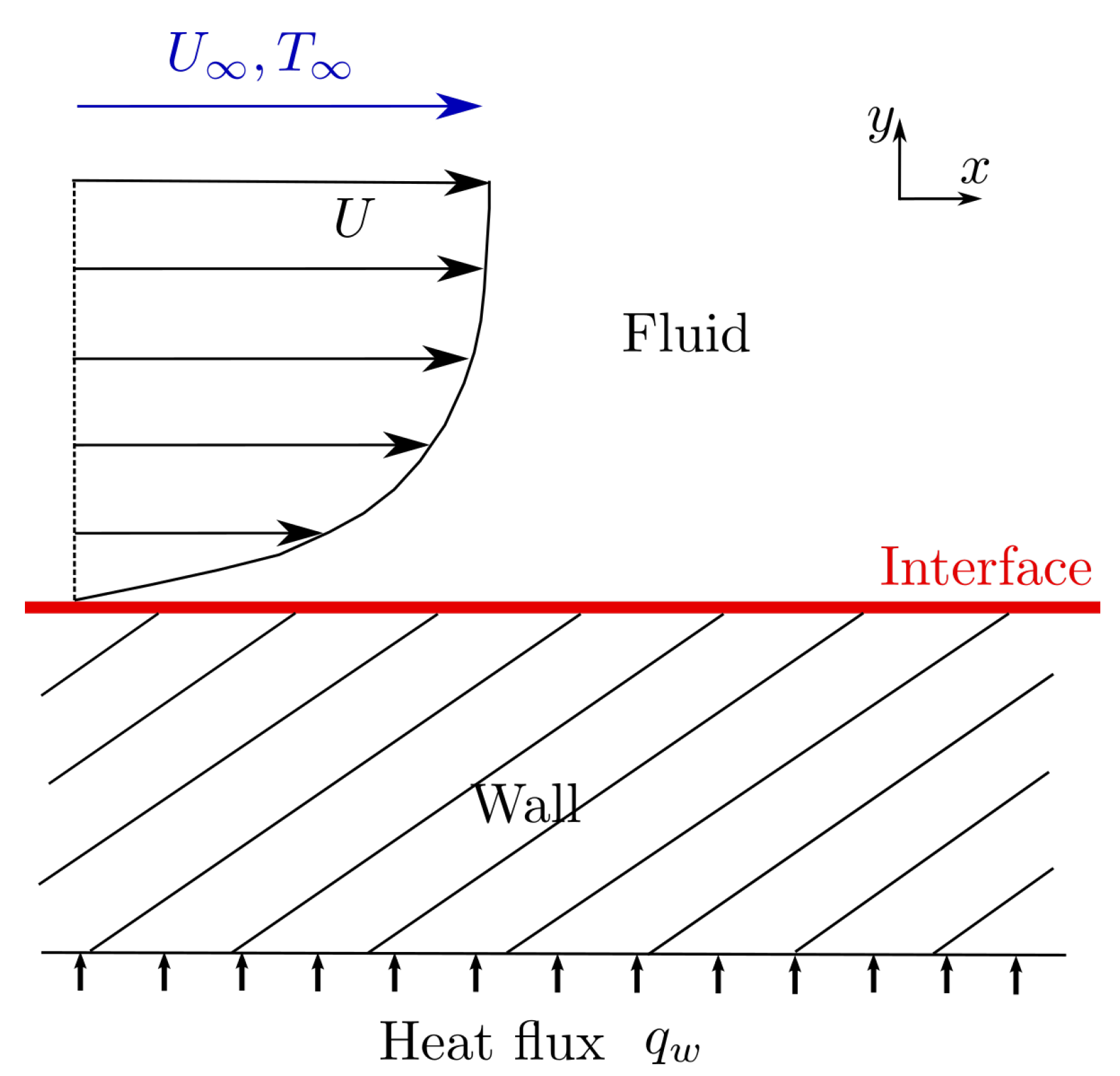
These types of problems are known as conjugate heat transfer (CHT) problems, which are complex fluid mechanics problems that study the conduction in a solid interacting with the convection of the fluid flowing past the solid. Figure 1 illustrates a classical CHT problem, the interaction between the conductive flow through the slab generated by the heat flux $q_w$ from below and the airflow. Steady-state predictions can reasonably be achieved with a good level of accuracy [7]. However, transient developments of the temperature at the interface between the solid and the fluid are usually much harder to estimate. This is crucial when applied to trains power electronics: large temperature peaks may damage the converters and potentially degrade their functioning in operation.

Due to the difference in time scales between conduction and convection processes, computational fluid dynamics (CFD) simulations are numerically challenging [8]. The required fluid mesh needs to be refined enough to accurately capture the fluid dynamics, but the physical simulated time for the coupled solid/fluid system is much larger than the advection time. Because of the mesh refinement, some elements are very small and need to be numerically solved with a small time-step in the CFD simulation. This means that with a small time-step and a long physical simulated time, the simulation needs many iterations and a long time to converge.

The major difficulty in classical CHT problem is to capture the unsteadiness of the temperature subsequent to the variations of either or both the speed and the heat flux over time [9].

Therefore, in this article, the objective is to develop a method that captures the temperature variations at the surface of the electronic inverters by considering as many physical effects as possible with a much lower computational cost than a CFD simulation. To demonstrate the developed method, a simplistic inverter model representative of a metro train inverter is used in combination with an operational drive cycle, which provides information on track geometry, speed, the number of traction motors, and traction power.

By utilizing such simplified models, the analysis can be focused on the region where one of the most critical thermal exchanges in the inverter occur, thereby allowing the essential physics of the problem to be captured while keeping the computational complexity manageable.

The method proposed in this article to estimate the temperature evolution at the surface of electronic inverters addresses two key aspects:

• The speed of the flow cooling the inverter varies over time like the train speed in real conditions;
• The power loss and the heat generated by the converters are calculated simultaneously from the variations of the traction power of the motor.

An element of focus in the study is the integration of electronic and aerodynamic factors influencing the thermal behavior of the converters coupled via the operational drive cycle, thus highlighting the multidisciplinary aspect of this study. Initially, the process involved in developing a simplified passive convection cooling model is explained. Subsequently, the converter power losses are derived, and the electric motor operation is described. Finally, the complete model is coupled and tested with speed and traction power derived from a realistic operational drive cycle of a metro train to predict the temperature variations over the entire drive cycle.

2. Modeling of Passive Cooling

The idea of passively cooling down the electronics on the train is to make use of the airflow around the cars. The heat sink is designed to maximize the thermal exchange with the air flowing in between the fins so that the power loss from the electronics can be dissipated efficiently. This is where the coupling between the conduction of the heat generated by the converters and the cooling effect due to the convection takes place.

2.1. Analytical Modeling of Conjugate Heat Transfer

In order to address the computational challenges of conjugate heat transfer problems, analytical methods are hereby investigated as an efficient way of estimating the temperature at the interface. Before developing the analytical method, it is recalled that the variations of the train speed are modeled by the variations of the freestream velocity $U_{\infty }$, the velocity developed far from the wall of the modeled converter, over which the velocity reaches zero. This means that the in-between boundary layer must be modeled correctly to be representative of the heat exchange between the flow and the wall.

Such models seek to capture as many effects as possible of the physics at much lower cost than a CFD simulation that solves the Navier–Stokes equations.

2.1.1. Boundary Layer Thickness Estimate

Several methods exist in the literature to analytically predict the shape of the boundary layer on the speed and the temperature. Here, the principle of the modeling is based on Karman–Pohlhausen’s method (KPM) [10], which considers a steady parallel laminar and incompressible flow past a zero-thickness semi-infinite flat plate. The values characterizing the incident flow are its temperature $T_{\infty }$ and velocity $U_{\infty }$. Karman–Pohlhausen’s method is based on the approximation of the boundary layers by polynomials. It leads to quite good estimates of the boundary layer growth streamwise.

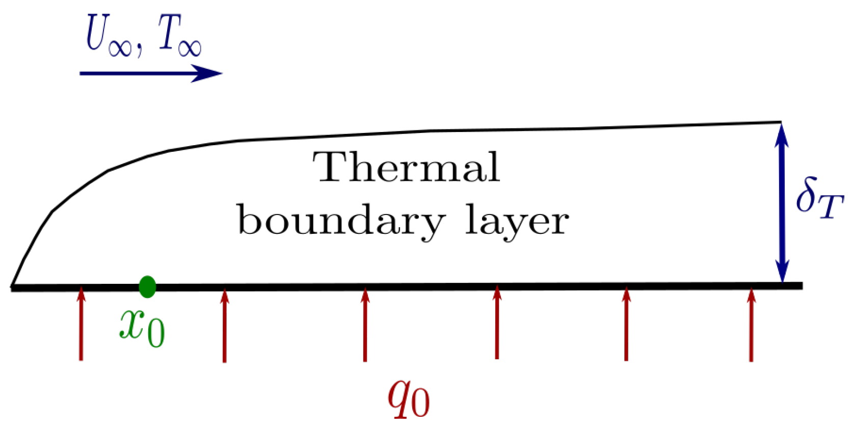
The problem studied is illustrated in Figure 2. The flat plate is submitted to a heat supply $q_0$. The objective is to estimate the temperature at the interface $T_w$, at any position $x_0$ along the flat plate, in the stream direction. The application of KPM is thoroughly described by Lachi et al. [11], and the method is used in the same way in the present paper. By approximating the velocity and the temperature by polynomials, the energy equation in the Navier–Stokes equations can be solved:

$${\displaystyle \frac{\mathsf{\partial }}{\mathsf{\partial }t}}{\int }_0^{{\delta }_t}\theta \mathrm{d}y+{\displaystyle \frac{\mathsf{\partial }}{\mathsf{\partial }x}}{\int }_0^{{\delta }_t}U\theta \mathrm{d}y=-{\alpha }_{\mathrm{air}}{\left.{\displaystyle \frac{\mathsf{\partial }\theta }{\mathsf{\partial }y}}\right|}_{y=0}$$

(1)

$\theta \left(y\right)$ represents the temperature difference $T\left(y\right)-T_{\infty }$, and the interest specifically lies in what happens for $y=0$. The temperature and the velocity are approximated by fourth-order polynomials here and the boundary conditions on the velocity and the temperature enable to calculate the sets of coefficients of the polynomials. This leads to an estimate of the boundary layer thicknesses $\delta$ and ${\delta }_t$, enabling to solve Equation (1) numerically.

Figure 2. Sketch of the flat plate configuration.

Figure 2. Sketch of the flat plate configuration.

Indeed, the equation can be rewritten by substitution of ${\delta }_t$, U, and $\theta$ as a partial differential equation, as follows:

$$a_0+a_1{\theta }_w+a_2{\theta }_w^2+a_3{\theta }_w^3+a_4{\theta }_w^4+a_5{\theta }_w^5+a_6{\theta }_w^6=0$$

(2)

The coefficients a are detailed in Lachi’s paper [11]. Some of them depend on x and t and feature a partial derivative of the temperature difference. The equation is solved by using a first-order upwind scheme using the same discretization of time and space as that used by Lachi et al.

Starting at $x=0$ and $t=0$, the polynomial equation is solved numerically with numpy.roots in Python 3.10, and the only positive real root is selected among the six complex roots. Iteratively, the temperature difference ${\theta }_w$ distribution in time and space can be reconstructed.

2.1.2. Thermal Impedances

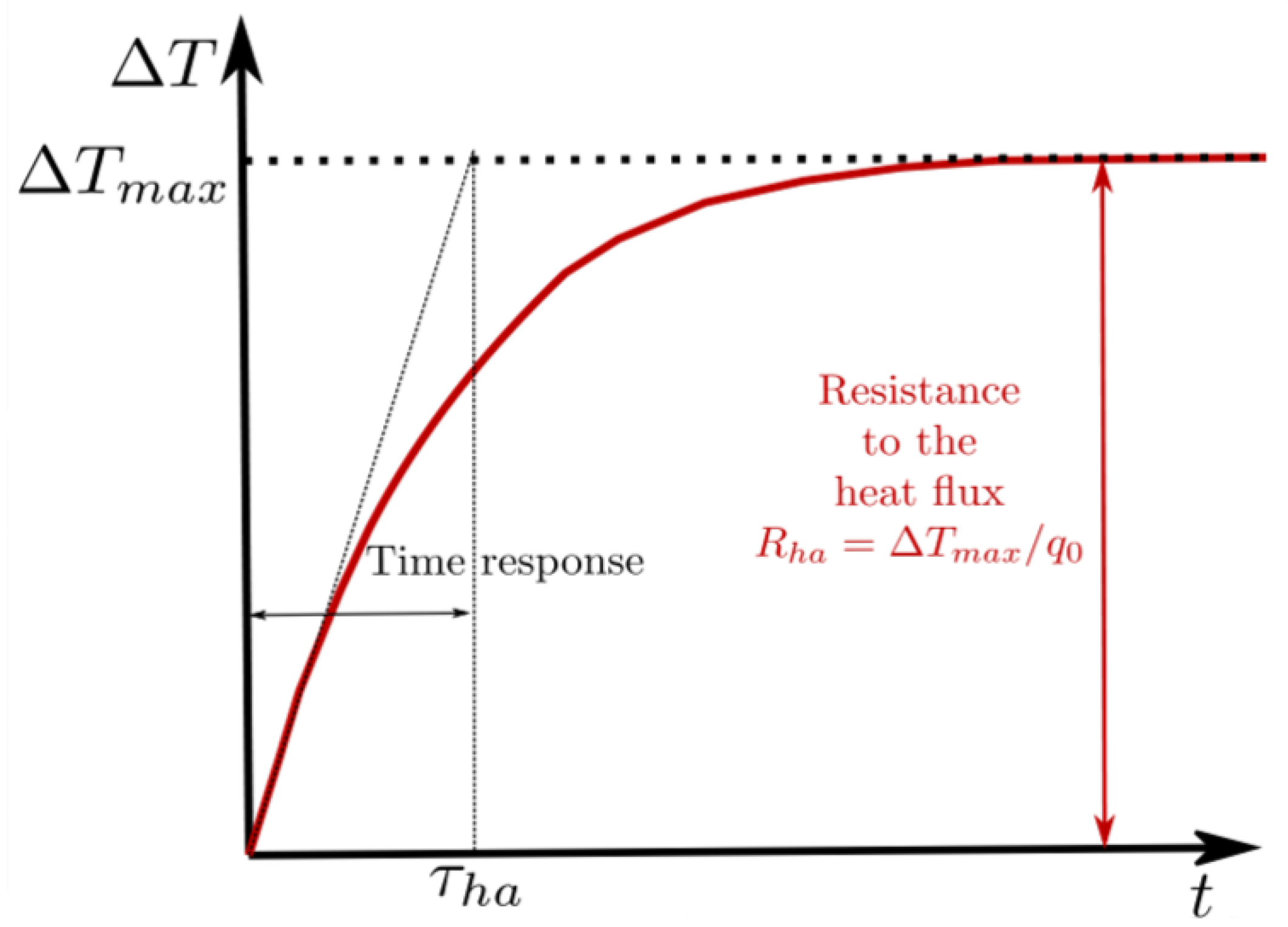
Another way of analytically modeling the temperature evolution at the wall is to use the analogy between electrical theory and thermodynamics by defining a thermal resistance and a thermal capacitor to model the temperature difference between the wall the the freestream. Figure 3 shows the temperature development in steady flow and heat flux conditions: the temperature first increases and reaches a plateau once in the steady regime.

The resistance R corresponds to the ratio between the temperature difference $\Delta T$ and the heat flux. A very resistive material corresponds to a material very sensitive to any heat flux input and the resistance R is defined by

$$\Delta T=R\times q_0$$

(3)

Any small input will lead to a very large increase in the temperature difference. Regarding the capacity C, this simply corresponds to the time response of the system to the input. This is completely analogous to electrical dynamics with the voltage (potential difference) and current passing through the resistance.

The model here developed is based on the previously described Karman–Pohlhausen’s method. Different speeds and heat fluxes are tested in steady conditions, and the values for resistances and response times $\tau =RC$ are extracted at each streamwise position x on the flat plate. This leads to an interpolated function for $R(x,q_0,U_{\infty })$ and $\tau (x,q_0,U_{\infty })$ that will be used for the resolution of the first-order differential equation:

$${\displaystyle \frac{d\Delta T}{dt}}+{\displaystyle \frac{1}{\tau (x,q_0,U_{\infty })}}\Delta T=R(x,q_0,U_{\infty })\times {\displaystyle \frac{q_0}{\tau (x,q_0,U_{\infty })}}.$$

(4)

The unsteadiness of the interaction between the heat flux $q_0$ and the speed $U_{\infty }$ is investigated using this equation with the values of R and $\tau$ calibrated with KPM. The validity of the model is discussed afterwards after the comparison with CFD in the study cases detailed in the next section.

For steady conditions on the speed and the heat flux, Equation (4) can be solved analytically, and the solution is simply written as

$$\Delta T\left(t\right)=\underset{\Delta T_{max}}{\underbrace{R{q}_0}}(1-e^{-t/\tau })$$

(5)

2.2. Numerical Validation

As a validation tool for the model, the open-source software OpenFOAM version v2306 [12] is used. The solver buoyantFoam is used in unsteady laminar flow conditions as it is able to deal with CHT problems. The mesh is a flat plate of length $a=20$ cm. It consists of two blocks of, respectively, $80\times 160$ and $160\times 160$ elements. This was chosen to be sufficiently refined, especially in the wall region. The grid requirements are not so demanding since the Reynolds number stays below 10,000 [13]. The configuration is a flat plate heated by the power loss $q_0$ and cooled down with the convective airflow.

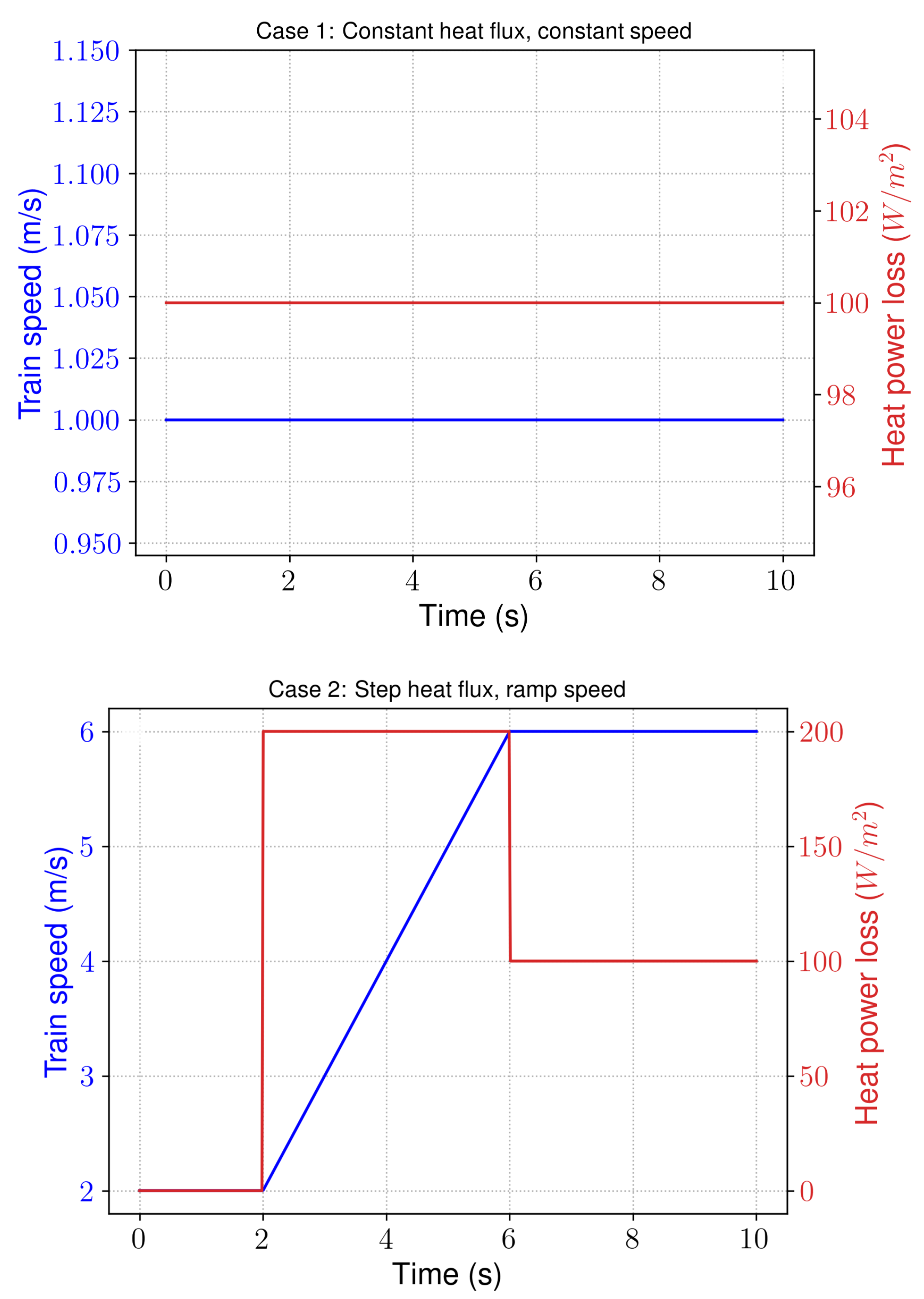
Two study cases are considered here for testing the analytical model. Figure 4 shows the two cases, representing two general driving behaviors for a train in operation:

• Case 1: A simplification of a driving behavior during cruise when the speed and the traction power are constant. It is here assumed that the train undergoes almost no elevation and that the flow conditions are favorable (no crosswind or very unsteady wind). The temperature $T_{\infty }$ represents the static temperature in the freestream in the surroundings of the train. $U_{\infty }$ is the train speed, and $T_w$ is the temperature of the wall, heated by $q_0$, the heating power dissipated. Its calculation is estimated in the next section. Case 1 aims at first validating Lachi’s method, based on Karman–Pohlhausen’s method, in comparison to CFD. Second, the values of the thermal resistance $R_{air}\left(x\right)$ and the response time ${\tau }_{air}\left(x\right)=R_{air}{C}_{air}$ are stored in a correspondence table, depending on the speed and the power loss.
• Case 2: The second case considers a simplified acceleration maneuver, where the speed increases at a constant rate until the target value, after which the speed is kept constant. The case assumes a constant mechanical power is needed for the acceleration phase in order to deal with both the running resistance and the inertial resistance. Once the target speed is reached, the mechanical power is only needed for dealing with the running resistances, so the input power is considered to be half of that in the acceleration phase. The RC model based on the correspondence table is compared to the results of CFD.

The validation of the RC model is carried out in two main steps through the two presented study cases. As explained in the presentation of the analytical model, the first step is to validate the low-order method with the CFD. This method is then used to store the thermal impedances in the RC model as functions of the streamwise position x, the heat flux input $q_0$, and the speed $U_{\infty }$. It must be noted that it runs within a few seconds, whilst the CFD needs more than two minutes. CFD is here used as our reference for the validation.

2.2.1. Case 1

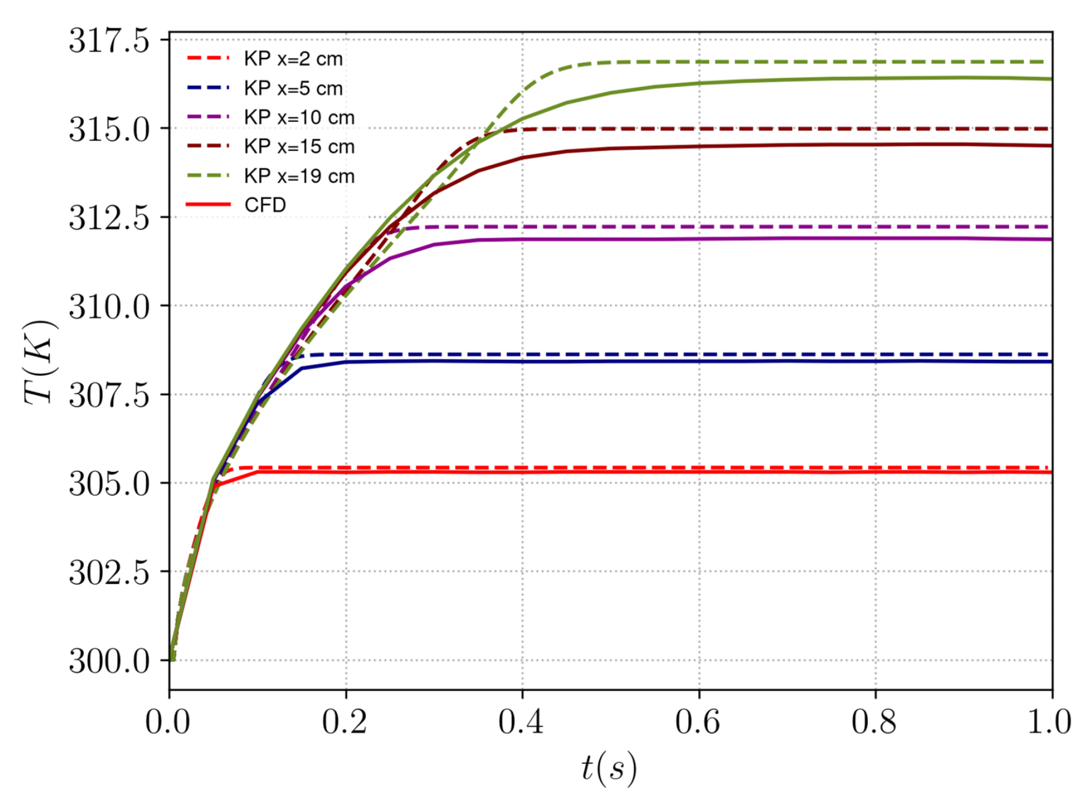
Case 1 deals with constant traction, and speed and only compares the CFD with the integral method. The results are examined at five different streamwise positions x for a flat plate of length $a=20$ cm between the KP method and CFD. The freestream temperature $T_{\infty }$ is 300 K, corresponding to a regular day in the summer. Figure 5 shows the temperature solutions to the two numerical methods. The steady values are consistent from the leading edge to the trailing edge of the plate with a slight overestimate of the KP method compared to CFD. It can be noticed that this difference increases farther down the plate. These results, however, are quite reasonable. Regarding the transient evolution, the plateau is reached sooner by the KP method and with a larger peak. The match between the two methods is good overall, with a maximum overestimate of the KP method of 1 K. The temperature seems to follow the evolution described with the RC model with an increase up to a plateau for all the axial positions.

Storage of R and C Dependencies for the Impedance Method

As explained in Section 2.1, the values for the resistance and the capacitance depend on three parameters: the axial position x, the heat flux $q_0$, and the train speed $U_{\infty }$. Three things must be emphasized here:

• The resistance and the response time do not depend on the heat flux in the range tested, that is, the range physically covered in terms of losses on converters, as shown in the next section.
• The resistance and the response time plummet with the speed. This is physically understandable since the convection improves the dissipation of the power that accumulates on the plate and in the boundary layer. Also, when the speed is larger, the response of the system is faster.
• Both the resistance and the response time increase when moving farther downstream from the leading edge.

2.2.2. Case 2

The second case only compares the RC model with the CFD. The KP method was here only used to calibrate the RC model with case 1. This time, Equation (4) is solved numerically using the correspondence table established for different speeds and heat fluxes in case 1. A function for the resistance R and the capacitance C is built upon an interpolation of that correspondence table.

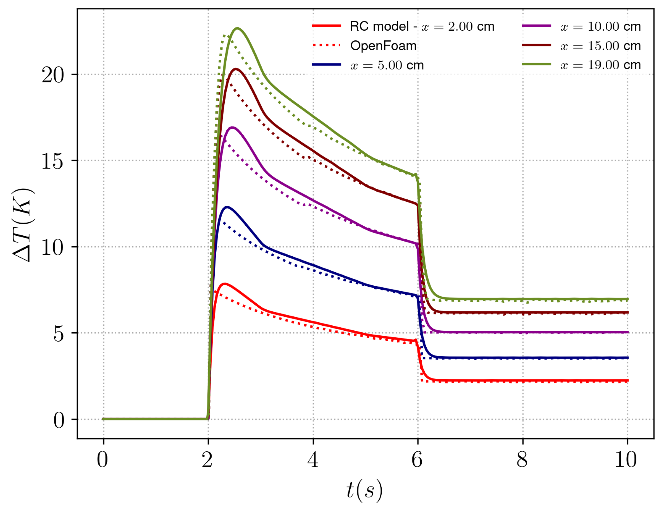
This case enables one to tackle the most common unsteadiness for a train in operation: an acceleration with larger losses followed by a plateau in speed and a reduction in the losses. The results indicated by Figure 6 show a very good agreement between the CFD and the RC model, with an overestimate during the acceleration and a slower increase (the peak is reached slightly after with the RC model). Regarding how the temperature evolves, a peak is reached, and the temperature starts decreasing when the speed balances out the heat flux input. The decrease continues, and the temperature rapidly decreases when the speed plateau is reached. A plateau on the temperature is quickly attained afterwards.

For larger speeds, a possible flow transition of the flow from laminar to turbulent flow is not accounted for by the analytical method. However, assuming a laminar flow yields an upper boundary for the temperature when passive cooling is used since turbulent flows are generally more efficient at cooling the flow [14].

3. Power Losses on the Converters

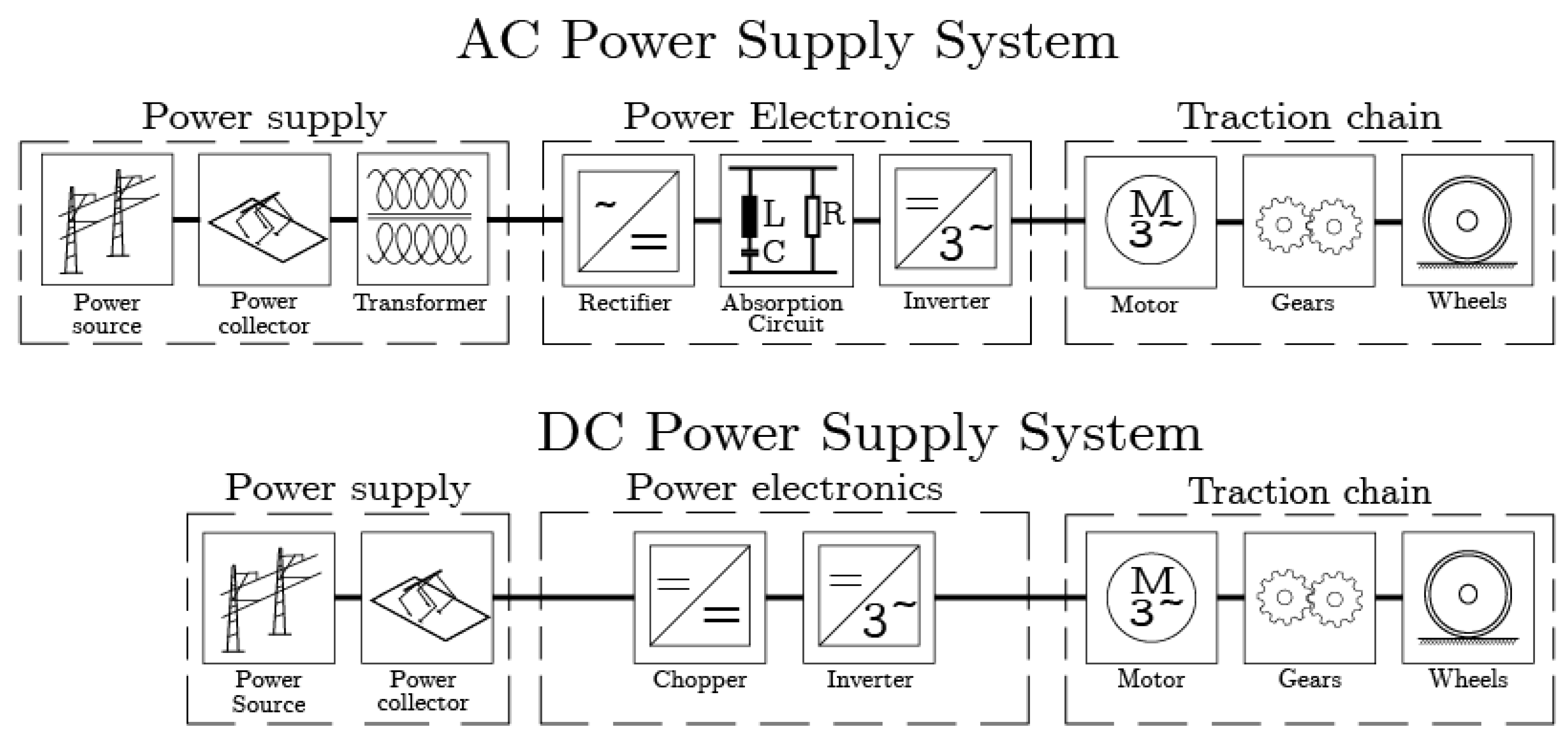
Converters are devices that convert one form of electric current to another, i.e., from Alternating Current (AC) to Direct Current (DC) or vice versa. Converters that convert the AC to DC are called rectifiers, and those converting DC to AC are called inverters. Both play a vital role in the traction chain of a rail vehicle. As represented in Figure 7, a typical traction chain of a rail vehicle consists of three parts: the power supply, the power electronics, and the traction. The components in the power supply and the power electronics will vary depending on the supply system available. In the case of an AC supply system, both rectifiers and inverters are utilized in the traction chain. In the case of a DC supply system, only the inverters are utilized in the traction chain.

In this paper, a conceptual metro train with a DC supply system has been used as an example to illustrate the model. As depicted in Figure 7, in the case of a DC supply system, the current from the catenary is transferred to the pantograph through a contact patch. If the line voltage is too high for the operation of the motor, a chopper may be inserted in the DC-intermediate part of the traction chain. The current from the pantograph or the chopper is then fed to the inverter. The inverter then converts the DC to a three-phase AC. The three-phase AC is finally used to operate the traction motor. The traction motor is connected to the wheelsets with the help of a gearbox.

3.1. Calculation of the Losses

It is here assumed that the electric motor operates in nominal conditions, at the peak value for the torque, for a fixed-supply frequency. In this section, the losses induced on the inverters are calculated.

3.1.1. Converter Losses

As mentioned in the introduction, the new possibilities offered by silicon carbide are changing the perspective in terms of converter designs. The history of the high-speed Japanese trains detailed by Sato et al. [3] shows how power electronics has improved over the last thirty years and how SiC is a big breakthrough for the sector. A figure that is worth recalling is the 30% decrease in total device energy loss per phase of the converter. This reduction in losses directly implies a reduction in the heat generated, explaining why passive cooling systems have become a possibility.

By switching on and off the inverter at a high frequency, the conversion system aims at replicating a sine signal with the right frequency in order to control the revolution speed of the rotor and the torque in the electric motor.

The losses in power electronics are due to two main sources [15]:

• Switching losses $P_{sw}$: They correspond to the amount of energy wasted in the switching on/off of the transistors and diodes of the converters. The opening and closing of these components are not perfect and some energy is lost due to the latency of these components.
• Conduction losses $P_{cond}$: They correspond to Joule’s law, relating the power lost due to the resistance of the system to the current passing through it.

The total loss can be written in Equation (6):

$$\begin{array}{cc}\hfill P_{loss}& =P_{sw}+P_{cond}\hfill \\ \hfill & =1/2V_{in}{I}_{max}{f}_s(t_{on}+t_{off})+R_d{I}_{max}^2/2\hfill \end{array}$$

(6)

$V_{in}$ represents the phase voltage, $I_{max}$ represents the peak current of the sine feeding the motor, $f_s$ represents the switching frequency of the power electronics, and $t_{on}$ and $t_{off}$ represent the respective turning-on and turning-off times. Finally, $R_d$ is the load resistance of the whole conversion system. The question is how to relate these different values to the actual traction provided by the motor at each instant.

3.1.2. Relation Between the Motor and the Converter Losses

The idea of the complete model is to use two inputs for predicting the temperature: the speed of the train and the traction power on the motors. With the traction power, it is possible to extract the torque and the revolution speed $\omega$ of the rotor. The latter can then be used to obtain the current, voltage, and switching frequency, from Figure 8, presented before.

The corresponding evolutions of the current and the voltage with the revolution speed $\omega$ enable one to calculate the total losses on the converters by using the values given by the electronics manufacturer regarding the switching frequency, the latency, and the load resistance.

3.2. Thermal Transfer from the Converters

Based on the same idea as the one used to estimate the resistance and response time of the air interaction with the heated flat plate, in the previous section, the thermal conduction through the electronic converters can be modeled by an $RC$ network. According to Ma et al. [16], power electronic devices such as the insulated-gate bipolar transistors (IGBTs) can basically be divided into two main parts: the inside module and the outside module. The inside module consists of the chip, the solder, and several layers of conductors down to the base. Below that is the outside module, where the heat sink is placed, to cool down the IGBT.

The construction of the current model is also based on Bahman et al. [17]. The coupling of the cooling with the power losses generated on the converters can be illustrated by the model in Figure 9, putting together both the power loss from the electronics and the power dissipated by convection.

The model can be summarized by the top block, representing the electronic ensemble from the conversion system to the heat sink where the temperature needs to be captured at different locations. This block has two boundary conditions:

• The heat source for the power actually lost on the electronic system, as described in the previous section.
• The cooling for the power dissipated by the interaction of the air with the heat sink.

The sketch is broken down into two parts, summarizing how both electronic and fluid models work. Using the traction power and the train speed as inputs, the power generated and the power dissipated can be used as inputs for the thermal RC network showed in the middle of the sketch. Thus, the temperature can be estimated over time at the different nodes, corresponding to the different locations of interest in between the control board and the heat sink.

After explaining here how to calculate the power losses on converters, a model for the induction motor is still needed. The losses indeed depend on the voltage and intensity of the motor when it is operating.

3.3. Electric Motor

In this paper, a three-phase squirrel cage induction motor is used in the conceptual metro train, consisting of two main parts, the stator and the rotor. The stator consists of two major components: the core and the windings. The stator core is made of laminated sheets with slots for accommodating the three-phase copper windings.

The core of the squirrel cage rotor is similarly made of thin laminated steel sheets with slots, accommodating longitudinal conductive bars typically made of aluminum or copper. These conductor bars are then connected to end rings at both ends, short-circuiting the rotor. The rotational motion of the rotor shaft is what powers the train (Figure 7).

When applying a three-phase alternating current to the stator windings placed 120° apart, it generates a rotating magnetic field (RMF), which interacts with the stationary rotor conductors, inducing an alternating current in the rotor. The two alternating fluxes, from the stator and the rotor, interact with each other, the alternating flux in the rotor lagging behind, developing an electromagnetic torque that powers the rotor.

During an operation cycle of a train, there are variations in the power demand of the motor due to the nature of the drive cycle of the train. This means the current and the voltage also vary. Since the inverters supply the motor with the required current and voltage, a variation in the power demand on the motor results in a variation in the power demand on the inverters, influencing the power losses in the inverter.

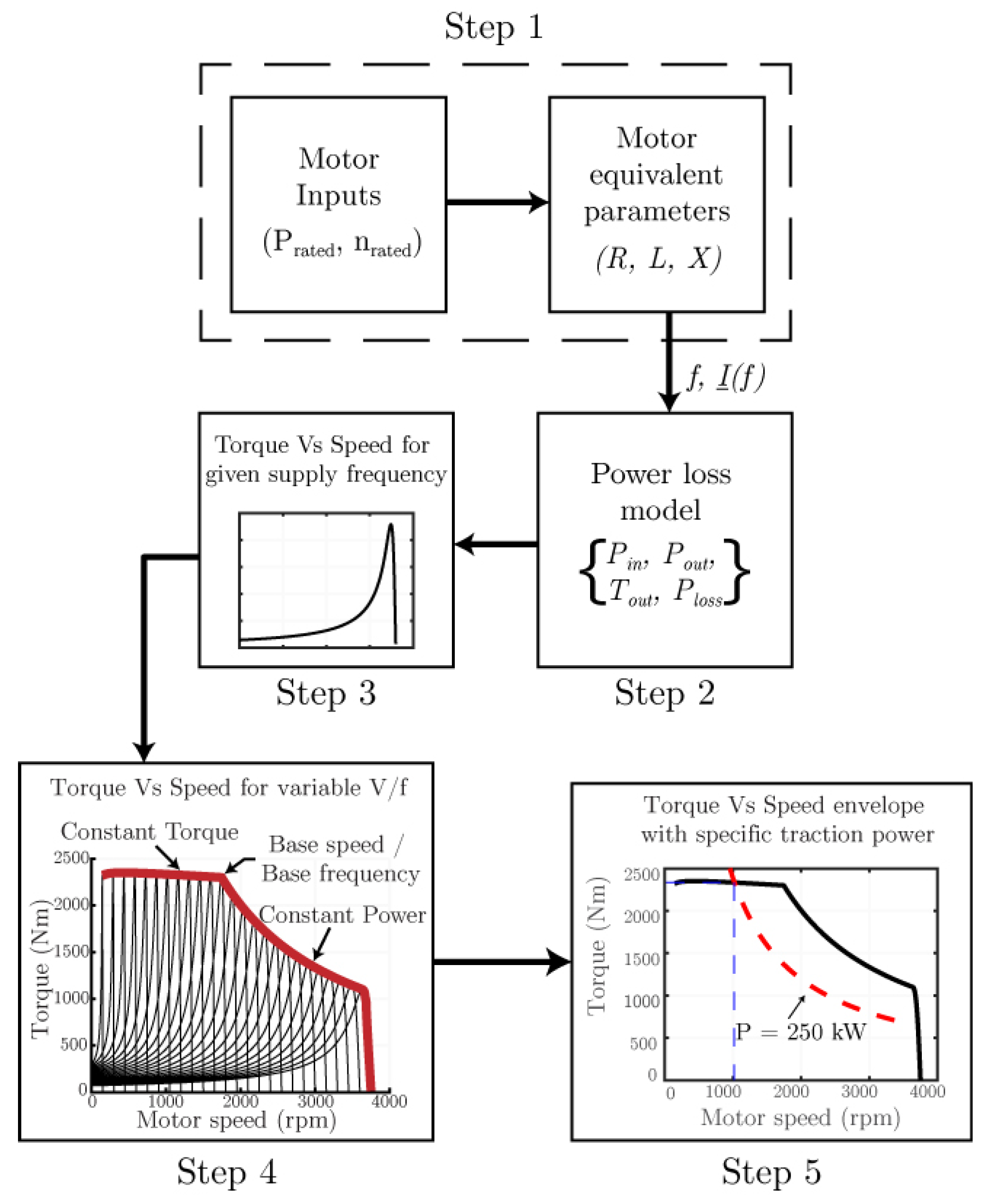
To derive these current and voltage values, an extensive motor model is developed. The method is inspired from [18,19]. It comprises five major steps as depicted in Figure 8.

In the first step, the motor equivalent parameters are calculated from the input parameters. The motor equivalent parameters include the current $\left(\underline{I}\left(f\right)\right)$, resistance $\left(R\right)$, inductance $\left(L\right)$, and reactance $\left(X\right)$ of both stator and rotor. In the second step, these equivalent parameters are used to calculate the power loss model of the motor. In the third step, this power loss model is then used to calculate the power and torque developed by the motor at one specific frequency. In the fourth step, a simple Variable–Voltage–Variable–Frequency (VVVF) control logic is implemented to obtain the power and torque developed by the motor across its entire operating range. This results in a typical torque–speed characteristics of the motor. In the fifth step, for a given traction power, the corresponding torque, speed, current, and voltage values are calculated using the developed torque–speed curve.

The torque–speed characteristic curve in step 4 contains information about current and voltage values at every operational point of the motor. For the sake of simplification, it is assumed that the motor would operate on the nominal region of the torque–speed curve, i.e., the envelope of the characteristic map. As depicted in Figure 8, a specific traction power when plotted with the torque–speed curve results in a hyperbolic curve. Therefore, for any given traction power, the hyperbolic curve intersects with the nominal torque–speed curve. This allows the calculation of the torque and speed values corresponding to the given traction power $P_{traction}=T\times \omega$. These values of power, torque, and speed are further used to interpolate the corresponding current and the voltage values used for the calculation of power loss on the inverters for any given operational point.

4. Illustration of the Model Use

4.1. Presentation of the Configuration

As an example of use, the model is applied to a single converter with the technology previously described (IGBT), onboard of a metro-like train whose life cycle and driving cycle are described in a joint report associated to the European Union project Shift2Rail, describing the project NEXTGEAR [20]. The drive cycle (speed, number of motors, and traction power) is extracted from that report as the inputs for the present model, assessing the temperature evolution of the electronic components.

The present paper focuses on a metro train with 16 induction motors with a rated power of 250 kW maximum speed of 90 km/h. It is assumed that the train is powered by the 16 motors, with exactly the same power at any time of the driving cycle. The load is equally distributed, and it is assumed that one converter drives one single motor. The losses are related to one single inverter.

The values used for the thermal impedances modeling the IGBT are taken from Ma et al.’s network model [16], simplified to a two-layer module (junction and base). The values of the IGBT used for the module, which are derived from [21] are as follows: the load resistance $R_d$ of $0.95$ m$\mathrm{\Omega }$, switching frequency $f_s$ of 20 kHz, switch on duration $t_{on}$ of 435 ns, switch off duration $t_{off}$ of 395 ns, resistance $R_{jc}$ of $0.0194$ K/W, and capacitance $C_{jc}$ of $0.1021$ J/K.

It should also be mentioned that the temperature limitation for a regular IGBT is about 423 K [21], while for a SiC electronic system, the temperature limitation would be substantially higher (>573 K). The results that will be presented on the temperature peaks.

Speed and Heat Loss

The power loss and speed over time are plotted in Figure 10 in the first 1000 s of the drive cycle. It can be noticed that the acceleration phases lead to a large increase in the losses because the motor power needed for the traction force increases the thermal losses in the power electronics. Also, it should be mentioned that the phases of speed reduction here correspond to a large elevation that the train has to withstand to maintain sufficient speed. Again, the electric motor requires more power, and the conversion system losses are thus increased. This is due to the increased torque, subsequently leading to an increase in the current and voltage amplitudes. This shows how the power loss in the inverter is heavily influenced by the operational conditions of the train such as running resistance and acceleration; thus, its trend does not directly follow the trend in train speed. The power loss represents about $0.5$% of the average traction power, corresponding to realistic values observed on metro trains [20].

4.2. Temperature Evolution

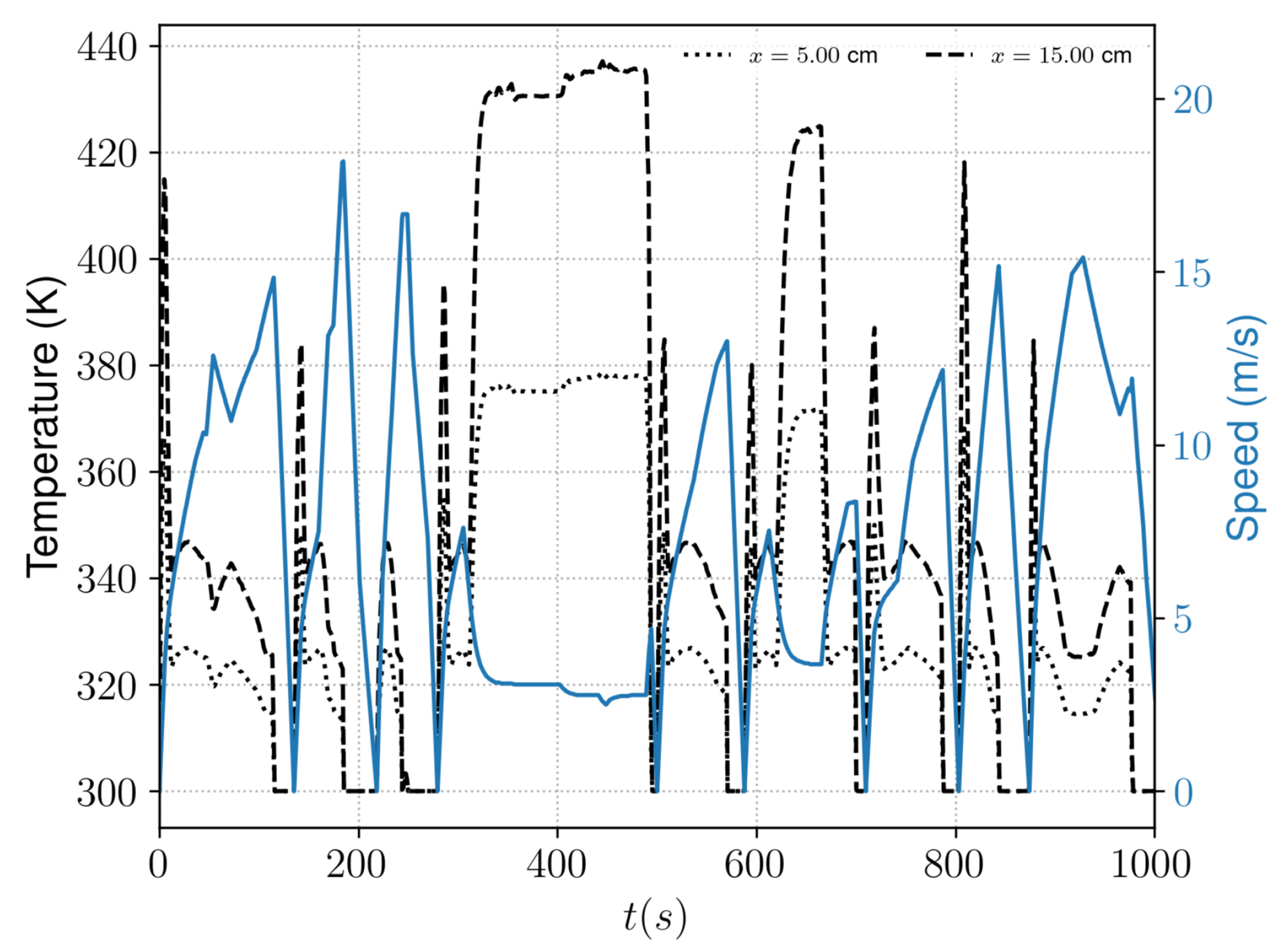
Figure 11 shows the temperature increase at two different positions of the flat plate, modeling the interaction between the bottom of the IGBT and the air. The variations are important, related to the variations of thermal losses and speed, shown before. In particular, when the speed decreases and the losses are high between 300 s and 500 s, the surge in temperature is significant, approximately 70 K at the more downstream position. At the same time, the air resistance increases abruptly with the decrease in speed and when the losses are largest: the heat loss is not as well dissipated and the temperature subsequently increases.

Figure 12 shows the evolution of the temperature at the junction at position $x=5$ cm with a clear increase in the temperature by more than 20 K compared to the base position. For a more downstream position (x = 15 cm), the model shows that the chip would overheat, with a temperature exceeding 420 K. For more efficient electronic systems, such as MOSFETs made of SiC, the temperature limitation is significantly higher [22] (around 300 K), which is a safer match with this type of passive cooling.

It must, however, be recalled that this investigation represents a non-optimal scenario in terms of cooling efficiency: the heat sink geometry is not considered, and the thermal exchanges could be increased for a better cooling. Also, laminar flow is usually less efficient than turbulent flow for cooling down by convection [14].

5. Conclusions

With the adoption of SiC power electronics, passive cooling by train-induced airflow is becoming a realistic alternative to active systems. In such systems, however, heat generation is driven by traction power, while cooling depends on train speed, leading to critical mismatches during operation. The highest power peaks, and thus the largest thermal loads, often occur during acceleration from standstill when cooling is minimal. Predicting these transient interactions requires solving a conjugate heat transfer (CHT) problem, where computational fluid dynamics is accurate but computationally costly. As predesign tools that can address this coupling are scarce in the literature, the objective of this study was to develop an analytical method to estimate the temperature evolution at the inverter surface by incorporating the main physical effects while keeping computational costs significantly lower than CFD. To demonstrate the developed method, a simplified model of a metro train inverter and a realistic operational drive cycle are used.

An electronic model of the heat loss generated by an electronic converter of a metro train has been coupled to a fluid model aiming to predict the temperature evolution in time and space on a flat plate, depending on the flow speed and the power input on the flat plate. By predicting the heat generated and the power dissipated on that flat plate, the model is able to estimate the variations of the temperature at the surface of a converter, considering the converter as a circuit of thermal impedance.

For the fluid model, an integral method has been used to calculate the variations of temperatures along a flat plate compared to CFD with a constant heat flux input and a constant airflow speed. The integral method has been used to calibrate values of an equivalent resistance and a capacitance for different speeds and heat fluxes. When the RC model is applied with the driving behavior of case 2, the results are very close to the CFD. The method has its limitations based on the assumptions made but gives promising results in terms of what can be pursued with such a method.

Such a model could be useful to state on the viability of passive cooling. The advantage of such a method is clearly its cost: if the error made on the temperature variations, particularly temperature peaks, can be properly evaluated, a possibility of adapting this type of models to assess whether passive cooling is sufficient on different designs of converters and driving configurations. Again, CFD is still very challenging in that regard for industrials.

The results depict that there are higher losses during acceleration and larger temperature surges of around 70 K at lower speeds. Additionally, the temperature variation at the junction at $x=5$ cm is 20 K higher than at the base position, and the junction temperature exceeds 420 K further downstream at $x=15$ cm. This indicates that the developed method is able to capture the temperature variations with sufficient accuracy across the flat plate configuration considering several physical effects influencing the thermal exchange at the surface of the inverter.

As further work, the temperature increase given by the model presented in the paper should be compared with actual data in the future. It should also be noticed that using a heat sink would improve the efficiency of cooling compared to a simple flat plate, but further work should be carried out on analytically modeling the interaction with the air to be used in the same perspective as in the present model (thermal impedance associated). Moreover, accounting for turbulent conditions would also impact the results in terms of cooling. If laminar flows can be seen as a worst-case scenario in terms of passive cooling efficiency, a better predesign approach could go further by modeling turbulent flows, but the problem to be solved is even more complex.

References

1. Siemens. Silicon Carbide—A Material That Developers Dream About. 2024. Available online: https://www.mobility.siemens.com/global/en/company/stories/silicon-carbide-a-material-that-developers-dream-about.html (accessed on 25 August 2025).
2. Lindahl, M.; Trostén, T.; Jansson, D.; Johansson, M.H.; Velander, E.; Blomberg, A.; Nee, H. Field Test of a Silicon Carbide Metro Propulsion System with Reduced Losses and Acoustic Noise. IET Electr. Syst. Transp. 2021, 11, 47–57. [Google Scholar] [CrossRef]
3. Sato, K.; Kato, H.; Fukushima, T. Development of SiC Applied Traction System for Shinkansen High-Speed Train. In Proceedings of the 2018 International Power Electronics Conference (IPEC-Niigata 2018 -ECCE Asia), Niigata, Japan, 20–24 May 2018; IEEE: Piscataway, NJ, USA, 2018; pp. 3478–3483. [Google Scholar]
4. Sato, K.; Kato, H.; Fukushima, T. Outstanding Technical Features of Traction System in N700S Shinkansen New Generation Standardized High-Speed Train. IEEJ J. Ind. Appl. 2021, 10, 402–410. [Google Scholar] [CrossRef]
5. Wang, Y.; Dai, X.; Liu, G.; Wu, Y.; Li, D.; Jones, S. Integrated Liquid Cooling Automotive IGBT Module for High Temperatures Coolant Application. In Proceedings of the PCIM Europe 2015, International Exhibition and Conference for Power Electronics, Intelligent Motion, Renewable Energy and Energy Management, Nuremberg, Germany, 19–20 May 2015; pp. 1–7. [Google Scholar]
6. Fukushima, T.; Kameda, T. Train-Draft-Cooling Power Converters for Bullet Trains: A Blowerless Converter/Inverter, n.d. Available online: https://www.jsme.or.jp/jsme/uploads/2016/11/awardn09-05.pdf (accessed on 25 August 2025).
7. Lienhard, J.H. Heat Transfer in Flat-Plate Boundary Layers: A Correlation for Laminar, Transitional, and Turbulent Flow. J. Heat Transf. 2020, 142, 061805. [Google Scholar] [CrossRef]
8. He, L.; Oldfield, M.L.G. Unsteady Conjugate Heat Transfer Modeling. J. Turbomach. 2011, 133, 031022. [Google Scholar] [CrossRef]
9. Mathie, R.; Nakamura, H.; Markides, C.N. Heat Transfer Augmentation in Unsteady Conjugate Thermal Systems—Part II: Applications. Int. J. Heat Mass Transf. 2013, 56, 819–833. [Google Scholar] [CrossRef]
10. Volkov, V.N. A Refinement of the Karman–Pohlhausen Integral Method in Boundary Layer Theory. J. Eng. Phys. 1965, 9, 371–374. [Google Scholar] [CrossRef]
11. Lachi, M.; Rebay, M.; Mladin, E.C.; Padet, J. Alternative Models for Transient Convection Heat Transfer in External Flows over a Plate Exposed to a Variable Heat Flux. Int. J. Therm. Sci. 2004, 43, 809–816. [Google Scholar] [CrossRef]
12. Greenshields, C.; Weller, H. OpenFOAM|Free CFD Software|The OpenFOAM Foundation. 2024. Available online: https://openfoam.org/ (accessed on 25 August 2025).
13. Pope, S.B. Turbulent Flows; Cambridge University Press: Cambridge, UK, 2015. [Google Scholar]
14. Afrid, M.; Zebib, A. Three-Dimensional Laminar and Turbulent Natural Convection Cooling of Heated Blocks. Numer. Heat Transf. Part A 1991, 19, 405–424. [Google Scholar] [CrossRef]
15. Ghaviha, N.; Holmberg, C.; Bohlin, M.; Dahlquist, E. Modeling of Losses in the Motor Converter Module of Electric Multiple Units for Dynamic Simulation Purposes. Energy Procedia 2017, 142, 2303–2309. [Google Scholar] [CrossRef]
16. Ma, K.; Xu, M.; Liu, B. Modeling and Characterization of Frequency-Domain Thermal Impedance for IGBT Module Through Heat Flow Information. IEEE Trans. Power Electron. 2021, 36, 1330–1340. [Google Scholar] [CrossRef]
17. Bahman, A.S.; Ma, K.; Blaabjerg, F. A Lumped Thermal Model Including Thermal Coupling and Thermal Boundary Conditions for High-Power IGBT Modules. IEEE Trans. Power Electron. 2018, 33, 2518–2530. [Google Scholar] [CrossRef]
18. Boldea, I.; Nasar, S.A. The Induction Machines Design Handbook, 2nd ed.; CRC Press/Taylor & Francis: Boca Raton, FL, USA, 2010. [Google Scholar]
19. Pyrhonen, J.; Jokinen, T.; Hrabovcová, V. Design of Rotating Electrical Machines, 2nd ed.; Wiley: Chichester, UK, 2014. [Google Scholar]
20. NEXT Generation Methods, Concepts and Solutions for the Design of Robust and Sustainable Running GEAR|NEXTGEAR Project|Fact Sheet|H2020. December 2023. Available online: https://cordis.europa.eu/project/id/881803/results (accessed on 25 August 2025).
21. Backlund, B.; Schnell, R.; Schlapbach, U.; Fischer, R.; Tsyplakov, E. Applying IGBTs; Application Note 5SYA2053-01; ABB Switzerland Ltd.: Baden, Switzerland, 2007. [Google Scholar]
22. Lostetter, A.; Hornberger, J.; McPherson, B.; Reese, B.; Shaw, R.; Schupbach, M.; Rowden, B.; Mantooth, A.; Balda, J.; Otsuka, T.; et al. High-Temperature Silicon Carbide and Silicon on Insulator Based Integrated Power Modules. In Proceedings of the 2009 IEEE Vehicle Power and Propulsion Conference, Dearborn, MI, USA, 7–10 September 2009; IEEE: Piscataway, NJ, USA, 2009; pp. 1032–1035. [Google Scholar]
Figure 1. Illustration of the conjugate heat transfer on a conductive slab heated by a flux q w and submerged into a steady flow of freestream velocity U .
Machines 13 00788 g001
Figure 3. Development of the temperature for a constant heat flux on the flat plate with a steady flow.
Machines 13 00788 g003
Figure 4. Speed and heat power loss over time for the two cases of study. For case 1, the values represented are used for the validation between Lachi’s method and CFD.
Machines 13 00788 g004
Figure 5. Temperature evolution over time for case 1 at five different axial positions of the plate. Comparison between CFD (solid lines) and Karman–Pohlhausen’s method (dashed lines).
Machines 13 00788 g005
Figure 6. Temperature difference evolution over time for case 2 at five different axial positions of the plate. Comparison between RC model (solid lines) and CFD (dashed lines).
Machines 13 00788 g006
Figure 7. Typical representation of a traction chain of a rail vehicle with an AC supply system and a DC supply system.
Machines 13 00788 g007
Figure 8. Outline of the procedure followed in motor model.
Machines 13 00788 g008
Figure 9. Illustration of the coupling model to estimate the temperature evolution on the converters.
Machines 13 00788 g009
Figure 10. Speed and traction power used for the study.
Machines 13 00788 g010
Figure 11. Temperature evolution over time at two different positions of the flat plate.
Machines 13 00788 g011
Figure 12. Temperature evolution over time at the base and the junction for x = 5 cm.
Machines 13 00788 g012
Disclaimer/Publisher’s Note: The statements, opinions and data contained in all publications are solely those of the individual author(s) and contributor(s) and not of MDPI and/or the editor(s). MDPI and/or the editor(s) disclaim responsibility for any injury to people or property resulting from any ideas, methods, instructions or products referred to in the content.