Fault Classification in Power Transformers Using Dissolved Gas Analysis and Optimized Machine Learning Algorithms

Abstract

Power transformers are critical assets in electrical power systems, yet their fault diagnosis often relies on conventional dissolved gas analysis (DGA) methods such as the Duval Pentagon and Triangle, Key Gas, and Rogers Ratio methods. Even though these methods are commonly used, they present limitations in classification accuracy, concurrent fault identification, and manual sample handling. In this study, a framework of optimized machine learning algorithms that integrates Chi-squared statistical feature selection with Random Search hyperparameter optimization algorithms was developed to enhance transformer fault classification accuracy using DGA data, thereby addressing the limitations of conventional methods and improving diagnostic precision. Utilizing the R2024b MATLAB Classification Learner App, five optimized machine learning algorithms were trained and tested using 282 transformer oil samples with varying DGA gas concentrations obtained from industrial transformers, the IEC TC10 database, and the literature. The optimized and assessed models are Linear Discriminant, Naïve Bayes, Decision Trees, Support Vector Machine, Neural Networks, k-Nearest Neighbor, and the Ensemble Algorithm. From the proposed models, the best performing algorithm, Optimized k-Nearest Neighbor, achieved an overall performance accuracy of 92.478%, followed by the Optimized Neural Network at 89.823%. To assess their performance against the conventional methods, the same dataset used for the optimized machine learning algorithms was used to evaluate the performance of the Duval Triangle and Duval Pentagon methods using VAISALA DGA software version 1.1.0; the proposed models outperformed the conventional methods, which could only achieve a classification accuracy of 35.757% and 30.818%, respectively. This study concludes that the application of the proposed optimized machine learning algorithms can enhance the classification accuracy of DGA-based faults in power transformers, supporting more reliable diagnostics and proactive maintenance strategies.

1. Introduction

With the increased expansion of power system transmission and distribution networks worldwide due to the adaptation of renewable energy, it is essential to retain the reliability of the critical and expensive equipment used in the network. One such piece of equipment is the power transformer. Power transformers ensure that power is transmitted and distributed at correct voltage ranges for efficient and value-engineered operation from generation stations to end-users. To ensure continuous operation of the transformers, their condition must be continuously monitored. One of the most commonly adopted methods used to achieve this is through the transformer’s insulating oil via the dissolved gas analysis (DGA) method [1]. DGA is a transformer condition monitoring technique that tracks the presence of dissolved gasses in the insulating transformer oil [2]. Gasses such as Methane (CH₄), Ethane (C₂H₆), Ethylene (C₂H₄), Acetylene (C₂H₂), Hydrogen (H₂), Carbon Monoxide (CO), and Carbon Dioxide (CO₂) are present in the transformer at varying concentrations, with a combination of these gasses signifying certain incipient faults that the transformer is susceptible to [3,4,5,6,7]. For detection of incipient electrical faults, the indicative assessed gas combination consists of Acetylene, Hydrogen, and Methane, while for incipient thermal faults, the assessed gasses are Methane, Ethane, Ethylene, Hydrogen; lastly, for insulation breakdown, the gasses that are assessed are Carbon Monoxide and Carbon Dioxide [8]. The DGA oil extraction and gas detection procedure used to carry out the analysis is as follows [9].

• A specialized sampling syringe is used to cautiously extract a small uncontaminated oil sample from a transformer oil sampling valve located at the bottom part of a transformer and transfer it into a gas-tight container.
• The sampled oil is taken to a laboratory where any present gasses are extracted from it using techniques such as headspace extraction or vacuum extraction.
• Gas chromatographic analysis is then conducted to analyze, identify, and categorize gasses present in the extracted oil as gas concentration measured in parts per million (ppm).
• The gas concentrations of the detected gasses are then used for interpreting the results to assess the transformer condition and flag incipient faults using DGA-based interpretation techniques.

Over the past few decades, conventional methods such as the Duval Triangle and Pentagon, CIGRE method, Key Gas Ratios, Dornenberg, IEC Ratio, and Rogers Ratio Methods have been used for DGA interpretation and condition monitoring of transformers. These methods proved to be effective but only to a certain extent [9,10,11,12,13,14,15]. Various studies indicate that these methods exhibit limitations and inconsistencies due to manual handling of results, the significant difference in accuracies between the methods, and the inability of these methods to simultaneously diagnose different incipient faults present in transformers and detect any borderline incipient faults. These limitations are reported to be associated with each method’s poor adaptability when presented with complex and imbalanced gas concentrations, and with fixed classification thresholds set out by industrial specifications [1,2,9,10,11,12,13,14,15].

As a result, this instils uncertainty pertaining to the accuracy of the results obtained using these methods, despite how often they have been effectively used to a certain extent for transformer fault diagnosis. In recent research work on the transformer condition monitoring niche, the application of machine learning methods for transformer fault classification based on conventional DGA interpretation methods has been explored by researchers intending to improve the transformer fault classification shortcomings presented by the conventional methods [4,16,17]. Table 1 shows a summary of recent related works that have been conducted by researchers in the area of machine learning and transformer diagnosis based on DGA.

Table 1. Summary of recent related works.

Ref.	Cites	Year	ML Algorithm	ML Dataset Source	Contributions and Developments
[18]	102	2019	Improved Krill Herd SVM	IEC TC10 and Private Company	A fault diagnosis Improved Krill Herd optimized SVM algorithm based on cross-validation scheme; achieved an accuracy of 85.71%.
[19]	31	2024	Deep CNN	Literature	A fault classification asset management technique based on a Deep Convolutional Neural Network for the prediction of transformer’s health index; the technique achieved an accuracy of 87%.
[20]	96	2021	Teaching-learning based optimization	Egyptian Electricity Holding Company	A teaching-learning-based optimization technique for transformer fault diagnosis using dissolved gas concentration limits and the conventional method gas ratios; the technique achieved an accuracy of 86.27%.
[21]	53	2021	Gaussian Process Multiclassification	General Electric	A probabilistic interpretation technique for analyzing DGA results using the Gaussian Process Multiclassification to enhance the analysis.
[22]	196	2015	SVM	IEC TC10	An optimized SVM model using Generic Algorithm-based optimum gas ratios; the model achieved an accuracy of 87.18%.
[23]	99	2017	Bayesian networks	IEC TC10	A Bayesian network probabilistic fault diagnosis framework incorporating hypothesis testing for DGA; the technique achieved a diagnosis accuracy of 88.9%.
[24]	122	2017	SVM and kNN	IEC TC10	An SVM and kNN particle swarm-optimized technique based on Duval’s Pentagon 1 method used for fault diagnosis against the faults detected in transformer oil; this technique achieved an accuracy of 88%.
[25]	60	2020	SVM	Electrical Utilities	A transformer fault severity detection technique based on the SVM and Duval Pentagon method; it achieves this by incorporating gas properties and DGA interpretation criterion at an accuracy of 88%.
[26]	15	2020	GAPSVM	State Grid Corporation of China and IEC TC10	A combination of SVM and Generic Algorithm-optimized techniques that is integrated with a fuzzy three-ratio technique for fault detection; this technique achieved an accuracy of 86.8%.
[27]	78	2021	ANN	Egyptian Electricity Transmission Company	A combination of all the conventional DGA techniques, and it uses the output of the analysis as an input to an Artificial Neural Network algorithm for refined incipient fault detection; this technique achieved an accuracy of 84.96%.

Table 1. Summary of recent related works.

Ref.	Cites	Year	ML Algorithm	ML Dataset Source	Contributions and Developments
[18]	102	2019	Improved Krill Herd SVM	IEC TC10 and Private Company	A fault diagnosis Improved Krill Herd optimized SVM algorithm based on cross-validation scheme; achieved an accuracy of 85.71%.
[19]	31	2024	Deep CNN	Literature	A fault classification asset management technique based on a Deep Convolutional Neural Network for the prediction of transformer’s health index; the technique achieved an accuracy of 87%.
[20]	96	2021	Teaching-learning based optimization	Egyptian Electricity Holding Company	A teaching-learning-based optimization technique for transformer fault diagnosis using dissolved gas concentration limits and the conventional method gas ratios; the technique achieved an accuracy of 86.27%.
[21]	53	2021	Gaussian Process Multiclassification	General Electric	A probabilistic interpretation technique for analyzing DGA results using the Gaussian Process Multiclassification to enhance the analysis.
[22]	196	2015	SVM	IEC TC10	An optimized SVM model using Generic Algorithm-based optimum gas ratios; the model achieved an accuracy of 87.18%.
[23]	99	2017	Bayesian networks	IEC TC10	A Bayesian network probabilistic fault diagnosis framework incorporating hypothesis testing for DGA; the technique achieved a diagnosis accuracy of 88.9%.
[24]	122	2017	SVM and kNN	IEC TC10	An SVM and kNN particle swarm-optimized technique based on Duval’s Pentagon 1 method used for fault diagnosis against the faults detected in transformer oil; this technique achieved an accuracy of 88%.
[25]	60	2020	SVM	Electrical Utilities	A transformer fault severity detection technique based on the SVM and Duval Pentagon method; it achieves this by incorporating gas properties and DGA interpretation criterion at an accuracy of 88%.
[26]	15	2020	GAPSVM	State Grid Corporation of China and IEC TC10	A combination of SVM and Generic Algorithm-optimized techniques that is integrated with a fuzzy three-ratio technique for fault detection; this technique achieved an accuracy of 86.8%.
[27]	78	2021	ANN	Egyptian Electricity Transmission Company	A combination of all the conventional DGA techniques, and it uses the output of the analysis as an input to an Artificial Neural Network algorithm for refined incipient fault detection; this technique achieved an accuracy of 84.96%.

Even though the mentioned methods have been effective to a certain degree in their application, these methods have indicated limitations and challenges associated with the uncertainty of the results due to manual handling of the test samples, the accuracy of the methods, the inability to concurrently diagnose existing transformer faults, and the identification of transformer incipient faults. These limitations and challenges prompted the adaptation of machine learning techniques to resolve these issues; however, despite the application of these intelligent approaches, the literature shows that they exhibit deficiencies related to accurately classifying faults based on the DGA data. To address the classification and diagnostic precision limitation presented by the conventional interpretation methods, this study notably contributed by developing a framework of optimized machine learning algorithms that integrates the Chi-squared statistical feature selection with the Random Search hyperparameter optimization algorithms for transformer fault classification using dissolved gas analysis. This entailed training and testing five optimized machine learning algorithms using the Classification Learner App in MATLAB. The performance of these algorithms was then assessed against the conventional Duval Triangle and Duval Pentagon methods using the VAISALA DGA software.

2. Materials and Methods

This section outlines the materials and methods used to conduct this study. It discusses the DGA data collection method, the frameworks used for developing the transformer faults multiclassification optimized machine learning models, the software used to conduct this study, and the evaluation metrics used to assess the performance of the models.

2.1. Machine Learning Model Development

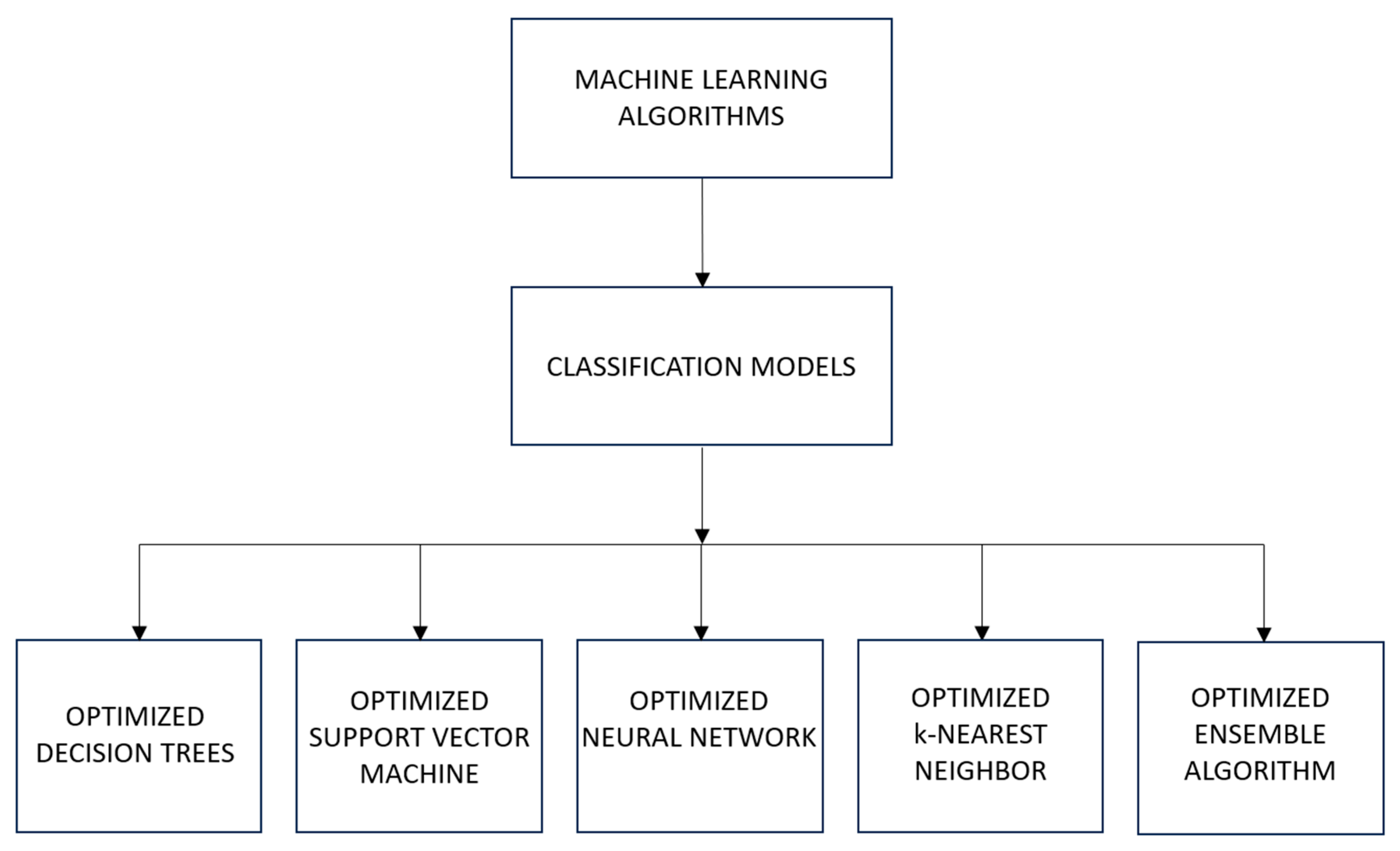
In general, machine learning consists of various algorithms used for various purposes grouped into 2 main methods, supervised learning and unsupervised learning, which are further collapsed into 3 groups, i.e., classification and regression for supervised learning, and clustering for unsupervised learning. However, for this study, supervised learning classification algorithms were adopted for the classification of transformer faults based on gas concentrations obtained from dissolved gas analysis chromatography tests. The classification machine learning algorithms used in this study for transformer fault classification are Decision Trees, Support Vector Machine, Neural Networks, k-Nearest Neighbor, and the Ensemble Algorithm.

Table 2. Machine learning classification algorithms.

Classifier	Model	Description
Decision Trees	Mdl = fitctree(Tbl, ResponseVarName) [28]	The fitctree function trains a fitted Decision Tree model using the defined predictors (dissolved gases), contained in the DGA dataset table “Tbl” and “ResponseVarName”, i.e., labeled fault classes, contained in the DGA dataset [28].
Support Vector Machine	Mdl = fitcecoc(Tbl, ResponseVarName) [29,30]	The fitcecoc function trains a Support Vector Machine model using the defined predictors (dissolved gases) and labeled fault classes of the DGA dataset where the function uses K(K − 1)/2, with “K” being the number of labeled fault classes [29,30].
Neural Networks	Mdl = fitcnet(Tbl, ResponseVarName) [31]	The fitcnet function trains a Neural Network model using the defined predictors (dissolved gases), contained in the DGA dataset table “Tbl” and “ResponseVarName”, i.e., labeled fault classes, contained in the DGA dataset [31].
k-Nearest Neighbor	Mdl = fitcknn(Tbl, ResponseVarName) [32]	The fitcknn function trains a k-Nearest Neighbor model using the defined predictors (dissolved gases), contained in the DGA dataset table “Tbl” and labeled fault classes in the variable “Tbl.ResponseVarName” [32].
Ensemble Algorithm	Mdl = fitcensemble(Tbl, ResponseVarName) [33]	The fitcensemble function trains the model based on the resultsboosting classification trees along with the defined predictors (dissolved gases), contained in the DGA dataset table “Tbl” and “ResponseVarName”, i.e., labeled fault classes, contained in the DGA dataset. The function achieves this using the AdaBoostM2 (Adaptive boosting) algorithm for multiclassification [33].

shows a summary of the machine learning algorithms and their functions used in this study, and the diagram in Figure 1 shows the machine learning algorithms considered for this study.

2.2. MATLAB/Classification Learner for Machine Learning Model Development

To address the transformer fault classification problem presented in this study using machine learning algorithms, a model structure that comprises Input variables, Validation schemes, Predictors, Responses, optimized algorithms, feature selection, and optimization was developed. Figure 2 shows the proposed scheme and experimental setup model, where 282 DGA samples are used in the models. Furthermore, evaluation methods such as the confusion matrix, accuracy, precision, recall, F1-score, and Receiver Operating Characteristic Curve and Area Under Curve (ROC-AUC curves) were used to assess the performance of the models.

2.2.1. Data Collection

A practical cumulated DGA dataset obtained from the IEC TC 10 database, the literature, and a South African Industrial Transformer Manufacturer is presented in this study for classifying transformer faults using machine learning algorithms. This dataset consists of 282 transformer oil samples, where an 80:20 partition ratio was used, i.e., 80% of the dataset was used for training the models and 20% was used for testing the models. Numerically, 226 samples were for training and 56 for testing the optimized machine learning algorithms in the MATLAB Classification Learner App. From these 282 samples, there are 55 D1 fault samples, 77 D2 fault samples, 100 NF no-fault samples, 36 T1 fault samples, and 14 T3 fault samples. The samples collected from the various sources are compiled into an Excel format and imported into MATLAB Workspace via MATLAB Drive in the correct format. In the Classification Learner App, the dataset is then called in from the Workspace environment, updated, and the Response and Predictors are selected based on the dataset labels. Furthermore, the dataset was used in the VAISALA DGA Calculator software to test the performance of the conventional methods, i.e., Duval Triangle and Duval Pentagon, for comparison against the proposed optimized machine learning algorithms. An extracted sample of the DGA dataset is shown in Appendix A,

Table A1. DGA samples extracted from used dataset.

H2 (ppm)	CH4 (ppm)	C2H6 (ppm)	C2H4 (ppm)	C2H2 (ppm)	Fault Type
305	100	33	161	541	D1
35	6	3	26	482	D1
543	120	41	411	1880	D1
57	24	2	27	30	D1
1000	500	1	400	500	D1
440	89	19	304	757	D2
210	43	12	102	187	D2
2850	1115	138	1987	3675	D2
5000	1200	83	1000	1100	D2
10,000	6730	345	7330	10,400	D2
1570	735	87	1330	1740	D2
6709	10,500	1400	17,700	750	T3
290	966	299	1810	57	T3
2500	10,500	4790	13,500	6	T3
860	1670	30	2050	40	T3
107	143	34	222	2	T3
6729	323	2323	45,353	2	D1
10,000	800	222	9	40	D1
9900	780	150	10	35	D1
9823	707	231	8	4	D1
9531	744	220	8	7	D1
9840	788	225	9	40	D1
9032	785	219	12	38	D1
30	80	675	220	3	T1
4000	6076	4544	23,232	2	T1
4317	5898	4781	22,212	5	T1
4133	5902	4608	20,449	4	T1
4051	5507	4330	22,825	3	T1
4262	5856	4689	22,286	2	T1
100	200	188	3222	1212	NF
400	380	5800	400	2	NF
100	40	2311	335	6	NF
953	737	465	39	464	NF

.

2.2.2. Validation Scheme

The model was based on inputs where the best performing combinations were taken into consideration, which included the evaluation of the various validation schemes for selection, namely the cross-validation, holdout validation, and re-substitution validation schemes. Ultimately, the k-fold validation was chosen for application in this proposed model for protection against overfitting, and the dataset was cross-validated into 20 folds to increase confidence and evaluation performance in the model following a series of trial–error runs to determine the most optimum value between cross-validation and holdout validation. Re-substitution was omitted on the onset due its inability to provide protection overfitting and the fact that it used the same dataset samples for training and testing, indicating that it does not partition the samples. For the performance comparison of the different validation schemes tested, see

Table A2. Machine learning validation schemes performance comparison.

Validation Scheme	Metric	Algorithm
		kNN	NN	SVM	Ensemble	Tree
Cross	Accuracy (%)	92.48	89.82	83.19	82.301	80.53
	Precision (%)	91.80	89.61	83.94	84.03	82.37
	Recall (%)	91.38	89.53	81.62	79	78.83
	F1-score (%)	91.54	89.52	82.04	79.25	79.67
Hold-out	Accuracy (%)	85.71	82.14	73.2	82.14	82.14
	Precision (%)	86.78	85.23	81.62	82.49	82.49
	Recall (%)	84.9	82.80	71.21	74.90	74.9
	F1-score (%)	82.82	80.86	73.20	76.08	76.08

in Appendix A. The results show that cross-validation has a better overall performance compared to hold-out.

2.2.3. Predictors and Responses

From the DGA samples, only the H₂, CH₄, C₂H₂, C₂H₄, and C₂H₆ gasses were considered predictors to determine the condition of the transformers. The omitted CO and CO₂ are generally used when assessing the condition of the insulating paper. From DGA samples with labeled faults, the faults that the models were trained and tested against are the low and high energy discharges (D1 and D2), thermal faults (T1, T2, and T3), partial discharge (PD), and no-fault condition (NF).

2.2.4. Feature Selection and Optimization

For this dataset, the Chi-squared (Chi2) statistical feature selection algorithm was used for training the models. This comes at the back end of numerous pre-analysis trial-and-error runs conducted to assess and determine the best performing feature selection algorithm between the Chi2 algorithm, ReliefF algorithm, ANOVA algorithm, and Kruskal–Wallis algorithm. The Chi2 algorithm is effective in determining the essential features required for predicting a classification, and in this study, it assesses the scores of the input features H₂, CH₄, C₂H₂, C₂H₄, and C₂H₆.

For further optimization, similarly to the feature selection function, the Random Search hyperparameter optimization algorithm was chosen as the preferred optimizer after numerous pre-analysis trial-and-error runs conducted to assess and determine the best performing optimizer between the Random Search Optimization, Grid Search Optimization, and Bayesian Optimization. This optimization method was selected following a consistent accuracy performance regardless of the number of iterations the model was trained and tested against. In terms of the number of iterations, they were varied from 30 to 500 at an increment of 150%, the model yielded similar results throughout, with a difference of less than 1% but for a much longer training time (7.05 s vs. 184.64 s). For the performance comparison of the different feature selection algorithms and hyperparameter optimizers tested, see Appendix A,

Table A3. Machine learning feature selection algorithms performance comparison.

Feature Selection	Metric	Algorithm
		kNN	NN	SVM	Ensemble	Tree
Chi2	Accuracy (%)	92.48	89.82	83.19	82.301	80.53
	Precision (%)	91.80	89.61	83.94	84.03	82.37
	Recall (%)	91.38	89.53	81.62	79	78.83
	F1-score (%)	91.54	89.52	82.04	79.25	79.67
ReliefF	Accuracy (%)	92.01	88.5	77.43	85.4	80.1
	Precision (%)	88.90	86.79	84.94	82.11	76.94
	Recall (%)	89.43	84.08	72.58	81.01	71.87
	F1-score (%)	89.13	85.12	76.26	80.84	72.80
ANOVA	Accuracy (%)	92.04	86.73	82.30	88.05	80.09
	Precision (%)	88.90	85.34	79.75	91.92	76.94
	Recall (%)	89.43	82.26	75.18	80.26	71.87
	F1-score (%)	89.13	83.45	76.78	83.50	72.80
Kruskal–Wallis	Accuracy (%)	92.92	88.05	81.86	86.28	80.09
	Precision (%)	90.66	85.28	77.79	82.23	76.94
	Recall (%)	90.22	86.49	73.52	76.13	71.87
	F1-score (%)	90.33	85.78	74.88	77.37	72.80

and

Table A4. Machine learning hyperparameter optimization performance comparison.

Hyperparameter Optimization	Metric	Algorithm
		kNN	NN	SVM	Ensemble	Trees
Random Search	Accuracy (%)	92.48	89.82	83.19	82.301	80.53
	Precision (%)	91.80	89.61	83.94	84.03	82.37
	Recall (%)	91.38	89.53	81.62	79	78.83
	F1-score (%)	91.54	89.52	82.04	79.25	79.67
Grid Search	Accuracy (%)	92.92	90.71	78.76	87.17	80.09
	Precision (%)	90.66	88.13	86.33	83.32	76.94
	Recall (%)	90.20	87.04	69.58	82.63	71.87
	F1-score (%)	90.33	87.55	72.75	82.44	72.80
Bayesian	Accuracy (%)	92.36	80.09	80.09	84.96	80.09
	Precision (%)	90.66	83.47	87.21	88.73	76.94
	Recall (%)	90.20	76.00	70.95	76.24	71.87
	F1-score (%)	90.33	78.56	74.08	78.79	72.80

, respectively. The results show that the Chi-squared statistical feature selection algorithm and Random Search hyperparameter optimizer has a better over performance compared to the other feature selection and hyperparameter algorithms when compared to the others.

2.3. Performance Metrics Used for Evaluation of Models

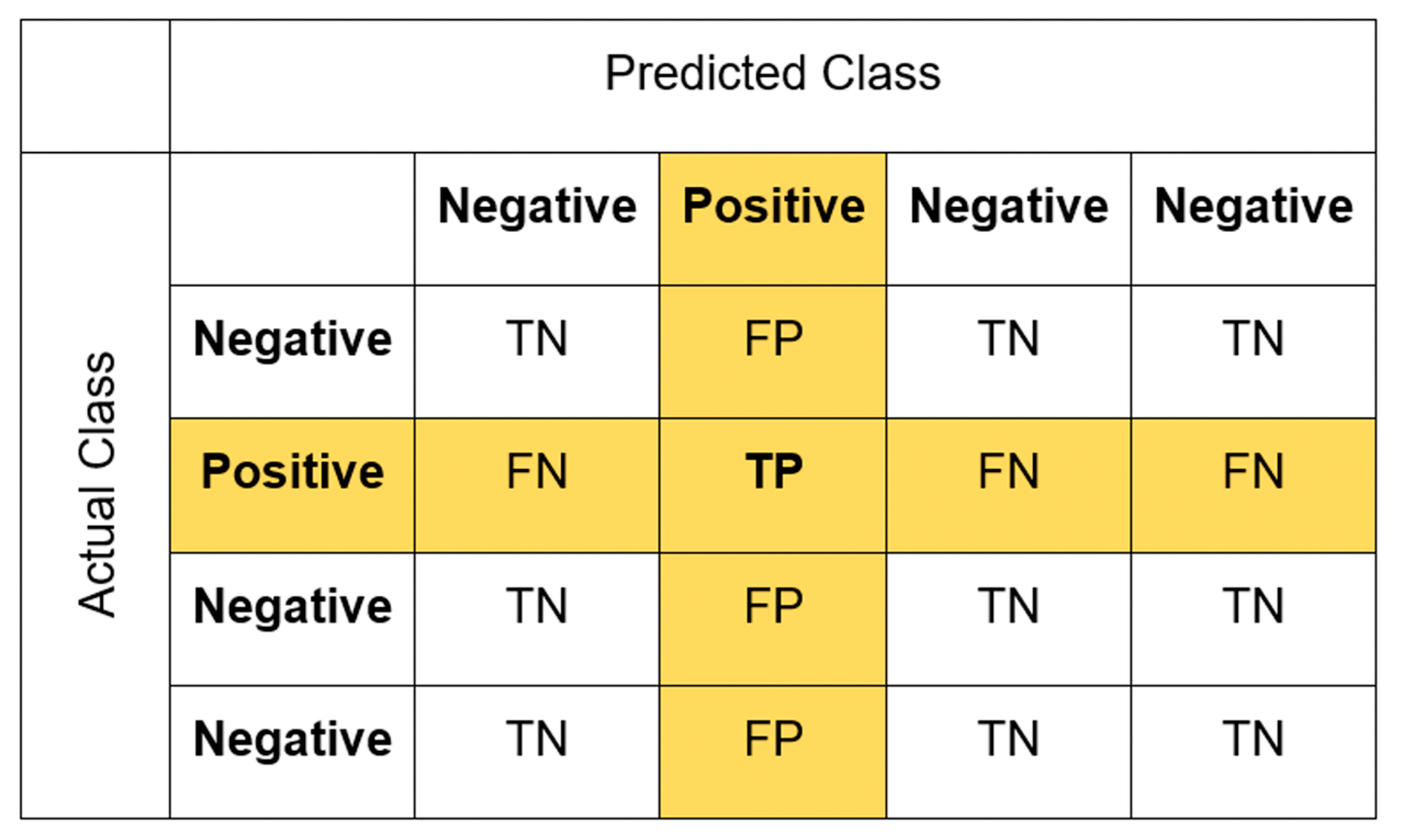
To evaluate the performance of the machine learning algorithms, various methods were adopted. Firstly, confusion matrices were used to visually assess the multiclassification performance of the algorithms. Using the true positive (TP), true negative (TN), false positive (FP), and fault negative (FN) results of the multiclassification confusion metrics, other key performance evaluation metrics, i.e., accuracy, precision, recall, and F1-score, are calculated using Equations (1)–(4). Figure 3 shows the fundamental principle of a multiclass confusion matrix, from which all the other performance matrices are calculated.

2.3.1. Accuracy

In a multiclassification evaluation problem, the accuracy performance metric denotes the proportion of samples correctly predicted in conjunction with the total number of predictions made by the model [34]. Equation (1) shows the equation used to calculate accuracy.

Accuracy = (TP + TN)/(TP + TN + FP + FN)

(1)

2.3.2. Precision

Precision is the positive prediction value accuracy performance metric that denotes the proportion of samples correctly predicted among all the correctly predicted samples [34]. Equation (2) shows the equation used to calculate precision.

Precision = TP/(TP + FP)

(2)

2.3.3. Recall

Recall is the true positive rate performance metric that evaluates anomalies that are correctly classified by the model [34]. Equation (3) shows the equation used to calculate recall.

Recall = TP/(TP + FN)

(3)

2.3.4. F1-Score

F1-score is the cumulative mean of recall and precision that provides an overview of the metrics that stabilize the recall and precision evaluation measures [34]. Equation (4) shows the equation used to calculate the F1-score.

F1-scores= (2 × Recall × Precision)/(Recall + Precision)

(4)

2.3.5. Receiver Operating Characteristics Curve and Area Under Curve

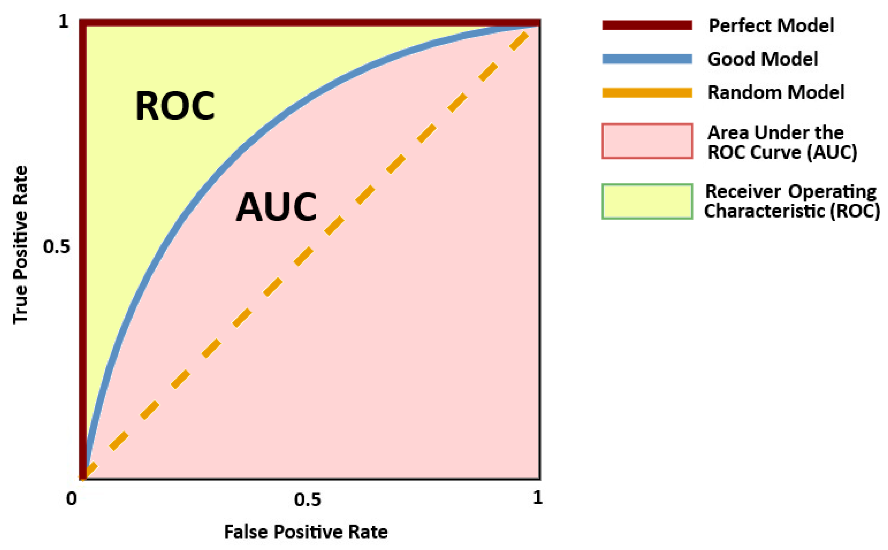
To further assess the performance of the models, the Receiver Operating Characteristic (ROC) curve is used. For the ROC curves, the true positive rate (TPR) and false positive rate (FPR) predicted by the confusion matrix of the studied model are compared to plot the different thresholds of the model’s classification scores. In the MATLAB’s Classifier Learner App that was utilized in this study, the rocmetrics function was used to plot the ROC curve.

Generally, the ROC curves are used for binary classification models, but since this study assesses a multiclassification problem, the Classifier Learner App calculates one binary problem for each DGA gas by formulating a set of one-versus-all binary classification problems, and computes an ROC curve for every class using the respective binary problem [35,36]. Additionally, to measure the overall quality of the models using the ROC curve, the Area Under Curve (AUC) value is used. This is the value that corresponds to the true positive rate values with respect to the false positive rate values ranging from 0 to 1, where the model’s good performance is indicated by values closer to 1 [35,36]. Figure 4 shows a typical ROC and AUC curves and their performance measurement matrix adapted from [37].

2.4. Performance Comparison Against Conventional Methods Using VAISALA DGA Calculator Software

For this study, to assess the performance of conventional methods, the Duval Triangle and Duval Pentagon DGA interpretation methods were tested using the VAISALA DGA Calculator software, which classifies DGA samples based on the gas concentration presented in parts per million (ppm). The results obtained using this software were then used for comparison against the results of the proposed optimized machine learning algorithms. Figure 5 shows the user interface of the VAISALA DGA Calculator software.

3. Results

In this section, the results of the optimized machine learning algorithms and the Regularized Neural Network are discussed. The chapter then compares the results of the proposed optimized machine learning algorithms against the results of the Duval Triangle and Pentagon, which were obtained using the same dataset as the proposed models. The classification results of the machine learning algorithms are presented in the form of the evaluation matrix, confusion matrices, and ROC-AUC curves. The performance of each algorithm is discussed.

3.1. Modeling of Optimized Machine Learning Algorithms’ Results

A total of 282 transformer DGA samples were used for the study, where 80% of the oil samples were used for training the models, and 20% were used for testing the models. A total of five optimized algorithms were evaluated using the same dataset in MATLAB/Classification Learner. For computation, all the studies were evaluated in 30 iterations with no time limit to allow for complete training without early stops. Overall, the results obtained from the algorithms varied in terms of performance, considering the classification accuracy shown in the confusion matrices, precision, recall, F1-score, training time, and ROC-AUC curves.

3.1.1. Optimized Ensemble Algorithm

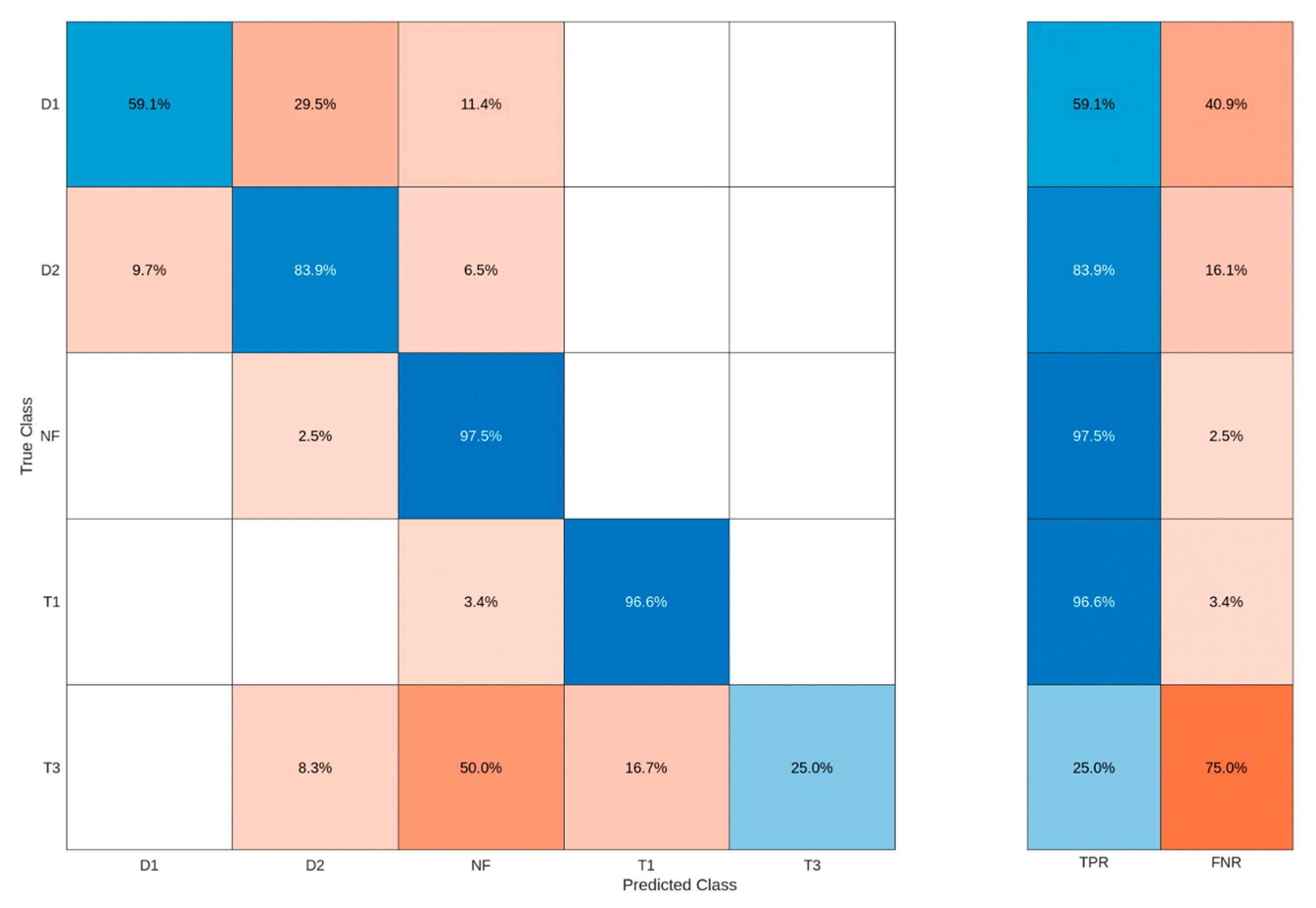
For the Optimized Ensemble algorithm shown in Figure 6, the model achieved an overall performance accuracy of 82.301% for the correctly classified dissolved gas analysis faults. The model correctly classified 59.1% as D1 fault, 83.9% as D2 fault, 97.5% as No fault, 96.6% as T1 fault, and only 25% as T3 fault. However, for the D1 fault, the model incorrectly classified 29.5% of it as a D2 fault, and 11.4% as a No fault. For the D2 fault, it incorrectly classified 9.7% as a D1 fault and 6.5% as a No fault. For the no-fault condition, it incorrectly classified 2.5% as a D1 fault. For the T1 fault, it incorrectly classified 3.4% as a No fault. Lastly, for the T3 fault, the model incorrectly classified 8.3% as a D2 fault, 50% as a No fault, and 16.7% as a T1 fault.

3.1.2. Optimized k-Nearest Neighbor Algorithm

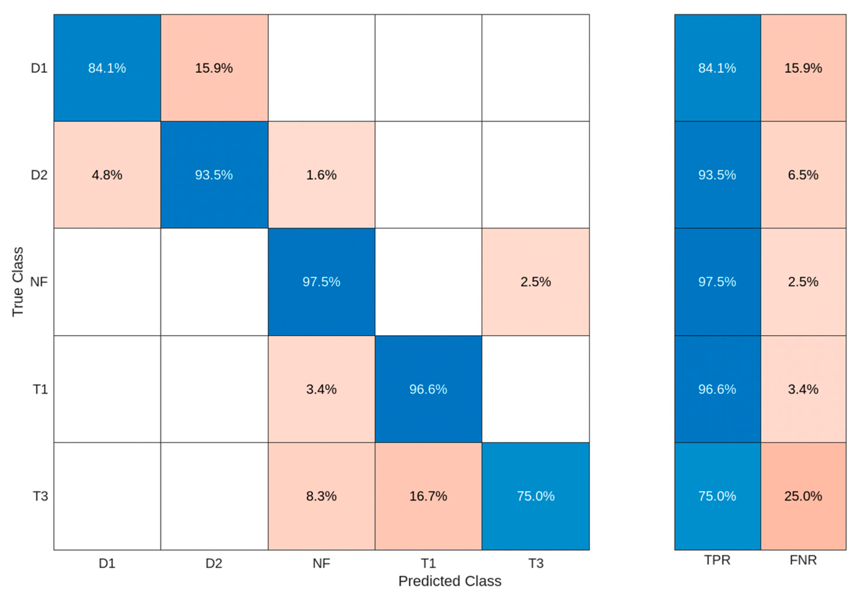
For the Optimized k-Nearest Neighbor algorithm shown in Figure 7, the model achieved an overall best performance accuracy of 92.478% for the correctly classified dissolved gas analysis faults. The model correctly classified 84.1% as D1 fault, 93.5% as D2 fault, 97.5% as No fault, 96.6% as T1 fault, and 75% as T3 fault. However, for the D1 fault, the model incorrectly classified 15.9% of it as a D2 fault. For the D2 fault, it incorrectly classified 4.8% as a D1 fault and 1.6% as a No fault. For the no-fault condition, it incorrectly classified 2.5% as a T3 fault. For the T1 fault, it incorrectly classified 3.4% as a No fault. Lastly, for the T3 fault, the model incorrectly classified 8.3% as a no-fault condition and 16.7% as a T1 fault.

3.1.3. Optimized Neural Network Algorithm

For the Optimized Neural Network algorithm shown in Figure 8, the model achieved an overall performance accuracy of 89.823% for the correctly classified dissolved gas analysis faults. The model correctly classified 81.8% as D1 fault, 91.9% as D2 fault, 91.1% as No fault, 96.6% as T1 fault, and 83.3% as T3 fault. However, for the D1 fault, the model incorrectly classified 13.6% of it as a D2 fault, 2.3% as a No fault, and 2.3% as a T1 fault. For the D2 fault, it incorrectly classified 4.8% as a D1 fault and 3.2% as a No fault. For the no-fault condition, it incorrectly classified 1.3% as a D1 fault and 5.1% as a D2 fault, and 2.5% as a T3 fault. For the T1 fault, it incorrectly classified 3.4% as a No fault. Lastly, for the T3 fault, the model incorrectly classified 8.3% as a No fault and 8.3% as a T1 fault.

3.1.4. Optimized Support Vector Machine Algorithm

For the Optimized Support Vector Machine algorithm shown in Figure 9, the model achieved an overall performance accuracy of 83.186% for the correctly classified dissolved gas analysis faults. The model correctly classified 59.1% as D1 fault, 82.3% as D2 fault, 96.2% as No fault, 96.6% as T1 fault, and 58.3% as T3 fault. However, for the D1 fault, the model incorrectly classified 29.5% of it as a D2 fault and 11.4% as a No fault. For the D2 fault, it incorrectly classified 3.2% as a D1 fault and 14.5% as a No fault. For the no-fault condition, it incorrectly classified 1.3% as a T1 fault and 2.5% as a T3 fault. For the T1 fault, it incorrectly classified 3.4% as a No fault. Lastly, for the T3 fault, the model incorrectly classified 8.3% as a D2 fault, 25% as a No fault, and 8.3% as a T1 fault.

3.1.5. Optimized Tree Algorithm

For the Optimized Tree algorithm shown in Figure 10, the model achieved an overall performance accuracy of 80.531% for the correctly classified dissolved gas analysis faults. The model correctly classified 59.1% as D1 fault, 79% as D2 fault, 92.4% as No fault, 96.6% as T1 fault, and 50% as T3 fault. However, for the D1 fault, the model incorrectly classified 34.1% of it as a D2 fault and 6.8% as a No fault. For the D2 fault, it incorrectly classified 9.7% as a D1 fault, 9.7% as a No fault, and 1.6% as a T1 fault. For the no-fault condition, it incorrectly classified 2.5% as a D1 fault and 5.1% as a D2. For the T1 fault, it incorrectly classified 3.4% as a No fault. Lastly, for the T3 fault, the model incorrectly classified 25% as a D2 fault and 25% as a no-fault condition.

3.2. Receiver Operating Characteristics Curve and Area Under Curve Results

For further analysis of the optimized models, the Receiver Operating Characteristic (ROC) curve and Area Under Curve (AUC) matrices were utilized to assess the performance of the models where the true positive rate (TPR) and false positive rate (FPR) predicted by the confusion matrices of the studied models are compared to plot the different thresholds of the model’s classification scores [35]. This was combined with the Area Under Curve (AUC) value that measures the overall quality of the model using the ROC curve. This value corresponds to the true positive rate values with respect to the false positive rate values ranging from 0 to 1, where the model’s good performance is indicated by values closer to 1 [35]. MATLAB’s Classifier Learner App was utilized to plot these curves.

3.2.1. Optimized Ensemble ROC-AUC Curve

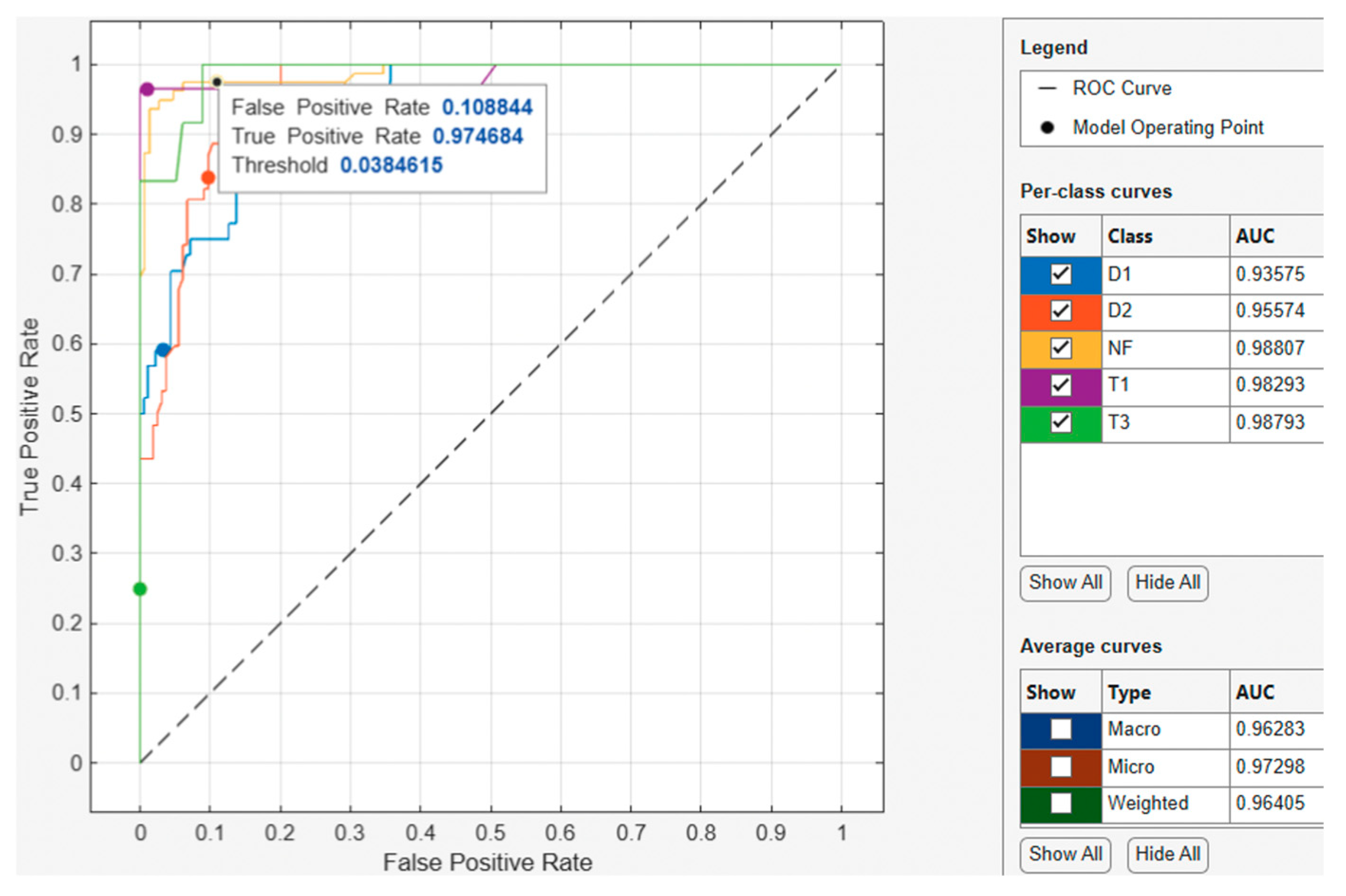
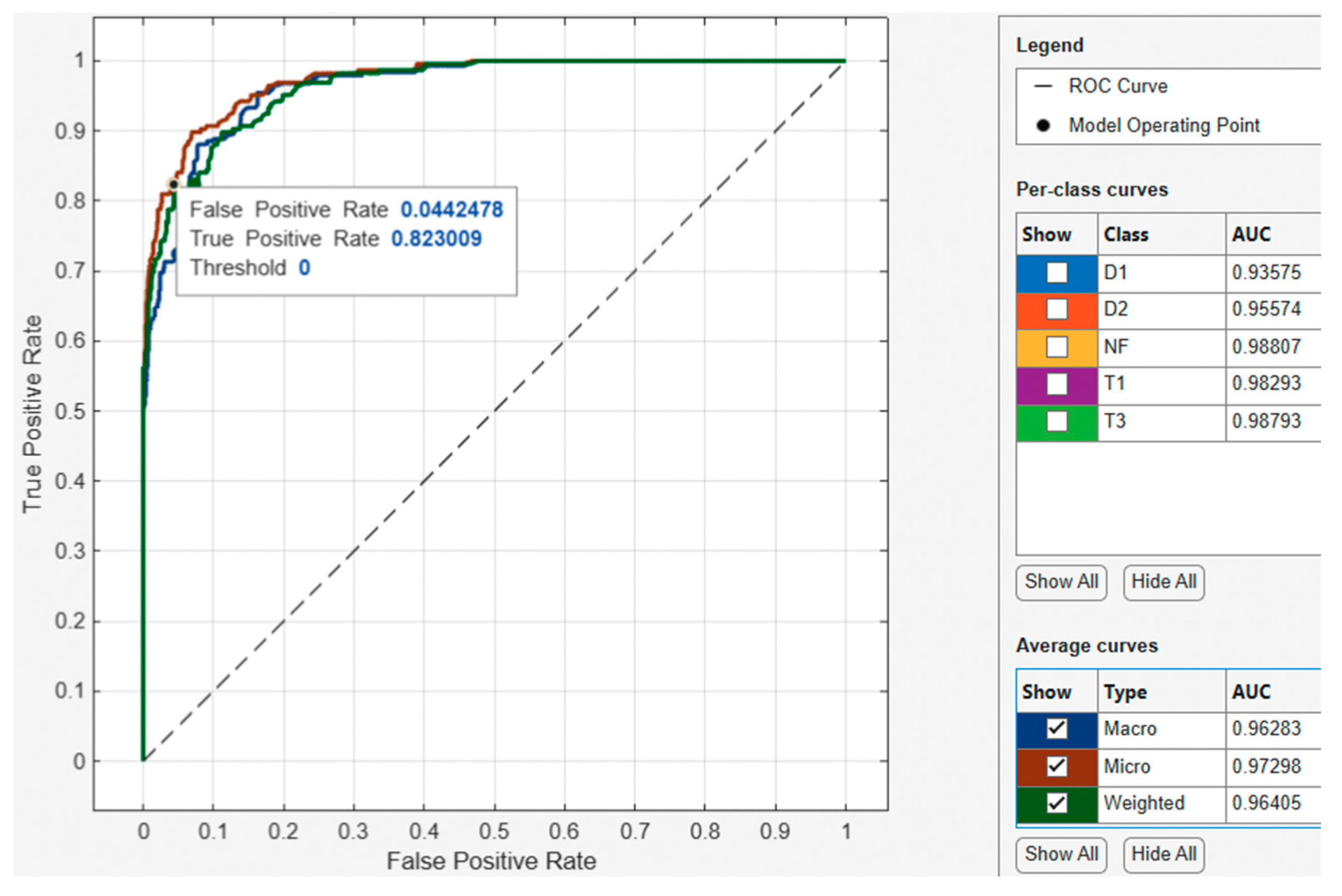
For the Optimized Ensemble model ROC-AUC curve shown in Figure 11, the model operating point with a threshold of 0.0384615 used by the classifier to classify this observation shows the corresponding true positive rate of 0.974684 and false positive rate of 0.108844. This indicates that a false positive rate of 0.1088 incorrectly classified 2.64% of the negative class observations to the positive class, and a true positive rate of 0.9 correctly classified 90% of the positive class. Regarding the AUC, the best performing class achieved an AUC value of 0.98807, which is close to the best value of 1. Furthermore, when assessing the best performing average curve in Figure 12, the classifier used a threshold of 0 for the model operating point to classify observations with a corresponding true positive rate of 0.823009 and false positive rate of 0.0442478. This indicates that the false positive rate of 0.0442 of the best performing average curve incorrectly classified 17.7% of the negative class observations as the positive class. Overall, the average curve has an AUC value of 0.97298, which is close to the best value of 1.

3.2.2. Optimized k-Nearest Neighbor ROC-AUC Curve

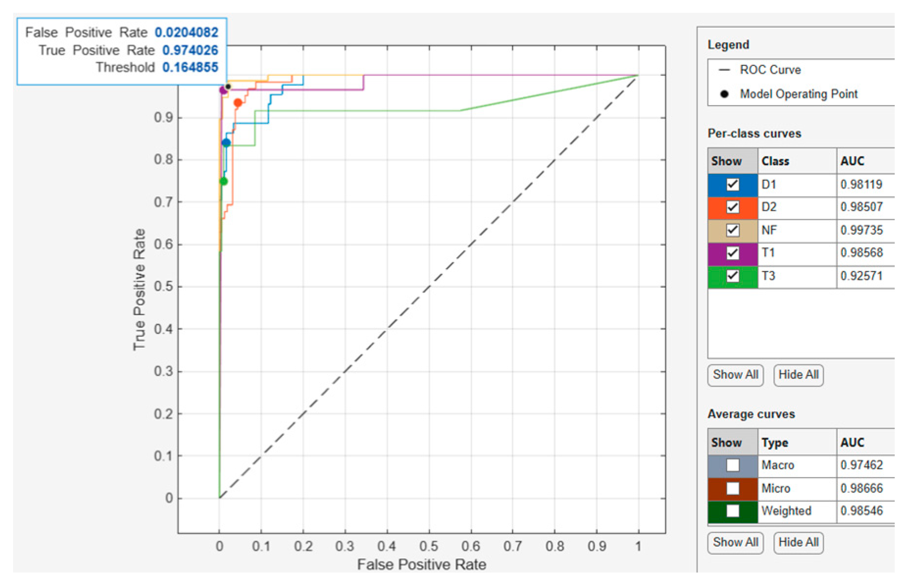
For the optimized k-Nearest Neighbor model ROC-AUC curve shown in Figure 13, the model operating point with a threshold of 0.164855 used by the classifier to classify this observation shows the corresponding true positive rate of 0.974026 and false positive rate of 0.0204082. This indicates that a false positive rate of 0.02 incorrectly classified 2.6% of the negative class observations to the positive class, and a true positive rate of 0.9 correctly classified 90% of the positive class. Regarding the AUC, the best performing class achieved an AUC value of 0.99735, which is close to the best value of 1. 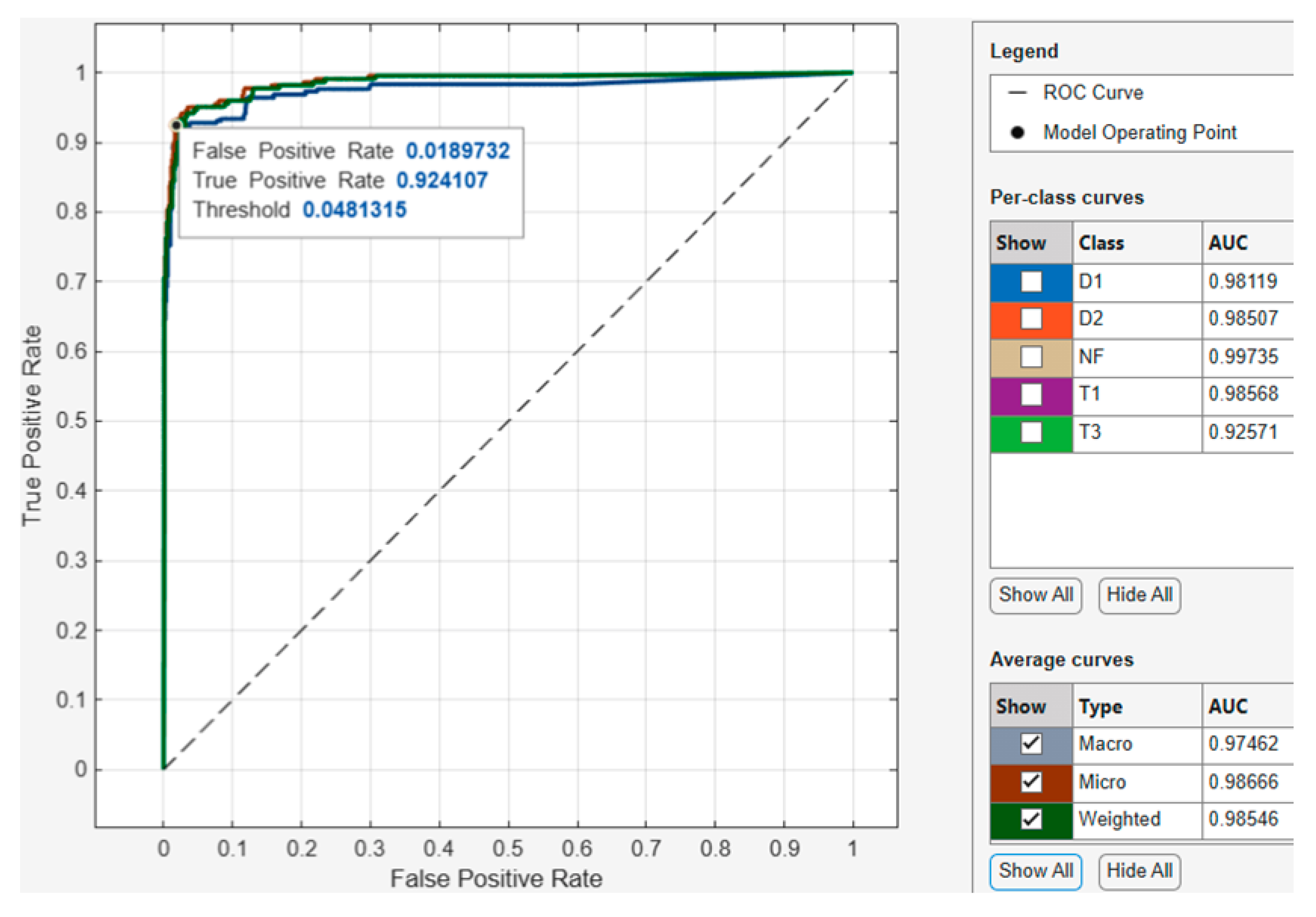Furthermore, when assessing the best performing average curve in Figure 14, the classifier used a threshold of 0.0481315 for the model operating point to classify observations with a corresponding true positive rate of 0.924107 and false positive rate of 0.0189732. This indicates that the false positive rate of 0.0189732 of the best performing average curve incorrectly classified 7.6% of the negative class observations to the positive class. Overall, the average curve has an AUC value of 0.98666, which is close to the best value of 1.

3.2.3. Optimized Neural Network ROC-AUC Curve

For the Optimized Neural Network model ROC-AUC curve shown in Figure 15, the model operating point with a threshold of 0.175352 used by the classifier to classify this observation shows the corresponding true positive rate of 0.911392 and false positive rate of 0.0340136. This indicates that a false positive rate of 0.034 incorrectly classified 8.87% of the negative class observations to the positive class, and a true positive rate of 0.9 correctly classified 90% of the positive class. Regarding the AUC, the best performing class achieved an AUC value of 0.98106, which is close to the best value of 1. 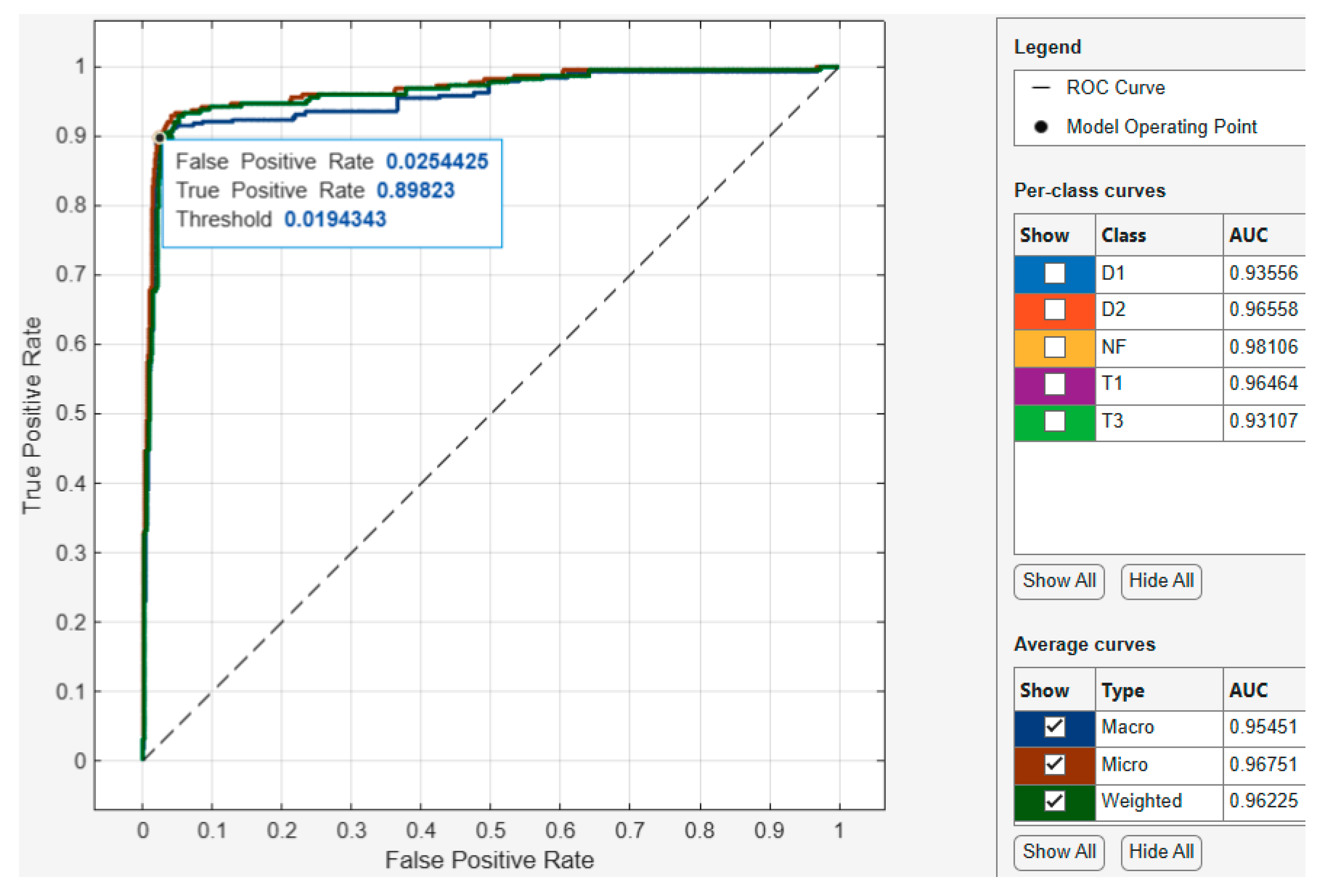Furthermore, when assessing the best performing average curve in Figure 16, the classifier used a threshold of 0.0194343 for the model operating point to classify observations with a corresponding true positive rate of 0.89823 and false positive rate of 0.0254425. This indicates that the false positive rate of 0.0254 of the best performing average curve incorrectly classified 10.28% of the negative class observations as the positive class. Overall, the average curve has an AUC value of 0.96751, which is close to the best value of 1.

3.2.4. Optimized Support Vector Machine ROC-AUC Curve

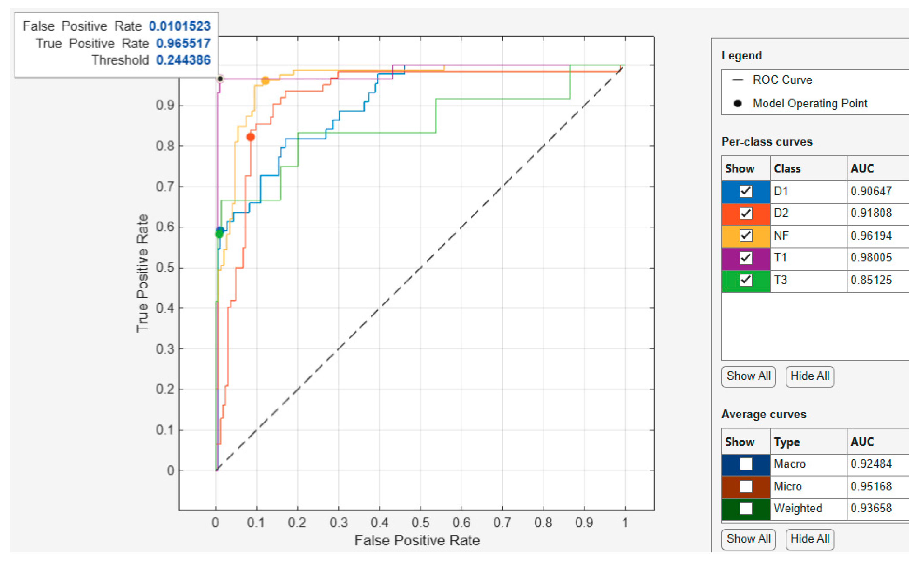
For the optimized Support Vector Machine model ROC-AUC curve shown in Figure 17, the model operating point with a threshold of 0.244386 used by the classifier to classify this observation shows the corresponding true positive rate of 0.965517 and false positive rate of 0.0101523. This indicates that a false positive rate of 0.01015 incorrectly classified 3.45% of the negative class observations to the positive class, and a true positive rate of 0.95 correctly classified 95% of the positive class. Regarding the AUC, the best performing class achieved an AUC value of 0.98005, which is close to the best value of 1. 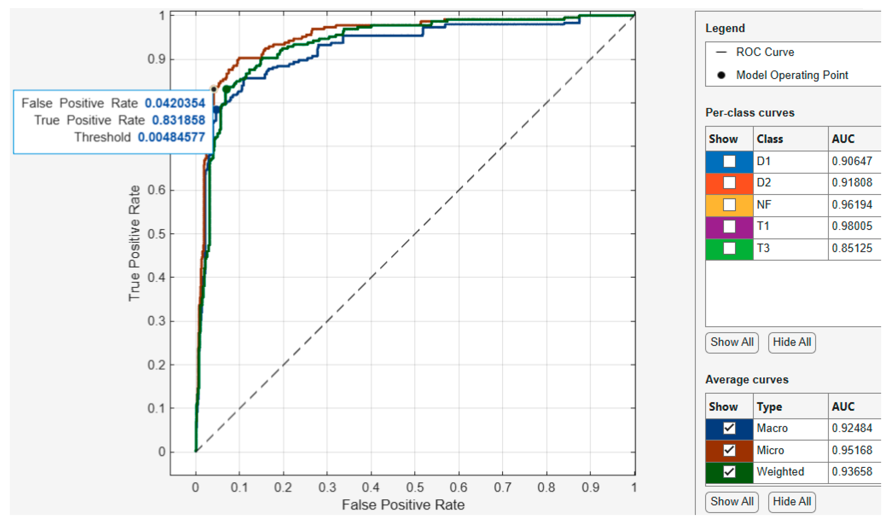Furthermore, when assessing the best performing average curve in Figure 18, the classifier used a threshold of 0.00484577 for the model operating point to classify observations with a corresponding true positive rate of 0.831858 and false positive rate of 0.0420354. This indicates that the false positive rate of 0.042 of the best performing average curve incorrectly classified 16.82% of the negative class observations as the positive class. Overall, the average curve has an AUC value of 0.95168, which is close to the best value of 1.

3.2.5. Optimized Decision Tree ROC-AUC Curve

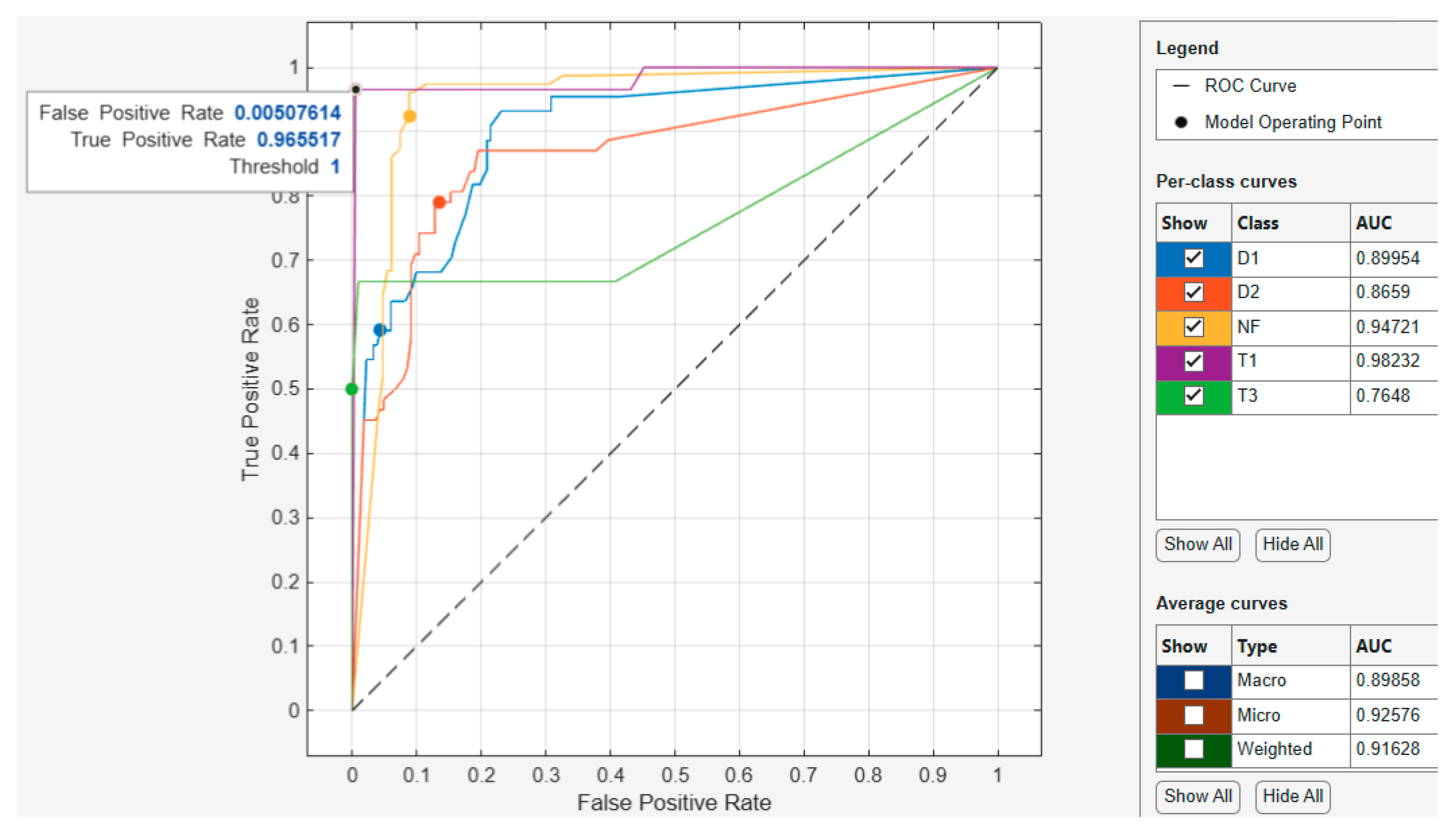
For the optimized Decision Tree model ROC-AUC curve shown in Figure 19, the model operating point with a threshold of 1 used by the classifier to classify this observation shows the corresponding true positive rate of 0.965517 and false positive rate of 0.00507614. This indicates that a false positive rate of 0.00507 incorrectly classified 3.45% of the negative class observations to the positive class, and a true positive rate of 0.95 correctly classified 95% of the positive class. Regarding the AUC, the best performing class achieved an AUC value of 0.98232, which is close to the best value of 1. Furthermore, when assessing the best performing average curve in Figure 20, the classifier used a threshold of 0.00 for the model operating point to classify observations with a corresponding true positive rate of 0.80531 and false positive rate of 0.0486726. This indicates that the false positive rate of 0.0486 of the best performing average curve incorrectly classified 19.47% of the negative class observations as the positive class. Overall, the average curve has an AUC value of 0.92576, which is close to the best value of 1.

A summary of the optimized machine learning results obtained in Section 3.2 is tabulated in

Table 3. Performance summary of the optimized classification algorithms.

Classifier	Accuracy % (Validation)	Accuracy % (Test)	Prediction Speed (obs/s)	Training Time (s)	Average Precision % (Validation)	Average Recall % (Validation)	Average F1-Score % (Validation)	Average Precision % (Test)	Average Recall % (Test)	Average F1-Score % (Test)
Ensemble	82.301	92.857	203.160	386.261	84.032	78.999	79.248	30.952	87.521	86.752
k-Nearest Neighbor	92.478	94.643	3691.54	15.926	91.802	91.380	91.540	95.446	92.206	93.036
Neural Networks	89.823	94.643	4369.429	372.426	89.607	89.534	89.518	31.548	89.317	88.374
Support Vector Machine	83.186	82.143	2051.096	1486.396	83.938	81.620	82.036	80.569	80.531	80.303
Decision Trees	80.531	89.286	7765.522	13.805	82.369	78.826	79.665	29.762	84.216	87.249

, which shows the overall performance of each optimized algorithm consisting of the key performance metrics considered for this study, i.e., accuracy, precision, recall, F1-score, and training time.

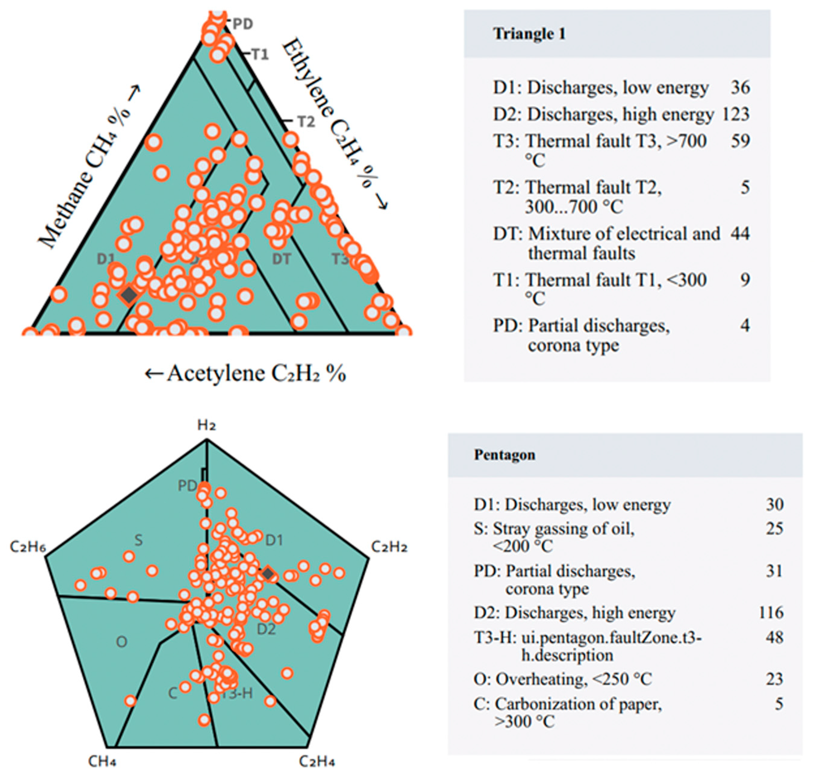
To assess the performance of the proposed optimized machine learning algorithms against the conventional methods, the two best performing methods as reported in various studies, i.e., the Duval Triangles and Pentagon, were subjected to the same DGA dataset of 282 samples used for the proposed optimized models using the Vaisala DGA Calculator software. From the computation of the methods, it was surprising to observe the misclassification rates of these methods, with both of them achieving relatively low classification accuracies of 35.76% and 30.82%, respectively.

This was hugely attributed to their inability to correctly classify non-fault samples with both failing to achieve notable classification on those samples, and this overshadowed their classification capabilities, which were observed on D1, D2, and T3 faulted samples. Figure 21 shows the graphical presentation and summary of the results obtained from the Vaisala DGA calculator software. These results are discussed in Section 4 where there is a tabulated comparison between the proposed optimized algorithms and the Duval Triangle and Pentagon methods.

4. Discussions

In this chapter, the performance of five optimized machine learning algorithms assessed in Section 3 using MATLAB Classification Learner is discussed. The results were presented using confusion matrices and various performance matrices, i.e., accuracy, precision, recall, F1-score, and ROC-AUC curves. These results (apart from ROC-AUC curves), were further tabulated to compare their performance, and the results are tabulated in

Table 4. Optimized machine learning models performance comparison against the conventional Duval Triangle and Pentagon methods.

Classification Method	D1	D2	NF	T1	T2	T3	PD	DT	S	O	C	Accuracy %
Actual Samples	55	77	100	36	0	14	0	0	0	0	0	-
Optimized Ensemble	36	66	98	35	0	3	0	0	0	0	0	82.30
Optimized kNN	48	71	98	35	0	10	0	0	0	0	0	92.48
Optimized Neural Network	47	71	93	35	0	9	0	0	0	0	0	89.82
Optimized SVM	34	62	95	35	0	8	0	0	0	0	0	83.19
Optimized Tree	35	63	93	35	0	6	0	0	0	0	0	80.53
Duval Triangle 1	36	123	2	9	5	59	4	44	0	0	0	35.76
Duval Pentagon	30	116	4	0	0	48	31	0	25	23	5	30.82

.

Table 4 shows how each classification method performed in comparison with the actual DGA dataset for each sample, and how the accumulated percentages are calculated. From these results, it is observed that the proposed optimized methods outperform the conventional methods of the Duval Triangle and Pentagon. The classification performance of the conventional methods was relatively low, where the Duval Triangle was capable of correctly classifying 35.76% of the dataset, followed by the Duval Pentagon, which only correctly classified 30.82% of the dataset. In contrast, out of the five studied optimized algorithms, the results show that the Optimized k-Nearest Neighbor, Optimized Neural Network, and Optimized Support Vector Machine are the best performing algorithms with performance accuracies of 92.478%, 89.823%, and 83.186%, respectively, compared to the 35.76% and 30.82% of the Duval Triangle and Duval Pentagon.

To assess their performance against the conventional methods, the same dataset used for the machine learning algorithms was used to evaluate the performance of the Duval Triangle and Duval Pentagon methods using Vaisala DGA software. The proposed models outperformed the conventional methods as they could only achieve classification accuracy of 35.757% and 30.818%, respectively. Despite the performance dominance that the optimized algorithms had over the conventional methods, they still exhibited some limitations. Based on the results analyzed in Table 4, the proposed optimized algorithms performed relatively well with high accuracies. However, some of these algorithms exhibited limitations and deficiencies in other evaluation matrices that would require trade-offs when selecting the preferred method. The optimized SVM computational training time was the longest amongst all the algorithms at 1486.4 s, despite its good performance in other metrics. For the Regularized Neural Network, the identified limitation lies in the unknown computational speed and time of the algorithm as these are also very important parameters in determining the overall performance and effectiveness of algorithms. Even though it was relatively fast in real time, the algorithm does not capture time. Apart from the performance of the models, another key factor that was encountered that was a limitation was access to the DGA datasets, which limited the number of samples that could be used for the study.

5. Conclusions

The purpose of this study was to investigate the application of machine learning algorithms for dissolved gas analysis-based fault classification to address the methodological gap presented by the conventional transformer fault classification methods in terms of their performance accuracy. From the proposed models, the best performing algorithm, Optimized k-Nearest Neighbor, achieved an overall performance accuracy of 92.478%, followed by the Optimized Neural Network at 89.823%. To assess their performance against the conventional methods, the same dataset used for the machine learning algorithms was used to evaluate the performance of the Duval Triangle and Duval Pentagon methods using Vaisala DGA software, the proposed models outperformed the conventional methods, as they could only achieve classification accuracy of 35.757% and 30.818%, respectively. Even though the proposed models performed fairly well, the misclassification of some of the transformer faults as indicated by the confusion matrices suggests further improvements. Future works could focus on the enhancement of the algorithm optimization and feature selection parameters.

References

- Saha, T.P.; Purkait, P. Transformer Ageing: Monitoring and Estimation Techniques, 1st ed.; John Wiley & Sons: Singapore, 2017; p. 9. [Google Scholar]
- Dladla, V.M.N.; Thango, B.A. Fault Classification in Power Transformers via Dissolved Gas Analysis and Machine Learning Algorithms: A Systematic Literature Review. Appl. Sci. 2025, 15, 2395. [Google Scholar] [CrossRef]
- Wajid, A.; Rehman, A.U.; Iqbal, S.; Pushkarna, M.; Hussain, S.M.; Kotb, H.; Alharbi, M.; Zaitsev, I. Comparative Performance Study of Dissolved Gas Analysis (DGA) Methods for Identification of Faults in Power Transformer. Int. J. Energy Res. 2023, 2023, 9960743. [Google Scholar] [CrossRef]
- Taha, I.B.; Ghoneim, S.S.; Zaini, H.G. Improvement of Rogers four ratios and IEC code methods for transformer fault diagnosis based on dissolved gas analysis. In Proceedings of the North American Power Symposium (NAPS), Charlotte, NC, USA, 4–6 October 2015; pp. 1–5. [Google Scholar]
- Sarma, G.S.; Reddy, R.; Nirgude, P.M.; Naidu, V. A review on real time fault detection and intelligent health monitoring techniques of transformer. Int. J. Eng. Res. Appl. 2021, 11, 40–47. [Google Scholar]
- Piotrowski, T.; Rozga, P.; Kozak, R.; Szymanski, Z. Using the analysis of the gases dissolved in oil in diagnosis of transformer bushings with paper-oil insulation—A case study. Energies 2020, 13, 6713. [Google Scholar] [CrossRef]
- Dladla, V.M.N.; Thango, B.A. Transformer Faults Multiclassification using Regularized Neural Network and Dissolved Gas Analysis. In Proceedings of the 2025 33rd Southern African Universities Power Engineering Conference (SAUPEC), Pretoria, South Africa, 29–30 January 2025; pp. 1–6. [Google Scholar] [CrossRef]
- IEEE. IEEE Guide for the Interpretation of Gases Generated in Mineral Oil-Immersed Transformers. In IEEE Std C57.104-2019 (Revision of IEEE Std C57.104-2008); IEEE: Piscataway, NJ, USA, 2019; pp. 1–98. [Google Scholar] [CrossRef]
- CIGRE. Guide on Transformer Intelligent Condition Monitoring (TICM) Systems; CIGRE: Paris, France, 2015; Volume 603. [Google Scholar]
- De Faria, H.; Costa, J.G.S.; Olivas, J.L.M. A review of monitoring methods for predictive maintenance of electric power transformers based on dissolved gas analysis. Renew. Sustain. Energy Rev. 2015, 46, 201–209. [Google Scholar] [CrossRef]
- Saad, M.; Tenyenhuis, E. On-line gas monitoring for increased transformer protection. In Proceedings of the IEEE Electrical Power and Energy Conference (EPEC), Saskatoon, SK, Canada, 22–25 October 2017. [Google Scholar]
- Alqudsi, A.Y.; ElHag, A.H. A cost effective artificial intelligence based transformer insulation health index. In Proceedings of the 3rd International Conference on Condition Assessment Techniques in Electrical Systems (CATCON), Punjab, India, 16–18 November 2017. [Google Scholar]
- Németh, B.; Vörös, C.; Csépes, G. Health index as one of the best practice for condition assessment of transformers and substation equipments—Hungarian experience. In Proceedings of the CIGRÉ Biennial Session A2-103, Paris, France, 24–29 August 2014. [Google Scholar]
- Sun, H.C.; Huang, Y.C.; Huang, C.M. A Review of Dissolved Gas Analysis in Power Transformers. Energy Procedia 2012, 14, 1220–1225. [Google Scholar] [CrossRef]
- Wani, S.A.; Rana, A.S.; Sohail, S.; Rahman, O.; Parveen, S.; Khan, S.A. Advances in DGA based condition monitoring of transformers: A review. Renew. Sustain. Energy Rev. 2021, 149, 111347. [Google Scholar] [CrossRef]
- CIGRE. New techniques for dissolved gas-in-oil analysis. Electra 2001, 198, 20–27. [Google Scholar]
- CIGRE. 771—Advances in DGA Interpretation. In Technical Brochure Joint Working Group A2/D1; CIGRE: Paris, France, 2019. [Google Scholar]
- Zhang, Y.; Li, X.; Zheng, H.; Yao, H.; Liu, J.; Zhang, C.; Peng, H.; Jiao, J. A Fault Diagnosis Model of Power Transformers Based on Dissolved Gas Analysis Features Selection and Improved Krill Herd Algorithm Optimized Support Vector Machine. IEEE Access 2019, 7, 102803–102811. [Google Scholar] [CrossRef]
- Jin, L.; Kim, D.; Chan, K.Y.; Abu-Siada, A. Deep Machine Learning-Based Asset Management Approach for Oil—Immersed Power Transformers Using Dissolved Gas Analysis. IEEE Access 2024, 12, 27794–27809. [Google Scholar] [CrossRef]
- Ghoneim, S.S.M.; Mahmoud, K.; Lehtonen, M.; Darwish, M.M.F. Enhancing Diagnostic Accuracy of Transformer Faults Using Teaching-Learning-Based Optimization. IEEE Access 2021, 9, 30817–30832. [Google Scholar] [CrossRef]
- Wang, L.; Littler, T.; Liu, X. Gaussian Process Multi-Class Classification for Transformer Fault Diagnosis Using Dissolved Gas Analysis. IEEE Trans. Dielectr. Electr. Insul. 2021, 28, 1703–1712. [Google Scholar] [CrossRef]
- Li, J.; Zhang, Q.; Wang, K.; Wang, J.; Zhou, T.; Zhang, Y. Optimal dissolved gas ratios selected by genetic algorithm for power transformer fault diagnosis based on support vector machine. IEEE Trans. Dielectr. Electr. Insul. 2016, 23, 1198–1206. [Google Scholar] [CrossRef]
- Aizpurua, J.I.; Catterson, V.M.; Stewart, B.G.; McArthur, S.D.J.; Lambert, B.; Ampofo, B.; Pereira, G.; Cross, J.G. Power transformer dissolved gas analysis through Bayesian networks and hypothesis testing. IEEE Trans. Dielectr. Electr. Insul. 2018, 25, 494–506. [Google Scholar] [CrossRef]
- Benmahamed, Y.; Teguar, M.; Boubakeur, A. Application of SVM and KNN to Duval Pentagon 1 for transformer oil diagnosis. IEEE Trans. Dielectr. Electr. Insul. 2017, 24, 3443–3451. [Google Scholar] [CrossRef]
- Prasojo, R.A.; Gumilang, H.; Suwarno; Maulidevi, N.U.; Soedjarno, B.A. A Fuzzy Logic Model for Power Transformer Faults’ Severity Determination Based on Gas Level, Gas Rate, and Dissolved Gas Analysis Interpretation. Energies 2020, 13, 1009. [Google Scholar] [CrossRef]
- Zhang, Y.; Wang, Y.; Fan, X.; Zhang, W.; Zhuo, R.; Hao, J.; Shi, Z. An Integrated Model for Transformer Fault Diagnosis to Improve Sample Classification near Decision Boundary of Support Vector Machine. Energies 2020, 13, 6678. [Google Scholar] [CrossRef]
- Ward, S.A.; El-Faraskoury, A.; Badawi, M.; Ibrahim, S.A.; Mahmoud, K.; Lehtonen, M.; Darwish, M.M.F. Towards Precise Interpretation of Oil Transformers via Novel Combined Techniques Based on DGA and Partial Discharge Sensors. Sensors 2021, 21, 2223. [Google Scholar] [CrossRef] [PubMed]
- Available online: https://www.mathworks.com/help/stats/fitctree.html (accessed on 1 March 2025).
- Available online: https://www.mathworks.com/discovery/support-vector-machine.html?s_tid=srchtitle_support_results_1_Understanding+Support+Vector+Machine (accessed on 1 March 2025).
- Available online: https://www.mathworks.com/help/stats/referencelist.html?type=function&s_tid=CRUX_topnav&category=classification-ensembles (accessed on 1 March 2025).
- Available online: https://www.mathworks.com/help/stats/fitcnet.html (accessed on 1 March 2025).
- Available online: https://www.mathworks.com/help/stats/fitcknn.html (accessed on 1 March 2025).
- Available online: https://www.mathworks.com/help/stats/fitcensemble.html (accessed on 1 March 2025).
- Markoulidakis, I.; Rallis, I.; Georgoulas, I.; Kopsiaftis, G.; Doulamis, A.; Doulamis, N. Multiclass Confusion Matrix Reduction Method and Its Application on Net Promoter Score Classification Problem. Technologies 2021, 9, 81. [Google Scholar] [CrossRef]
- Available online: https://www.mathworks.com/help/stats/assess-classifier-performance.html#mw_7eb6ae10-bff9-47fb-b16a-007141f95641 (accessed on 19 April 2025).
- Tourassi, G. Receiver Operating Characteristic Analysis: Basic Concepts and Practical Applications. In The Handbook of Medical Image Perception and Techniques; Samei, E., Krupinski, E.A., Eds.; Cambridge University Press: Cambridge, UK, 2018; pp. 227–244. [Google Scholar]
- Available online: https://www.blog.trainindata.com/auc-roc-analysis/ (accessed on 19 April 2025).
Figure 1.
Machine learning algorithms families used in this study.
Figure 2.
Proposed multiclassification model flowchart.
Figure 3.
A multiclassification confusion matrix principle.
Figure 4.
Typical ROC-AUC curves and their performance measurement matrix adapted from [
37].
Figure 5.
VAISALA DGA calculator software interface.
Figure 6.
Optimized Ensemble algorithm confusion matrix.
Figure 7.
Optimized k-Nearest Neighbor algorithm confusion matrix.
Figure 8.
Optimized Neural Network algorithm confusion matrix.
Figure 9.
Optimized Support Vector Machine algorithm confusion matrix.
Figure 10.
Optimized Tree algorithm confusion matrix.
Figure 11.
Optimized Ensemble validation ROC curve (per class).
Figure 12.
Optimized Ensemble validation ROC curve (average curves).
Figure 13.
Optimized k-Nearest Neighbor validation ROC curve (per class).
Figure 14.
Optimized k-Nearest Neighbor validation ROC curve (average curves).
Figure 15.
Optimized Neural Network validation ROC curve (per class).
Figure 16.
Optimized Neural Network validation ROC curve (average curves).
Figure 17.
Optimized Support Vector Machine validation ROC curve (per class).
Figure 18.
Optimized Support Vector Machine validation ROC curve (average curves).
Figure 19.
Optimized Decision Tree validation ROC curve (per class).
Figure 20.
Optimized Decision Tree validation ROC curve (average curves).
Figure 21.
Duval Triangle and Pentagon results.